Introduction
Today, on many farms, automatically recording reliable milk yields from each milking is well-established. Furthermore, in diverse test stations or dairy research farms, water intake and feed intake are measured automatically and completely (e.g. Coffey et al., Reference Coffey, Simm and Brotherstone2002; Hüttmann, 2007; Kramer et al., Reference Kramer, Stamer, Mahlkow, Lüpping and Krieter2008). In the future, it is imaginable that cost-efficient and reliable sensor technology will automatically measure traits such as somatic cell score or fat and protein content of milk on practical dairy farms (Ordolff, Reference Ordolff2005; Svennersten-Sjaunja et al., Reference Svennersten-Sjaunja, Sjögren, Andersson and Sjaunja2005; DeLaval, 2008). For such datasets with repeated daily measures within cow, it is assumed that the repeated measures are not independent and thus autocorrelated (Littell et al., Reference Littell, Henry and Ammerman1998; Littell et al., Reference Littell, Milliken, Stroup, Wolfinger and Schabenberger2006). Thus, for valid statistical inference and correct variance components, it is necessary to achieve the best model fit by using applicable error covariance structures (Bonham and Reich, Reference Bonham and Reich1999; Sawalha et al., Reference Sawalha, Keown, Kachman and van Vleck2005a; König et al., Reference König, Köhn, Kuwan, Simianer and Gauly2006; Rosário et al., Reference Rosário, Silva, Coelho and Savino2007). Taking different covariance structures for the residuals of repeated measures into account, Bonham and Reich (Reference Bonham and Reich1999) estimated different variance components and found varying significances of least square means. Generally, it is assumed for repeated measures that measurements closer together have higher correlations than measurements with a longer time gap between them (Littell et al., Reference Littell, Milliken, Stroup, Wolfinger and Schabenberger2006). In the literature, there are only few results concerning existing autocorrelations and correlation patterns of daily milk yield, feed intake and water intake. Stamer (1995) found moderate autocorrelations between adjacent measures of daily yields of dry matter intake with p 1 = 0.02, but for measurements two units apart, the author found a correlation of p 2 = 0.10. Hüttmann (2007) assessed the autocorrelation between adjacent milk yield measures on p 1 = 0.30 and for p 2 a correlation of 0.26 was found. According to this, it is assumed that random regression models, estimating covariance functions for the additive genetic and permanent environmental effect, but not accounting for a relationship between errors, are not yet adequate to analyse daily yields, and thus covariance structures for the residuals have to be applied (Littell et al., Reference Littell, Milliken, Stroup, Wolfinger and Schabenberger2006; Mielenz et al., Reference Mielenz, Spilke, Krejcova and Schüler2006). For this purpose, fixed regression (FR) and random regression (RR) models with several candidate covariance structures were compared using different model fit statistics to select an appropriate covariance model. Fortunately, access to daily measurements of a dairy research farm enabled us to look at the suitability of such models. Thus, the daily measured traits milk yield, water intake and dry matter intake were analysed to find possible error covariance patterns. Finally, significance results for an included fixed effect are illustrated for different model variants in order to show the consequences of considering a proper covariance structure.
Material and methods
Data
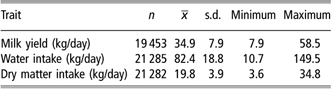
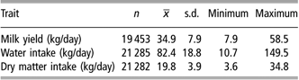
Data were recorded on the Futterkamp dairy research farm of the Chamber of Agriculture of Schleswig-Holstein. The period of recording was between March 2005 and April 2006. The dairy herd was subdivided into a research and a production herd. During data collection, three feeding experiments were performed with the research herd. This herd with a frequently changing cow stock comprising nearly 70 cows, divided into two feeding groups (Group A and Group B). Observations from about 21 000 cow-days were accumulated from 178 Holstein cows during the feeding experiments. Between the feeding experiments, dry matter intake was not recorded. Cows were milked twice daily and they were fed an ad libitum total mixed ration also twice daily. The feeding and the water troughs developed and installed by the company INSENTEC were equipped with an individual cow identification system; hence the cows were able to pass the troughs only one at a time. Each visit to the water and feeding trough was routinely recorded and the amounts of collected feed and water were accumulated to daily yields. Furthermore, each milking for the trait milk yield was recorded with the milk meters technology of the company DeLaval. Extreme values (mainly for the traits water intake and dry matter intake) that deviated more than ±4 s.d. were excluded from the dataset. Thus, for the traits milk yield, water intake and dry matter intake, observed values 7.9 to 58.5, 10.7 to 149.5 and 3.6 to 34.8 kg, respectively, were taken into account (Table 1), while the average amount of dry matter was about 45% during the data collecting period. In addition, 25 cows with less than 40 daily observations per trait and also two cows with records in only one of the three traits were excluded from the dataset. Furthermore, 6 complete days could not be considered because of the exclusion of the first and the last day of each feeding experiment and 3 days due to general technical problems during the data collecting period. A total of about 3500 records were excluded from further investigations. The lower number of records for the trait milk yield – in contrast to the traits water intake and dry matter intake – is due to gaps in the dataset, which resulted particularly from antibiotic treatments of the cows and their subsequent withdrawal periods.
Means ( ), standard deviations (s.d.) and range (minimum, maximum) of the three analysed traits
The cows belonged to parities 1 to 9 and the lactation days were between 6 and 230. The number of cows with observations from two lactations was 24.
Data analysis
Modelling of the expected value structure
Preliminary investigations were performed using the SAS (2005) software in order to identify relevant fixed effects. Two different models – FR and RR – were used. Both model variants contained the fixed effect of the lactation curve, which was calculated by average regression coefficients universally valid for all cows. Due to the fact that the coefficients are constant and fixed for all animals, the corresponding models are called FR models. In contrast, the RR models include additional regression coefficients. These are computed for every animal, which is usually considered as a random effect in the mixed model (van der Werf, 2001). These coefficients are therefore indicated as RR coefficients and the corresponding models as RR models. Thus, RR models allow the estimation of cow-specific lactation curves (Schaeffer and Dekkers, 1994; Schaeffer, Reference Schaeffer2004). RR models are increasingly used for the estimation of breeding values and commonly recommended for statistical analysis in this area (e.g. Koenen and Veerkamp, Reference Koenen and Veerkamp1998; Veerkamp and Thompson, Reference Veerkamp and Thompson1999). In addition, FR models were used to allow comparison of our results to those reported by others, which are mainly based on FR models. Both alternatives (FR, RR) contained the fixed effects parity, group test day and (as described) a function of the day of lactation and the random effects cow and error term. The group test day was included as a common test day within feeding group effect in order to consider the possible influences of the different feeding rations. Parities were divided into three classes: first lactation, second lactation, and third and higher lactations.
Model I (FR):

where yijkl are the observations of milk yield, dry matter intake or water intake, μ is the overall mean, LNRi is the fixed effect of the ith parity class (i = 1,.., 3), GTDj is the fixed effect of the jth test day within the feeding group (j = 1,…, 658), bim are the FR coefficients within the ith lactation with, xijkl 1(DIM) = (DIM/305), xijkl 2(DIM) = (DIM/305)2, xijkl 3(DIM) = ln(305/DIM) and xijkl 4(DIM) = (ln(305/DIM))2, where DIM is the days in milk, ck is the random effect of the kth cow (k = 1,.., 178), eijkl is the random error.
Model II (RR) was used to model cow-specific lactation curves by applying the function according to Ali and Schaeffer (Reference Ali and Schaeffer1987).
Model II (RR):

where ckm are the RR coefficients within the kth cow (k = 1,…, 178), with xijkl 0(DIM) = 1, xijkl 1(DIM) = (DIM/305), xijkl 2(DIM) = (DIM/305)2, xijkl 3(DIM) = ln(305/DIM) and xijkl 4(DIM) = (ln(305/DIM))2.
Within the analysis of dry matter intake, the numerical optimisation of the restricted likelihood did not converge. Instead, the following polynomial term of the second degree was used:  .
Modelling the lactation curves for the trait milk yield has been a frequently discussed topic in the literature (e.g. Wood, Reference Wood1967; Grossman and Koops, Reference Grossman and Koops1988; Kirkpatrick et al., Reference Kirkpatrick, Hill and Thompson1994; Jamrozik and Schaeffer, Reference Jamrozik and Schaeffer1997; van der Werf, 2001; Sylvestre et al., Reference Sylvestre, Petim-Batista and Colaco2006). López-Romero and Carabaño (Reference López-Romero and Carabaño2003) noted that functions frequently used for the modelling of lactation curves are those proposed by Ali and Schaeffer (Reference Ali and Schaeffer1987) or Wilmink (Reference Wilmink1987). In addition, also quite often used are Legrende polynomials (e.g. Liu et al. (Reference Liu, Zhang, Schaeffer, Yang and Zhang2006) for milk yield and Coffey et al. (Reference Coffey, Simm and Brotherstone2002) for the traits feed intake and energy balance). Sylvestre et al. (Reference Sylvestre, Petim-Batista and Colaco2006) hyphothesised that this function is able to fit daily data superior than functions with less than five parameters such as Wilmink (Reference Wilmink1987), Wood (Reference Wood1967) or Legrende polynomials of less than four degrees. Also for modelling of feed intake and energy balance amongst others, Woodford et al. (Reference Woodford, Murphy and Davis1984), de Vries et al. (Reference de Vries, van der Beek, Kaal-Lansbergen, Ouweltjes and Wilmink1999) and Collard et al. (Reference Collard, Boettcher, Dekkers, Petitclerc and Schaeffer2000) used the Ali and Schaeffer function. Therefore, the function according to Ali and Schaeffer (Reference Ali and Schaeffer1987) was chosen for the analysis of all three traits.
The significance of fixed effects was tested by the F-test implemented in the MIXED procedure in SAS (2005). With regard to preconditions for linear models, homogeneity of variance was checked by plots of the standardised residuals against the predicted values. Additionally, these plots provided information about potential outliers. Furthermore, the frequency plots of the residuals were checked by visual inspection and confirmed the assumption of their normal distribution.
Modelling error covariance structures
Dependencies between the residuals of repeated yields of a cow can be modelled with covariance structures (Sawalha et al., Reference Sawalha, Keown, Kachman and van Vleck2005a and Reference Sawalha, Keown, Kachman and van Vleck2005b; Mielenz et al., Reference Mielenz, Spilke, Krejcova and Schüler2006). In order to obtain basic knowledge about actual covariances between all residuals, the complete parameterised covariance structure UNSTRUCTURED should be estimated. It might then be possible to recognise underlying patterns. But this type of matrix is too complex, since all variances and covariances are different and too large matrices would then have to be calculated. According to Jennrich and Schluchter (Reference Jennrich and Schluchter1986), the number of estimatable parameters is q = (T*(T + 1))/2, where T is the length of the time series. With a maximum length of time series in our dataset of about 225 measures (lactation day 6 to 230), the number of parameters to estimate would arise to q = 25 425. Of course this requires too much computational effort and is not applicable to our computing capacity. As a compromise, three minor complex alternatives of covariance structures were tested: the first-order autoregressive model (AR(1)), the spatial (exponential) structure (SP(EXP)) and the TOEPLITZ(4) model (TOEP(4)), which assume constant residual variance at the different stages of lactation. Estimation of heterogenous residual variances within these patterns was not possible due to no positive definite Hessian matrices. To check the assumption of error variance homogeneity, the residual variances were estimated separately within three lactation stages (days in milk 30 to 70, 110 to 150 and 190 to 230) using the FR + TOEP(4) model.
It should be indicated that the notation only gives the upper triangular part of the matrices.
(i) First-order autoregressive model (AR(1))

Under the AR(1) model, the correlation between adjacent within-subject errors is p, regardless of whether the pair of observations is the 1st and 2nd, 2nd and 3rd, or (d−1)th and dth (Littell et al., Reference Littell, Milliken, Stroup, Wolfinger and Schabenberger2006). For any pair of errors that are two units apart the correlation is p 2, and, in general, errors d units apart have correlation p d.
(ii) Spatial (exponential) structure (SP(EXP))
For the SP(EXP) structure, the correlations decline as a function of time. The function is defined as g exp (d) = e(−(d/p)), where d is the temporal distance between two measurements at times t 1 and t 2, d = |t 1−t 2|. The SP (EXP) structure models the covariance between t 1 and t 2 as Cov [Yt 1, Yt 2] = σe 2*e(−(d/p)). The SP(EXP) type can be used for unequally spaced data with characteristic different distances between the measures. It is only a generalisation of the AR(1) type for unequally spaced data and it is expected to deliver the same information criteria as AR(1) when the data are equally spaced (Littell et al., Reference Littell, Milliken, Stroup, Wolfinger and Schabenberger2006).
(iii) TOEPLITZ model TOEP(4)

For TOEP(4), the number 4 is the number of the estimated parameters  plus three covariance parameters. The TOEP(4) model is similar to the AR(1) model, because pairs of within-subject errors separated by a common lag have the same correlation. However, errors d units apart have correlation pd instead of p d (Littell et al., Reference Littell, Milliken, Stroup, Wolfinger and Schabenberger2006).
In order to avoid biased results with the application of AR(1) and TOEP(4), complete time series with equal distances between the observations (~equally spaced data) are recommended (SAS, 2005). Therefore, missing values (10% of the records for milk yield and 4% of the records for water intake and dry matter intake) were replaced by the mean value of the prior 3-day period. It should be emphasised that replacing missing values is problematic and possibly biases the results. Otherwise, the corresponding error was assumed to be moderate due to the marginal number of replaced missing values. Nevertheless, comparing different error covariance structures for the new traits water intake and dry matter intake require the replacing of missing values.
Criteria for the selection of models
Model selection was based on the restricted maximum-likelihood principle (REML). The procedure MIXED in SAS (2005) provides by default different model selection criteria (Mielenz et al., Reference Mielenz, Spilke, Krejcova and Schüler2006). Models, of which the former one could be reduced to a special case of the latter one, were compared by applying the likelihood ratio test (LRT), which is a statistical test of the quality of the fit of two hierarchically nested models. Those models are identical in their design matrices of the fixed model parameters. The LRT is calculated as the difference Δ(−2 log L) of the two comparable models and approximates a χ 2 distribution with Δq degrees of freedom, where q is the number of estimated covariance components of each model.
Models with different covariance structures for the repeated measures are not hierarchically nested. For the comparison of these models, the information criteria of Akaike (1973) (AIC, Akaike’s information criteria) and Schwarz (Reference Schwarz1978) (BIC, Bayesian’s information criteria) were used. These values take the number of estimated parameters into account and prefer less-complex model variants. For the decision, the model with the smallest values for AIC and BIC has to be selected without making a statement about the underlying significance. In contrast, the LRT yields a significance test under the null hypothesis that the reduced model is correct. Thus, both information criteria on the one hand and the LRT on the other hand can lead to different results during the model selection process (Pitt et al., Reference Pitt, Myung and Zhang2002).
In addition, the investigation of the impact of model choice on drawing inference from the data analysis was enclosed. Thus, the model with the best ability to fit was compared with a less-complex model by significance results for one fixed effect.
Results
Preconditions for linear mixed models
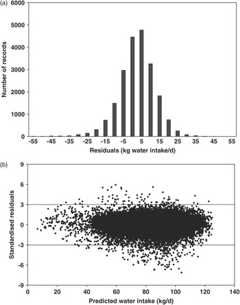
For all three traits, the frequency plot of the residuals was visualised in order to detect deviations from a normal distribution. Additionally, homogeneity of variance of the residuals was judged by visual inspection of the plots of the standardised residuals against the predicted values. As an example, the frequency plot of the residuals (Figure 1a) and the plot of the standardised residuals against the predicted values (Figure 1b) obtained from Model I (FR) are given for the trait water intake. It was concluded that the residuals were normally distributed and that their variance was homogenous over the whole range of the predicted estimates. Most residuals were in the range of ±3 s.d. A total of 0.92% of all residuals were smaller than −3 s.d. and 0.26% of all residuals were greater than +3 s.d. Also for milk yield and dry matter intake, normal distribution and variance homogeneity arose from the adequate plots (not presented).
Frequency plot (a) of the residuals and plots of the standardised residuals against the predicted water intake (b) after fitting the data with Model I.

Lactation curves
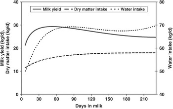
In order to provide evidence about the modelling quality of the underlying function according to Ali and Schaeffer (Reference Ali and Schaeffer1987), the lactation curves are shown in Figure 2. The curves were hardly affected by the applied model and the presented ones are obtained from Model I (FR) for primiparous cows and for the three traits.
Lactation curves for milk yield, dry matter intake and water intake for primiparous cows after fitting with Model I.

For milk yield, the characteristic course of the curve with an increase at the beginning up to 50 days and a subsequent slight decline was as expected. The trajectory for water intake was similar, but at a higher level. In contrast to the trait milk yield, it took longer to achieve the maximum level, and it also declined slightly in further lactation. In contrast, the trait dry matter intake increased along the whole lactation.
Comparison of FR and RR models with different error covariance structures
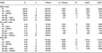
For the three traits, the residual variance, the restricted log likelihood values and information criteria of the different models are given in Table 2. The results for the alternatives AR(1) and SP(EXP) were exactly the same because of the application of equally spaced data as shown by Littell et al. (Reference Littell, Milliken, Stroup, Wolfinger and Schabenberger2006). Thus, the covariance structure SP(EXP) is not listed in Table 2. Within a trait, all model variants except the FR + AR(1) model were hierarchically nested. The differences between these nested models were all classified as highly significant (P < 0.01) using the LRT. The results of the LRT and the information criteria AIC and BIC did not lead to different conclusions for model selection.
Estimated residual variance, restricted log likelihood and information criteria of the different models for all three traits

AIC = Akaike’s information criteria; BIC = Bayesian’s information criteria; FR = fixed regression; RR (AS) = random regression with the function of Ali and Schaeffer (Reference Ali and Schaeffer1987); RR (p 2) = random regression with polynomial of second degree;  = residual variance; q = number of covariance components, d.f. = degrees of freedom.
For all traits, the classic FR model had the highest restricted log likelihood and the highest AIC and BIC values (where smaller is better), so that fitting was better for every alternatively tested model. In addition, modelling the cow-specific lactation curve with the RR model indicated much lower restricted log likelihood, AIC and BIC values for all traits.
Furthermore, including different covariance structures to model the dependencies between repeated measures showed similar tendencies for water intake and dry matter intake in contrast to milk yield. For water intake and dry matter intake, the FR + AR(1) model provided only a moderately but significantly better fitting. In contrast to the FR + AR(1) model, the FR + TOEP(4) model provided much better information criteria for the traits water intake and dry matter intake. For milk yield, the FR + AR(1) and the FR + TOEP(4) models delivered much better model fitting in contrast to the FR variant, but the AIC and BIC values were nearly the same for these two variants.
The differences of quality of fit between the AR(1) and the TOEP(4) covariance structures were also found along with the RR models for the traits water intake and dry matter intake and even for milk yield. Comparing all model variants, the best fit was achieved with the most complex RR + TOEP(4) model.
Homogeneity of residual variance and correlations between residual effects
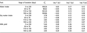
The residual variances and the correlations between the repeated measures within the different lactation stages are presented in Table 3. Hence, the assumption of homogenous residual variances can be checked. Due to the best fit, the RR + TOEP(4) model should have been chosen, but in order to avoid convergence problems with RR models due to the small number of included observations, the FR + TOEP(4) model was used instead.
Estimated residual variance and correlations for the different lags at different stages of lactation after modelling with the FR + TOEP(4) model

 = residual variance.
For water intake and dry matter intake, residual variance varied only marginally between the beginning, the middle and the end of the lactation in contrast to the estimates for the whole lactation. For milk yield, different estimates were found for the whole lactation ( = 5.44) in contrast to the separate lactation stages (
 = 4.00, 3.65 and 3.05, respectively). The correlations between the adjacent repeated measures of water intake, dry matter intake and milk yield, estimated for the whole lactation, were p 1 = 0.03, −0.05 and 0.48, respectively. For measurements two units apart, the correlations were p 2 = 0.17, 0.12 and 0.36, respectively, while they were assessed on p 3 = 0.12, 0.10 and 0.21, respectively, for water intake, dry matter intake and milk yield measurements with a lag of three observations. The correlations estimated for the different stages of lactation differed only marginally in contrast to those estimated for the whole lactation, with the exception of p 1 and p 2 for milk yield. For the whole lactation, the correlation p 1 was 0.48 in comparison to p 1 = 0.33, 0.35 and 0.29 for the three different lactation stages.
Model choice and statistical inference
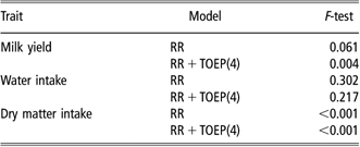
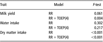
The influence of the model choice on the results of significance tests was proven by comparing the model with the best fit (RR + TOEP(4)) with the RR model without error covariance structures. In the case of the fixed effect parity, the inclusion of the error covariance structure TOEP(4) showed a clear influence on the accuracy of the inference (Table 4). For milk yield, the significance value of the global F-test levels altered with the consequence of another conclusion. Parity was not statistically significant (P = 0.061) in the RR model, it was significant (P = 0.004) in the other model.
Significance values (P) for the fixed effect parity and for the differences between least square means of parity levels dependent on trait and model
RR = random regression.
Discussion
Lactation curves
The lactation curve for milk yield showed the characteristic course, which had been shown frequently before (amongst others Veerkamp and Thompson, Reference Veerkamp and Thompson1999; Hüttmann, 2007). The lactation curve for water intake showed a path similar to the curve for milk yield with only a shift in level, which was also observed by Murphy et al. (Reference Murphy, Davis and McCoy1983). Similar lactation curves for dry matter intake were also found by Veerkamp and Thompson (Reference Veerkamp and Thompson1999) and Hüttmann (2007). The given course was similarly expected after inspecting the trajectory of the raw data. This is indeed not an evidence but an indication that the parameters according to Ali and Schaeffer (Reference Ali and Schaeffer1987) are also suitable to model the lactation curves of the traits water intake and dry matter intake.
Comparison of FR and RR models with different error covariance structures
For all traits, the RR models had much lower information criteria in contrast to the classic FR models. Similar results were found by Hüttmann (2007) for daily milk yield and dry matter intake with different FR and RR models. With RR models, water intake, dry matter intake and milk yield dynamics are modelled separately for every lactation day, which leads to a more effective consideration of the underlying biology and therefore to much more precise results (van der Werf, 2001; Mielenz et al., Reference Mielenz, Spilke, Krejcova and Schüler2006).
Inclusion of different error covariance structures along either FR or RR models again improved the values of the information criteria and thus the model fit for all three traits. But it seems that different covariance patterns are indicated for the three traits.
In detail for milk yield, model fit under the FR models was similar when comparing the AR(1) with the TOEP(4) pattern. The assumption of Littell et al. (Reference Littell, Milliken, Stroup, Wolfinger and Schabenberger2006) that adjacent daily measures are higher correlated than measures with lags of more units apart could be confirmed with both covariance structures. High dependencies between the repeated measures were found (p 1 = 0.65, p 2 = (0.65)2 = 0.42, p 3 = (0.65)3 = 0.27 with the FR + AR(1) model and p 1 = 0.48, p 2 = 0.36, p 3 = 0.21 with the FR + TOEP(4) model, respectively). The estimated correlations were similar and thus the differences between the patterns of the covariance structures had no effect. Along with the RR models, clear differences between AR(1) and TOEP(4) were found. With the inspection of the corresponding correlations estimated for these model variants (p 1 = 0.40, p 2 = (0.40)2 = 0.16, p 3 = (0.40)3 = 0.03 with the RR + AR(1) model and p 1 = 0.32, p 2 = 0.27, p 3 = 0.17 with the RR + TOEP(4) model), it is obvious that with the RR + AR(1) model the exponential decline in the correlations is too fast. In contrast, the correlations assessed with the RR + TOEP(4) model seem to be more realistic. Similar correlations (p 1 = 0.30, p 2 = 0.23, p 3 = 0.13) with an RR + TOEP(4) model for repeated milk intakes were found by Hüttmann (2007).
For dry matter intake and water intake, model fit was much better with the TOEP(4) model in contrast to the AR(1) model regardless of whether the FR or RR model was applied. The covariance structure AR(1) acts on the assumption that adjacent measures are higher correlated than those with more units between them (Littell et al., Reference Littell, Henry and Ammerman1998; Littell et al., Reference Littell, Milliken, Stroup, Wolfinger and Schabenberger2006). This seems to be the main reason as to why the AR(1) structure misrepresents the dependencies and patterns of the repeated measures of water intake and dry matter intake. Under the FR model, the AR(1) matrix valued the correlation for adjacent measures of dry matter intake and water intake at p 1 = 0.08 and 0.05. The corresponding correlations p 2 and p 3 were hence (0.08)2 = 0.0064 and (0.08)3 = 0.000512 for dry matter intake and (0.05)2 = 0.0025 and (0.05)3 = 0.000125 for water intake, which is almost equal to zero. With the TOEP(4) model, the correlations were p 1 = −0.05, p 2 = 0.12 and p 3 = 0.10 for dry matter intake and p 1 = 0.03, p 2 = 0.17 and p 3 = 0.12 for water intake (see also Table 3). Thus it appears to be the case that measures with a lag of two units apart are the highest correlated and even for measures three units apart correlations do exist. The correlations for repeated dry matter intakes are in agreement with the investigations of Stamer (1995), who found under an FR + TOEP(3) model an autocorrelation between adjacent measures of p 1 = 0.02 and between measures two units apart of p 2 = 0.10, while the AR(1) model showed no autocorrelation between repeated measures. In addition, the AIC value was lowest for the variant with a TOEP(3) covariance structure. Hüttmann (2007) found under an RR + TOEP(4) model a similar correlation pattern with p 1 = 0.07, p 2 = 0.10 and p 3 = 0.07 for repeated measures of dry matter intake, too. This model variant also provided by far the best fitting ability in contrast to models with an underlying AR(1) covariance structure. Thus, under a TOEPLITZ matrix the correlation pattern between repeated measures of dry matter intake and also water intake is assumed to be estimated more precisely. Maybe the physiology of these two coherent traits (correlation between cow effects is rc = 0.73 according to Kramer et al., Reference Kramer, Stamer, Mahlkow, Lüpping and Krieter2008) underlies another more enduring biorhythm than from day to day and therefore adjacent repeated measures are not necessarily the highest correlated. Of course this is speculative.
Generally, according to the fitting ability, the most complex RR + TOEP(4) model has to be emphasised for the analysis of daily yields of milk intake, water intake and dry matter intake. This is in accordance with the investigations of Hüttmann (2007), who obtained the best goodness of fit with a TOEP(4) model for the traits milk yield, feed intake, energy balance and body weight.
Homogeneity of residual variance and correlations between residual effects
The residual variance of water intake and dry matter intake varied only marginally between the beginning, the middle and the end of the lactation in contrast to the estimates for the whole lactation. For milk yield, residual variance estimated for the whole lactation was different from those estimated for the separate lactation sections. Residual variance seems to vary in the course of lactation. Jamrozik and Schaeffer (Reference Jamrozik and Schaeffer1997) clearly found higher residual variances for milk yield in the first lactation days in contrast to further lactation. This seems to be similar in the present study and can explain the higher residual variance estimated for the whole lactation ( = 5.44) in contrast to the separate sections of lactation (
 = 4.00, 3.65 and 3.05, respectively), because the first lactation days are not included in the first section (days in milk 30 to 70), but they are included for the whole lactation (days in milk 5 to 230). Furthermore, the correlations p 1, p 2 and p 3 estimated for the whole lactation differed only marginally from those correlations estimated for the separate lactation sections, exceptionally p 1 and p 2 for milk yield. Maybe this is also due to the inclusion of the first lactation days in the whole lactation, which seem to be somewhat different in contrast to further lactation.
For water intake and dry matter intake, the almost constant residual variances and correlations in the lactation trajectory gave evidence that assuming constant residual variances with the different covariance structures was reasonable. Thus, the emphasis for the use of the RR + TOEP(4) for daily yield data of these traits can be made without having made incorrect assumptions. For milk yield, error covariance structures with supposed heterogenic residual variances would have delivered a more correct fit but are difficult to compute.
Model choice and statistical inference
The choice of the right model is very important for drawing the correct inference from the analysed data (van der Werf, 2001). Thus, the model with the best fit RR + TOEP(4) was compared with the RR model. For the fixed effect parity, the inclusion of the error covariance structure TOEP(4) showed a clear influence on the accuracy of the inference. Parity was not statistically significant (P = 0.061) in the RR model, while it was significant (P = 0.004) in the other model. Varying significance values among the applied model variants is very important for the interpretation of statistical analyses. Imagine feeding research where the effect of a feeding additive on milk yield is tested and the effect would be significant under the applied model while it would be no longer significant under the more correct model. The consequences of such biased results could cause large economic losses for dairy farms. Inclusion of error covariance structures influences also the variance components of test day milk, fat and protein yields and test day somatic cell scores (Sawalha et al., Reference Sawalha, Keown, Kachman and van Vleck2005a) and also of daily voluntary milking frequency in an automatic milking system (König et al., Reference König, Köhn, Kuwan, Simianer and Gauly2006). The authors postulated the use of autoregressive error covariance structures for such data in order to prevent bias in heritabilities, because models without error covariance structures seem to overestimate the heritabilities. Similar conclusions in another research area were indicated by Bonham and Reich (Reference Bonham and Reich1999). These authors showed for autocorrelated data that inclusion of spatial autoregressive error covariance structure delivered the best linear unbiased estimates of parameters and also reduced the significance of differences between treatments of oil spills. Hence, in order to obtain certain preferable results, it is always necessary to aspire to use the model with the best fit.
Practical implementation
To obtain correct statistical inference, the results emphasise the use of adequate error covariance structures with RR models for the analysis of daily yields such as milk yield, water intake and dry matter intake, respectively. With equally spaced datasets, the use of the TOEP(4) error covariance structure must be postulated. Under practical conditions, daily data (e.g. milk yield) provide probably cow time series with gaps due to technical bugs or diseases of cows. In this regard, Mielenz et al. (Reference Mielenz, Spilke, Krejcova and Schüler2006) did not fill up the lacks of daily feed intake data. With such datasets they emphasised the use of an RR + SP(EXP) model. This type of covariance structure could be a compromise for practical implementation, because for all traits including this would be better than a complete omission of error covariance structures. Generally, it would be necessary for the future to investigate daily yield data of other traits with regard to the possible autocorrelation patterns.
Conclusion
The comparison of the conventional FR model and RR models with or without covariance structures for the repeated measures showed best model fitting with the most complex RR + TOEP(4) model for all traits. Autocorrelations between daily yields could be found and the covariance structure TOEP(4) was most suitable to indicate the dependencies of the repeated measures. The model choice influenced the significance values of the fixed effect parity and therefore the general inference of the data analysis. Thus, despite its complexity the RR + TOEP(4) model is recommended for use for analysis of equally spaced datasets of milk yield, water intake and dry matter intake.