2. Data

2.1 The data used in this paper are the all-cause number of deaths aged x last birthday during each calendar year y, split by gender. Corresponding mid-year population estimates are also given. The data therefore lend themselves to modelling the force of mortality, $$${{\mu }_{x\: + \:\frac{{\rm{1}}}{{\rm{2}}},\ \:y\: + \:\frac{{\rm{1}}}{{\rm{2}}}}} $$$, without further adjustment. We use data provided by the Office for National Statistics (ONS) for England & Wales for the calendar years 1961–2010 inclusive. This particular data set has death counts and estimated exposures at individual ages up to age 104. We will work here with the subset of ages 50–104, which is most relevant for insurance products sold around retirement ages. The deaths and exposures in the age group labelled “105+” were not used. More detailed discussion of this data set, particularly regarding the estimated exposures, can be found in Richards (Reference Richards2008).

2.2 One consequence of only having data to age 104 is having to decide how to calculate annuity factors for comparison. One option would be to create an arbitrary extension of the projected mortality rates up to (say) age 120. Another alternative is to simply look at temporary annuities to avoid artefacts arising from the arbitrary extrapolation. We use the latter approach in this paper, and we therefore calculate continuously paid temporary annuity factors as follows:

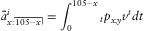$$ \bar{a}_{{x:\left. {\overline{\, {105{\rm{ - }}x} \,}} \!\vskip-1.6pt|\right }}^{i} \: = \:{\int}_{\!\!\!\!0}^{{105{\rm{ - }}x}} {{\,}_t}{{p}_{x,y}}{{v}^t} dt $$

where i is the discount rate, $$$ {{v}^t} \: = \:{{\left( {1\: + \:i} \right)}^{{\rm{ - }}t}} $$$ and _t p_x,y is the probability a life aged x at outset in year y survives for t years:

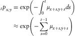$$ no{\quad\quad\quad\quad\quad\quad\quad\quad\quad\quad\quad\quad\quad\quad\quad _{t} {{p}_{x,y}} & \: = \:\exp \left( {{\rm{ - }}{\int}_{\!\!\!\!0}^{t} {{\mu }_{x\: + \:s,y\: + \:s}}ds} \right) \cr & \approx \:\exp \left( {{\rm{ - }}\mathop{\sum}\limits_{s\: = \:0}^{t{\rm{ - }}1} {{\mu }_{x\: + \:s,y\: + \:s}}} \right) $$

2.3 Restricting our calculations to temporary annuities has no meaningful consequences at the main ages of interest, as shown in Table 1.

Table 1

Impact of using a different end age, ω, for the temporary annuity factor $$$ \bar{a}_{{70:\left. {\overline{\, {\omega {\rm{ - }}70} \,}}\!\vskip-1.6pt|\right }}^{{3\% }} $$$. Source: own calculations using S1PA (males) and a discount rate of 3% per annum for cashflows.

For reference, our temporary continuous annuity factors are calculated using the trapezoidal rule for approximating an integral on a uniform grid:

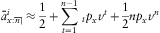$$ \bar{a}_{{x:\left. {\overline{\, n \,}}\! \right| }}^{i} \: \approx \:\frac12\: + \:\mathop{\sum}\limits_{t\: = \:1}^{n{\rm{ - }}1} {{\,}_t}{{p}_x}{{v}^t} \: + \:{{\frac{1}{2}}}n{{p}_x}{{v}^n} $$

2.4 In this paper we will use y = 2011 as a common outset year throughout. From Equations 1 and 2 we will always need a mortality projection for at least (105−x) years to calculate the annuity factor, even if we are only looking for the one-year change in the value of the annuity factor. While we have opted for the temporary-annuity solution, it is worth noting that the models of Cairns et al (Reference Cairns, Blake and Dowd2006) and Richards et al (Reference Richards, Kirkby and Currie2006) are capable of simultaneously extrapolating mortality rates to higher (and lower) ages at the same time as projecting forward in time. These models therefore deserve a special place in the actuarial toolkit, and the subject is discussed in more detail by Richards & Currie (Reference Richards and Currie2011) and Currie (Reference Currie2011).

3. Components of longevity risk

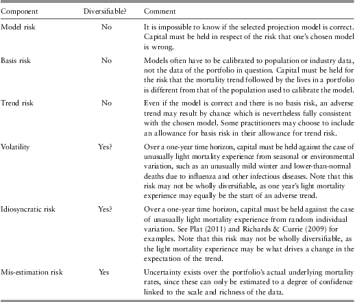
3.1 For high-level work it is often necessary to quote a single capital amount or percentage of reserve held in respect of longevity risk. However, it is a good discipline to itemise the various possible components of longevity risk, and a specimen list is given in Table 2.

Table 2

Specimen itemization of the components of longevity risk. A diversifiable risk can be reduced by growing the size of the portfolio and benefiting from the law of large numbers.

3.2 Table 2 is not intended to be exhaustive and, depending on the nature of the liabilities, other longevity-related elements might appear. In a defined-benefit pension scheme, or in a portfolio of bulk-purchase annuities, there would be uncertainty over the proportion of pensioners who were married, and whose death might lead to the payment of a spouse's pension. Similarly, there would be uncertainty over the age of that spouse. Within an active pension scheme there might be risk related to early retirements, commutation options or death-in-service benefits. Such risks might be less important to a portfolio of individual annuities, but such portfolios would be exposed to additional risk in the form of anti-selection from the existence of the enhanced-annuity market.

3.3 This paper will only address the trend-risk component of Table 2, so the figures in Table 5 and elsewhere can only be minimum values for the total capital requirement for longevity risk. Other components will have to be estimated in very different ways: reserving for model risk requires a degree of subjectivity, while idiosyncratic risk can best be assessed using simulations of the actual portfolio — see Plat (Reference Plat2011) and also Richards & Currie (Reference Richards and Currie2009) for some examples for different portfolio sizes. For large portfolios the idiosyncratic risk will often be diversified away almost to zero in the presence of the other components. In contrast, trend risk and model risk will always remain, regardless of how large the portfolio is. For an overview of how capital requirements for longevity risk fit into the wider regulatory framework, see Makin (Reference Makin2011a, Reference Makin2011b).

4. The stressed-trend approach to longevity risk

4.1 Longevity risk lies in the long-term trend taken by mortality rates. This trend unfolds over many years as an accumulation of small changes, so a natural approach to reserving is to use a long-term stress projection applying over the potential lifetime of the annuitant or pensioner. This view of longevity trend risk is sometimes called the run-off approach, and it does not correspond with the one-year view demanded by a pure value-at-risk methodology. However, the run-off or stressed-trend approach is arguably the most appropriate way to investigate longevity trend risk, and it should therefore not be viewed as invalid merely because it is not a one-year methodology. While a great many insurance risks fit naturally into a one-year value-at-risk framework, not all risks do. It would be excessively dogmatic to insist that longevity trend risk only be measured over a one-year horizon.

4.2 Mortality can be viewed as a stochastic process, as can the direction of mortality trends, so it makes sense to use a stochastic projection model to calibrate a stress trend for longevity risk. This has the benefit of being able to assign a probability to the stress; Figure 1 illustrates the approach. The central projection comes from the maximum-likelihood estimate, while the stress trend is simply the relevant confidence envelope for the central projection. The confidence envelope is derived by multiplying the projection standard error by Φ⁻¹(p), where Φ is the cumulative distribution function of a Normal (0, 1) random variable and p is the relevant probability level (Φ⁻¹(0.005) = −2.58 in this case). Note that the “projection standard error” here encompasses parameter risk, not process risk, and the nature of the projection standard error is discussed in more detail in Section 8. The stressed trend depicted in Figure 1 is smooth because we do not allow for annual volatility in mortality rates, a subject which is discussed in detail in Section 8.

Figure 1

Central projection and stressed trend obtained by deducting 2.58 standard deviations, where $$$ 2.58\: = \:{{\rPhi }^{{\rm{ - }}1}} \left( {99.5\% } \right) $$$. Mortality of males aged 70 in England & Wales, modelled as per Lee & Carter (Reference Lee and Carter1992) with ARIMA(3,1,3) projection of κ_y (see Appendix 1). The ARIMA(3, 1, 3) model was selected from an array of ARIMA(p, d, q) models as having the lowest AIC for this data set

4.3 The stressed-trend approach to longevity risk involves calculating the capital requirement as follows:

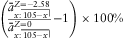$$ \left( {\frac{{\bar{a}_{{x:\:\left. {\overline{\, {105{\rm{ - }}x} \,}}\!\vskip-1.6pt|\right }}^{{Z\: = \:{\rm{ - }}2.58}} }}{{\bar{a}_{{x:\:\left. {\overline{\, {105{\rm{ - }}x} \,}}\!\vskip-1.6pt|\right }}^{{Z\: = \:0}} }}{\rm{ - }}1} \right)\:\times \:100\% $$

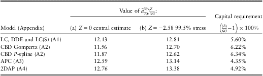
where the numerator with Z = −2.58 denotes the annuity factor calculated with the stressed trend as per Figure 1, and the denominator with Z = 0 denotes the annuity factor calculated with the central projection. The stressed-trend approach behind Figure 1 can be used for a wide variety of regression-type models — Table 3 shows some annuity factors calculated using central estimates and 99.5% stress reserves, together with the resulting capital requirements. Table 3 also illustrates model risk, namely the tendency for different models to produce different central and stressed estimates, and hence different capital requirements.

Table 3

Central and stressed estimates of $$$ \bar{a}_{{70\::\:\left. {\overline{\, {35} \,}}\!\vskip-1.6pt|\right }}^{{3\% }} $$$ from 2011 using models of male mortality applied to data from England & Wales, 1961–2010, ages 50–104. Temporary annuities to age 105 are used to avoid distortions caused by extrapolation to higher ages. All three variants of the Lee-Carter model produced the same values.

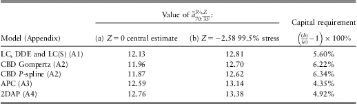
4.4 The stressed-trend capital requirements in Table 3 are dependent on the model, the outset age and the discount rate. Figure 2 shows how the capital requirements vary by age for four different models. Of the models shown, it is interesting to note that the Lee-Carter model yields the second-largest capital requirement up to age 70, but after age 88 it demands the lowest capital requirement. Although the Age-Period-Cohort model generates consistently low capital requirements, Currie (Reference Currie2012) raises concerns about the assumptions required in projecting mortality using the APC model.

Figure 2

Capital requirement at age x on valuation date for $$$ \bar{a}_{{x\::\:\left. {\overline{\, {105{\rm{ - }}x} \,}}\!\vskip-1.6pt|\right }}^{{3\% }} $$$ from stressed trend at 99.5% level for four of the models in Table 3. Graph shows the capital requirement defined in Equation 4 for varying outset ages. The different patterns by annuity outset age show the importance of selecting a specimen age which represents the portfolio for which capital requirements are being calculated. Different models show different patterns by age in part because they vary in the extent to which mortality rates are correlated under each model.

4.5 There is also the question of how best to measure the impact of longevity risk. Plat (Reference Plat2011) carries out a whole-portfolio valuation to minimise the risks associated with representing a portfolio with model points, which makes the published results portfolio-specific. In contrast, we have often chosen a single specimen age for most calculations in this paper on the grounds of simplicity, although in practice for a given portfolio it would be better to follow the approach of Plat (Reference Plat2011). As to the choice of specimen age, Börger (Reference Börger2010) chose age 65 to illustrate the impact of different interest rates, and this age would generally be appropriate for newly written annuity business. In contrast, we have chosen age 70 as it is more likely to be representative of mature portfolios of pensions in payment (i.e. excluding deferred or active members in a pension scheme).

4.6 Another important feature is the sensitivity of the capital requirement to the rate of discount. Börger (Reference Börger2010) notes that capital requirements increase as the (net) discount rate decreases. Figure 3 shows the stressed-trend capital requirements under the Lee-Carter model, which show that lower discount rates lead to higher capital requirements. Interest rates are particularly low at the time of writing, so the presence of significant volumes of escalating annuities could mean an effective net discount rate close to zero for some portfolios. Indeed, interest rates are not only low but the yield curve has a very particular shape which has some consequences of its own (see Appendix A6).

Figure 3

Capital requirement by age for $$$ {{\bar{a}}_{x:\left. {\overline{\, {105{\rm{ - }}x} \,}}\!\vskip-1.6pt|\right }} $$$ from stressed trend at 99.5% level. Graph shows the capital requirement defined in Equation 4 for varying outset ages and using various discount rates. Mortality is according to the Lee-Carter model from Table 3.

4.7 One consequence of the stressed-trend approach is that, for a given p-value, it will tend to produce higher capital requirements than a one-year approach. Some practitioners use a simple approach to try and allow for this by picking a p-value for the stressed-trend which is less than the 99.5th percentile required for the one-year approach. However, this can be arbitrary, and even less subjective approaches can be inconsistent. For example, one simple approach might be to select a p-value, p, such that 0.995ⁿ = 1 − p. The parameter n could be chosen relative to the portfolio under consideration, say by setting it to the discounted mean term of the annuity payments. However, the drawback of this approach is that portfolios exposed to greater levels of longevity risk will receive less onerous values of p. For example, assume n = 10 for a portfolio of level annuities, thus leading to p = 0.0489. If we then assume that the annuities are in fact escalating, the value of n might increase to 12 (say), leading to p = 0.0631. This is counter-intuitive — the portfolio of escalating annuities is arguably more exposed to longevity risk, so why should it be subjected to a weaker stress scenario? Deriving a one-year longevity stress from a multi-year calculation is tricky, and so other methodologies are required.

5. The shock approach to longevity risk

5.1 A simplified standard-formula approach to longevity risk is to assume an immediate fall in current and future projected mortality rates, i.e.

$$\mu _{{x,t}}^{{{\rm{shock}}}} \: = \:{{\mu }_{x,t}}\:\times \:\left( {1{\rm{ - }}f} \right)$$

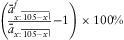
where μ_x,t is the central mortality projection (Z = 0) behind Table 3 and f is the shock reduction in mortality rates. Analogous to Equation 4, the shock capital requirements are:

$$ \left( {\frac{{\bar{a}_{{x:\left. {\overline{\, {105{\rm{ - }}x} \,}}\!\vskip-1.6pt|\right }}^{f} }}{{{{{\bar{a}}}_{x:\left. {\overline{\, {105{\rm{ - }}x} \,}}\!\vskip-1.6pt|\right }}}}{\rm{ - }}1} \right)\:\times \:100\% $$

where the numerator is the annuity factor calculated with the shocked mortality rates according to Equation 5 and the denominator is the annuity factor calculated using the central projection. The QIS5 rules for Solvency II specify f = 20% (European Commission, 2010), and the results of this are shown in Figure 4 for the Lee-Carter model from Table 3. It is worth noting that the shock approach is designed to cover more aspects of longevity risk than just the trend risk. The subject of the various components of longevity risk is addressed in Section 2.

5.2 The standard-formula approach conflicts with the stressed-trend approach: whereas in Figure 2 the capital requirements reduce after around age 70, the standard-formula capital requirements increase steadily with age to reach excessive levels. Furthermore, the capital requirements at younger ages look to be a little too low compared with the stressed-trend approach of Figure 2. Any given portfolio contains many pensions at different ages, of course, and the appropriateness (or otherwise) of the shock approach depends on the individual portfolio. Richards & Currie (Reference Richards and Currie2009) suggested that it might be reasonable for a new and growing annuity portfolio.

5.3 The stressed-trend approach produces a more intuitive set of results than the shock approach — capital requirements are greater at younger ages, where there is more scope for suffering from an adverse long-term trend. Furthermore, comparing Figures 4 and 2 suggests that the stressed-trend approach produces lower capital requirements than the shock approach. Börger (Reference Börger2010) describes “the structural shortcomings of the shock (approach)”, specifically the too-low capital requirements at younger ages and the too-high requirements at older ages, concluding that “an age-dependent stress with smaller reductions for old ages might be more appropriate”. In theory this might not matter, as the shock approach would be intended to work at a portfolio level and excess capital at higher ages would be offset by lower capital requirements at younger ages, although whether this worked in practice would depend critically on the profile of liabilities by age. Also, the shock approach, as structured as a standard formula under Solvency II, is intended to cover more than just longevity trend risk.

Figure 4

Capital requirement by age for $$$ \bar{a}_{{x:\left. {\overline{\, {105{\rm{ - }}x} \,}}\!\vskip-1.6pt|\right }}^{{3\% }} $$$ from an immediate fall in mortality rates of 20%. Graph shows capital requirements calculated according to Equation 6 using f = 0.2 and the central Lee-Carter projection in Figure 1 (Z = 0).

6. A Value-at-Risk framework

6.1 The stressed-trend approach of Section 4 deals with changes in mortality rates over many years. This does not answer the one-year value-at-risk question, so something different is needed for the likes of Solvency II. This Section describes a one-year framework for longevity risk based on the sensitivity of the central projection to new data. This approach differs from the models of Börger (Reference Börger2010) and Plat (Reference Plat2011), which seek to model the trend and its tail distribution directly. Börger (Reference Börger2010) and Plat (Reference Plat2011) also present specific models, whereas the framework described here is general and can accommodate a wide range of stochastic projection models. In contrast to Plat (Reference Plat2011), who modelled longevity risk and insurance risk, the framework here is intended to focus solely on longevity trend risk in pensions and annuities in payment.

6.2 At a high level we use a stochastic model to simulate the mortality experience of an extra year, and then feed this into an updated model to see how the central projection is affected. This is repeated many times to generate a probability distribution of how the central projection might change over a one-year time horizon. In more detail the framework is as follows:

6.3 First, select a data set covering ages x_L to x_H and running from years y_L to y_H. This includes the deaths at each age in each year, d_x,y, and the corresponding population exposures. The population exposures can be either the initial exposed-to-risk, E_x,y or the mid-year central exposed-to-risk, $$$ E_{{x,y}}^{c} $$$. For this process we need the exposures for the start of year y_{H + 1}, so if the basic exposures are central we will approximate the initial exposures using $$$ {{E}_{x,{{y}_{H\: + \:1}}}}\: \approx \:E_{{x{\rm{ - }}1,{{y}_H}}}^{c} {\rm{ - }}{{d}_{x{\rm{ - }}1,{{y}_H}}}/2 $$$.

6.4 Next, select a statistical model and fit it to the data set in ¶6.3. This gives fitted values for logμ_x,y, where x is the age in years and y is the calendar year. We can use the projections from this model to calculate various life expectancies and annuity factors at specimen ages if desired.

6.5 Use the statistical model in ¶6.4 to generate sample paths for $$$ \log {{\mu }_{x,{{y}_{H\: + \:1}}}} $$$, i.e. for the year immediately following the last year for which we have data. These sample paths can include trend uncertainty or volatility or both (see Section 8). In practice the dominant source of uncertainty over a one-year horizon is usually volatility, so this should always be included. We can estimate $$$ {{q}_{x,{{y}_{H\: + \:1}}}} $$$, the binomial probability of death in year y_{H + 1}, by using the approximation $$$ q\: \approx \:1{\rm{ - }}{{e}^{{\rm{ - }}\mu }} $$$.

6.6 We simulate the number of deaths in year y_{H + 1} at each age as a binomial random variable. The population counts are the $$$ {{E}_{x,{{y}_{H\: + \:1}}}} $$$ from ¶6.3 and the binomial probabilities are those simulated in ¶6.5. This gives us simulated death counts at each age apart from x_L, and we can calculate corresponding mid-year exposures as $$$ E_{{x,{{y}_{H\: + \:1}}}}^{c} \: \approx \:{{E}_{x,{{y}_{H\: + \:1}}}}{\rm{ - }}{{d}_{x,{{y}_{H\: + \:1}}}}/2 $$$.

6.7 We then temporarily append our simulated data from ¶6.6 to the real data in ¶6.3, creating a single simulation of the data we might have in one year's time. The missing data for age x_L in year y_{H + 1} is treated by providing dummy values and assigning a weight of zero. We then refit the statistical model to this combined data set, reperform the projections and recalculate the life expectancies and annuity values at the specimen ages using the updated central projection.

6.8 Repeat steps ¶6.5 to ¶6.7 n times, where n might be at least 1,000 (say) for Solvency II-style work. It is implicit in this methodology that there is no migration, or that if there is migration its net effect is zero, i.e. that immigrants have similar numbers and mortality characteristics to emigrants. The choice of n will have a number of practical considerations, but for estimating the 99.5th percentile a minimum value of n = 1,000 is required.

6.9 Figure 5 shows the resulting updated central projections from a handful of instances of performing steps ¶6.3–¶6.8. Note that we do not require nested simulations, as the central projection is evaluated without needing to perform any simulations. The nature of projections and their standard errors is discussed in Section 8.

Figure 5

One-year approach to longevity risk. Experience data for 2011 are simulated using sample paths from an ARIMA(3, 1, 3) process and the Lee-Carter model is refitted each time the 2011 data are simulated. The changes in central projections give an idea of how the best estimate could change over the course of a year based on new data. For comparison with Figure 1, all of the projections here are Z = 0. Although we are interested in the one-year change in annuity factor, we have to do a full multi-year projection in order to have projected mortality rates to calculate the annuity factor in Equation 1.

6.10 After following this procedure we have a set, S, of n realised values of how life expectancies or annuity values can change based on the addition of a single year's data:

$$ S\: = \:\{ \bar{a}_{x}^{j} ;j\: = \:1,2, \ldots, n\} $$

6.11 S can then be used to set a capital requirement to cover potential changes in expectation of longevity trend risk over one year. For example, a one-year value-at-risk estimate of trend-risk capital would be:

$$ \left( {\frac{{{\rm{9}}{{{9.5}}^{{\rm{th}}}} \;{\rm{percentile}}\;{\rm{of}}\;S}}{{{\rm{mean}}\;{\rm{of}}\;S}}{\rm{ - }}1} \right)\:\times \:100\% $$

6.12 Appendix 5 contains details of how percentiles are estimated from sets of data in this paper. Before we come to the results of this approach in Section 9, we must first consider which models are appropriate (Section 7) and how to generate sample paths (Section 8).

7. Model choices

7.1 Suitable models for the framework in Section 6 are those which are (i) estimated from data only, i.e. regression-type models where no subjective intervention is required post-fit, and (ii) are capable of generating sample-path projections. Most statistical projection models are therefore potentially suitable, including the Lee-Carter family (Appendix 1), the Cairns-Blake-Dowd model (Appendix 2), the Age-Period-Cohort model (Appendix 3) and 2D P-spline model (Appendix 4). This is by no means an exhaustive list, and many other models could be used. Note that a number of models will be sensitive to the choice of time period (i.e. y_L to y_H) and some models will be sensitive to the choice of age range (i.e. x_L to x_H).

7.2 Unsuitable models are those which either (i) require parameters which are subjectively set, or which are set without reference to the basic data, or (ii) are deterministic scenarios. For example, the CMI's 2009–2011 models cannot easily be used here because they are deterministic targeting models which do not generate sample paths — see CMI (2009, 2010). Models which project mortality disaggregated by cause of death could potentially be used, provided the problems surrounding the projection of correlated time series were dealt with — see Richards (Reference Richards2010) for details of other issues with cause-of-death projections. Models which contain artificial limits on the total possible reduction in mortality would not be suitable, however, as the purpose of this exercise is to estimate tail risk. When modelling tail risk, it would be self-defeating to use a model which starts by limiting the tail in question. In addition to this, Oeppen & Vaupel (Reference Oeppen and Vaupel2004) show that models claiming to know maximum life expectancy (and thus limiting the maximum possible improvements) have a poor record.

8. Sample paths

8.1 The framework in Section 6 requires the generation of sample-path projections for the following year. There are two components to the uncertainty over projected mortality rates: (i) trend risk, and (ii) volatility. Trend risk is the uncertainty over the general direction taken by mortality rates, and is what is illustrated in Figure 1. Trend uncertainty is determined by the uncertainty over the parameters in the projection model, and is therefore a form of parameter risk. Volatility is an additional risk on top of the particular direction taken — it arises due to temporary fluctuations in mortality around the trend, such as those caused by a harsh (or mild) winter, or an outbreak of influenza. Volatility is fundamentally a short-term phenomenon and would therefore seem to be of less concern to an annuity writer than the trend risk. However, volatility plays an important role in the one-year simulations required for the framework described in Section 6.

8.2 The distinction between trend risk and volatility can be illustrated by examining a drift model, which says that the mortality index κ in year y + 1 is related to the index in the previous year by the simple relationship:

$$ {{\kappa }_{y\: + \:1}}\: = \:{{\kappa }_y}\: + \:{\rm{drift}}\;{\rm{constant}}\: + \:∈_{\!y\: + \:1}} $$

where κ_y is (say) the Lee-Carter mortality index in year y and {∈_y} is a set of independent, identically distributed noise terms with zero mean and variance $$$ \sigma _{ \in }^{2} $$$. In fitting a drift model there are therefore three parameters to be estimated: (i) the drift constant, (ii) the standard error of the drift constant, σ _drift, and (iii) the standard error of the noise process, σ_∈. For an annuity writer, trend risk lies in the uncertainty over the drift constant, i.e. in the parameter risk expressed by σ _drift. For an assurance-type liability the situation may be reversed and the dominant risk might be the noise variance, σ_∈, i.e. the volatility.

8.3 For a detailed risk investigation any simulation should be capable of including or excluding each type of risk independently, i.e. (i) trend risk only, (ii) volatility only, and (iii) trend risk and volatility combined. This enables the actuary to not only reproduce a realistic-looking sample-path projection when required, but also to test the relative contribution of each of the two risks to the costs for a given liability profile.

8.4 The drift model in Equation 9 is a simple and restricted subset of a full ARIMA model for κ_y. The situation for simulations under ARIMA models is analogous: there is a noise process as before, but now κ_{y + 1} is related to one or more previous values as an autoregressive moving average. There are therefore more parameters to be estimated than just the drift constant, and each new parameter will also have an estimated standard error corresponding to σ _drift. As before, the variance of the noise process, $$$ {\rm{\sigma }}_{∈}^{2} $$$, will be labelled as the volatility, while the trend risk lies in the standard error of $$$ \log {{\hat{\mu }}_{x,y}} $$$, which arises from the uncertainty surrounding the various ARIMA parameter estimates.

8.5 For models projecting via a penalty function the situation is different because the forecast is always smooth and there is no volatility. However, simulation of volatility can be achieved by randomly sampling columns from the matrix of unstandardised residuals and adding them column-wise to the smooth projection. This approach is very general and requires no distributional assumption for the volatility — and therefore no estimate of σ_∈ — as the empirical set of past volatility is used for sampling. This has the advantage of simulating mortality shocks in a given year while preserving the age structure. For any smooth projection model, therefore, a simulated sample path, $$$ \mu _{{x,y}}^{{{\rm{simulated}}}} $$$, can be obtained as follows:

$$ \log \mu _{{x,y}}^{{{\rm{simulated}}}} \: = \:\log {{\hat{\mu }}_{x,y}}\: + \:Z{{\sigma }_{x,y}}\: + \:I{{r}_{x,y}} $$

where $$$ {{\hat{\mu }}_{x,y}} $$$ is the smooth projected force of mortality and σ_x,y the corresponding standard error of $$$ \log {{\hat{\mu }}_{x,y}} $$$. Z is a value from a N(0, 1) distribution, while I is an indicator variable taking the value zero (if excluding volatility) or one (if including volatility). r_x,y is derived from a randomly chosen column j from the unstandardised residuals thus:

$$ {{r}_{x,y}}\: = \:\log {{D}_{x,j}}{\rm{ - }}\log E_{{x,j}}^{c} {\rm{ - }}\log {{\hat{\mu }}_{x,j}} $$

where j is a year in the data region, i.e. $$$ j\, \in \,\{ 1961,1962, \ldots, 2010\} $$$ for the data in this paper, and y ≥ 2011. With this method of simulating sample paths for smooth projection models, we again have the facility to consider the two components of risk in Equation 10 either separately or combined. To include trend risk only, we sample Z from a N(0, 1) distribution and set I = 0. To include volatility only, we set Z = 0 and I = 1. To include both trend risk and volatility, we sample Z from N(0,1) and set I = 1. Note that this approach will work for any model where projections are smooth, including the fully smoothed 2D P-spline models of Richards et al (Reference Richards, Kirkby and Currie2006) and the variant of the Lee-Carter model in Richards & Currie (Reference Richards and Currie2009).

8.6 Although we have very different structures for our projections — drift models, ARIMA processes and penalty forecasts — we can nevertheless arrange a common framework for trend risk (represented by parameter uncertainty) and volatility (which is either simulated or resampled from the past departure from the model fit). These two separate components are individually switchable to allow investigation of their respective and combined impact. This is summarised in Table 4.

Table 4

Sources of uncertainty in sample paths

8.7 There is an irony behind Table 4 and the VaR approach to longevity risk. Longevity risk is essentially about an adverse long-term trend, the uncertainty about which is predominantly described by parameter risk. However, when simulating over a time horizon as short as a year, the volatility is likely to play the major role.

9. Results of the one-year VaR approach

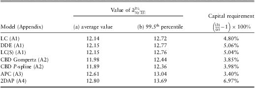
9.1 The framework in Section 6 is applied to some of the models in Table 3. The results for some selected models are shown in Table 5. As a check, the average annuity value in column (a) in Table 5 should be very close to the central annuity value in column (a) in Table 3.

Table 5

Average and 99.5^th percentile values for $$$ \bar{a}_{{70:\left. {\overline{\, {35} \,}}\!\vskip-1.6pt|\right }}^{{3\% }} $$$ from 2011 using models of male mortality applied to data from England & Wales, 1961–2010, ages 50–104. Temporary annuities to age 105 are used to avoid distortions caused by extrapolation to higher ages. Discounting is at 3% per annum. Percentiles are estimated using the method described in Appendix 5. Results are based on 1,000 simulations according to the procedure described in steps ¶6.3–¶6.8.

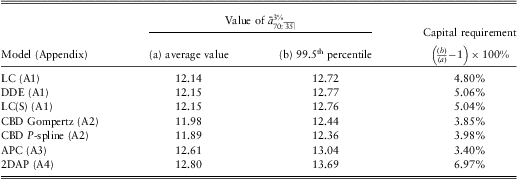
9.2 With the exception of the 2DAP, the capital requirements shown in Table 5 are lower than the equivalent values in Table 3. This is partly because the data behind the models in Table 3 end in 2010 and project rates forward to 2011 and beyond. In contrast, the data behind the models in Table 5 end in 2011 due to the simulated extra year's experience, so there is one year's less uncertainty in the projections. However, the primary driver in the reduced capital requirements in Table 5 is the difference in time horizon — a single year as opposed to the run-off in Table 3. As with Table 3, model risk is illustrated by the varying capital requirements.

9.3 One issue with the Figures in Table 5 is that they are sample quantiles, i.e. they are based on the top few order statistics and are therefore themselves random variables with uncertainty surrounding their estimated value. One approach is to use a more sophisticated estimator of the quantile, such as that from Harrell & Davis (Reference Harrell and Davis1982). Such estimators are more efficient and produce standard errors for the estimator without any distributional assumptions. Figure 6 illustrates the Harrell-Davis estimates of the value-at-risk capital for the smoothed Lee-Carter model, LC(S), together with a confidence envelope around those estimates.

Figure 6

Harrell-Davis (Reference Harrell and Davis1982) estimate of 99.5% value-at-risk capital requirement for LC(S) model in Table 5, together with approximate 95% confidence envelope.

9.4 Plat (Reference Plat2011) felt that there was a risk of underestimation of true risk if the so-called spot model is not responsive to a single extra year's experience. This is perhaps true of the time-series models shown in Table 5. However, this cuts both ways as overestimation of capital requirements is also possible if the model is too responsive. This is possible for models using penalty projections, such as those of Richards et al (Reference Richards, Kirkby and Currie2006) and Richards & Currie (Reference Richards and Currie2009), and an illustration of what can go wrong is given in ¶10.3.

10. A test for model robustness

10.1 Besides answering the value-at-risk question, the framework outlined here can also be used to test a model for robustness to new data. When selecting a model for internal management use, it is important to know two things about its behaviour when new data becomes available. First, one wants the model to fit, and second, one wants the model to produce sensible results. For example, Richards et al (Reference Richards, Ellam, Hubbard, Lu, Makin and Miller2007) highlight occasions when two-dimensional P-spline models can come unstuck due to under-smoothing in the time direction. A particular model must be tested in advance to see if it is vulnerable to such behaviour and either correct it or choose a different model.

10.2 Note that the question of robustness here — will the model fit and work? — is quite different from the question of model suitability, which might itself be addressed by back-testing or the kind of quantitative assessment carried out by Cairns et al (Reference Cairns, Blake, Dowd, Coughlan, Epstein, Ong and Balevich2009). Indeed, the one-year framework presented in this paper might usefully be added to the tests in Cairns et al (Reference Cairns, Blake, Dowd, Coughlan, Epstein, Ong and Balevich2009) when considering an internal model. To illustrate, consider the models listed in Table 5. In each case 1,000 simulations were carried out of the next year's potential mortality experience, and in each case the model was successfully refitted. The resulting capital requirements are in a similar enough range to conclude that any one of these models could be used as an internal model, safe in the knowledge that once the commitment has been made to use the model the user is unlikely to be surprised by the model's response to another year's data.

10.3 In contrast, consider an example where we remove the over-dispersion parameter from the 2DAP model, i.e. we force ψ ² = 1 regardless of the over-dispersion apparent in the data (see Appendix 4 for details of the over-dispersion parameter). With 1,000 simulations of the framework in steps ¶6.3 to ¶6.8, there were five instances where the model without over-dispersion could not fit. Although this failure rate sounds small (0.5%), the implied capital requirement is also of the order of 30%. When the model fits are inspected, we see that a number of the simulations have led to under-smoothing in time and thus excessively volatile projections. The 2DAP model is therefore only usable as an internal model with the England & Wales dataset with the over-dispersion parameter. Analogous situations are possible with many other models, and it is obviously important to find a model's weak points before committing to use it.

10.4 The procedure described in steps ¶6.3–¶6.8 is therefore not only useful for value-at-risk calculations, it is also a practical test of the robustness of a model. The procedure can be used to check that the model selected this year will continue to perform sensibly when new data arrive next year. Furthermore, there is no reason to force the generating stochastic model to be the same as the one being tested. The reality of model risk — as shown in Tables 3 and 5 — means that a thorough robustness test would involve testing a model's ability to handle the sample paths generated by a different model. Without this sort of test, there is a risk of investing in a given model only for it to surprise (or embarrass) when new data become available. It therefore makes sense to throughly test a model before committing to using it.

11. Conclusions

11.1 There are a number of components to longevity risk, of which trend risk is just one part. The longevity trend risk faced by insurers and defined-benefit pension schemes exists as a long-term accumulation of small changes, which could together add up to an adverse trend. Despite the long-term nature of longevity risk, there are reasons why insurers and others want to look at longevity through a one-year, value-at-risk prism. These reasons include the one-year horizon demanded by the ICA regime in the United Kingdom and the pending Solvency II regime for the European Union. This paper describes a framework for putting a long-term longevity trend risk into a one-year view for setting capital requirements. The results of using this framework tend to produce lower capital requirements than the stressed-trend approach to valuing longevity risk, but this is not uniformly the case.

11.2 Whatever the choice of method — stressed trend, mortality shock or value-at-risk — the actual capital requirements depend on the age and interest rate used in the calculations, and also the choice of model. However, the three approaches used in this paper suggest that, at a specimen male age of 70 and based on population mortality rates, the capital requirement in respect of longevity trend risk in level annuities should be at least $$${\rm{3}}\frac{{\rm{1}}}{{\rm{2}}}\% $$$ of the best-estimate reserve. For escalating annuities, or for indexed pensions in payment, the minimum capital requirement in respect of longevity trend risk will be higher.