1 Introduction
Vortex cavitations emerge frequently in marine hydrofoils, propellers and turbomachinery. At the tip of a blade, a vortex is generated from the rolling up of liquid to the lifting surface. If the vortex circulation is sufficiently large, the pressure in the core of the vortical flow can decrease to the saturated vapour pressure, and cavitation occurs therefrom. The oscillation and breakup of a vortex cavitation bubble are responsible for a broad frequency range of noise (McCormick Reference McCormick1962; Arndt Reference Arndt2002). These noises will impact the environment in different circumstances. For example, ocean ambient noise of low frequency (10–500 Hz) may overlap and mask the communication frequency band of marine mammals and hence adversely affect their fundamental living activities (Hildebrand Reference Hildebrand2009). Moreover, noise is vital to the survivability of a naval ship and significant to the comfort of a commercial ship. The acoustic signature from tip vortex cavitation is one of the most crucial sources of noise.
The noise generated from vortex cavitation is highly associated with the dynamics of cavitating bubbles embedded in tip vortex regions. The peak in the noise spectrum was found to be accompanied with the appearance of a standing wave on the surface of a hollow vortex core (Maines & Arndt Reference Maines and Arndt1997). Peng et al. (Reference Peng, Wang, Li, Xu and Song2017) figured out that the frequency of an abnormal acoustic noise matches the fundamental natural frequency of the cavitating tip vortex bubble. Various scaling laws, which were proposed to predict the vortex cavitation noise from laboratory scale to prototype scale, rely on the knowledge of the physical mechanism of oscillation of the tip vortex cavitation (Levkovskii Reference Levkovskii1968; Blake, Wolpert & Geib Reference Blake, Wolpert and Geib1977; Bark Reference Bark1985; Oshima Reference Oshima1990; Shen, Gowing & Jessup Reference Shen, Gowing and Jessup2009; Park & Seong Reference Park and Seong2017). Therefore, an effective inhibition of cavitation noise requires a full understanding of the dynamics of a vortex cavitation bubble.
The inception of vortex cavitation involves explosive growth of small nuclei or bubbles. This process happens within
 $1~\unicode[STIX]{x03BC}\text{s}$
(Franc & Michel Reference Franc and Michel2010), pushing the surrounding fluid rapidly outwards. Owing to the conservation of angular momentum, the rotational velocity at the interface reduces along with the increase of radius. Consequently, the liquid pressure at the interface increases and suppresses the growth of the cavitation bubble. Until the radial motion decelerates to zero, the bubble begins to shrink, accompanied with an increase in rotational velocity and thus a decrease in the nearby pressure. In this way, an oscillation in radial direction takes place. In quiescent water, air nuclei of tens of micrometres are usually spherical. When these spherical bubbles are entrapped by the tip vortex, corresponding to vortex cavitation inception, they will fill in the core of the vortex and grow primarily along the vortex trajectory. Therefore, a cylindrical bubble is an ideal and suitable model to represent a highly elongated bubble.
The dynamic equation of the radial oscillation for a cylindrical bubble can be described by the Rayleigh–Plesset type equation, established through integrating the radial Euler equation (Chahine Reference Chahine1995). Additional effects, such as compressibility (Roberts Reference Roberts2003; Ilinskii et al. Reference Ilinskii, Zabolotskaya, Hay and Hamilton2012) or a neighbouring bubble (Quinto-Su & Ohl Reference Quinto-Su and Ohl2009), were added in the subsequent models. For elongated cavitation bubbles, the oscillatory period depends on the circulation of the vortex and the radius of the bubble (Choi et al. Reference Choi, Hsiao, Chahine and Ceccio2009), which can be applied for bubbles in a single vortex (Choi & Ceccio Reference Choi and Ceccio2007) and more complex stretched vortices (Chang & Ceccio Reference Chang and Ceccio2011). The experiment conducted by Choi & Ceccio (Reference Choi and Ceccio2007) revealed comprehensive effects, including free-stream conditions and vortex properties. Considering the limitation of model scales in the experiment, their group performed numerical simulations and found that the bubble dynamics are highly sensitive to flow parameters (Choi et al. Reference Choi, Hsiao, Chahine and Ceccio2009). This makes the prediction of the dynamics of a vortex cavitation bubble challenging even when only considering the radial variation.
The wave-like surface mode is a key feature in the dynamics of a vortex cavitation bubble. The wave propagation on a hollow irrotational vortex in a cylindrical tube was studied first by Thomson (Reference Thomson1880), in which the general dispersion relationship for each surface mode restored by centrifugal forces was derived. Surface modes of a tip-vortex cavitation bubble were observed on various hydrofoils in cavitation experiments (Arndt, Arakeri & Higuchi Reference Arndt, Arakeri and Higuchi1991; Pennings et al. Reference Pennings, Bosschers, Westerweel and van Terwisga2015; Peng et al. Reference Peng, Wang, Li, Xu and Song2017). We are interested in the evolution of the surface mode and its stability under specific flow conditions.
The occurrence of a surface mode for a cylindrical cavitation bubble may be analogous to that for a spherical bubble, which has been studied extensively in the literature (see the review papers by Plesset & Prosperetti (Reference Plesset and Prosperetti1977) and Feng & Leal (Reference Feng and Leal1997)). The instability of a spherical interface can be stimulated by the Rayleigh–Taylor instability or the Mathieu-type instability. The former happens when a light fluid accelerates towards a heavy one, e.g. when the bubble reaches its minimal size and rebounds. The latter is substantially relevant to the energy transfer from the radial mode to the surface mode when their oscillations resonate according to the Mathieu relation. The time scales of these two instabilities are quite different – at a shorter time scale of the order of nanoseconds for the Rayleigh–Taylor instability and a longer time scale comparable with the radial oscillation period for the Mathieu-type instability (Hilgenfeldt, Lohse & Brenner Reference Hilgenfeldt, Lohse and Brenner1996).
By comparison, the surface stability of a cylindrical bubble has received less attention. Pennings et al. (Reference Pennings, Bosschers, Westerweel and van Terwisga2015) derived a dispersion relation for the surface mode based on a potential flow and validated it by their experiment, which established fundamental knowledge on the kinematics of various surface modes. Vadivukkarasan & Panchagnula (Reference Vadivukkarasan and Panchagnula2017) analysed the mechanism of Rayleigh–Taylor instability at a cylindrical interface. To investigate the mechanism of generation and energy transfer, and the corresponding stability for each surface mode, we formulate dynamic equations by studying an initial value problem for a cylindrical cavitation bubble, so that the temporal development of surface modes can be predicted. The amplitudes of surface modes are assumed to be small compared with that of the radial mode, which permits the use of perturbation methods. In addition, we derive the Mathieu structure in the dynamic equation of surface modes and demonstrate the possibility of the Mathieu-type instability developing in a cylindrical cavitation bubble. We incorporate viscous effects on the interface in order to complete the model and the stability analysis. Considering that the vortex cavitation is generated in a water tunnel, we also take into account the effect of confinement on the surface mode.
The rest of the paper is organized as follows. In § 2, we derive the dynamic equations for the surface oscillation of a vortex cavitation bubble without/with confinement and viscosity. The effects of gas pressure, confinement and viscosity are evaluated in §§ 3.1, 3.2 and 3.3, respectively. In § 3.4, our model is validated by comparison with the experimental results of Pennings et al. (Reference Pennings, Bosschers, Westerweel and van Terwisga2015). In § 3.5, the Mathieu structure is derived from our model equation and an instability condition is obtained. In § 3.6, the developments of surface modes demonstrate the existence of Mathieu-type instability. Finally, concluding remarks are given in § 4.
2 Problem formulation
2.1 Geometry of a cylindrical bubble
We consider a vortex cavitation bubble with infinite length and establish a cylindrical coordinate system
 $(r,\unicode[STIX]{x1D703},z)$
, where
 $(r,\unicode[STIX]{x1D703})$
is parallel to the cross-section of the bubble and the
 $z$
-coordinate is along the longitudinal direction. The radial coordinate at the bubble interface
 $r_{c}$
is composed of a mean radius
 $R_{c}$
and a distortion to a cylindrical shape,
 $$\begin{eqnarray}r_{c}(\unicode[STIX]{x1D703},z,t)=R_{c}(t)+\unicode[STIX]{x1D700}\mathop{\sum }_{m=0}^{\infty }a_{m}(t)\text{e}^{\text{i}(kz+m\unicode[STIX]{x1D703})}\quad (\unicode[STIX]{x1D700}\ll 1),\end{eqnarray}$$
where
 $a_{m}$
is the amplitude of the surface mode,
 $k$
is the wavenumber in the
 $z$
-direction and
 $m$
is the azimuthal wavenumber in the
 $\unicode[STIX]{x1D703}$
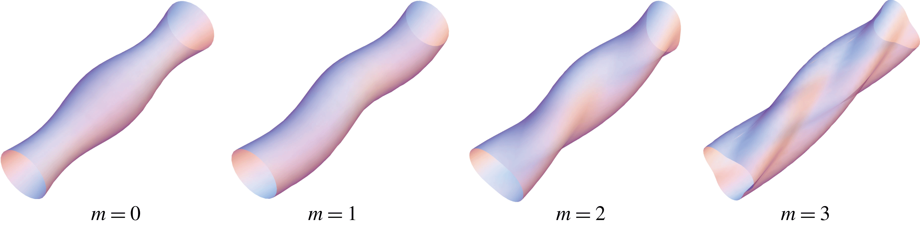
-direction. The shapes of the surface modes for
 $m=0$
, 1, 2 and 3 have been given in Thomson (Reference Thomson1880) and are re-illustrated in figure 1. The actual shape of a bubble is the superposition of different modes. In this paper, we only consider the decoupled dynamic equation for the surface mode under linear analysis, and the terms of order higher than
 $O(\unicode[STIX]{x1D700})$
are hence eliminated. For the sake of conciseness, the summation notation in (2.1) is omitted in the following. The surface shape function is defined as
 $$\begin{eqnarray}S(r,\unicode[STIX]{x1D703},z;t)\doteq r-R_{c}(t)-\unicode[STIX]{x1D700}a_{m}(t)\text{e}^{\text{i}(kz+m\unicode[STIX]{x1D703})}=0,\end{eqnarray}$$
from which we derive the unit normal vector
 $\boldsymbol{n}$
and the total curvature of the bubble surface
 $\unicode[STIX]{x1D735}\boldsymbol{\cdot }\boldsymbol{n}$
:
 $$\begin{eqnarray}\boldsymbol{n}=\frac{\unicode[STIX]{x1D735}S}{|\unicode[STIX]{x1D735}S|}=\boldsymbol{e}_{r}+\boldsymbol{e}_{\unicode[STIX]{x1D703}}\frac{1}{r}\frac{\unicode[STIX]{x2202}S}{\unicode[STIX]{x2202}\unicode[STIX]{x1D703}}+\boldsymbol{e}_{z}\frac{\unicode[STIX]{x2202}S}{\unicode[STIX]{x2202}z},\end{eqnarray}$$
 $$\begin{eqnarray}\displaystyle \unicode[STIX]{x1D735}\boldsymbol{\cdot }\boldsymbol{n} & = & \displaystyle \frac{1}{r}\frac{\unicode[STIX]{x2202}S}{\unicode[STIX]{x2202}r}+\frac{1}{r}\frac{\unicode[STIX]{x2202}}{\unicode[STIX]{x2202}\unicode[STIX]{x1D703}}\left(\frac{1}{r}\frac{\unicode[STIX]{x2202}S}{\unicode[STIX]{x2202}\unicode[STIX]{x1D703}}\right)+\frac{\unicode[STIX]{x2202}}{\unicode[STIX]{x2202}z}\left(\frac{\unicode[STIX]{x2202}S}{\unicode[STIX]{x2202}z}\right)\nonumber\\ \displaystyle & = & \displaystyle \frac{1}{R_{c}}+\unicode[STIX]{x1D700}(m^{2}+k^{2}R_{c}^{2}-1)\frac{a_{m}}{R_{c}^{2}}\text{e}^{\text{i}(kz+m\unicode[STIX]{x1D703})}.\end{eqnarray}$$
The variation of a cylindrical bubble volume per unit length is calculated to be
 $$\begin{eqnarray}\frac{V_{c}(t)}{V_{c0}}=\frac{1}{\unicode[STIX]{x03C0}R_{c0}^{2}}\int _{0}^{2\unicode[STIX]{x03C0}}\frac{r_{c}^{2}}{2}\,\text{d}\unicode[STIX]{x1D703}=\frac{R_{c}^{2}}{R_{c0}^{2}}+2\unicode[STIX]{x1D700}\frac{R_{c}a_{0}}{R_{c0}^{2}}+\unicode[STIX]{x1D700}^{2}\frac{a_{0}^{2}}{R_{c0}^{2}}+\unicode[STIX]{x1D700}^{2}\mathop{\sum }_{m=1}^{\infty }\frac{a_{m}^{2}}{2R_{c0}^{2}},\end{eqnarray}$$
where
 $V_{c}$
is the instantaneous volume of the bubble, and
 $R_{c0}=R_{c}(0)$
and
 $V_{c0}=\unicode[STIX]{x03C0}R_{c0}^{2}$
are the initial radius and volume, respectively. It is noted that the volume change due to the surface modes
 $m\geqslant 1$
is of the order of
 $O(\unicode[STIX]{x1D700}^{2})$
, which could be neglected in the linear analysis.
Shapes of cylindrical bubbles for
 $m=0$
, 1, 2 and 3.

2.2 Governing equations
The cylindrical cavitation bubble is subject to a vortical flow without radial flow and under a uniform axial velocity
 $W$
. The free-stream velocity vector
 $\boldsymbol{U}$
is denoted as
 $$\begin{eqnarray}\boldsymbol{U}=V_{\unicode[STIX]{x1D703}}\boldsymbol{e}_{\unicode[STIX]{x1D703}}+W\boldsymbol{e}_{z},\end{eqnarray}$$
where
 $V_{\unicode[STIX]{x1D703}}$
is the free-stream velocity in the azimuthal direction.
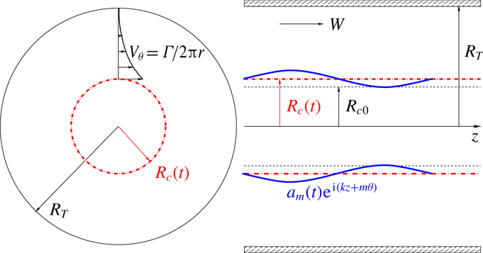
Sketch of a cylindrical bubble with surface modes in a vortex region.

We consider a bubble experiencing a dominant oscillation in the radial direction and a perturbation to surface modes as illustrated in figure 2. The compressibility of the external liquid flow is neglected considering the moderate variation of pressure in the present cases. The fluid compressibility was also proved to have little influence on the scattering of a multipole driven by a cavitated line vortex (Williams & O’Sher Reference Williams and O’Sher1970) or by a compact source (Yang, Feng & Leal Reference Yang, Feng and Leal1993). Therefore, the continuity equation reads
 $$\begin{eqnarray}\unicode[STIX]{x1D735}\boldsymbol{\cdot }\boldsymbol{u}=0,\end{eqnarray}$$
where
 $\boldsymbol{u}$
is the liquid velocity. The dominant radial velocity induced by the bubble dynamics is expressed as
 $R_{c}{\dot{R}}_{c}/r$
based on the requirement of mass conservation. The perturbed flow field induced by surface modes, described by means of velocity potential
 $\unicode[STIX]{x1D6F7}$
, can be solved according to the Laplace equation:
 $$\begin{eqnarray}\unicode[STIX]{x1D6FB}^{2}\unicode[STIX]{x1D6F7}=0.\end{eqnarray}$$
The velocity due to the dynamics of the bubble,
 $\boldsymbol{u}_{c}$
, is thus written as
 $$\begin{eqnarray}\boldsymbol{u}_{c}=\left(\frac{R_{c}{\dot{R}}_{c}}{r}+\unicode[STIX]{x1D700}\frac{\unicode[STIX]{x2202}\unicode[STIX]{x1D6F7}}{\unicode[STIX]{x2202}r}\right)\boldsymbol{e}_{r}+\unicode[STIX]{x1D700}\frac{1}{r}\frac{\unicode[STIX]{x2202}\unicode[STIX]{x1D6F7}}{\unicode[STIX]{x2202}\unicode[STIX]{x1D703}}\boldsymbol{e}_{\unicode[STIX]{x1D703}}+\unicode[STIX]{x1D700}\frac{\unicode[STIX]{x2202}\unicode[STIX]{x1D6F7}}{\unicode[STIX]{x2202}z}\boldsymbol{e}_{z}.\end{eqnarray}$$
The flow field induced by the free stream is superimposed on that induced by the bubble dynamics. Thus, the velocity in the liquid field can be expressed as
 $$\begin{eqnarray}\displaystyle \boldsymbol{u} & = & \displaystyle \boldsymbol{u}_{c}+\boldsymbol{U}=u_{r}\boldsymbol{e}_{r}+u_{\unicode[STIX]{x1D703}}\boldsymbol{e}_{\unicode[STIX]{x1D703}}+u_{z}\boldsymbol{e}_{z}\nonumber\\ \displaystyle & = & \displaystyle \left(\frac{R_{c}{\dot{R}}_{c}}{r}+\unicode[STIX]{x1D700}\frac{\unicode[STIX]{x2202}\unicode[STIX]{x1D6F7}}{\unicode[STIX]{x2202}r}\right)\boldsymbol{e}_{r}+\left(V_{\unicode[STIX]{x1D703}}+\unicode[STIX]{x1D700}\frac{1}{r}\frac{\unicode[STIX]{x2202}\unicode[STIX]{x1D6F7}}{\unicode[STIX]{x2202}\unicode[STIX]{x1D703}}\right)\boldsymbol{e}_{\unicode[STIX]{x1D703}}+\left(W+\unicode[STIX]{x1D700}\frac{\unicode[STIX]{x2202}\unicode[STIX]{x1D6F7}}{\unicode[STIX]{x2202}z}\right)\boldsymbol{e}_{z},\end{eqnarray}$$
where
 $u_{r}$
,
 $u_{\unicode[STIX]{x1D703}}$
and
 $u_{z}$
are the velocity components in cylindrical coordinates.
Next, we introduce the radial momentum equation:
 $$\begin{eqnarray}-\frac{1}{\unicode[STIX]{x1D70C}}\frac{\unicode[STIX]{x2202}p}{\unicode[STIX]{x2202}r}=\frac{\unicode[STIX]{x2202}u_{r}}{\unicode[STIX]{x2202}t}+\boldsymbol{u}\boldsymbol{\cdot }\unicode[STIX]{x1D735}u_{r}-\frac{u_{\unicode[STIX]{x1D703}}^{2}}{r},\end{eqnarray}$$
where
 $\unicode[STIX]{x1D70C}$
is the liquid density, while the viscosity is neglected. Gravity is neglected as well, which will be justified in § 3 with the given parameters. Substituting the velocity (2.10) and keeping the terms up to the order
 $O(\unicode[STIX]{x1D700})$
, we write out (2.11) as
 $$\begin{eqnarray}\displaystyle -\frac{1}{\unicode[STIX]{x1D70C}}\frac{\unicode[STIX]{x2202}p}{\unicode[STIX]{x2202}r} & = & \displaystyle ({\dot{R}}_{c}^{2}+R_{c}\ddot{R}_{c})\frac{1}{r}+\unicode[STIX]{x1D700}\frac{\unicode[STIX]{x2202}}{\unicode[STIX]{x2202}t}\left(\frac{\unicode[STIX]{x2202}\unicode[STIX]{x1D6F7}}{\unicode[STIX]{x2202}r}\right)\nonumber\\ \displaystyle & & \displaystyle -\,\frac{R_{c}^{2}{\dot{R}}_{c}^{2}}{r^{3}}+\unicode[STIX]{x1D700}\left(\frac{R_{c}{\dot{R}}_{c}}{r}\frac{\unicode[STIX]{x2202}^{2}\unicode[STIX]{x1D6F7}}{\unicode[STIX]{x2202}r^{2}}-\frac{R_{c}{\dot{R}}_{c}}{r^{2}}\frac{\unicode[STIX]{x2202}\unicode[STIX]{x1D6F7}}{\unicode[STIX]{x2202}r}+\frac{V_{\unicode[STIX]{x1D703}}}{r}\frac{\unicode[STIX]{x2202}^{2}\unicode[STIX]{x1D6F7}}{\unicode[STIX]{x2202}\unicode[STIX]{x1D703}\unicode[STIX]{x2202}r}+W\frac{\unicode[STIX]{x2202}^{2}\unicode[STIX]{x1D6F7}}{\unicode[STIX]{x2202}z\unicode[STIX]{x2202}r}\right)\nonumber\\ \displaystyle & & \displaystyle -\,\frac{V_{\unicode[STIX]{x1D703}}^{2}}{r}-\unicode[STIX]{x1D700}\frac{2V_{\unicode[STIX]{x1D703}}}{r^{2}}\frac{\unicode[STIX]{x2202}\unicode[STIX]{x1D6F7}}{\unicode[STIX]{x2202}\unicode[STIX]{x1D703}}.\end{eqnarray}$$
Integrating (2.12) from the bubble surface
 $r_{c}$
to the sidewall of the water tunnel
 $R_{T}$
leads to
 $$\begin{eqnarray}\displaystyle -\frac{1}{\unicode[STIX]{x1D70C}}(p_{T}-p_{c}) & = & \displaystyle \left.\left[({\dot{R}}_{c}^{2}+R_{c}\ddot{R}_{c})\ln r+\frac{R_{c}^{2}{\dot{R}}_{c}^{2}}{2r^{2}}+\unicode[STIX]{x1D700}\left(\frac{\unicode[STIX]{x2202}\unicode[STIX]{x1D6F7}}{\unicode[STIX]{x2202}t}+R_{c}{\dot{R}}_{c}\frac{1}{r}\frac{\unicode[STIX]{x2202}\unicode[STIX]{x1D6F7}}{\unicode[STIX]{x2202}r}+W\frac{\unicode[STIX]{x2202}\unicode[STIX]{x1D6F7}}{\unicode[STIX]{x2202}z}\right)\right]\right|_{r_{c}}^{R_{T}}\nonumber\\ \displaystyle & & \displaystyle -\int _{r_{c}}^{R_{T}}\frac{V_{\unicode[STIX]{x1D703}}^{2}}{r}\,\text{d}r+\unicode[STIX]{x1D700}\int _{r_{c}}^{R_{T}}\left(\frac{V_{\unicode[STIX]{x1D703}}}{r}\frac{\unicode[STIX]{x2202}^{2}\unicode[STIX]{x1D6F7}}{\unicode[STIX]{x2202}\unicode[STIX]{x1D703}\unicode[STIX]{x2202}r}-\frac{2V_{\unicode[STIX]{x1D703}}}{r^{2}}\frac{\unicode[STIX]{x2202}\unicode[STIX]{x1D6F7}}{\unicode[STIX]{x2202}\unicode[STIX]{x1D703}}\right)\text{d}r,\end{eqnarray}$$
where
 $p_{T}$
and
 $p_{c}$
are the pressure at the wall of the water tunnel and at the bubble interface, respectively. Owing to the confinement of the water tunnel, the logarithmic singularity for an infinite incompressible liquid is absent here. If we select the potential vortex model as a simple example, and assume the external flow of the cavitation bubble is in the potential region, the azimuthal velocity is given by
 $$\begin{eqnarray}V_{\unicode[STIX]{x1D703}}=\frac{\unicode[STIX]{x1D6E4}}{2\unicode[STIX]{x03C0}r},\end{eqnarray}$$
where
 $\unicode[STIX]{x1D6E4}$
is the circulation. Other vortex models can be applied, whereas the integration in (2.13) is difficult to express explicitly. Here, with potential vortex model (2.14), the integration is written out and (2.13) becomes
 $$\begin{eqnarray}\displaystyle -\frac{1}{\unicode[STIX]{x1D70C}}(p_{T}-p_{c}) & = & \displaystyle \left[({\dot{R}}_{c}^{2}+R_{c}\ddot{R}_{c})\ln r+\frac{R_{c}^{2}{\dot{R}}_{c}^{2}}{2r^{2}}+\frac{\unicode[STIX]{x1D6E4}^{2}}{8\unicode[STIX]{x03C0}^{2}r^{2}}\right.\nonumber\\ \displaystyle & & \displaystyle +\left.\!\left.\unicode[STIX]{x1D700}\left(\frac{\unicode[STIX]{x2202}\unicode[STIX]{x1D6F7}}{\unicode[STIX]{x2202}t}+R_{c}{\dot{R}}_{c}\frac{1}{r}\frac{\unicode[STIX]{x2202}\unicode[STIX]{x1D6F7}}{\unicode[STIX]{x2202}r}+\frac{\unicode[STIX]{x1D6E4}}{2\unicode[STIX]{x03C0}r^{2}}\frac{\unicode[STIX]{x2202}\unicode[STIX]{x1D6F7}}{\unicode[STIX]{x2202}\unicode[STIX]{x1D703}}+W\frac{\unicode[STIX]{x2202}\unicode[STIX]{x1D6F7}}{\unicode[STIX]{x2202}z}\right)\right]\right|_{r_{c}}^{R_{T}}\!.\end{eqnarray}$$
The continuity of velocity in the normal direction at the bubble interface yields the kinematic boundary condition
 $$\begin{eqnarray}\frac{\unicode[STIX]{x2202}S}{\unicode[STIX]{x2202}t}+\boldsymbol{u}\boldsymbol{\cdot }\unicode[STIX]{x1D735}S=0,\end{eqnarray}$$
where the surface function
 $S$
has been defined in (2.2). The stress balance at the interface between the pressure jump and the surface tension provides the dynamic boundary condition
 $$\begin{eqnarray}-p_{c}=-p_{v}-p_{g}+\unicode[STIX]{x1D70E}\unicode[STIX]{x1D735}\boldsymbol{\cdot }\boldsymbol{n},\end{eqnarray}$$
where
 $p_{v}$
is the saturated vapour pressure and
 $p_{g}$
is the partial pressure of gas, which changes according to a polytropic law
 $$\begin{eqnarray}p_{g}=p_{g0}\left(\frac{V_{c0}}{V_{c}}\right)^{\unicode[STIX]{x1D701}}\!,\end{eqnarray}$$
where
 $p_{g0}$
is the gas pressure at the initial moment and
 $\unicode[STIX]{x1D701}$
is the polytropic index.
2.3 Dynamic equations without confinement
In view of the surface shape function (2.2), we suppose that the normal-mode solution to the Laplace equation (2.8) in cylindrical coordinates has the form
 $$\begin{eqnarray}\unicode[STIX]{x1D6F7}(r,\unicode[STIX]{x1D703},z;t)=\unicode[STIX]{x1D719}(r,t)\text{e}^{\text{i}(kz+m\unicode[STIX]{x1D703})}.\end{eqnarray}$$
Substituting (2.19) into (2.8), we obtain
 $$\begin{eqnarray}\frac{\unicode[STIX]{x2202}^{2}\unicode[STIX]{x1D719}}{\unicode[STIX]{x2202}r^{2}}+\frac{\unicode[STIX]{x2202}\unicode[STIX]{x1D719}}{r\unicode[STIX]{x2202}r}+\left(-k^{2}-\frac{m^{2}}{r^{2}}\right)\unicode[STIX]{x1D719}=0.\end{eqnarray}$$
The general solution to (2.20) is the sum of Hankel functions of the first and second kinds:
 $$\begin{eqnarray}\unicode[STIX]{x1D719}(r,t)=A_{m}(t)\text{H}_{m}^{1}(\text{i}kr)+B_{m}(t)\text{H}_{m}^{2}(\text{i}kr),\end{eqnarray}$$
where
 $A_{m}(t)$
and
 $B_{m}(t)$
are unknowns to be determined. In this section, we only consider the radiation wave and neglect the reflection from the tunnel wall temporarily. Therefore, the Hankel function of the second kind is discarded. The effect of confinement will be discussed in § 2.4. Here the velocity potential is expressed as
 $$\begin{eqnarray}\unicode[STIX]{x1D6F7}(r,\unicode[STIX]{x1D703},z;t)=A_{m}(t)\text{H}_{m}^{1}(\text{i}kr)\text{e}^{\text{i}(kz+m\unicode[STIX]{x1D703})}.\end{eqnarray}$$
Combining the kinematic boundary condition (2.16), the surface function (2.2) and the total velocity
 $\boldsymbol{u}$
(2.10), we obtain the coefficients
 $A_{m}$
(see appendix A):
 $$\begin{eqnarray}A_{m}=\frac{1}{\text{H}_{m}^{1\prime }(\text{i}kR_{c})}\left[{\dot{a}}_{m}+a_{m}\frac{{\dot{R}}_{c}}{R_{c}}+\text{i}a_{m}\left(\frac{mV_{\unicode[STIX]{x1D703}c}}{R_{c}}+kW\right)\right],\end{eqnarray}$$
where
 $V_{\unicode[STIX]{x1D703}c}$
is the azimuthal velocity at the bubble interface. For the potential vortex,
 $V_{\unicode[STIX]{x1D703}c}=\unicode[STIX]{x1D6E4}/(2\unicode[STIX]{x03C0}R_{c})$
. In the above,
 $\text{H}_{m}^{1\prime }(\text{i}kR_{c})$
is the derivative of the Hankel function with respect to
 $r$
and evaluated at
 $r=R_{c}$
, i.e.
 $\text{H}_{m}^{1\prime }(\text{i}kR_{c})=\unicode[STIX]{x2202}\text{H}_{m}^{1}(\text{i}kr)/\unicode[STIX]{x2202}r|_{r=R_{c}}$
.
Substituting the velocity potential
 $\unicode[STIX]{x1D6F7}$
(2.22) along with coefficient
 $A_{m}$
(2.23) into (2.15) and combining the dynamic boundary condition (2.17), we obtain the dynamic equation at the order
 $O(\unicode[STIX]{x1D700}^{0})$
,
 $$\begin{eqnarray}\displaystyle & & \displaystyle (R_{c}\ddot{R}_{c}+{\dot{R}}_{c}^{2})\ln \left(\frac{R_{T}}{R_{c}}\right)+\frac{R_{c}^{2}{\dot{R}}_{c}^{2}}{2}\left(\frac{1}{R_{T}^{2}}-\frac{1}{R_{c}^{2}}\right)\nonumber\\ \displaystyle & & \displaystyle \quad =\frac{1}{\unicode[STIX]{x1D70C}}\left[p_{v}+p_{g0}\left(\frac{R_{c0}}{R_{c}}\right)^{2\unicode[STIX]{x1D701}}-\frac{\unicode[STIX]{x1D70E}}{R_{c}}-p_{T}\right]+\frac{\unicode[STIX]{x1D6E4}^{2}}{8\unicode[STIX]{x03C0}^{2}}\left(\frac{1}{R_{c}^{2}}-\frac{1}{R_{T}^{2}}\right),\end{eqnarray}$$
and the dynamic equation at the order
 $O(\unicode[STIX]{x1D700}^{1})$
,
 $$\begin{eqnarray}\displaystyle & & \displaystyle \!\!\ddot{a}_{m}+\left[\frac{{\dot{R}}_{c}}{R_{c}}+\frac{\text{H}_{m}^{1\prime }(\text{i}kR_{c})}{\text{H}_{m}^{1}(\text{i}kR_{c})}{\dot{R}}_{c}+\text{i}\left(2kW+\frac{m\unicode[STIX]{x1D6E4}}{\unicode[STIX]{x03C0}R_{c}^{2}}\right)\right]{\dot{a}}_{m}\nonumber\\ \displaystyle & & \displaystyle \!\!\quad +\left[\vphantom{\left(\frac{m\unicode[STIX]{x1D6E4}}{R_{c}^{2}}\right)^{2}}\frac{\ddot{R}_{c}}{R_{c}}-\frac{{\dot{R}}_{c}^{2}}{R_{c}^{2}}+\text{i}kW\frac{{\dot{R}}_{c}}{R_{c}}-\text{i}\frac{m\unicode[STIX]{x1D6E4}{\dot{R}}_{c}}{2\unicode[STIX]{x03C0}R_{c}^{3}}-\frac{\text{H}_{m}^{1\prime }(\text{i}kR_{c})}{\text{H}_{m}^{1}(\text{i}kR_{c})}\left(-\frac{{\dot{R}}_{c}^{2}}{R_{c}}-\ddot{R}_{c}-\text{i}\frac{m\unicode[STIX]{x1D6E4}}{2\unicode[STIX]{x03C0}R_{c}^{2}}{\dot{R}}_{c}-\text{i}kW{\dot{R}}_{c}\right)\right.\quad \nonumber\\ \displaystyle & & \displaystyle \!\!\quad -\left.\frac{\text{H}_{m}^{1\prime }(\text{i}kR_{c})}{\text{H}_{m}^{1}(\text{i}kR_{c})}\left(\frac{\unicode[STIX]{x1D6E4}^{2}}{4\unicode[STIX]{x03C0}^{2}R_{c}^{3}}+\frac{\unicode[STIX]{x1D70E}}{\unicode[STIX]{x1D70C}R_{c}^{2}}(m^{2}+k^{2}R_{c}^{2}-1)\right)-\left(kW+\frac{m\unicode[STIX]{x1D6E4}}{2\unicode[STIX]{x03C0}R_{c}^{2}}\right)^{2}\right]a_{m}=0.\qquad\end{eqnarray}$$
The Rayleigh–Plesset like equation (2.24) describes the nonlinear dynamics in the radial direction. This equation is consistent with the work of Chahine (Reference Chahine1995) except that the tangential velocity is given according to the potential vortex model here. Supposing
 $R_{c}(t)=R_{c0}[1+\bar{\unicode[STIX]{x1D700}}x(t)]$
, where
 $\bar{\unicode[STIX]{x1D700}}\ll 1$
, and linearizing (2.24), we obtain a linear oscillatory equation and then the natural frequency of the radial mode,
 $\unicode[STIX]{x1D714}_{R}$
, as
 $$\begin{eqnarray}\unicode[STIX]{x1D714}_{R}^{2}=\left.\left(\frac{2\unicode[STIX]{x1D701}p_{g0}}{\unicode[STIX]{x1D70C}R_{c0}^{2}}-\frac{\unicode[STIX]{x1D70E}}{\unicode[STIX]{x1D70C}R_{c0}^{3}}+\frac{\unicode[STIX]{x1D6E4}^{2}}{4\unicode[STIX]{x03C0}^{2}R_{c0}^{4}}\right)\right/\!\ln \left(\frac{R_{T}}{R_{c0}}\right).\end{eqnarray}$$
This formula is consistent with the work of Choi et al. (Reference Choi, Hsiao, Chahine and Ceccio2009) if the surface tension and the partial pressure of the gas are neglected. Equation (2.25) is the linear dynamic equation for the
 $m$
th-order surface mode. Supposing
 $a_{m}$
has the form
 $a_{m}\sim \text{e}^{-\text{i}\unicode[STIX]{x1D714}_{m}t}$
and substituting it into (2.25), we obtain the characteristic equation and then the natural frequency of surface mode,
 $\unicode[STIX]{x1D714}_{m}$
, as
 $$\begin{eqnarray}\displaystyle \unicode[STIX]{x1D714}_{m\pm }=kW+\frac{m\unicode[STIX]{x1D6E4}}{2\unicode[STIX]{x03C0}R_{c0}^{2}}\pm \sqrt{-\frac{\text{H}_{m}^{1\prime }(\text{i}kR_{c0})}{\text{H}_{m}^{1}(\text{i}kR_{c0})}\left[\frac{\unicode[STIX]{x1D6E4}^{2}}{4\unicode[STIX]{x03C0}^{2}R_{c0}^{3}}+\frac{\unicode[STIX]{x1D70E}}{\unicode[STIX]{x1D70C}R_{c0}^{2}}(m^{2}+k^{2}R_{c0}^{2}-1)\right]}, & & \displaystyle\end{eqnarray}$$
which is consistent with the dispersion relation obtained by Pennings et al. (Reference Pennings, Bosschers, Westerweel and van Terwisga2015). The
 $\pm$
sign represents retrograde or co-grade rotation of the angular velocity at the interface relative to the external flow field, which also exists in the dispersion relation for a vortex without cavitation (Saffman Reference Saffman1992). While deriving the natural frequency of the surface mode (2.27), we temporarily decouple the surface mode from the radial mode by neglecting the radial variation, i.e. assuming
 $R_{c}=R_{c0}$
,
 ${\dot{R}}_{c}=0$
and
 $\ddot{R}_{c}=0$
in the dynamic equation (2.25).
2.4 Dynamic equations with confinement
In the previous section, the reflective wave from confinements was discarded for the surface modes. Next, we will incorporate the influence of the sidewall and derive the dynamic equation of the surface mode for a cylindrical cavitation bubble in a water tunnel. The governing equations are the same as those in § 2.2 and the solution is similar to § 2.3 except that the Hankel function of the second kind in (2.21) cannot be neglected, since it is associated with the reflected flow from the tunnel wall. To determine the coefficients
 $A_{m}$
and
 $B_{m}$
, an additional boundary condition must be imposed. Considering that the volume change due to the surface mode is of higher order, as given in (2.5), we regard the normal velocity at the tunnel wall induced by the surface modes as zero, i.e.
 $$\begin{eqnarray}\left.\frac{\unicode[STIX]{x2202}\unicode[STIX]{x1D6F7}}{\unicode[STIX]{x2202}r}\right|_{r=R_{T}}=0.\end{eqnarray}$$
Combining this condition at the tunnel wall and the kinematic boundary condition at the bubble surface (2.16), we obtain the coefficients
 $A_{m}$
and
 $B_{m}$
(see appendix A) as
 $$\begin{eqnarray}\displaystyle & \displaystyle A_{m}=\frac{1}{\unicode[STIX]{x1D6FC}}\left[{\dot{a}}_{m}+a_{m}\frac{{\dot{R}}_{c}}{R_{c}}+\text{i}a_{m}\left(\frac{mV_{\unicode[STIX]{x1D703}c}}{R_{c}}+kW\right)\right], & \displaystyle\end{eqnarray}$$
 $$\begin{eqnarray}\displaystyle & \displaystyle B_{m}=\frac{1}{\unicode[STIX]{x1D6FD}}\left[{\dot{a}}_{m}+a_{m}\frac{{\dot{R}}_{c}}{R_{c}}+\text{i}a_{m}\left(\frac{mV_{\unicode[STIX]{x1D703}c}}{R_{c}}+kW\right)\right], & \displaystyle\end{eqnarray}$$
where
 $$\begin{eqnarray}\displaystyle & \displaystyle \unicode[STIX]{x1D6FC}=\text{H}_{m}^{1\prime }(\text{i}kR_{c})-\text{H}_{m}^{2\prime }(\text{i}kR_{c})\frac{\text{H}_{m}^{1\prime }(\text{i}kR_{T})}{\text{H}_{m}^{2\prime }(\text{i}kR_{T})}, & \displaystyle\end{eqnarray}$$
 $$\begin{eqnarray}\displaystyle & \displaystyle \unicode[STIX]{x1D6FD}=\text{H}_{m}^{2\prime }(\text{i}kR_{c})-\text{H}_{m}^{1\prime }(\text{i}kR_{c})\frac{\text{H}_{m}^{2\prime }(\text{i}kR_{T})}{\text{H}_{m}^{1\prime }(\text{i}kR_{T})}. & \displaystyle\end{eqnarray}$$
Following the same procedure of collecting the radial momentum equation as in § 2.3, whose details are also given in appendix B, we obtain the dynamic equation for the
 $m$
th-order surface mode in a confinement as follows:
 $$\begin{eqnarray}\displaystyle & & \displaystyle \ddot{a}_{m}+\left[\frac{{\dot{R}}_{c}}{R_{c}}+\frac{\unicode[STIX]{x1D6FF}_{1}}{\unicode[STIX]{x1D706}}{\dot{R}}_{c}-\frac{\unicode[STIX]{x1D6FF}_{2}}{\unicode[STIX]{x1D706}}\frac{R_{c}}{R_{T}}{\dot{R}}_{c}+\text{i}\left(2kW+\frac{2\unicode[STIX]{x1D706}+\unicode[STIX]{x1D6FE}}{\unicode[STIX]{x1D706}}\frac{m\unicode[STIX]{x1D6E4}}{2\unicode[STIX]{x03C0}R_{c}^{2}}-\frac{\unicode[STIX]{x1D6FE}}{\unicode[STIX]{x1D706}}\frac{m\unicode[STIX]{x1D6E4}}{2\unicode[STIX]{x03C0}R_{T}^{2}}\right)\right]{\dot{a}}_{m}\nonumber\\ \displaystyle & & \displaystyle \quad +\left\{\vphantom{\left(\frac{m\unicode[STIX]{x1D6E4}}{R_{T}^{2}}\right)^{2}}\frac{\ddot{R}_{c}}{R_{c}}-\frac{{\dot{R}}_{c}^{2}}{R_{c}^{2}}-\text{i}\frac{m\unicode[STIX]{x1D6E4}{\dot{R}}_{c}}{2\unicode[STIX]{x03C0}R_{c}^{3}}+\frac{\unicode[STIX]{x1D6FF}_{1}}{\unicode[STIX]{x1D706}}\frac{{\dot{R}}_{c}^{2}}{R_{c}}-\frac{\unicode[STIX]{x1D6FF}_{2}}{\unicode[STIX]{x1D706}}\frac{R_{c}}{R_{T}}\frac{{\dot{R}}_{c}^{2}}{R_{c}}+\frac{\unicode[STIX]{x1D6FC}\unicode[STIX]{x1D6FD}}{\unicode[STIX]{x1D706}}\ddot{R}_{c}\right.\nonumber\\ \displaystyle & & \displaystyle \quad +\,\,\text{i}\frac{m\unicode[STIX]{x1D6E4}}{2\unicode[STIX]{x03C0}}\left(-\frac{\unicode[STIX]{x1D6FE}}{\unicode[STIX]{x1D706}R_{T}^{2}R_{c}}+\frac{\unicode[STIX]{x1D6FE}}{\unicode[STIX]{x1D706}R_{c}^{3}}+\frac{\unicode[STIX]{x1D6FF}_{1}}{\unicode[STIX]{x1D706}R_{c}^{2}}-\frac{\unicode[STIX]{x1D6FF}_{2}}{\unicode[STIX]{x1D706}}\frac{1}{R_{T}R_{c}}\right){\dot{R}}_{c}\nonumber\\ \displaystyle & & \displaystyle \quad +\,\,\text{i}\left(\frac{1}{R_{c}}+\frac{\unicode[STIX]{x1D6FF}_{1}}{\unicode[STIX]{x1D706}}-\frac{\unicode[STIX]{x1D6FF}_{2}}{\unicode[STIX]{x1D706}}\frac{R_{c}}{R_{T}}\right)kW{\dot{R}}_{c}-\frac{\unicode[STIX]{x1D6FC}\unicode[STIX]{x1D6FD}}{\unicode[STIX]{x1D706}}\frac{\unicode[STIX]{x1D6E4}^{2}}{4\unicode[STIX]{x03C0}^{2}R_{c}^{3}}-\frac{\unicode[STIX]{x1D6FC}\unicode[STIX]{x1D6FD}}{\unicode[STIX]{x1D706}}\frac{\unicode[STIX]{x1D70E}}{\unicode[STIX]{x1D70C}R_{c}^{2}}(m^{2}+k^{2}R_{c}^{2}-1)\nonumber\\ \displaystyle & & \displaystyle \quad +\left.\!\left[\frac{\unicode[STIX]{x1D6FE}}{\unicode[STIX]{x1D706}}\frac{m\unicode[STIX]{x1D6E4}}{4\unicode[STIX]{x03C0}}\left(\frac{1}{R_{T}^{2}}-\frac{1}{R_{c}^{2}}\right)\right]^{2}-\left(kW+\frac{2\unicode[STIX]{x1D706}+\unicode[STIX]{x1D6FE}}{\unicode[STIX]{x1D706}}\frac{m\unicode[STIX]{x1D6E4}}{4\unicode[STIX]{x03C0}R_{c}^{2}}-\frac{\unicode[STIX]{x1D6FE}}{\unicode[STIX]{x1D706}}\frac{m\unicode[STIX]{x1D6E4}}{4\unicode[STIX]{x03C0}R_{T}^{2}}\right)^{2}\right\}a_{m}=0,\qquad \quad\end{eqnarray}$$
where
 $$\begin{eqnarray}\displaystyle & \displaystyle \unicode[STIX]{x1D706}=[\text{H}_{m}^{2}(\text{i}kR_{c})-\text{H}_{m}^{2}(\text{i}kR_{T})]\unicode[STIX]{x1D6FC}+[\text{H}_{m}^{1}(\text{i}kR_{c})-\text{H}_{m}^{1}(\text{i}kR_{T})]\unicode[STIX]{x1D6FD}, & \displaystyle\end{eqnarray}$$
 $$\begin{eqnarray}\displaystyle & \displaystyle \unicode[STIX]{x1D6FE}=\text{H}_{m}^{2}(\text{i}kR_{T})\unicode[STIX]{x1D6FC}+\text{H}_{m}^{1}(\text{i}kR_{T})\unicode[STIX]{x1D6FD}, & \displaystyle\end{eqnarray}$$
 $$\begin{eqnarray}\displaystyle & \displaystyle \unicode[STIX]{x1D6FF}_{1}=\text{H}_{m}^{2\prime }(\text{i}kR_{c})\unicode[STIX]{x1D6FC}+\text{H}_{m}^{1\prime }(\text{i}kR_{c})\unicode[STIX]{x1D6FD}, & \displaystyle\end{eqnarray}$$
 $$\begin{eqnarray}\displaystyle & \displaystyle \unicode[STIX]{x1D6FF}_{2}=\text{H}_{m}^{2\prime }(\text{i}kR_{T})\unicode[STIX]{x1D6FC}+\text{H}_{m}^{1\prime }(\text{i}kR_{T})\unicode[STIX]{x1D6FD}. & \displaystyle\end{eqnarray}$$
In a similar way to that in the previous section, we decouple the surface mode from the radial mode, suppose
 $a_{m}$
has the form
 $a_{m}\sim \text{e}^{-\text{i}\unicode[STIX]{x1D714}_{m}t}$
, substitute it into (2.33), and obtain the dispersion relation:
 $$\begin{eqnarray}\displaystyle \bar{\unicode[STIX]{x1D714}}_{m\pm } & = & \displaystyle kW-\frac{m\unicode[STIX]{x1D6E4}}{4\unicode[STIX]{x03C0}\unicode[STIX]{x1D706}}\left(\frac{\unicode[STIX]{x1D6FE}}{R_{T}^{2}}-\frac{2\unicode[STIX]{x1D706}+\unicode[STIX]{x1D6FE}}{R_{c0}^{2}}\right)\nonumber\\ \displaystyle & & \displaystyle \pm \,\sqrt{-\frac{\unicode[STIX]{x1D6FC}\unicode[STIX]{x1D6FD}}{\unicode[STIX]{x1D706}}\frac{\unicode[STIX]{x1D6E4}^{2}}{4\unicode[STIX]{x03C0}^{2}R_{c0}^{3}}-\frac{\unicode[STIX]{x1D6FC}\unicode[STIX]{x1D6FD}}{\unicode[STIX]{x1D706}}\frac{\unicode[STIX]{x1D70E}}{\unicode[STIX]{x1D70C}R_{c0}^{2}}(m^{2}+k^{2}R_{c0}^{2}-1)+\left[\frac{\unicode[STIX]{x1D6FE}}{\unicode[STIX]{x1D706}}\frac{m\unicode[STIX]{x1D6E4}}{4\unicode[STIX]{x03C0}}\left(\frac{1}{R_{T}^{2}}-\frac{1}{R_{c0}^{2}}\right)\right]^{2}}.\nonumber\\ \displaystyle & & \displaystyle\end{eqnarray}$$
Since all surface modes conserve volume at the order
 $O(\unicode[STIX]{x1D700}^{2})$
according to (2.5), they can oscillate freely following (2.33) without logarithmic singularity even when the flow domain is presumed infinite in extent, i.e.
 $R_{T}\rightarrow \infty$
, the same conclusion as obtained by Ilinskii et al. (Reference Ilinskii, Zabolotskaya, Hay and Hamilton2012) for a cylindrical bubble in a narrow channel. Numerical analysis on the effects of confinements will be shown in § 3.2.
2.5 Dynamic equations with viscous stress
Next we consider the viscous effect at the interface. Including the viscous stress, the dynamic boundary condition at the interface (2.17) becomes
 $$\begin{eqnarray}-p_{c}+2\unicode[STIX]{x1D707}\boldsymbol{n}\boldsymbol{\cdot }\unicode[STIX]{x1D640}\boldsymbol{\cdot }\boldsymbol{n}=-p_{v}-p_{g}+\unicode[STIX]{x1D70E}\unicode[STIX]{x1D735}\boldsymbol{\cdot }\boldsymbol{n},\end{eqnarray}$$
where
 $\unicode[STIX]{x1D707}$
is the liquid viscosity while the viscosities of gas and vapour are neglected; and
 $\unicode[STIX]{x1D640}=(\unicode[STIX]{x1D735}\boldsymbol{u}+\unicode[STIX]{x1D735}\boldsymbol{u}^{\text{T}})/2$
is the strain-rate tensor. The explicit expression of
 $\boldsymbol{n}\boldsymbol{\cdot }\unicode[STIX]{x1D640}\boldsymbol{\cdot }\boldsymbol{n}$
is derived in appendix C. Accordingly, the dynamic equations of the radial and surface modes become
 $$\begin{eqnarray}\displaystyle & & \displaystyle (R_{c}\ddot{R}_{c}+{\dot{R}}_{c}^{2})\ln \left(\frac{R_{T}}{R_{c}}\right)+\frac{R_{c}^{2}{\dot{R}}_{c}^{2}}{2}\left(\frac{1}{R_{T}^{2}}-\frac{1}{R_{c}^{2}}\right)\nonumber\\ \displaystyle & & \displaystyle \quad =\frac{1}{\unicode[STIX]{x1D70C}}\left[p_{v}+p_{g0}\left(\frac{R_{c0}}{R_{c}}\right)^{2\unicode[STIX]{x1D701}}-\frac{2\unicode[STIX]{x1D707}{\dot{R}}_{c}}{R_{c}}-\frac{\unicode[STIX]{x1D70E}}{R_{c}}-p_{T}\right]+\frac{\unicode[STIX]{x1D6E4}^{2}}{8\unicode[STIX]{x03C0}^{2}}\left(\frac{1}{R_{c}^{2}}-\frac{1}{R_{T}^{2}}\right),\end{eqnarray}$$
and
 $$\begin{eqnarray}\displaystyle & & \displaystyle \!\!\ddot{a}_{m}+\left[\frac{{\dot{R}}_{c}}{R_{c}}+\frac{\text{H}_{m}^{1\prime }(\text{i}kR_{c})}{\text{H}_{m}^{1}(\text{i}kR_{c})}{\dot{R}}_{c}+\frac{\text{H}_{m}^{1\prime \prime }(\text{i}kR_{c})}{\text{H}_{m}^{1}(\text{i}kR_{c})}\frac{2\unicode[STIX]{x1D707}}{\unicode[STIX]{x1D70C}}+\text{i}\left(2kW+\frac{m\unicode[STIX]{x1D6E4}}{\unicode[STIX]{x03C0}R_{c}^{2}}\right)\right]{\dot{a}}_{m}\nonumber\\ \displaystyle & & \displaystyle \qquad \!\!+\left[\vphantom{\left(\frac{m\unicode[STIX]{x1D6E4}}{R_{T}^{2}}\right)^{2}}\frac{\ddot{R}_{c}}{R_{c}}-\frac{{\dot{R}}_{c}^{2}}{R_{c}^{2}}+\text{i}kW\frac{{\dot{R}}_{c}}{R_{c}}-\text{i}\frac{m\unicode[STIX]{x1D6E4}{\dot{R}}_{c}}{2\unicode[STIX]{x03C0}R_{c}^{3}}-\frac{\text{H}_{m}^{1\prime }(\text{i}kR_{c})}{\text{H}_{m}^{1}(\text{i}kR_{c})}\right.\nonumber\\ \displaystyle & & \displaystyle \qquad \!\!\times \left(-\frac{{\dot{R}}_{c}^{2}}{R_{c}}-\ddot{R}_{c}-\frac{4\unicode[STIX]{x1D707}{\dot{R}}_{c}}{\unicode[STIX]{x1D70C}R_{c}^{2}}-\text{i}\frac{m\unicode[STIX]{x1D6E4}}{2\unicode[STIX]{x03C0}R_{c}^{2}}{\dot{R}}_{c}-\text{i}kW{\dot{R}}_{c}\right)\nonumber\\ \displaystyle & & \displaystyle \qquad \!\!+\,\frac{\text{H}_{m}^{1\prime \prime }(\text{i}kR_{c})}{\text{H}_{m}^{1}(\text{i}kR_{c})}\frac{\unicode[STIX]{x1D707}}{\unicode[STIX]{x1D70C}}\left(\frac{2{\dot{R}}_{c}}{R_{c}}+\text{i}\frac{m\unicode[STIX]{x1D6E4}}{\unicode[STIX]{x03C0}R_{c}^{2}}+2\text{i}kW\right)\nonumber\\ \displaystyle & & \displaystyle \qquad \!\!-\left.\frac{\text{H}_{m}^{1\prime }(\text{i}kR_{c})}{\text{H}_{m}^{1}(\text{i}kR_{c})}\left(\frac{\unicode[STIX]{x1D6E4}^{2}}{4\unicode[STIX]{x03C0}^{2}R_{c}^{3}}+\frac{\unicode[STIX]{x1D70E}}{\unicode[STIX]{x1D70C}R_{c}^{2}}(m^{2}+k^{2}R_{c}^{2}-1)-\text{i}\frac{2m\unicode[STIX]{x1D707}\unicode[STIX]{x1D6E4}}{\unicode[STIX]{x03C0}\unicode[STIX]{x1D70C}R_{c}^{3}}\right)-\left(kW+\frac{m\unicode[STIX]{x1D6E4}}{2\unicode[STIX]{x03C0}R_{c}^{2}}\right)^{2}\right]a_{m}\nonumber\\ \displaystyle & & \displaystyle \!\!\quad =0.\end{eqnarray}$$
Without the viscous terms, these two equations reduce to (2.24) and (2.25).
Besides supposing
 $R_{c}(t)=R_{c0}[1+\bar{\unicode[STIX]{x1D700}}x(t)]$
to linearize (2.40), as we have done in § 2.3, here we further suppose that
 $x(t)=\text{e}^{-\unicode[STIX]{x1D712}_{R}t}$
, so that the characteristic equation of (2.40) is obtained:
 $$\begin{eqnarray}\ln \left(\frac{R_{T}}{R_{c0}}\right)R_{c0}^{2}\unicode[STIX]{x1D712}_{R}^{2}+\frac{2\unicode[STIX]{x1D707}}{\unicode[STIX]{x1D70C}}\unicode[STIX]{x1D712}_{R}+\frac{2\unicode[STIX]{x1D701}p_{g0}}{\unicode[STIX]{x1D70C}}-\frac{\unicode[STIX]{x1D70E}}{\unicode[STIX]{x1D70C}R_{c0}}+\frac{\unicode[STIX]{x1D6E4}^{2}}{4\unicode[STIX]{x03C0}^{2}R_{c0}^{2}}=0,\end{eqnarray}$$
whose solution is
 $$\begin{eqnarray}\unicode[STIX]{x1D712}_{R}=\frac{\unicode[STIX]{x1D707}}{\unicode[STIX]{x1D70C}R_{c0}^{2}\ln \left({\displaystyle \frac{R_{T}}{R_{c0}}}\right)}\pm \frac{1}{\ln \left({\displaystyle \frac{R_{T}}{R_{c0}}}\right)}\sqrt{\frac{\unicode[STIX]{x1D707}^{2}}{\unicode[STIX]{x1D70C}^{2}R_{c0}^{4}}-\ln \left(\frac{R_{T}}{R_{c0}}\right)\left(\frac{2\unicode[STIX]{x1D701}p_{g0}}{\unicode[STIX]{x1D70C}R_{c0}^{2}}-\frac{\unicode[STIX]{x1D70E}}{\unicode[STIX]{x1D70C}R_{c0}^{3}}+\frac{\unicode[STIX]{x1D6E4}^{2}}{4\unicode[STIX]{x03C0}^{2}R_{c0}^{4}}\right)}.\end{eqnarray}$$
Note that
 $\unicode[STIX]{x1D712}_{R}$
is a complex number, whose imaginary part represents the natural frequency. If neglecting the viscous term, its imaginary part is consistent with (2.26). The real part of
 $\unicode[STIX]{x1D712}_{R}$
represents the growth or damping of the oscillatory amplitude, which will be discussed in 3.3.
Similarly, we suppose that
 $a_{m}(t)=\text{e}^{-\unicode[STIX]{x1D712}_{m}t}$
, where
 $\unicode[STIX]{x1D712}_{m}$
is also a complex number. Substituting it into (2.41) yields its characteristic equation and then the eigenvalue:
 $$\begin{eqnarray}\displaystyle \unicode[STIX]{x1D712}_{m} & = & \displaystyle \frac{\text{H}_{m}^{1\prime \prime }(\text{i}kR_{c0})}{\text{H}_{m}^{1}(\text{i}kR_{c0})}\frac{\unicode[STIX]{x1D707}}{\unicode[STIX]{x1D70C}}+\text{i}\left(kW+\frac{m\unicode[STIX]{x1D6E4}}{2\unicode[STIX]{x03C0}R_{c0}^{2}}\right)\nonumber\\ \displaystyle & & \displaystyle \pm \,\sqrt{\frac{\text{H}_{m}^{1\prime }(\text{i}kR_{c0})}{\text{H}_{m}^{1}(\text{i}kR_{c0})}\left[\frac{\unicode[STIX]{x1D6E4}^{2}}{4\unicode[STIX]{x03C0}^{2}R_{c0}^{3}}+\frac{\unicode[STIX]{x1D70E}}{\unicode[STIX]{x1D70C}R_{c0}^{2}}(m^{2}+k^{2}R_{c0}^{2}-1)-\text{i}\frac{2m\unicode[STIX]{x1D707}\unicode[STIX]{x1D6E4}}{\unicode[STIX]{x03C0}\unicode[STIX]{x1D70C}R_{c0}^{3}}\right]+\left(\frac{\text{H}_{m}^{1\prime \prime }(\text{i}kR_{c0})}{\text{H}_{m}^{1}(\text{i}kR_{c0})}\frac{\unicode[STIX]{x1D707}}{\unicode[STIX]{x1D70C}}\right)^{\!2}}\!.\nonumber\\ \displaystyle & & \displaystyle\end{eqnarray}$$
The imaginary part of (2.44), if the viscous terms are neglected, reduces to the dispersion relation (2.27).
3 Results and discussion
In this section, we will solve the equation system formulated in §§ 2.3, 2.4 and 2.5. At the initial moment, the bubble is assumed to be stationary in §§ 3.1–3.5, i.e.
 ${\dot{R}}_{c0}=0$
and
 $\ddot{R}_{c0}=0$
, and an initial radial velocity is prescribed in § 3.6. A small disturbance is applied to the surface mode, given by
 $a_{m}(t=0)/R_{c0}=0.01$
. We employ the fourth-order Runge–Kutta method to solve the dynamic equations of radial mode (2.24) (or (2.40)) and surface mode (2.25) (or (2.33), (2.41)). The parameters are selected according to the typical values in Pennings et al. (Reference Pennings, Bosschers, Westerweel and van Terwisga2015). We consider a cylindrical cavitation bubble with initial radius
 $R_{c0}=2.3$
mm, unless specified otherwise, suspended in water with density
 $\unicode[STIX]{x1D70C}=1000~\text{kg}~\text{m}^{-3}$
, viscosity
 $\unicode[STIX]{x1D707}=0.001~\text{kg}~\text{m}^{-1}~\text{s}^{-1}$
and surface tension
 $\unicode[STIX]{x1D70E}=0.0729~\text{N}~\text{m}^{-1}$
, and confined in a water tunnel with radius
 $R_{T}=0.3$
m. The saturated vapour pressure takes the value
 $p_{v}=2300$
Pa. The free-stream velocity is given by
 $W=6.3~\text{m}~\text{s}^{-1}$
. Considering a potential vortex, we have a circulation
 $\unicode[STIX]{x1D6E4}=0.066~\text{m}^{2}~\text{s}^{-1}$
associated with the azimuthal velocity at the bubble interface
 $V_{\unicode[STIX]{x1D703}c}=4.6~\text{m}~\text{s}^{-1}$
. The wavenumber
 $k$
is assigned within the range in the experimental observation. In fact, it is related to the stability in the axial direction (Fabre, Sipp & Jacquin Reference Fabre, Sipp and Jacquin2006), while we do not consider it in our model. We focus on the modes
 $m=0$
and
 $m=2$
, since these two modes were observed most frequently in experiments (Arndt et al.
Reference Arndt, Arakeri and Higuchi1991). The limited appearance of higher-order surface modes may be attributed to the substantial damping of the vortex with large azimuthal wavenumber (Fabre et al.
Reference Fabre, Sipp and Jacquin2006). The cavitation number
 $\unicode[STIX]{x1D70E}_{v}$
and the pressure at the tunnel wall
 $p_{T}$
are calculated according to the Bernoulli integration for the potential vortex flow (Pennings et al.
Reference Pennings, Bosschers, Westerweel and van Terwisga2015),
 $$\begin{eqnarray}\frac{V_{\unicode[STIX]{x1D703}c}}{W}=\sqrt{\frac{2(p_{T}-p_{v})}{\unicode[STIX]{x1D70C}W^{2}}}=\sqrt{\unicode[STIX]{x1D70E}_{v}},\end{eqnarray}$$
to be
 $\unicode[STIX]{x1D70E}_{v}=0.53$
and
 $p_{T}=12\,817$
Pa.
3.1 Effects of gas pressure
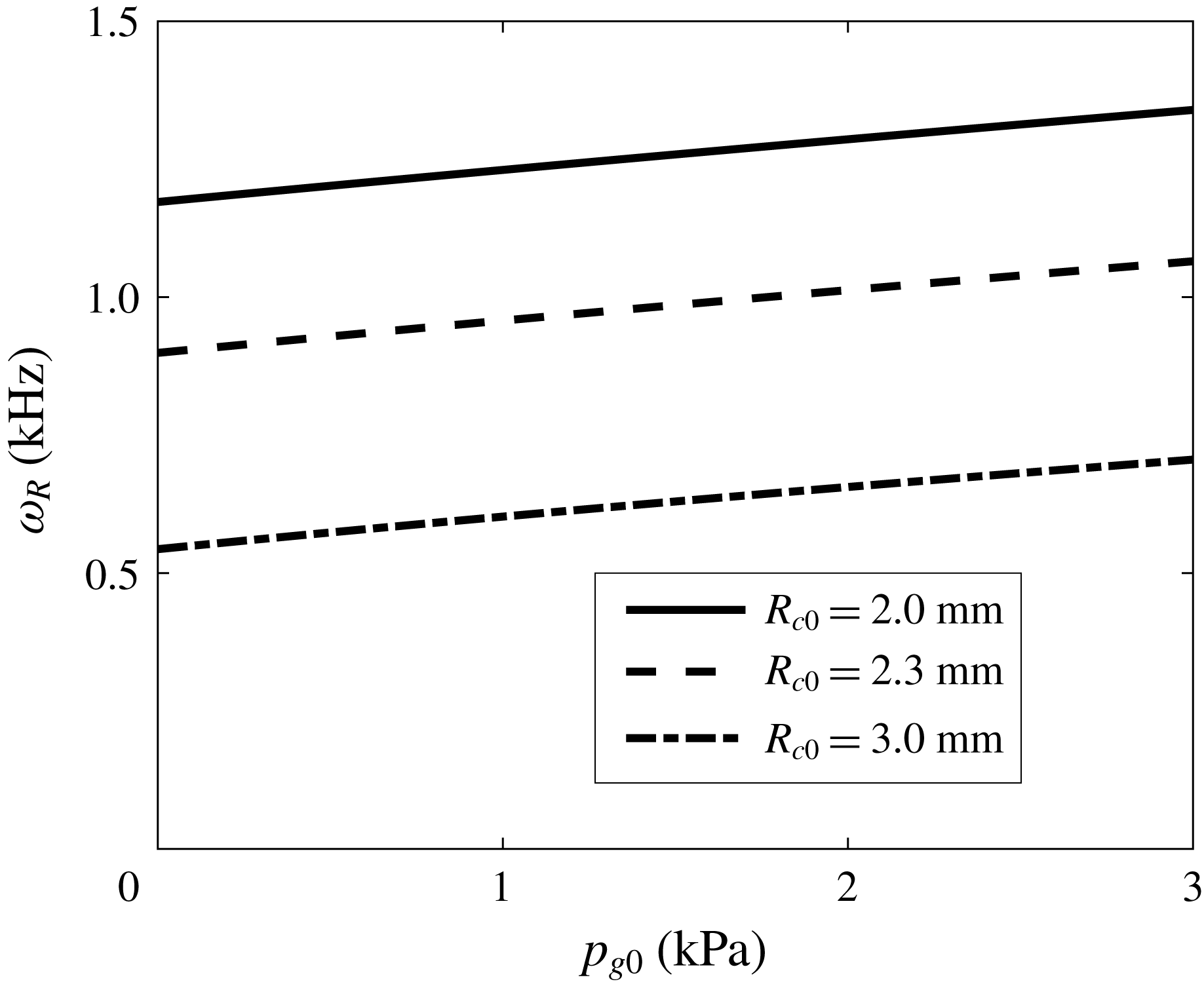
Firstly, we discuss the effects of the gas pressure. The initial partial pressure of gas is relevant to the dissolved gas in water, which is of significance in cavitation inception. For a developed cavitation bubble, on the other hand, the main contribution of gas pressure lies in changing the natural frequency. Figure 3 shows the variation of the natural frequency of the radial mode,
 $\unicode[STIX]{x1D714}_{R}$
, with respect to the initial gas pressure,
 $p_{g0}$
, according to (2.26). The cases for initial radius
 $R_{c0}=2.0$
, 2.3 and 3.0 mm are investigated. The gas pressure increases the natural frequency, while the effect is less important than that of the flow situation. These two effects could be compared by the ratio between the first and the third terms in (2.26), which is expressed as
 $(2\unicode[STIX]{x1D701}p_{g0})/(\unicode[STIX]{x1D70C}\unicode[STIX]{x1D70E}_{v}W^{2})$
by combining (3.1). The less important effect of gas pressure is also revealed by comparing the increased magnitude across the pressure range and the value at
 $p_{g0}=0$
. We can infer that it would not change the instability relation we will derive in § 3.5. To bypass the difficulty and uncertainty in determining the gas content, which is related to the practical water quality, and to refine the parameters that affect the stability condition, we will not discuss the effect of the partial pressure of gas in the following results and set the gas pressure to zero. The effect of this pressure can be easily included in our model if the incondensable air content is specified.
Natural frequency of radial mode
 $\unicode[STIX]{x1D714}_{R}$
versus the initial gas pressure
 $p_{g0}$
for the cylindrical cavitation bubble with initial radius
 $R_{c0}=2.0$
, 2.3 and 3.0 mm.

3.2 Effects of confinement
Next, we evaluate the effects of confinement by investigating the dependence of natural frequency or dispersion relation on the ratio between water tunnel radius,
 $R_{T}$
, and bubble radius,
 $R_{c0}$
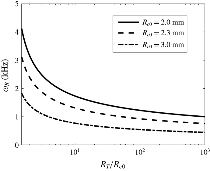
. We plot the variation of natural frequency of the radial mode versus different ratios
 $R_{T}/R_{c0}$
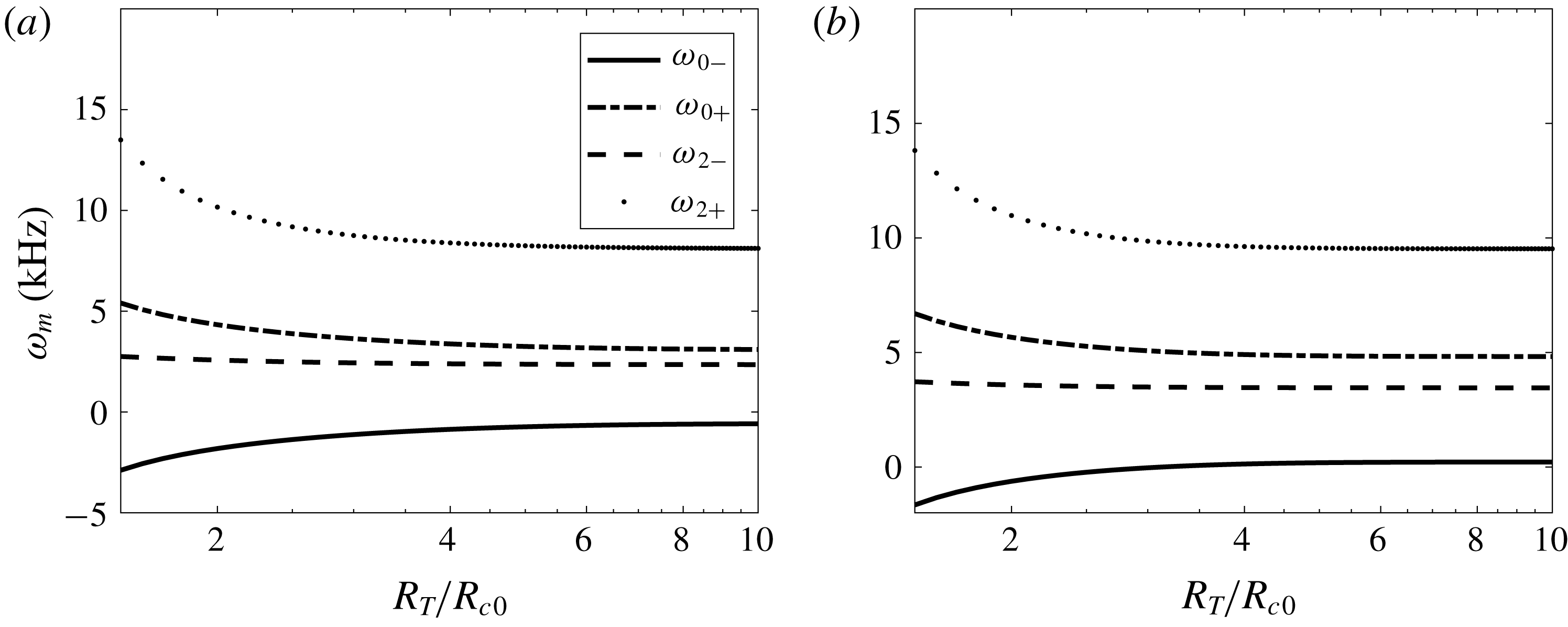
according to (2.26) in figure 4. For all the cases with different initial radii, the confinement increases the natural frequency appreciably when the tunnel size is smaller than 10 times the bubble size. The influence of confinement attenuates as the tunnel size increases. The curves exhibit little variation for
 $R_{T}/R_{c0}>100$
. The effect of confinement on the surface modes is restricted to a much smaller tunnel size, as indicated in figure 5. For the wavenumbers selected as examples,
 $k=200$
and
 $400~\text{m}^{-1}$
, the effect of confinement is obvious for
 $R_{T}/R_{c0}<4$
. Only the cases for surface modes
 $m=0^{\pm }$
and
 $2^{\pm }$
are displayed here, and other surface modes have similar characteristics.
Natural frequency of radial mode
 $\unicode[STIX]{x1D714}_{R}$
versus size ratio
 $R_{T}/R_{c0}$
for the cylindrical cavitation bubble with initial radius
 $R_{c0}=2.0$
, 2.3 and 3.0 mm.

Natural frequencies of surface modes
 $\unicode[STIX]{x1D714}_{m}$
(
 $m=0^{\pm }$
and
 $2^{\pm }$
) versus size ratio
 $R_{T}/R_{c0}$
for the cylindrical cavitation bubble with initial radius
 $R_{c0}=2.3$
mm under free-stream velocity
 $W=6.3~\text{m}~\text{s}^{-1}$
and wavenumber (a)
 $k=200~\text{m}^{-1}$
and (b)
 $k=400~\text{m}^{-1}$
.

In practice, most water tunnels have square cross-section with rounded corners to eliminate secondary flows. This shape can be approximately described as
 $r=R_{T}(1+\unicode[STIX]{x1D6FF}f)$
, in which
 $f$
could be a harmonic function. For example,
 $\unicode[STIX]{x1D6FF}=1/20$
and
 $f=\cos (4\unicode[STIX]{x1D703})$
with
 $0\leqslant \unicode[STIX]{x1D703}<2\unicode[STIX]{x03C0}$
is a proper choice for a square cross-section with rounded corners. Note that the effect of the non-circular shape is absent in the leading-order equation (2.24), which implies that the shape of the tunnel does not play any role in the radial model. Besides, it is easy to check that the fourth-order harmonic function is the lowest-order component to represent a square section. According to linear Fourier analysis, the perturbation of water tunnel shape only affects the corresponding harmonic component of the flow field due to the orthogonal properties of harmonic functions. Hence, the cross-section of a cavitation tunnel only affects the flow field relating to
 $\text{e}^{\text{i}m\unicode[STIX]{x1D703}}$
with
 $m\geqslant 4$
. Unless there is particular interest in high-order harmonics, we only consider a circular water tunnel of constant radius
 $R_{T}$
in this work.
In the experiment by Pennings et al. (Reference Pennings, Bosschers, Westerweel and van Terwisga2015), the cross-section of the water tunnel is
 $0.3~\text{m}\times 0.3~\text{m}$
. The distance to the nearest wall is approximately 100 times the bubble radius. Therefore, in the following analysis on surface stability, we neglect the effect of confinement on the surface mode and only solve the dynamic equations in § 2.3. Nevertheless, the dynamic model in § 2.4 is applicable for the cases with significant confinement effect, e.g. in microfluidics, which is not chosen as an example in the present paper. Note that the effect of confinement on the radial dynamics is always taken into account and is important in (2.24).
3.3 Effects of viscosity
In this section, the effects of viscosity are evaluated by investigating the eigenvalues (2.43) and (2.44) obtained from the dynamic equations with viscous stress in § 2.5. As mentioned, the imaginary parts of the eigenvalues are associated with the natural frequencies. On the other hand, the real parts are relevant to the decay or growth of the oscillatory amplitude, depending on whether values are positive or negative, respectively. If the viscosity is neglected (
 $\unicode[STIX]{x1D707}=0$
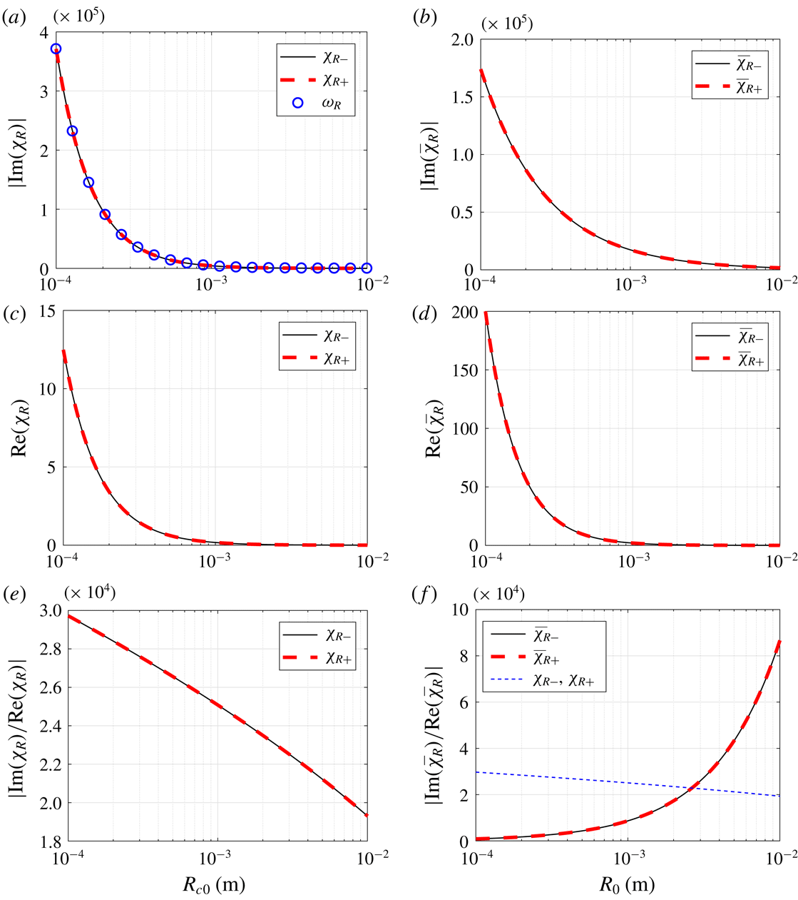
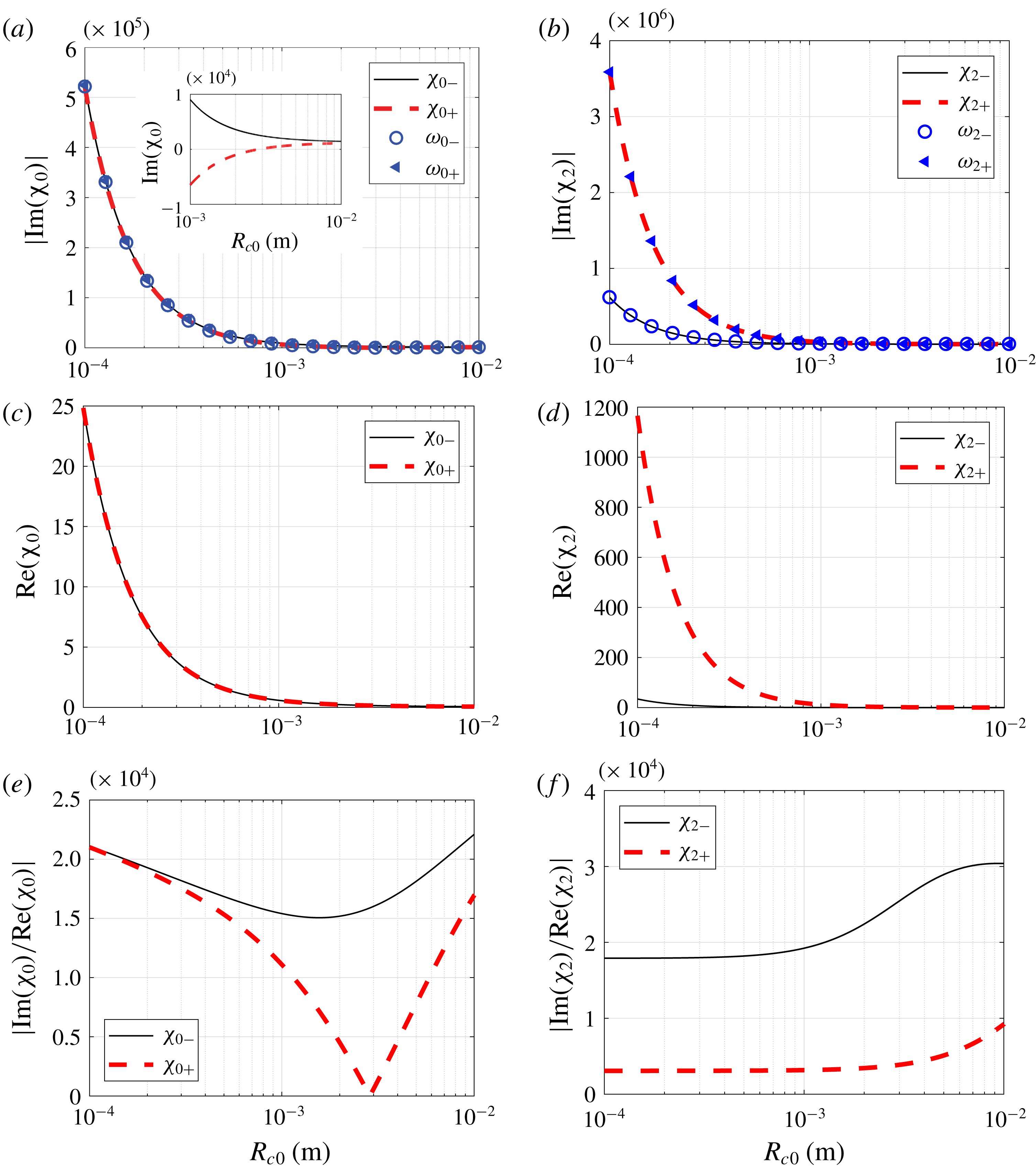
), the real parts of the eigenvalues are zero, implying an undamped oscillation. The imaginary parts, real parts and their ratios are plotted versus the bubble radius in figures 6 and 7 for the radial mode and surface modes, respectively.
For the radial mode, the positive and negative branches of the imaginary parts in (2.43) are exactly equal except for the sign. Hence, the two curves overlap as indicated in figure 6(a). The natural frequencies calculated by (2.26), which is without viscosity, are also denoted (blue circles) and present the same values as the eigenvalues which include the viscous effect, implying few effects of viscosity on the natural frequency. The real parts of the eigenvalues are always positive (figure 6
c), revealing the damping effect of viscosity. It is noted that this damping effect weakens with the bubble radius increasing. The ratio of the imaginary and real parts, shown in figure 6(e), is equivalent to the quality factor for an oscillator. This quantity represents the number of free oscillations before the amplitude decays to a negligible value (Fitzpatrick Reference Fitzpatrick2012). The quality factor for the vortex cavitation bubble decreases as the bubble radius increases. This phenomenon differs from a spherical bubble, for which the quality factor increases appreciably along with bubble size (Chapman & Plesset Reference Chapman and Plesset1971). For the sake of comparison, we plot the eigenvalues of a standard Rayleigh–Plesset equation for a spherical bubble within the same radius range in figure 6(b,d,f). The expressions of the characteristic equation and the eigenvalue are given in appendix D. For the spherical bubble, the natural frequency and damping effect are both smaller for larger bubbles, as shown in figure 6(b,d), which are similar to the cylindrical bubbles (figure 6
a,c). However, the variation of damping effect with respect to the spherical bubble radius is more apparent than that for cylindrical bubbles, referring to the coordinate value of figure 6(c,d). The damping effect overwhelms the oscillation when the spherical bubble becomes small. By comparison, the damping effect for the cylindrical bubble is one order smaller in magnitude. In other words, the viscous damping is less important for the cylindrical bubble than for the spherical bubble with comparable radii. In addition, the quality factor for the cylindrical bubble is around the order
 $O(10^{4})$
, a value much larger than 1. Although decreasing as the bubble size increases, it remains larger than that of a spherical bubble with radius smaller than 3 mm (cf. the dotted blue line in figure 6
f which is reproduced from figure 6
e). Therefore, the viscous effect on the radial oscillation for the cylindrical bubble investigated in the present work can be neglected.
The imaginary (a,b) and real (c,d) parts of the eigenvalue
 $\unicode[STIX]{x1D712}_{R}$
(2.43), and their ratio (e,f) versus radius for the vortex cavitation bubble (a,c,e) and the spherical bubble (b,d,f).

The imaginary (a,b) and real (c,d) parts of the eigenvalue
 $\unicode[STIX]{x1D712}_{m}$
(2.44), and their ratio (e,f) versus radius for
 $m=0$
(a,c,e) and
 $m=2$
(b,d,f).

For the surface modes, the natural frequencies, i.e. the imaginary parts of the eigenvalues (2.44), decrease with increasing bubble radius (figure 7
a,b). The curves are overlapped by the calculated natural frequencies without viscosity from (2.27), implying that the viscosity hardly affects the natural frequency of shape modes. Owing to the retrograde and co-grade branches of the dispersion relations, there are two separate curves for the two natural frequencies. This is not obvious for the mode
 $m=0$
but can be seen in the inset in figure 7(a) with local zoom. The inset shows that the absolute values of the retrograde and co-grade branches of the dispersion relation are different, and there is zero frequency for
 $m=0^{+}$
, which will be discussed below. The real parts of the eigenvalues are positive for both surface modes, representing the damping by viscosity. The damping effect attenuates for larger bubbles (figure 7
c,d). Note that the retrograde rotation of the angular velocity relative to the external flow has a less damping effect than the co-grade rotation for a non-axisymmetric mode,
 $m=2$
(figure 7
d). This is because the same direction of external flow relative to the angular velocity at the bubble interface tends to smooth the surface mode, and vice versa. In figure 7(e,f), we find that the quality factors for the surface modes do not vary monotonically. A zero quality factor appears in the mode
 $m=0^{+}$
. This point is related to the zero natural frequency, which can be seen from the inset in figure 7(a), implying the appearance of a stationary wave which was observed in Pennings et al. (Reference Pennings, Bosschers, Westerweel and van Terwisga2015). We should emphasize that the zero quality factor is yielded by zero natural frequency, but not by large damping. The associated damping effect is still small, referring to the associated value in figure 7(c).
Overall, the effect of viscosity is not important for the investigated cylindrical bubble in that: (i) the viscosity hardly changes the natural frequency; (ii) the damping effect, i.e. the real part of the eigenvalue, becomes small for the bubble with which we are concerned, with radius of the order of a millimetre; and (iii) the quality factor is mainly much larger than 1, while a value smaller than 1 is related to the zero natural frequency. Therefore, we neglect the effect of viscosity in the following discussion.
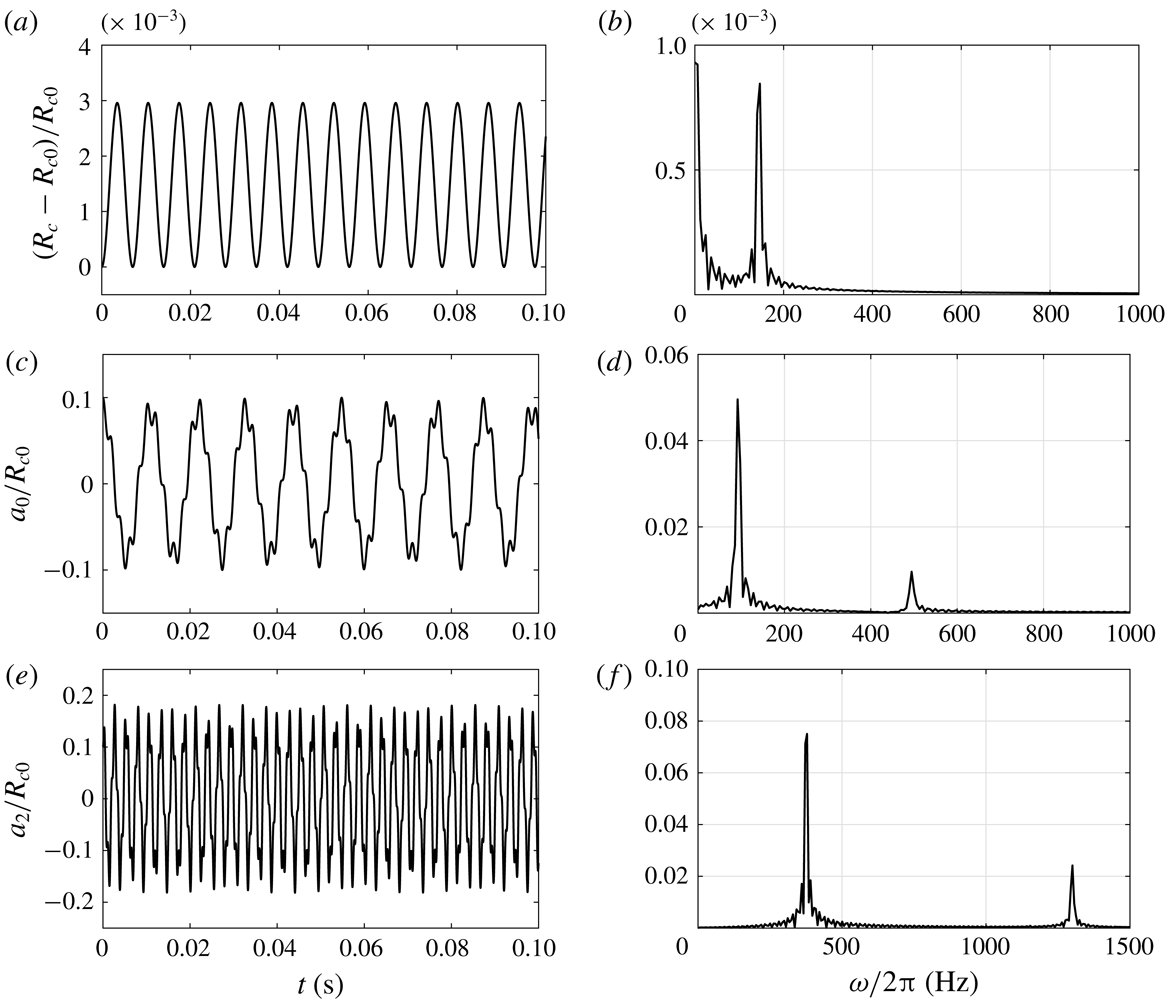
(a,c,e) Time evolutions of radial mode (a) and surface modes of
 $m=0$
(c) and
 $m=2$
(e) for a bubble with initial radius
 $R_{c0}=2.3$
mm under free-stream velocity
 $W=6.3~\text{m}~\text{s}^{-1}$
and wavenumber
 $k=200~\text{m}^{-1}$
. (b,d,f) The related FFT diagrams.

3.4 Validation of dynamics equations and dispersion relation
Through solving the dynamic equations (2.24) and (2.25), we can predict the evolutions of the radial and surface modes. Subject to the free-stream velocity
 $W=6.3~\text{m}~\text{s}^{-1}$
and wavenumber
 $k=200~\text{m}^{-1}$
, the time variations of the radius and surface modes of
 $m=0$
and 2 are displayed in figure 8(a,c,e). The related mode amplitudes in the frequency domain are obtained through fast Fourier transform (FFT) and shown in figure 8(b,d,f). The natural frequencies for the present bubble are calculated by (2.26) and (2.27) and listed in table 1. As shown in figure 8(a), the radius oscillates in harmonics under the present situation. Since the amplitude is small, of the order of
 $10^{-3}R_{c0}$
, its oscillatory frequency closely corresponds to the natural frequency by comparing the peak value in figure 8(b) and the calculated natural frequency in table 1. The oscillations of surface modes are not simply in harmonics, as shown in figure 8(c,d). From the FFT diagram, we find that two peaks are related to the retrograde and co-grade branches of the dispersion relations (2.25), respectively. The surface mode oscillates at the frequency combining these two natural frequencies. The FFT diagrams in figure 8(d,f) show that the amplitude related to the retrograde branch,
 $\unicode[STIX]{x1D714}_{m-}$
, of the natural frequency is larger than the co-grade branch,
 $\unicode[STIX]{x1D714}_{m+}$
. It is attributed to the concentrating or stretching of the surface modes when the phase velocity of the surface mode is opposing or following the background streamwise flows. This characteristic is also revealed in the damping effect we have discussed for figure 7(d).
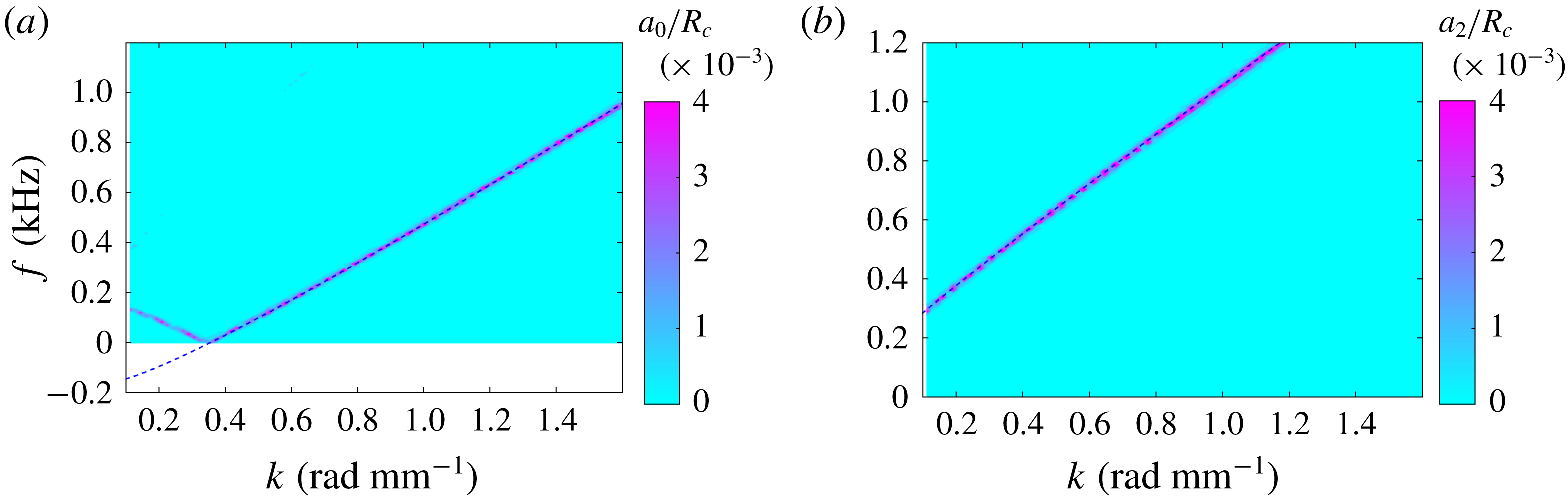
Pennings et al. (Reference Pennings, Bosschers, Westerweel and van Terwisga2015) obtained the relation between the wavenumber and the oscillatory frequency for surface modes by a two-dimensional FFT of high-speed video observations. Here we present the same diagram by solving our derived dynamic equations and carrying out the FFT analysis. Since the dynamic equations are decoupled for different surface modes, we plot the diagrams separately for
 $m=0$
in figure 9(a) and
 $m=2$
in figure 9(b). The colour denotes the amplitude of surface mode normalized by the mean radius
 $a_{m}/R_{c}$
(
 $m=0,2$
). The dashed lines are obtained according to the dispersion relation (2.27). We find that the frequencies at different wavenumbers overlap the peaks of the FFT results of the surface mode amplitudes. It is noted that only the retrograde branch of the dispersion relation is presented since the amplitude for the co-grade branch is much smaller. These characteristics agree well with the observation by Pennings et al. (Reference Pennings, Bosschers, Westerweel and van Terwisga2015, figure 10 therein), implying that our derived equations can predict the dynamics of surface modes.
Natural frequencies for the bubble with the parameters given in figure 8.


3.5 Stability of surface modes
To analyse the stability of the surface mode, we revisit the dynamic equation (2.25). The coefficients in this linear oscillatory equation include the variation of the mean radius
 $R_{c}$
and its time derivative. We assume the radius oscillates at an infinitesimal amplitude
 $\unicode[STIX]{x1D716}$
,
 $$\begin{eqnarray}R_{c}(t)=R_{c0}(1+\unicode[STIX]{x1D716}\text{e}^{\text{i}\unicode[STIX]{x1D714}_{d}t}),\end{eqnarray}$$
where
 $\unicode[STIX]{x1D714}_{d}$
is the angular frequency of oscillation, which is determined by external flow. Note that
 $\unicode[STIX]{x1D714}_{d}$
is not necessarily equal to the natural frequency of the radial mode,
 $\unicode[STIX]{x1D714}_{R}$
. The term with time derivative of the radius,
 ${\dot{R}}_{c}$
, in the coefficient before
 ${\dot{a}}_{m}$
in (2.25) is strictly kinematic in origin (Leal Reference Leal2007). Its destabilizing (stabilizing) effect is clearly related to the converging (diverging) nature of the streamlines for the radial motion. Therefore, we do not discuss the terms with
 ${\dot{R}}_{c}$
in the coefficient before
 ${\dot{a}}_{m}$
and eliminate them temporarily. Let
 $a_{m}=\text{e}^{-\unicode[STIX]{x1D705}t}\unicode[STIX]{x1D709}_{m}$
, where
 $\unicode[STIX]{x1D705}=\text{i}(kW+(m\unicode[STIX]{x1D6E4}/2\unicode[STIX]{x03C0}R_{c}^{2}))$
. Accordingly, equation (2.25) becomes
 $$\begin{eqnarray}\displaystyle \ddot{\unicode[STIX]{x1D709}}_{m}+\left[\frac{\left(\unicode[STIX]{x1D714}_{m}-kW-{\displaystyle \frac{m\unicode[STIX]{x1D6E4}}{2\unicode[STIX]{x03C0}R_{c}^{2}}}\right)^{2}}{\unicode[STIX]{x1D714}_{d}^{2}}+\frac{F(R_{c})}{\unicode[STIX]{x1D714}_{d}^{2}}\right]\unicode[STIX]{x1D709}_{m}=0, & & \displaystyle\end{eqnarray}$$
where
 $F(R_{c})$
is a function related to
 $R_{c}$
, whose expression can be easily obtained from (2.25) as
 $$\begin{eqnarray}F(R_{c})=\frac{\ddot{R}_{c}}{R_{c}}-\frac{{\dot{R}}_{c}^{2}}{R_{c}^{2}}+\text{i}kW\frac{{\dot{R}}_{c}}{R_{c}}-\text{i}\frac{m\unicode[STIX]{x1D6E4}{\dot{R}}_{c}}{2\unicode[STIX]{x03C0}R_{c}^{3}}-\frac{\text{H}_{m}^{1\prime }(\text{i}kR_{c})}{\text{H}_{m}^{1}(\text{i}kR_{c})}\left(-\frac{{\dot{R}}_{c}^{2}}{R_{c}}-\ddot{R}_{c}-\text{i}\frac{m\unicode[STIX]{x1D6E4}}{2\unicode[STIX]{x03C0}R_{c}^{2}}{\dot{R}}_{c}-\text{i}kW{\dot{R}}_{c}\right).\end{eqnarray}$$
The overdot in (3.3) denotes differentiation with respect to time scale
 $\unicode[STIX]{x1D70F}$
, where
 $\unicode[STIX]{x1D70F}=\unicode[STIX]{x1D714}_{d}t$
. Substituting (3.2), the real part of (3.3) is written as
 $$\begin{eqnarray}\displaystyle \ddot{\unicode[STIX]{x1D709}}_{m}+\left[\frac{\left(\unicode[STIX]{x1D714}_{m}-kW-{\displaystyle \frac{m\unicode[STIX]{x1D6E4}}{2\unicode[STIX]{x03C0}R_{c}^{2}}}\right)^{2}}{\unicode[STIX]{x1D714}_{d}^{2}}+\unicode[STIX]{x1D716}M\cos \unicode[STIX]{x1D70F}\right]\unicode[STIX]{x1D709}_{m}=0, & & \displaystyle\end{eqnarray}$$
where
 $$\begin{eqnarray}M=-1-\frac{kW}{\unicode[STIX]{x1D714}_{d}}+\frac{m\unicode[STIX]{x1D6E4}}{2\unicode[STIX]{x03C0}\unicode[STIX]{x1D714}_{c}R_{c0}^{2}}-\frac{\text{H}_{m}^{1\prime }(\text{i}kR_{c})}{\text{H}_{m}^{1}(\text{i}kR_{c})}\left(R_{c0}+\frac{m\unicode[STIX]{x1D6E4}}{2\unicode[STIX]{x03C0}R_{c0}\unicode[STIX]{x1D714}_{d}}+\frac{kWR_{c0}}{\unicode[STIX]{x1D714}_{d}}\right).\end{eqnarray}$$
Equation (3.5) has the standard form of Mathieu’s equation. Therefore, the condition for the parametric instability is (Bender & Orszag Reference Bender and Orszag1999)
 $$\begin{eqnarray}\frac{\left(\unicode[STIX]{x1D714}_{m}-kW-{\displaystyle \frac{m\unicode[STIX]{x1D6E4}}{2\unicode[STIX]{x03C0}R_{c}^{2}}}\right)^{2}}{\unicode[STIX]{x1D714}_{d}^{2}}=\frac{n^{2}}{4},\end{eqnarray}$$
when
 $n$
is a natural number. It is noted that the numerator is not the natural frequency of surface modes (2.27), but its value subtracted by
 $kW+(m\unicode[STIX]{x1D6E4}/2\unicode[STIX]{x03C0}R_{c}^{2})$
, which is related to the basic vortical flow. The Mathieu structure in the dynamic equation implies that the surface mode may be triggered by the oscillation of the radial mode when its oscillatory frequency
 $\unicode[STIX]{x1D714}_{d}$
and the natural frequency of the surface mode
 $\unicode[STIX]{x1D714}_{m}$
satisfy the relation (3.7) when
 $n$
is a natural number, especially for
 $n=1$
.
Time evolutions of surface mode
 $m=0$
under the radial oscillation prescribed as
 $R_{c}(t)=R_{c0}[1+\unicode[STIX]{x1D716}\cos (\unicode[STIX]{x1D714}_{d}t)]$
with
 $\unicode[STIX]{x1D714}_{d}/2\unicode[STIX]{x03C0}=300$
Hz and (a)
 $\unicode[STIX]{x1D716}=0.57$
and (b)
 $\unicode[STIX]{x1D716}=0.58$
. The remaining parameters are the same as in figure 8.

The stability of the surface mode can be evaluated by sweeping the oscillatory frequency of radial mode,
 $\unicode[STIX]{x1D714}_{d}$
, and recording its threshold amplitude, denoted as
 $\unicode[STIX]{x1D716}_{thr}$
, beyond which an unstable surface oscillation occurs. Take an example of a bubble with initial radius
 $R_{c0}=2.3$
mm and wavenumber
 $k=200~\text{m}^{-1}$
. We impose a radial oscillation (3.2) and apply a frequency of
 $\unicode[STIX]{x1D714}_{d}/2\unicode[STIX]{x03C0}=300$
Hz. When the oscillatory amplitude
 $\unicode[STIX]{x1D716}=0.57$
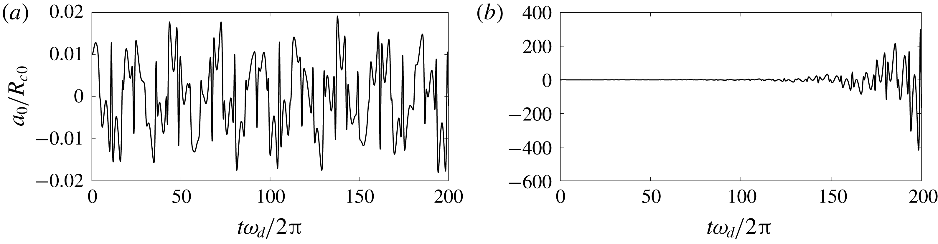
, the surface mode
 $m=0$
oscillates in a stable manner. As shown in figure 10(a), the oscillation keeps a finite amplitude as time progresses. When the amplitude increases slightly, e.g.
 $\unicode[STIX]{x1D716}=0.58$
, the initial disturbance to the surface mode increases explosively and the surface mode becomes unstable, as shown in figure 10(b). For this case, we denote the amplitude threshold that induces surface instability as
 $\unicode[STIX]{x1D716}_{thr}=0.58$
.
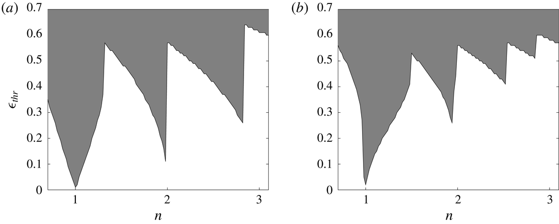
Next we plot the stability diagram in figure 11 for the bubble whose parameters are the same as in figure 8 for the case of the surface modes
 $m=0$
and 2. For this bubble,
 $(\unicode[STIX]{x1D714}_{m}-kW-(m\unicode[STIX]{x1D6E4}/2\unicode[STIX]{x03C0}R_{c}^{2}))/2\unicode[STIX]{x03C0}$
is calculated to be 293 Hz and 458 Hz for
 $m=0$
and 2, respectively. Sweeping the radial frequency
 $\unicode[STIX]{x1D714}_{d}$
, we obtain various
 $n$
(not necessarily a natural number). Recording the related amplitude threshold with respect to
 $n$
illustrates the stability diagram. We find that a global minimum appears at
 $n=1$
and a secondary minimum at
 $n=2$
. This is analogous to the one–two and one–one resonances for the shape modes of a spherical bubble, which were discussed by Feng & Leal (Reference Feng and Leal1993) and Yang et al. (Reference Yang, Feng and Leal1993). It is essentially the energy transfer between the radial mode and surface mode when the resonant relation is satisfied. They are regarded as the most unstable situations for the Mathieu-type instability. The amplitude threshold
 $\unicode[STIX]{x1D716}_{thr}$
is smaller for
 $m=0$
than that for
 $m=2$
at the resonance when
 $n=1$
and 2. This implies that the energy transfer due to resonance is likely to occur for lower-order surface mode, which is reasonable for the Mathieu-type instability. The local minimum for
 $n>2$
is not exactly at the natural number points. The reason is that the Mathieu-type instability is substantially valid when
 $\unicode[STIX]{x1D716}$
in (3.5) is infinitesimal. With the oscillatory frequency increasing, the surface mode tends to become stable due to there being insufficient time for the development of the surface instability under quick oscillation. Hence the instability threshold increases generally for higher oscillatory frequencies. Nevertheless, the stability diagram figure 11 confirms our derivation that the dynamic equation of the surface mode bears the structure of Mathieu’s equation.
Stability diagram of the bubble for the surface modes (a)
 $m=0$
and (b)
 $m=2$
. The remaining parameters are the same as in figure 8.

3.6 Developments of surface modes
From the stability diagram in figure 11, we know that instability of surface modes may occur at resonance or when the oscillatory amplitude of the radial mode is large enough. If the bubble is stationary initially, i.e.
 ${\dot{R}}_{c}(t=0)=0$
and
 $\ddot{R}_{c}(t=0)=0$
, which is the initial condition we assigned in the previous sections, the bubble is always at a nearly equilibrium state. This can be revealed by recalling (2.24) and setting
 ${\dot{R}}_{c}$
and
 $\ddot{R}_{c}$
zero, which yields
 $$\begin{eqnarray}\frac{1}{\unicode[STIX]{x1D70C}}\left[p_{v}+p_{g0}\left(\frac{R_{c0}}{R_{c}}\right)^{2\unicode[STIX]{x1D701}}+\frac{\unicode[STIX]{x1D70E}}{R_{c}}-p_{T}\right]=\frac{1}{\unicode[STIX]{x1D70C}}(p_{v}-p_{T})\left(1-\frac{R_{c}^{2}}{R_{T}^{2}}\right).\end{eqnarray}$$
If the size of the water tunnel is much larger than the bubble radius, the partial pressure of gas is neglected and the surface tension is not significant, which are true in the present cases, the bubble radius
 $R_{c}$
always approximates to its initial size
 $R_{c0}$
. The above results, e.g. figure 8(a), show the small amplitude of radial oscillation under the present situation. This small radial amplitude is usually insufficient to trigger surface modes according to the above stability analysis.
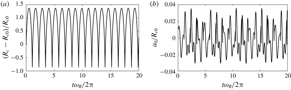
Time evolutions of (a) radial mode and (b) surface modes of
 $m=0$
for
 ${\dot{R}}_{c0}=2.55~\text{m}~\text{s}^{-1}$
(case
 ${\mathcal{A}}$
). The remaining parameters are the same as in figure 8.


In fact, the formation of vortex cavitation involves a dramatic phase transition. Although phase change is not included in our model, it causes the radial velocity due to cavitation inception at the order of
 $5~\text{m}~\text{s}^{-1}$
for a vapour core of 1 mm diameter (Franc & Michel Reference Franc and Michel2010). This kind of disturbance makes the bubble oscillate appreciably in radius, which has the potential for inducing surface instability.
Hereafter, we prescribe an initial radial velocity and increase it from zero in steps of
 $0.5~\text{m}~\text{s}^{-1}$
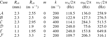
to find the threshold of initial radial velocity that induces the instability of surface modes. The parameters for the cases we will investigate are listed in table 2. Firstly, we investigate the bubble with the same flow parameters as in figure 8. When the initial radial velocity increases up to
 $2.55~\text{m}~\text{s}^{-1}$
(case
 ${\mathcal{A}}$
), the surface mode of
 $m=0$
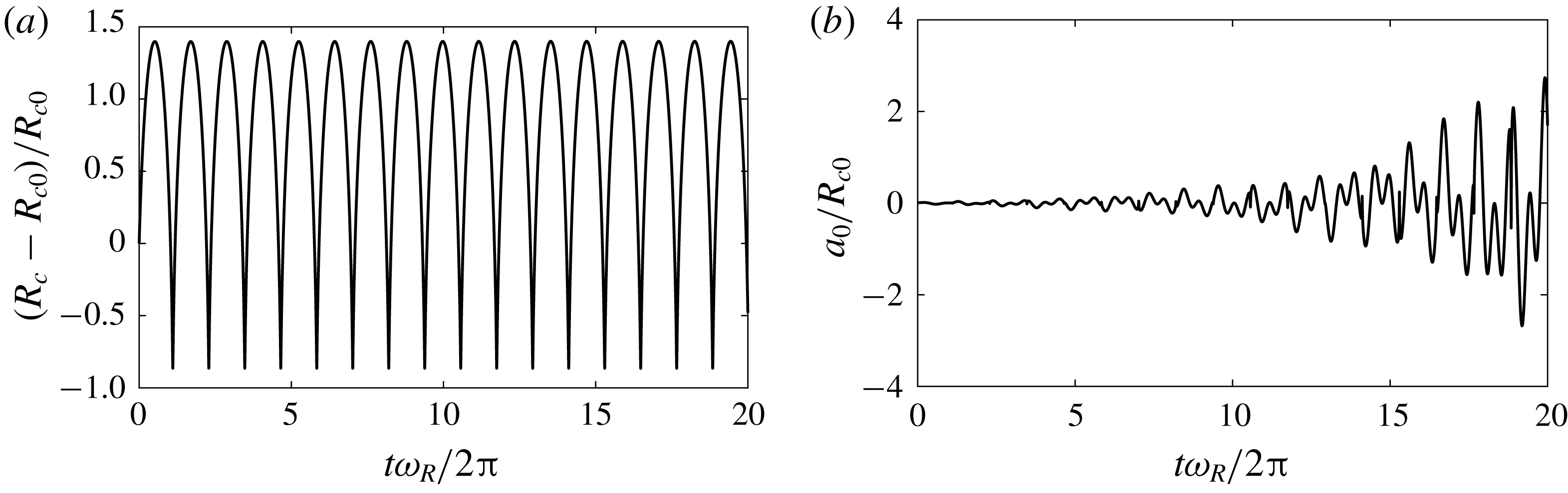
becomes unstable, as shown in figure 12(b). The associated radial oscillation is presented in figure 12(a), which is nonlinear with a slow growth followed by a sharp collapse. If the initial radial velocity is a little smaller, e.g.
 ${\dot{R}}_{c0}=2.5~\text{m}~\text{s}^{-1}$
(case
 ${\mathcal{B}}$
), the zeroth-order surface mode is stable (figure 13
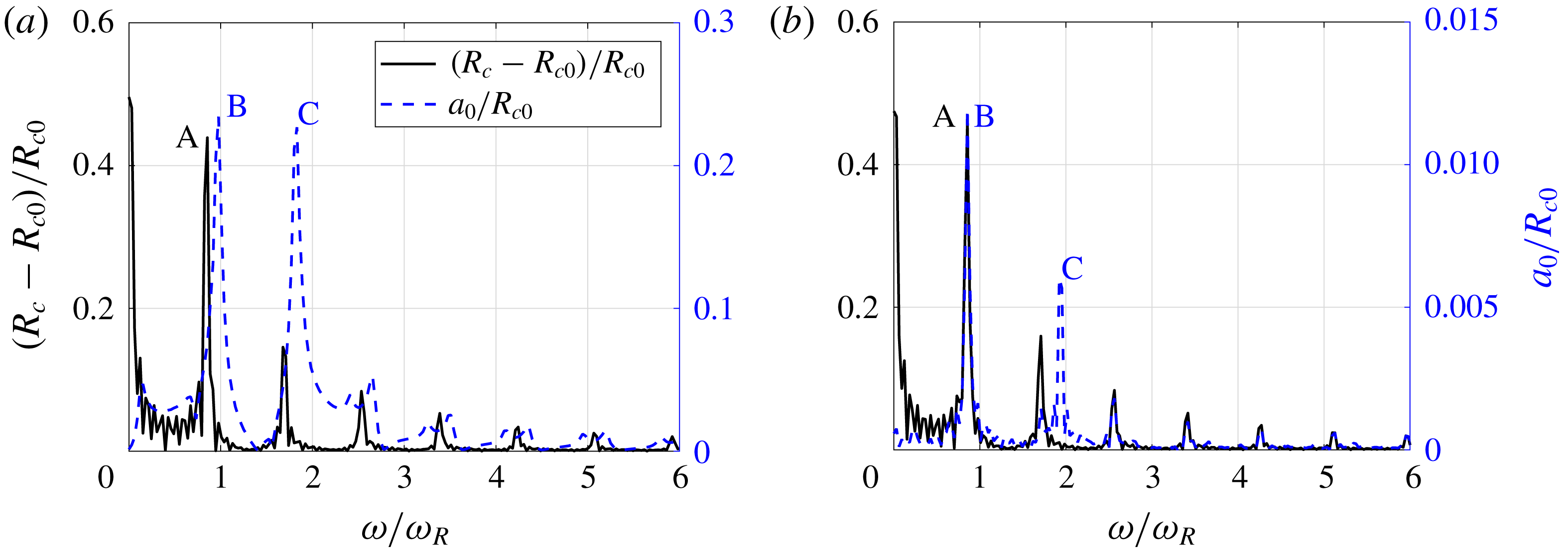
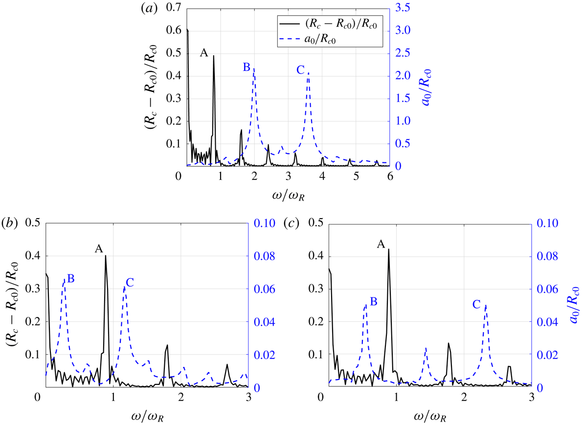
b), i.e. the initial disturbance to the surface mode is not amplified continuously like the case in figure 12(b). The FFTs of the radial and surface oscillations are presented in figure 14 for the above unstable and stable cases. Owing to the linear analysis of the surface oscillation in the present work, the absolute magnitude of the amplitude of the surface mode
 $a_{0}$
lacks physical meaning. Nevertheless, the peak in the FFT diagram reveals the dominant frequency when the surface mode develops. In figure 14(b), the first peak of the surface mode, denoted as B in the figure, overlaps the peak of the radial mode, denoted as A. However, for this case, the instability of the relevant surface mode does not emerge (figure 13
b). The frequencies of the peak for the radial mode (point A) and the two peaks for the surface mode (points B and C) are recorded in table 2 as well. This demonstrates that the surface instability is not triggered by the direct resonance between radial mode and surface mode at the natural frequencies. Turning to the unstable case, case
 ${\mathcal{A}}$
and figure 14(a), the peak of the radial mode (A) does not overlap with any peak of the surface mode (B or C). But if we subtract
 $(1/2\unicode[STIX]{x03C0})(kW+(m\unicode[STIX]{x1D6E4}/2\unicode[STIX]{x03C0}R_{c}^{2}))$
, which is calculated to be 200.5 Hz for case
 ${\mathcal{A}}$
, from the frequencies at points B and C, we obtain
 $-64.5$
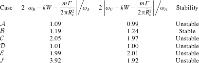
Hz and 58.4 Hz, respectively. By referring to the value at point A, 118.5 Hz, the calculated values satisfy the instability condition (3.7) with
 $n\,\approx \,1$
(see table 3). It should be mentioned that the frequency values at point A for cases
 ${\mathcal{A}}$
,
 ${\mathcal{B}}$
and
 ${\mathcal{C}}$
are different, although for the same bubble, and also deviate from the calculated frequency 143.9 Hz by (2.26). The reason is that the radial oscillation is nonlinear under given initial velocities, such as figures 12(a) and 13(a), making the averaged radius differ among them, and distinguish from the one obtained by (2.26) using initial radius.
Furthermore, we investigate more cases with wavenumber
 $k=400~\text{m}^{-1}$
and/or for initial radius
 $R_{c0}=1.1$
mm, cases
 ${\mathcal{C}}$
,
 ${\mathcal{D}}$
and
 ${\mathcal{E}}$
. The parameters are selected by referring to Pennings et al. (Reference Pennings, Bosschers, Westerweel and van Terwisga2015). For these three cases, the surface mode
 $m=0$
is unstable, which is induced by the radial velocity list in table 2. Similar phenomena are found from the FFT diagrams of radial mode and unstable surface mode as shown in figure 15. For these cases, the peak frequencies at points B and C minus
 $(1/2\unicode[STIX]{x03C0})(kW+(m\unicode[STIX]{x1D6E4}/2\unicode[STIX]{x03C0}R_{c}^{2}))$
and divided by the peak frequency at point A satisfy (3.7) for
 $n\approx 1$
or 2 (see table 3), which are the two most unstable conditions according to the stability diagram as shown in figure 11.
Time evolutions of (a) radial mode and (b) surface modes of
 $m=0$
for
 ${\dot{R}}_{c0}=2.5~\text{m}~\text{s}^{-1}$
(case
 ${\mathcal{B}}$
). The remaining parameters are the same as in figure 8.

The stabilities for the cases in table 2.


The FFT diagram of radial mode (black solid line) and surface mode (blue dashed line) related to (a) case
 ${\mathcal{C}}$
, (b) case
 ${\mathcal{D}}$
and (c) case
 ${\mathcal{E}}$
.

Time evolutions of radial mode (a) and surface mode (b) for case
 ${\mathcal{F}}$
and the related FFT diagram (c).

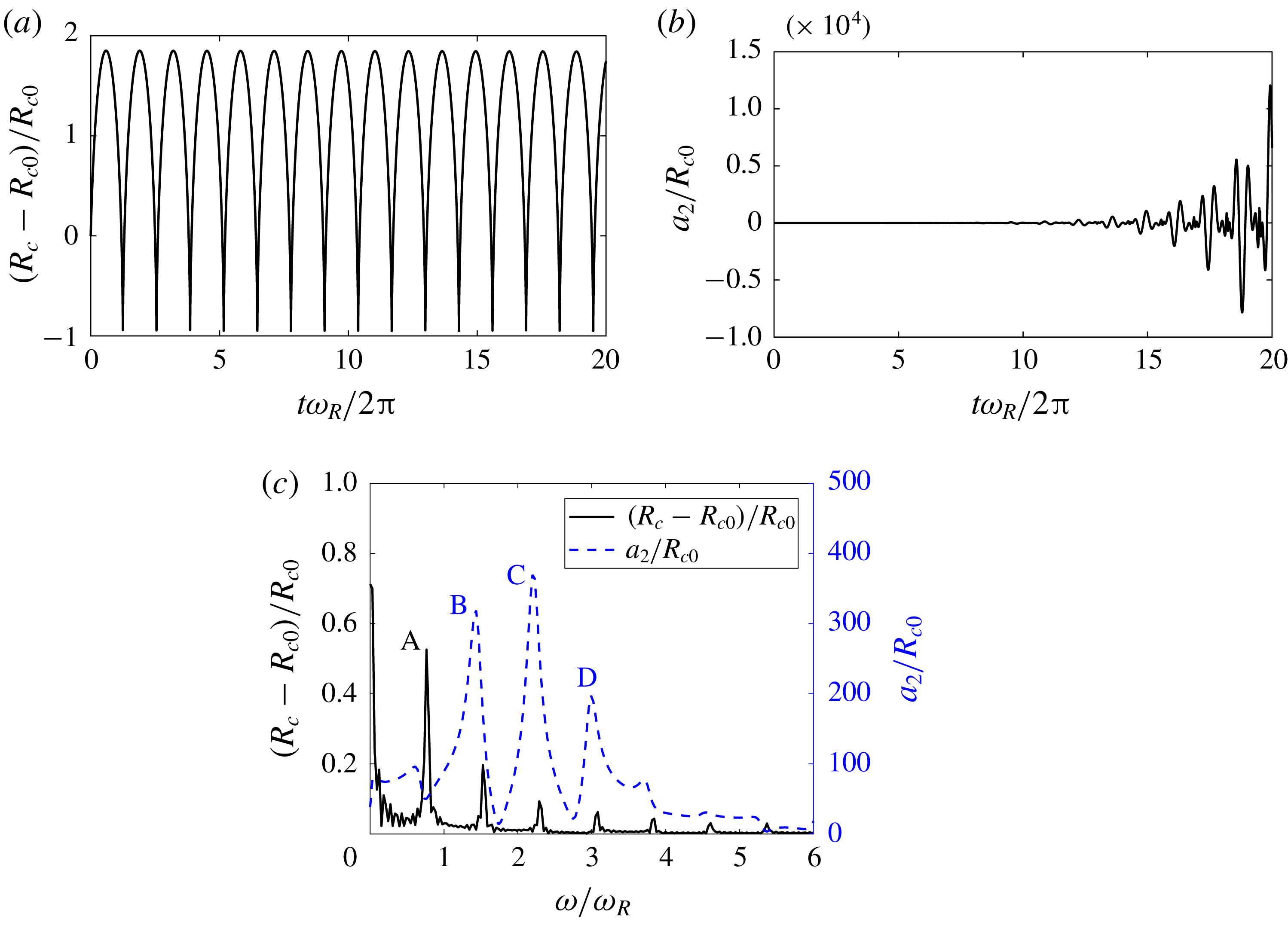
Concerning the surface mode of
 $m=2$
, the minimal radial velocity that induces the surface instability for the bubble increases to
 $3.3~\text{m}~\text{s}^{-1}$
, denoted as case
 ${\mathcal{F}}$
. With this radial velocity, the radial oscillation exhibits nonlinear characteristics (figure 16
a), and the second-order surface mode becomes unstable (figure 16
b). The relevant FFT diagram is shown in figure 16(c). At first, we substitute the frequencies at points A, B and C, along with the initial radius
 $R_{c0}=2.3$
mm, axial velocity
 $W=6.3~\text{m}~\text{s}^{-1}$
, wavenumber
 $k=200~\text{m}^{-1}$
and circulation
 $\unicode[STIX]{x1D6E4}=0.066~\text{m}^{2}~\text{s}^{-1}$
, into (3.7), and obtain
 $n=11.4$
and 9.3 for
 $f_{B}$
and
 $f_{C}$
, respectively, which seems that the instability condition (3.7) is not satisfied for this case since
 $n$
is not a natural number. The reason is probably that the radial oscillation is nonlinear, which makes the averaged radius deviate from the initial one, so that the error yields when calculating
 $kW+(m\unicode[STIX]{x1D6E4}/2\unicode[STIX]{x03C0}R_{c}^{2})$
(note that the second term is zero for the mode
 $m=0$
). The value at
 $\unicode[STIX]{x1D714}=0$
in FFT diagram figure 16(c) denotes the averaged radius, calculated to be 3.9 mm accordingly. We use this averaged radius to re-evaluate the instability condition (3.7) and obtain that
 $n=3.92$
and 1.92 with respect to
 $f_{B}$
and
 $f_{C}$
, respectively. The instability condition (3.7) is acceptably satisfied based on the averaged radius. In addition, the time scale of surface oscillation is comparable with that of radial oscillation. Accordingly, we regard the stability as the Mathieu type. The instability can be induced when the oscillations of the radial and surface modes are modulated to meet a resonance condition.
We summarize the above-mentioned relations between the peak frequencies of the surface mode and radial mode, and the relevant stability in table 3. The second and third columns are actually
 $n$
in (3.7), the value of which is close to a natural number for the unstable cases. Therefore, we conclude that the surface instability of a cylindrical cavitation bubble has the characteristics of the Mathieu-type instability. First, the unstable condition (3.7) is perfectly satisfied when the averaged radius of the cylindrical bubble is considered. Second, the time scales of radial oscillation and surface oscillation are comparable when the surface instability is developing, which implies the possibility of resonance between radial and surface modes. This is the nature of Mathieu-type instability. Third, the lower surface mode is easier to be induced, which is revealed by the larger initial radial velocity to trigger the
 $m=2$
mode than the
 $m=0$
mode, agreeing with the characteristics of the Mathieu-type instability.
As mentioned in § 2, gravity is neglected in the momentum equation (2.11). Herein we compare gravity with the inertial force and transient effect. In principle, the Froude number, measuring the ratio of inertial force and gravity, is defined as
 $Fr^{2}=u_{\unicode[STIX]{x1D703}}^{2}/gR_{c0}$
. According to (3.1), the leading order of azimuthal velocity
 $u_{\unicode[STIX]{x1D703}}\sim \sqrt{\unicode[STIX]{x1D70E}_{v}}W$
. The magnitude of
 $Fr^{2}=\unicode[STIX]{x1D70E}_{v}W^{2}/gR_{c0}$
is of the order of
 $10^{3}$
, suggesting that gravity will not affect the pressure distribution and vortex structure. On the other hand, the transient effect is justified by
 $u_{r}\,f/g={\dot{R}}_{c0}\unicode[STIX]{x1D714}_{A}/2\unicode[STIX]{x03C0}g\sim O(30{-}50)$
according to the numerical results as shown in table 2. Therefore, for the cylindrical bubble oscillating at the present frequency range, gravity can be reasonably neglected.
4 Conclusions
In this paper, we have formulated the dynamic equations of the surface modes, in addition to the radial mode described by the well-known Rayleigh–Plesset equation, for a cylindrical cavitation bubble with and without the confinement of a water tunnel. The bubble is subject to a vortical flow with a constant axial velocity.
We derive an explicit expression for the dispersion relation of the surface mode. The effect of confinement on the surface mode is included in our model, whereas it is proved to be negligible unless the radius of the water tunnel,
 $R_{T}$
, is not large compared to the bubble radius,
 $R_{c}$
, e.g.
 $R_{T}/R_{c}<4$
. The viscous effect is investigated and judged to be unimportant for the present vortex cavitation bubble concerning the small damping coefficient and large quality factor. Our model is validated by comparison with the experiments by Pennings et al. (Reference Pennings, Bosschers, Westerweel and van Terwisga2015) and shows a good agreement, implying that our model can predict the dynamics of surface modes.
Furthermore, it is found that the dynamic equation of the surface mode has the structure of Mathieu’s equation and the instability condition for the surface mode is
 $(\unicode[STIX]{x1D714}_{m}-kW-(m\unicode[STIX]{x1D6E4}/2\unicode[STIX]{x03C0}R_{c}^{2}))^{2}/\unicode[STIX]{x1D714}_{d}^{2}=n^{2}/4$
, where
 $n$
is a natural number. The most unstable situation happens when
 $n=1$
, which is shown by a stability diagram. An initial radial velocity, which induces appreciable radial oscillation, is one of the mechanisms to trigger the surface modes. Justified by a few numerical examples, we prove that the condition (3.7) holds when the surface mode oscillation emerges, further demonstrating that the Mathieu-type instability contributes to the appearances of surface modes.
In the life of a bubble, the rebound phases of the radial and surface oscillations produce the most significant acoustic pressure. Meanwhile, the instability of surface modes lead to the breakup of a cylindrical bubble, resulting in rapid changes of the volume acceleration and radial velocity. The Mathieu-type formulation helps to identify the instability regime, which will guide the optimal design of various hydrofoils and propellers.
Acknowledgement
This research has been partially funded by National Natural Science Foundation of China (grant nos. 11772196, 11772195 and 91852204).
Appendix A. Derivation of the kinematic boundary condition at bubble interface
Let
 $C=kz+m\unicode[STIX]{x1D703}$
; the surface function (2.2) is written as
 $S=r-R_{c}(t)-\unicode[STIX]{x1D700}a_{m}(t)\text{e}^{\text{i}C}$
. The terms in the kinematic boundary condition (2.16) are written out separately as
 $$\begin{eqnarray}\displaystyle & \displaystyle \frac{\unicode[STIX]{x2202}S}{\unicode[STIX]{x2202}t}=-{\dot{R}}_{c}-\unicode[STIX]{x1D700}{\dot{a}}_{m}\text{e}^{\text{i}C}, & \displaystyle\end{eqnarray}$$
 $$\begin{eqnarray}\displaystyle & \displaystyle \unicode[STIX]{x1D735}S=\boldsymbol{e}_{r}-\text{i}\unicode[STIX]{x1D700}m\frac{a_{m}}{r}\text{e}^{\text{i}C}\boldsymbol{e}_{\unicode[STIX]{x1D703}}-\text{i}\unicode[STIX]{x1D700}ka_{m}\text{e}^{\text{i}C}\boldsymbol{e}_{z}, & \displaystyle\end{eqnarray}$$
 $$\begin{eqnarray}\displaystyle & \displaystyle \boldsymbol{u}=\left(\frac{R_{c}{\dot{R}}_{c}}{r}+\unicode[STIX]{x1D700}\frac{\unicode[STIX]{x2202}\unicode[STIX]{x1D719}}{\unicode[STIX]{x2202}r}\text{e}^{\text{i}C}\right)\boldsymbol{e}_{r}+\left(V_{\unicode[STIX]{x1D703}}+\text{i}\unicode[STIX]{x1D700}\frac{m}{r}\unicode[STIX]{x1D719}\text{e}^{\text{i}C}\right)\boldsymbol{e}_{\unicode[STIX]{x1D703}}+(W+\text{i}\unicode[STIX]{x1D700}k\unicode[STIX]{x1D719}\text{e}^{\text{i}C})\boldsymbol{e}_{z}, & \displaystyle\end{eqnarray}$$
 $$\begin{eqnarray}\displaystyle \boldsymbol{u}\boldsymbol{\cdot }\unicode[STIX]{x1D735}S & = & \displaystyle \frac{R_{c}{\dot{R}}_{c}}{r}+\unicode[STIX]{x1D700}\text{e}^{\text{i}C}\left[\frac{\unicode[STIX]{x2202}\unicode[STIX]{x1D719}}{\unicode[STIX]{x2202}r}-\text{i}mV_{\unicode[STIX]{x1D703}}\frac{a_{m}}{r}-\text{i}ka_{m}W\right]\nonumber\\ \displaystyle & = & \displaystyle {\dot{R}}_{c}+\unicode[STIX]{x1D700}\text{e}^{\text{i}C}\left[-\frac{{\dot{R}}_{c}}{R_{c}}a_{m}+\frac{\unicode[STIX]{x2202}\unicode[STIX]{x1D719}}{\unicode[STIX]{x2202}r}-\text{i}mV_{\unicode[STIX]{x1D703}c}\frac{a_{m}}{R_{c}}-\text{i}ka_{m}W\right].\end{eqnarray}$$
Substituted into (2.16), the kinematic boundary condition at the bubble interface is written as
 $$\begin{eqnarray}-{\dot{a}}_{m}-\frac{{\dot{R}}_{c}}{R_{c}}a_{m}+\frac{\unicode[STIX]{x2202}\unicode[STIX]{x1D719}}{\unicode[STIX]{x2202}r}-\text{i}mV_{\unicode[STIX]{x1D703}c}\frac{a_{m}}{R_{c}}-\text{i}ka_{m}W=0,\end{eqnarray}$$
in which the orthogonal properties of the Fourier basis are used. With the general solution
 $\unicode[STIX]{x1D719}$
in the form of (2.21), (A 5) becomes
 $$\begin{eqnarray}A_{m}\text{H}_{m}^{1\prime }(\text{i}kR_{c})+B_{m}\text{H}_{m}^{2\prime }(\text{i}kR_{c})={\dot{a}}_{m}+a_{m}\left[\frac{{\dot{R}}_{c}}{R_{c}}+\text{i}\left(\frac{mV_{\unicode[STIX]{x1D703}c}}{R_{c}}+kW\right)\right].\end{eqnarray}$$
The kinematic boundary condition at the wall of the water tunnel (2.28) yields
 $$\begin{eqnarray}A_{m}\text{H}_{m}^{1\prime }(\text{i}kR_{T})+B_{m}\text{H}_{m}^{2\prime }(\text{i}kR_{T})=0.\end{eqnarray}$$
Combining (A 6) and (A 7) yields the coefficients
 $A_{m}$
(2.29) and
 $B_{m}$
(2.30). For the case without confinement, we simply set
 $B_{m}=0$
, and
 $A_{m}$
is obtained from (A 6) to be (2.23).
Appendix B. Derivation of radial momentum equation with confinement
The left-hand side of the integrated radial momentum equation (2.15), on substituting the dynamic boundary condition (2.17) and the curvature (2.4), is written as
 $$\begin{eqnarray}\displaystyle -\frac{1}{\unicode[STIX]{x1D70C}}\left[p_{T}-p_{v}-p_{g}+\frac{\unicode[STIX]{x1D70E}}{R_{c}}+\unicode[STIX]{x1D700}\text{e}^{\text{i}C}\unicode[STIX]{x1D70E}(m^{2}+k^{2}R_{c}^{2}-1)\frac{a_{m}}{R_{c}^{2}}\right], & & \displaystyle\end{eqnarray}$$
where
 $C=kz+m\unicode[STIX]{x1D703}$
.
Substituting the velocity potential
 $\unicode[STIX]{x1D6F7}$
with the coefficient
 $A_{m}$
(2.29) and
 $B_{m}$
(2.30), the right-hand side of (2.15) becomes
 $$\begin{eqnarray}\displaystyle & & \displaystyle (R_{c}\ddot{R}_{c}+{\dot{R}}_{c}^{2})\ln \left(\frac{R_{T}}{R_{c}}\right)+\frac{R_{c}^{2}{\dot{R}}_{c}^{2}}{2}\left(\frac{1}{R_{T}^{2}}-\frac{1}{R_{c}^{2}}\right)+\frac{\unicode[STIX]{x1D6E4}^{2}}{8\unicode[STIX]{x03C0}^{2}}\left(\frac{1}{R_{T}^{2}}-\frac{1}{R_{c}^{2}}\right)\nonumber\\ \displaystyle & & \displaystyle \quad +\,\unicode[STIX]{x1D700}\text{e}^{\text{i}C}\left\{-\ddot{R}_{c}a_{m}+R_{c}{\dot{R}}_{c}\left[\frac{1}{R_{T}}(A_{m}H_{m}^{1\prime }(\text{i}kR_{T})+B_{m}\text{H}_{m}^{2\prime }(\text{i}kR_{T}))\right.\right.\nonumber\\ \displaystyle & & \displaystyle \quad -\left.\!\left.\frac{1}{R_{c}}(A_{m}H_{m}^{1\prime }(\text{i}kR_{c})+B_{m}H_{m}^{2\prime }(\text{i}kR_{c}))\right]\right\}\nonumber\\ \displaystyle & & \displaystyle \quad +\,\unicode[STIX]{x1D700}\text{e}^{\text{i}C}\{{\dot{A}}_{m}[\text{H}_{m}^{1}(\text{i}kR_{T})-\text{H}_{m}^{1}(\text{i}kR_{c})]+{\dot{B}}_{m}[\text{H}_{m}^{2}(\text{i}kR_{T})-\text{H}_{m}^{2}(\text{i}kR_{c})]\}\nonumber\\ \displaystyle & & \displaystyle \quad +\,\unicode[STIX]{x1D700}\text{e}^{\text{i}C}\text{i}kW\{A_{m}[\text{H}_{m}^{1}(\text{i}kR_{T})-\text{H}_{m}^{1}(\text{i}kR_{c})]+B_{m}[\text{H}_{m}^{2}(\text{i}kR_{T})-\text{H}_{m}^{2}(\text{i}kR_{c})]\}\nonumber\\ \displaystyle & & \displaystyle \quad +\,\unicode[STIX]{x1D700}\text{e}^{\text{i}C}\text{i}\frac{m\unicode[STIX]{x1D6E4}}{2\unicode[STIX]{x03C0}}\left\{\frac{1}{R_{T}^{2}}[A_{m}\text{H}_{m}^{1}(\text{i}kR_{T})+B_{m}H_{m}^{2}(\text{i}kR_{T})]-\frac{1}{R_{c}^{2}}[A_{m}\text{H}_{m}^{1}(\text{i}kR_{c})+B_{m}H_{m}^{2}(\text{i}kR_{c})]\right\}\nonumber\\ \displaystyle & & \displaystyle \quad +\,\unicode[STIX]{x1D700}\text{e}^{\text{i}C}\frac{\unicode[STIX]{x1D6E4}^{2}a_{m}}{4\unicode[STIX]{x03C0}^{2}R_{c}^{3}}.\end{eqnarray}$$
Utilizing the orthogonality of the Fourier series and collecting (B 1) and (B 2), we obtain the dynamic equations for the radial mode (2.24) and surface mode (2.33). Note that there is no difference for the radial dynamic equations whether the confinement is considered.
Appendix C. Derivation of strain-rate tensor
The normal projection of the strain-rate tensor, keeping the terms up to the order
 $O(\unicode[STIX]{x1D700})$
, is expressed as
 $$\begin{eqnarray}\boldsymbol{n}\boldsymbol{\cdot }\unicode[STIX]{x1D640}\boldsymbol{\cdot }\boldsymbol{n}=\unicode[STIX]{x1D626}_{rr}+2n_{\unicode[STIX]{x1D703}}\unicode[STIX]{x1D626}_{r\unicode[STIX]{x1D703}}+2n_{z}\unicode[STIX]{x1D626}_{rz},\end{eqnarray}$$
where
 $n_{\unicode[STIX]{x1D703}}$
and
 $n_{z}$
are the
 $\unicode[STIX]{x1D703}$
and
 $z$
components of the normal vector, respectively, whose expressions are referred to (2.3); and
 $\unicode[STIX]{x1D626}_{rr}$
,
 $\unicode[STIX]{x1D626}_{r\unicode[STIX]{x1D703}}$
and
 $\unicode[STIX]{x1D626}_{rz}$
are components of the strain-rate tensor:
 $$\begin{eqnarray}\displaystyle & \displaystyle \unicode[STIX]{x1D626}_{rr}=\frac{\unicode[STIX]{x2202}u_{r}}{\unicode[STIX]{x2202}r}, & \displaystyle\end{eqnarray}$$
 $$\begin{eqnarray}\displaystyle & \displaystyle \unicode[STIX]{x1D626}_{r\unicode[STIX]{x1D703}}=\frac{1}{2r}\frac{\unicode[STIX]{x2202}u_{r}}{\unicode[STIX]{x2202}\unicode[STIX]{x1D703}}+\frac{1}{2}\frac{\unicode[STIX]{x2202}u_{\unicode[STIX]{x1D703}}}{\unicode[STIX]{x2202}r}-\frac{u_{\unicode[STIX]{x1D703}}}{2r}, & \displaystyle\end{eqnarray}$$
 $$\begin{eqnarray}\displaystyle & \displaystyle \unicode[STIX]{x1D626}_{rz}=\frac{1}{2}\frac{\unicode[STIX]{x2202}u_{z}}{\unicode[STIX]{x2202}r}+\frac{1}{2}\frac{\unicode[STIX]{x2202}u_{r}}{\unicode[STIX]{x2202}z}. & \displaystyle\end{eqnarray}$$
Substituting the velocity field (2.10), the normal projection of the strain-rate tensor becomes
 $$\begin{eqnarray}\displaystyle \boldsymbol{n}\boldsymbol{\cdot }\unicode[STIX]{x1D640}\boldsymbol{\cdot }\boldsymbol{n}=-\frac{{\dot{R}}_{c}}{R_{c}}+\unicode[STIX]{x1D700}\text{e}^{\text{i}C}\left[\frac{2{\dot{R}}_{c}}{R_{c}^{2}}a_{m}+A_{m}\text{H}_{m}^{1\prime \prime }(\text{i}kR_{c})+\text{i}m\frac{a_{m}\unicode[STIX]{x1D6E4}}{\unicode[STIX]{x03C0}R_{c}^{3}}\right]. & & \displaystyle\end{eqnarray}$$
This should be added to (B 1) when deriving the dynamic equations (2.40) and (2.41).
Appendix D. Eigenvalue of the Rayleigh–Plesset equation
The standard Rayleigh–Plesset equation for a spherical bubble is
 $$\begin{eqnarray}R\ddot{R}+\frac{3}{2}{\dot{R}}^{2}+\frac{1}{\unicode[STIX]{x1D70C}}\left[p_{\infty }-p_{g0}\left(\frac{R_{0}}{R}\right)^{3}+\frac{4\unicode[STIX]{x1D707}{\dot{R}}}{R}+\frac{2\unicode[STIX]{x1D70E}}{R}\right]=0,\end{eqnarray}$$
where
 $p_{\infty }$
is the ambient pressure, and
 $p_{g0}$
is the initial gas pressure, i.e.
 $p_{g0}=p_{\infty }+2\unicode[STIX]{x1D70E}/R$
. Supposing that
 $R(t)=R_{0}[1+\bar{\unicode[STIX]{x1D700}}x(t)]$
, where
 $\bar{\unicode[STIX]{x1D700}}\ll 1$
and
 $x(t)=\text{e}^{-\bar{\unicode[STIX]{x1D712}}_{R}t}$
, we obtain the characteristic equation
 $$\begin{eqnarray}R_{0}^{2}\bar{\unicode[STIX]{x1D712}}_{R}^{2}+\frac{4\unicode[STIX]{x1D707}}{\unicode[STIX]{x1D70C}}\bar{\unicode[STIX]{x1D712}}_{R}+\frac{3p_{g0}}{\unicode[STIX]{x1D70C}}-\frac{2\unicode[STIX]{x1D70E}}{\unicode[STIX]{x1D70C}R_{0}}=0,\end{eqnarray}$$
and the eigensolution is
 $$\begin{eqnarray}\bar{\unicode[STIX]{x1D712}}_{R}=\frac{2\unicode[STIX]{x1D707}}{\unicode[STIX]{x1D70C}R_{0}^{2}}\pm \sqrt{\frac{2\unicode[STIX]{x1D70E}}{\unicode[STIX]{x1D70C}R_{0}^{3}}-\frac{3p_{g0}}{\unicode[STIX]{x1D70C}R_{0}^{2}}+\frac{4\unicode[STIX]{x1D707}^{2}}{\unicode[STIX]{x1D70C}^{2}R_{0}^{4}}}.\end{eqnarray}$$
For the numerical results in figure 6, the parameters are
 $R_{0}=2.3$
mm,
 $p_{\infty }=10^{5}$
Pa. The remaining parameters are the same as for the cylindrical bubble.