Introduction

The sea-ice-climate problem involves the incorporation of realistic thermodynamic and dynamic models of air-sea-ice interaction into a large scale climate model. The usefulness of such models is limited by the degree to which they embody the correct physics, which in turn can be assessed only by their consistency with observations. In large scale heat and mass balance studies of sea ice, incorrect parameterization of or lack of field data for a given forcing term may lead either to false conclusions or to results that are consistent with observations but for the wrong reasons. In addition, the conditions in seasonal ice zones or in regions close to the perennial sea-ice edge may be significantly different from those found in the interior of an ice covered ocean. Therefore, the sea-ice-climate problem is linked to the experimental data which feed and test the theoretical descriptions of the processes that control the sea-ice cover.

The majority of sea ice simulations to date have been based on the use of climatological forcing and are adjusted to reproduce the mean (climatological) cycle as accurately as possible (Working Group on Sea Ice and Climate, 1987). This approach can incorrectly represent the sensitivity of sea ice to those forcing parameters for which the formulation is not optimized. This has been detailed in a recent report by the World Climate Research Programme’s Working Group on Sea Ice and Climate (ibid., 1987). The group pointed out that a main thrust of sea-ice modeling for climate research should be to reproduce the mean annual cycle and inter-annual changes of the sea-ice cover.

Internal variables in non-interactive models must be specified from observations, whereas they are computed when the model is interactive (ibid., 1987). In either case, the required verification must come from observations. The least known and most effective “tuning parameter” is the upward flux of sensible heat in the ocean.

Satellite passive-microwave data are available for much of the period from 1972 through the present. These data are used to estimate sea ice extent and concentrations, but the ice thickness distribution cannot be extracted from such observations. The study of northern hemisphere sea ice extents by Parkinson and Cavalieri (Reference Parkinson and Cavalieri1989) spans a 14 year period, from 1973 through 1987. They conclude that the record as a whole gives no indication whether the observed interannual variabilities are due to long-term climatological causes or to interannual variations in atmospheric and oceanographic conditions. The global ice extent data do not address the question of spatial variability due to local dynamic and thermodynamic forcing.

Energy and Mass Balance

The one-dimensional view of sea ice as a flat slab floating in its own melt is convenient from a purely thermodynamic point of view and lends itself to modeling that yields the observed equilibrium ice thickness using the observed surface heat balance (Untersteiner, Reference Untersteiner1964; Maykut and Untersteiner, Reference Maykut and Untersteiner1971). A simplified version of the energy and mass balance of the system is shown schematically in Figure 1. The flux of heat at the ice-snow (i − s) interface is considered continuous. The quantity Q represents the net energy flux at the snow-air (s − a) interface due to the exchange of latent and sensible heats (F_e and F_s) and the balance of incoming and outgoing shortwave (F_r) and longwave (F_l , ε_l σT ⁴) radiation. Here, ε_l is the longwave emissivity of the snow, σ is the Stefan-Boltzmann constant, and Τ is the surface temperature. The fraction of shortwave radiation that is not reflected by the snow, R₀ is absorbed into the layer (see, for example, Maykut and Untersteiner, Reference Maykut and Untersteiner1971). For the purpose of measuring the oceanic heat flux, it is necessary only to consider the energy balance in the lower portion of the ice.

Fig. 1.

Schematic of the energy and mass balance of the atmosphere-snow-ice-ocean system (adapted from Wettlaufer and others, Reference Wettlaufer, Colony and Untersteiner1989).

The ice pack we observe is a continuously evolving ensemble of floes of varying area and thickness, each responding to a given thermal forcing in a unique manner. Over a seasonal cycle, the thin ice will undergo a net thickness increase and the ice thicker than the equilibrium thickness (≈3 m) will undergo a net thickness decrease (for example, Thorndike and others, Reference Thorndike, Rothrock, Maykut and Colony1975). Thus, a Lagrangian area will experience a net loss or gain of ice that depends on the initial thickness distribution and the thermal forcing. Maykut (Reference Maykut1982) applies a thermodynamic model to an area with a distribution of ice thickness given by the theory of Thorndike and others (Reference Thorndike, Rothrock, Maykut and Colony1975) in order to capture this more realistic picture of sea ice evolution.

Oceanic Heat Flux

Our most recent investigation focused on determining the vertical flux of heat in the ocean by measuring the energy and mass balance of the ice. The mass balance at the ice-ocean interface (Figure 1) results from the competition between the turbulent flux of heat from the ocean to the ice (F_w ; the oceanic heat flux), and the efficiency with which the ice conducts that heat and the heat of fusion away from the interface (F_c ):

where ρ is the ice density, L is the heat of fusion of the sea ice, H_s-i is the snow-ice thickness, and the subscript 0 refers to the ice-ocean interface. It is well known that the equilibrium thickness is sensitive to the magnitude of the oceanic heat flux; however, the precise manner in which the heat stored in the ocean contributes to this flux is only vaguely understood. The simulations performed by Maykut and Untersteiner (Reference Maykut and Untersteiner1971) examined this relationship for typical central basin climatic conditions by varying the value of F_w from 0 to slightly more than 7 W m⁻². Figure 2 illustrates the sensitivity of the equilibrium ice thickness to the magnitude of F_w. A small increase in the value of F_w results in the ice cover completely melting away, which makes this flux a key parameter in ice-ocean models. Typical estimates of F_w in ice-ocean models are about 3 W m^−s and may be in error by a factor of 2 or more (Working Group on Sea Ice and Climate, 1987). In addition, F_w is assumed to be horizontally homogeneous and constant in time.

Fig. 2.

Eqilibrium ice thickness for different values of the oceanic heat flux. The equilibrium ice thickness of perennial sea ice is ≈3 m (from Maykut and Untersteiner, Reference Maykut and Untersteiner1971, fig . 9).

Even though F_w is a key term in the mass and heat balance of sea ice there are extremely few measurements of this quantity. The oceanic heat flux comes from the warm Atlantic water that enters the basin through the Fram Strait between the islands of Greenland and Svalbard (Mosby, Reference Mosby1938) and the heat due to the absorption of shortwave radiation by the ocean in leads and polynyas, which is redistributed under the ice. This flux can be determined by observing the change in ice thickness and the molecular heat conduction, thereby obtaining F_w as a residual in Equation (1). There is reason to believe that the value of F_w may be more dependent on the amount of open water in the ice pack than the heat content of the Atlantic water that enters the basin (Maykut, Reference Maykut1986). Therefore, one might expect F_w to be greater in seasonal sea ice zones.

The oceanic heat flux is a turbulent quantity of the form F_w = <w’ T’>, where the quantities w’ and T’ denote the departures from the mean vertical velocity and the mean temperature at an Eulerian point in the water column. Since the Arctic mixed layer is nearly isothermal, direct measurements of F_w using classical boundary layer methods are impossible in the central Arctic. In the Marginal Ice Zone, where the mixed layer is thermally active, boundary layer methods have been successful (McPhee and others, Reference McPhee, Maykut and Morison1987). The method of obtaining F_w as a residual in Equation (1) was utilized in this experiment.

Measurements

The Fram Strait is the largest passage through which the Arctic Ocean communicates with the global ocean, making it an important location for studies of the Arctic ice balance (Untersteiner, Reference Untersteiner1988). On average, most of the ice in the region north of Svalbard exits the basin through the Fram Strait, as can be seen from the mean field of ice motion depicted in Figure 3. The ice travels against the northward flowing West Spitsbergen Current (of warm Atlantic water) and with the southward flowing East Greenland Current (of cold Arctic water). The proximity of the Coordinated Eastern Arctic Experiment (CEAREX) drift to the Atlantic water inflow provided the opportunity to measure an oceanic thermal regime different from the central Arctic. It was expected that an ice floe located at 82.4°N, 32.2°E at the start of the drift would experience the climatological forcing typical of the central Arctic. Depending on the trajectory, as it drifts south towards the Fram Strait it will experience a heat flux due to either the warm water of the West Spitsbergen Current or to the colder water of the East Greenland Current.

Fig. 3.

Estimated mean field of ice motion from drifting buoys and manned stations. The large arrows represent the northward flowing West Spitsbergen Current (WSC) and the southward flowing East Greenland Current (EGC) (modified from Colony and Thorndike, Reference Colony and Thorndike1984, fig. 5). The scale shown here is different from the original; correction was supplied by Colony and Thorndike (personal communication).

The 1988 CEAREX drift phase was a multidisciplinary experiment that used as a platform the Norwegian vessel Polarbjørn, which was beset in the ice on 16 September. Experiments in oceanography, meteorology, acoustics, remote sensing, and ice physics were performed. As part of our program, temperature profiles were taken through a multi-year ice floe at 12 experimental sites over an area of approximately 1.2 km² (Wettlaufer, Reference Wettlaufer1989). The instrumented ice varied from 1.2 to 6.5 m in thickness. Measurements were taken daily over the 64-day period from 18 September to 21 November. The floe drifted from 82.7°N, 32.5°E to 80.3°N, 31.3°E. Measurements of the snow-ice interface temperature and snow depth were taken at each of the 12 sites and at an additional 13 sites. Ice cores were taken to determine the salinity of the ice, and ice thickness change was measured. A detailed explanation of the experimental program and apparatus can be found in Wettlaufer and others (Reference Wettlaufer, Colony and Untersteiner1989).

The time series of ice thickness changes and temperature profiles in the lower part of the ice were used to compute latent and conductive heat fluxes. Temperature differences were measured to within ±0.1°C at two-day intervals. The thermal conductivity of sea ice varies as a function of the ice temperature and salinity, so core samples were taken to determine the salinity. The formulation of Untersteiner (Reference Untersteiner1961) was adopted for this purpose:

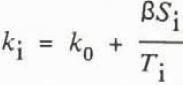
where β = 0.13Wm⁻¹ and S_i and T_i are the sea ice salinity in parts per thousand (ppt) and the temperature in °C. The thermal conductivity of pure ice k₀ ≈ 2.1 W m⁻¹deg⁻¹. The salinity was determined to within ±0.01 ppt (Wettlaufer and others, Reference Wettlaufer, Colony and Untersteiner1989). The measurement error associated with the conductive heat flux is ±0.1 Wm⁻² (ibid.,). This does not include the effect of brine drainage when the ice core is removed which is impossible to quantify in a systematic way.

Ice thickness measurements are taken at three locations within a 3.5 m² triangle around a temperature probe at each site. The average sampling interval was 6 days. Thickness changes can be measured to within ±0.1 cm (ibid.,) at each thickness gauge. The variance of growth rates among the three gauges at each site was computed for every sampling interval from which a mean standard deviation (over all sites) in growth rate of 0.2 cm d⁻¹ was determined. Taking an average latent heat over all sites of L = 2.95 × 10⁵ J kg⁻¹ and an average ice density of ρ = 900 kg m⁻³, the sampling error associated with the latent heat flux is 6.1 W m⁻². This error dominates the total sampling error.

The resulting fluxes were combined to compute the time series of F_w for all experimental sites. Unevenly spaced data (denoted by the dots in Figure 4) were interpolated to a regular time interval using a procedure similar to that of Akima (Reference Akima1978) (denoted by the dotted line in Figure 4). These interpolated data are then smoothed using a signal-plus-noise model whose results are plotted as a solid line in Figure 4. This procedure conserves the mean and the standard deviation of the data.

There are three “high flux” events during the time series. The maximum values of the smoothed curve for F_w are 37.0 W m⁻² on day 288, 27.0 W m⁻² on day 299, and 24.9 Wm⁻² on day 318. Because the oceanographic data recorded by other investigators are not yet available, we are unable to determine the source of the water associated with such large heat fluxes. The proximity of the drift to the Fram Strait leads us to believe that these events are associated with the mixing of warm Atlantic water into the mixed layer. This occurs either via entrainment caused by a substantial increase in the ice-ocean stress during a storm or via orographically induced intrusion caused by the proximity to the shelf break. Figure 5 gives a qualitative picture of the geographic location of the high flux events during the drift; the larger circle radii correspond to larger heat fluxes.

Fig. 4.

Observed oceanic heat flux during the CEAREX drift phase. The dots are the raw data, the dotted line is the result of a temporal interpolation, and the solid line is the result of a least squares fit to the interpolated data.

The question remains as to whether or not this method of measuring F_w yields reliable results. The reliability can be assessed only in terms of the consistency of these data with independent measurements. Such a comparison is made in Figure 6, where the solid line from Figure 4 (top) and the smoothed time series of the temperature of the mixed layer (Τ_w) 4 m below the ice bottom are plotted. The T_w time series is essentially a time series of the temperature gradient between the 4 m level and the ice bottom since equilibrium is maintained at the ice-ocean interface. Considering that the average freezing point of seawater in the Arctic Ocean is approximately −1.8°C, the departures from freezing occur over significant periods during the sampling interval. It should be noted that the maximum departure from the freezing point is only 0.12°C yet such a departure can have a significant effect on the ice morphology. The correlation between the two curves is 0.9. It is important to keep in mind that temperature departures alone do not constitute a large heat flux since the efficiency of the vertical transport of heat depends on the magnitude of the vertical current component as well. For example, the second peak in the T_w time series is broader than the first, yet the resultant heat flux is smaller. This is due to the higher velocities in the water column during the first event (McPhee, personal communication), which occurred as a result of a storm.

Fig. 5.

Drift trajectory from 19 September to 22 November 1988. The values of the oceanic heat flux, F_w , are superimposed where the circle radii increase with increasing magnitude. The inset shows the location of the drift with respect to the land masses of Greenland, Svalbard and Franz Josef Land moving west to east (left to right).

Fig. 6.

Time series of the oceanic heat flux and the mixed layer temperature, T_w, 4 m below the ice bottom. The top plot is the solid line from Figure 4, and the bottom plot is the average ocean temperature 4 m below the ice. Ocean temperature data supplied by McPhee (personal communication).

Conclusions

The role of the oceanic heat flux as a key constituent of the sea ice energy and mass balance is clear. The sensitivity of the ice to the magnitude of F_w and the dependence of ice-ocean models on the correct specification of F_w make it an effective tuning parameter in model studies. The horizontal variation of the component of F_w due to the heat loss of the warm Atlantic water is assumed to be negligible in most of the earlier model studies. This variation is taken into account in many interactive models yet the reality of such variations cannot be verified. The data presented here suggest that the assumption of horizontal homogeneity in F_w for regions close to the Fram Strait is ill-founded. The oceanic heat flux in this region of the eastern Arctic is time varying and may take on values that are an order of magnitude greater than the value of 2 or 3 W m ⁻² specified in most model studies. The virtual absence of F_w data is a major impediment to the validation of dynamic/thermodynamic ice models. The method described in this paper yields results that are accurate to within ±6.1 W m⁻² and are consistent with independent measurements in the water column. The observations show that F_w is independent of ice thickness.

However, the scatter in the data suggests that F_w does have some local variation. This may be the result of local variations in the turbulent structure of the oceanic boundary layer induced by under-ice topographic features. The scatter is in part due to the sampling error and in part due to under-ice topography; therefore, the sampling error in the latent heat flux of ±61. W m⁻² represents the net effect of both. Future studies will focus on distinguishing between these two effects and whether the topographic effect involves a coupling which is initiated by purely dynamic or both dynamic and thermodynamic effects. The time series is long for an experiment of this nature and covers an important part of the sea-ice thermal regime (fall freeze-up) in a geographical region close to the Fram Strait. We believe that this method provides valuable information and should be used in the future in both seasonal and perennial sea-ice zones. In order to construct an ample database we suggest that a number of unmanned buoy systems, similar to the design of Untersteiner and Thorndike (Reference Untersteiner and Thorndike1984), be deployed.

Acknowledgements

The authors thank D.R. Thomas and A.S. Thorndike for carefully reading the original manuscript and providing helpful comments. M.G. McPhee provided the ocean temperature data. The first author is associated with the Geophysics Program at the University of Washington. This research was supported by the Office of Naval Research, Arctic Sciences, contract N00014-87-K-0084, and by the Applied Physics Laboratory.