1 Introduction
Supervised machine learning methods have gained increasing attention in political science research (e.g., Beck, King, and Zeng Reference Beck, King and Zeng2000; Hill and Jones Reference Hill and Jones2014; Muchlinski et al. Reference Muchlinski, Siroky, He and Kocher2016; Cranmer and Desmarais Reference Cranmer and Desmarais2017) and specifically in connection to text analysis (e.g., Collingwood and Wilkerson Reference Collingwood and Wilkerson2012; Drutman and Hopkins Reference Drutman and Hopkins2013; Grimmer and Stewart Reference Grimmer and Stewart2013; Ceron et al. Reference Ceron, Curini, Iacus and Porro2014; Wilkerson, Smith, and Stramp Reference Wilkerson, Smith and Stramp2015; Workman Reference Workman2015; Wilkerson and Casas Reference Wilkerson and Casas2017). A core step in many research designs that involve text is the classification of documents into topical categories. Unsupervised topic models (Blei, Ng, and Jordan Reference Blei, Ng and Jordan2003; Grimmer Reference Grimmer2010; Roberts et al. Reference Roberts, Stewart, Tingley and Airoldi2013) have been arguably the goto method for political scientists for that purpose. In many contexts, supervised models would be more appropriate for the task at hand. However, supervised learning is costly because labeled data is required to train a classification model.
In this paper, we introduce active learning, a data labeling framework developed in computer science that can greatly increase the efficiency of data labeling (Settles Reference Settles2012). We concentrate on text data as a specific application, but active learning can be used with any kind of data in a supervised context. Much of the cost that comes from labeling texts is a result of sampling documents for an expert to label when classes are imbalanced. For example, a political scientist may wish to identify texts from a newspaper corpus that refer to a terrorist attack. Because terrorist attacks are rare events, we can expect that a random sample of newspaper articles will contain only a small number of articles about terrorist attacks, and an expert labeler will spend much of her time labeling irrelevant documents. In contrast, in active learning approaches, a learning algorithm suggests which observations the expert should label. With active learning, this suggestion is made according to a quantitative metric of the expected performance improvement that could be realized by each of the unlabeled observations in the data. Choosing data to be labeled in such a way reduces the labeling of documents that are not informative to the classification algorithm and thereby increases the efficiency of costly human labelers. We provide an introduction to the concept and an accessible starting point for political scientists who may benefit from this approach to labeling texts. We do not provide an exhaustive overview or theoretically rigorous exposition of the large number of varieties of active learning. For those who want to dive deeper into the theory and literature, see Settles (Reference Settles2012).
We conduct experiments that illustrate circumstances in which active learning produces the highest efficiency gains and show how common problems in social science—such as low intercoder reliability—may affect active learning.Footnote 1 We use three different text corpora and several classification models to compare active learning to the default approach to data labeling (random sampling or “passive learning”) and vary the amount of available training data. Our aim is not to adjudicate among various active learning algorithms but to show that various approaches all compare favorably to random sampling. We find that active learning approaches reduce the costs of supervised learning in many scenarios. Under realistic conditions, active learning can produce an eightfold decrease in the size of training data required to achieve the same performance as with passive learning. We find that in situations where the data are balanced—that is, the topic or class of interest makes up about half of the dataset—active learning provides no additional benefits. However, such balanced problems are relatively rare in political science (Ertekin et al. Reference Ertekin, Huang, Bottou and Giles2007; Sun, Wong, and Kamel Reference Sun, Wong and Kamel2009). For an additional contribution that, to our knowledge, is novel even to the computer science literature on the topic, we induce varying levels of intercoder (un)reliability. We find that even with fairly low intercoder agreement, active learning performs more efficiently than passive learning, even though both methods’ performance is reduced by labeling error (Mikhaylov, Laver, and Benoit Reference Mikhaylov, Laver and Benoit2012).
2 Approaches to Automated Text Analysis
We start by introducing the theoretical background and the variety of methods that fall under the umbrella of active learning.
2.1 Unsupervised vs. Supervised Learning
Automated text analysis methods can be categorized as supervised or unsupervised (Grimmer and Stewart Reference Grimmer and Stewart2013). Supervised models “learn” from a subset of data that is annotated by experts, while unsupervised models require no annotation but instead learn from correlations and co-occurrences of text features. While unsupervised models are important research tools, supervised models are usually a better choice for measuring topical categories the researcher has defined a priori. Conversely, unsupervised models are a better choice for discovering the latent topics within large corpora in the absence of a priori knowledge about the structure of these corpora.
When deciding between supervised and unsupervised models, it is important to consider the promises and pitfalls of each approach. Unsupervised models are good for summarization and exploration of large corpora. However, if the structure of the problem is well defined, that is, if there are specific topical categories defined by the researcher, supervised learning can be more useful than unsupervised strategies. Consider the example where a researcher is interested to find all social media posts related to a specific protest movement. In this case, the structure of the problem is well defined, that is, the researcher knows a priori what the classes of interest are (posts relevant to the movement and posts not relevant to the movement), and given a post, she would be able to determine the class membership of the said post. In contrast, an unsupervised method, such as a topic model, would not be guaranteed to produce a topic that is congruent with the protest movement class. Furthermore, if posts about this movement rarely occur in the data, it is unlikely that a single topic that captures this class emerges. The supervised method would, therefore, be the more natural choice in such a situation.
Furthermore, as previous research has shown, unsupervised methods often lack agreed-upon model selection procedures (Wallach et al. Reference Wallach, Murray, Salakhutdinov and Mimno2009), are highly unstable with respect to text preprocessing and hyperparameter choices (Wilkerson and Casas Reference Wilkerson and Casas2017; Denny and Spirling Reference Denny and Spirling2018), and require a great deal of human interpretation or post-hoc labeling (Chang et al. Reference Chang, Gerrish, Wang, Boyd-Graber and Blei2009). Conversely, model selection, hyperparameter/preprocessing choices, and model evaluation are all straightforward in supervised models.
Despite the many benefits of supervised approaches, their big disadvantage is the cost of labeling data—and this is likely a reason for the bigger popularity of topic models in political science (Quinn et al. Reference Quinn, Monroe, Colaresi, Crespin and Radev2010). Huge text corpora are very easily accessible to researchers (e.g., social media data, websites, legislative documents, etc.), but categorizing subsets of them into relevant and nonrelevant categories requires costly manual labeling.
2.2 Active vs. Passive Learning
In most supervised classification procedures, an expertFootnote 2 labels the class membership of a fixed set of observations in the data. These observations are usually a random sample drawn from the full dataset. Expert-labeled data are then used to “train” a learning algorithm to predict the labels of unlabeled observations in the dataset. We refer to this mode of data labeling and model training as “passive learning.” While this approach to classification works quite well in many cases, we see two situations in which the cost of labeling data “passively” can be prohibitively large:
-
(1) If the distribution of labels or classes in the corpus is imbalanced, that is, if one label occurs much more often than the other, it can take an enormous amount of labeled data to get enough information on the minority class for the algorithm to learn to recover it reliably.
-
(2) If there are many very similar documents, drawing data for labeling at random can be very inefficient (a lot of data is needed to learn representations of all relevant areas of the feature space).
If a concept appears in only 1 percent of documents, to get a sample of 20 relevant documents, an expert labeler would have to label, in expectation, 2000 documents. Even with this time-intensive labeling effort, a machine learning algorithm trained on only 20 observations is unlikely to perform well. Equivalently, if there are large clusters of very similar documents, then if documents are sampled randomly for labeling, the expert might spend a lot of time assigning labels to documents that are not informative to the classification algorithm because they differ so little in their features.
The computer science literature has consistently demonstrated that in these cases, active learning can be quite useful (see e.g., Schohn and Cohn Reference Schohn and Cohn2000; Tong and Koller Reference Tong and Koller2001; Roy and McCallum Reference Roy and McCallum2001; Dasgupta, Kalai, and Monteleoni Reference Dasgupta, Kalai and Monteleoni2005; Ertekin et al. Reference Ertekin, Huang, Bottou and Giles2007). In an active learning approach to classification, a learning algorithm suggests which observations the expert should label. This suggestion usually is made according to a quantitative metric of the expected performance improvement that could be realized by each of the unlabeled observations in the data. Documents are labeled in an iterative manner: after each iteration, a new classification model is trained and this model is queried for documents it is most uncertain about. This way, only documents that would actually help the algorithm to improve its performance are selected for labeling. In the next section, we explain each step of the active learning procedure in more detail.
3 Active Learning
3.1 General Principles of Active Learning
Given a set of documents with known labels
 $\mathbf{y}$
and a set of features (these can be bag-of-words features but also document metadata like timestamps or author information)
 $\mathbf{X}$
, the goal of text classification (or of machine learning in general) is to learn the function
 $y=f(\mathbf{X})$
that most accurately maps features to the labels beyond the specific set (training set)
 $\mathbf{y},\mathbf{X}$
(see, for example, Friedman, Hastie, and Tibshirani Reference Friedman, Hastie and Tibshirani2001, for an introduction). For simplicity of exposition, we concentrate on binary classification in this paper (i.e.,
 $y_{i}\in \{0,1\},\forall i$
), but all methods described here are applicable to multiclass classification (
 $y_{i}\in \{0,1,\ldots ,k\}\forall i$
) and continuous outcomes (see below).
There are many different implementations of the active learning framework. Each differs in what measure(s) are used to query unlabeled observations for an expert to label. Before discussing some of these variations in depth in Section 3.3, we give intuition on the logic of active learning using the least-complex variant, relying on logistic regression as the classification model and uncertainty sampling as the querying strategy (Lewis and Catlett Reference Lewis and Catlett1994).
We denote the set of unlabeled documents as
 ${\mathcal{U}}$
with all documents represented as
 $\mathbf{X}_{\boldsymbol{{\mathcal{U}}}}=\{\mathbf{x}_{i}|i=1,\ldots ,N\}$
, with
 $\mathbf{x}_{i}$
as a single document represented by a set of features (e.g., word counts or document metadata). Each document
 $\mathbf{x}_{i}$
has a corresponding true label
 $y_{i}\in \{0,1\}$
that can be obtained by asking an expert labeler to label it. We denote the logistic regression model as
 $f(\mathbf{x}_{i},\boldsymbol{\unicode[STIX]{x1D703}})=1/(1+e^{-\mathbf{x}\boldsymbol{\unicode[STIX]{x1D703}}})$
. The most basic active learning algorithm is then as follows:
-
(1) Start with an initial set
 ${\mathcal{L}}$
of documents
$\mathbf{X}_{\boldsymbol{{\mathcal{L}}}}$
with known labels
$\mathbf{y}_{\boldsymbol{{\mathcal{L}}}}$
-
(2) Train the model
$f(.,\boldsymbol{\unicode[STIX]{x1D703}})$
using the available training data
$\mathbf{y}_{\boldsymbol{{\mathcal{L}}}},\mathbf{X}_{{\mathcal{L}}}$
-
(3) Produce a predicted probability for each unknown document in unlabeled set
${\mathcal{U}}$
:
$\hat{\mathbf{y}}=f(\mathbf{X}_{\boldsymbol{{\mathcal{U}}}},\boldsymbol{\unicode[STIX]{x1D703}})$
-
(4) Use the query function to obtain a new document for labeling:
$z=q(\hat{\mathbf{y}})=\operatorname{argmin}_{i}|{\hat{y}}_{i}-0.5|$
-
(5) Obtain a label
$y_{z}$
for
$\mathbf{x}_{z}$
from the expert labeler -
(6) Add
$y_{z}$
and
$\mathbf{x}_{z}$
to
$\mathbf{y}_{\boldsymbol{{\mathcal{L}}}}$
and
$\mathbf{X}_{\boldsymbol{{\mathcal{L}}}}$
, remove
$\mathbf{x}_{z}$
from
$\mathbf{X}_{\boldsymbol{{\mathcal{U}}}}$
-
(7) Repeat Steps 2–6 until a stopping criterion is reached





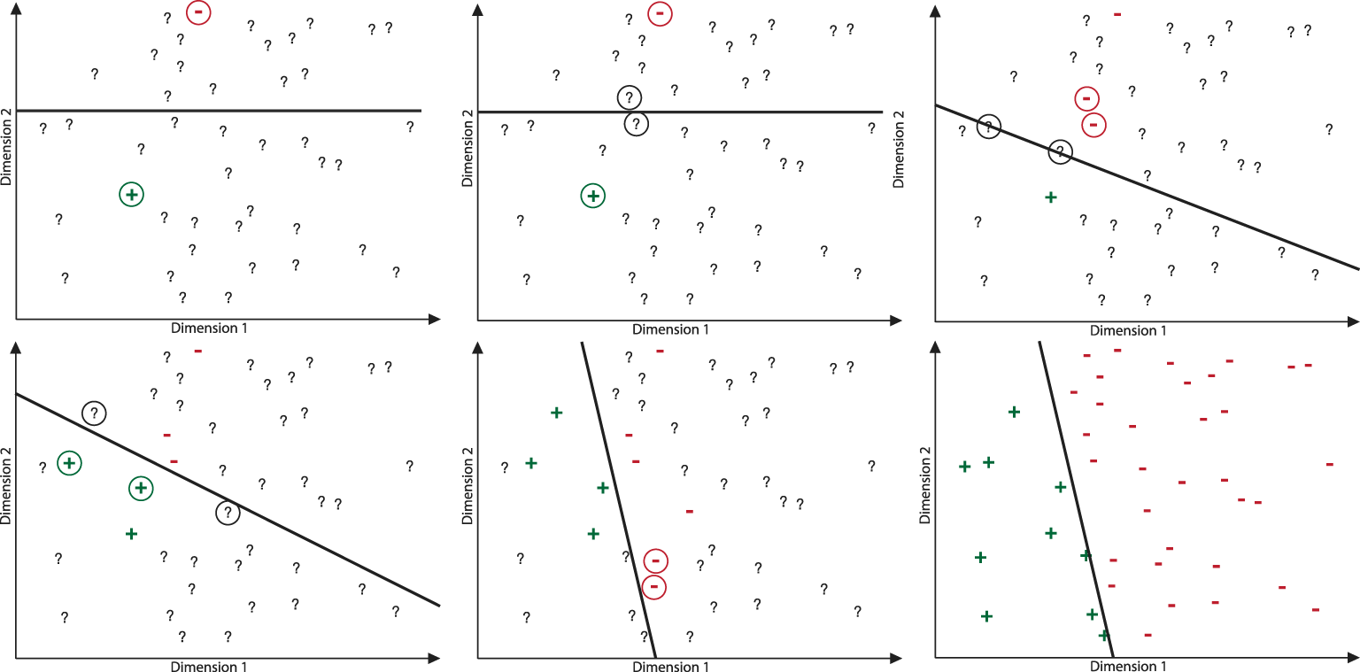
To summarize this algorithm: Starting with a population of documents, each of which is supposed to be classified, and an initial set of labeled data (this can be chosen at random or be produced from the domain knowledge of the researcher), a model is trained to separate the relevant from the nonrelevant documents. Each document of the population is then assigned a predicted probability from the model and the document with a probability closest to 0.5—that is, the document the model is least certain about—is selected for labeling. In many cases, it makes sense to select not a single document for labeling but the batch of least certain documents. The procedure is then repeated by retraining the model with the additional labeled data, querying more documents, labeling, etc. Usually the procedure is stopped when either the labeling budget is exhausted or a satisfactory classifier performance is reached (the definition of satisfactory, of course, depends on the application). Figure 1 displays a visualization of the algorithm. The bold line separating the observations in two-dimensional space corresponds to the 0.5 predicted probability threshold of the regression model. The active learning algorithm selects observations closest to this decision boundary in each iteration represented by each panel in the figure.
From left to right, top to bottom, the first five panels visualize the uncertainty sampling algorithm. Circles represent queries of unlabeled observations. Once an expert has labeled the data, they are represented by plus symbols for the positive class and minus symbols for the negative class. The last panel shows the true labels of all labeled observations.

The algorithm can be easily adapted for use with nominal outcomes of more than two categories or continuous outcomes. For multiclass classification, one way of accommodating such outcomes would be to select the new document using entropy as a measure of classifier uncertainty.Footnote 3 Given a classification model that produces predicted probabilities for each class an observation could fall in, the entropy over these predicted probabilities is a measure of uncertainty of the classifier about this observation. For the case of continuous outcomes, a measure of the variance of the predicted value can be used to assess classifier uncertainty.Footnote 4 To reiterate, these options for accommodating other outcomes are examples for the case of uncertainty sampling. For other query methods, slightly different approaches may need to be considered (see, for example, Körner and Wrobel Reference Körner and Wrobel2006; Settles Reference Settles2012, for more detailed guidance in such situations).
The strategy of actively selecting data to label intuitively reduces the number of labeled observations that are necessary to achieve a level of performance in the two situations described above. In the case of imbalanced classes, the model has initially little information about rare classes, given that the initial
 $\mathbf{y}$
most likely contains few observations belonging to the rare class. The model will be less certain about this class and therefore produces more samples for labeling from that class (this is assuming that there is some information about the class membership in the provided features
 $\mathbf{X}$
).
In the second case, where many documents in
 $\mathbf{X}_{{\mathcal{U}}}$
are very similar, intuition on the potential benefits can be gained from Step 3 in the algorithm above. Given three observations
 $\mathbf{x}_{1},\mathbf{x}_{2},\mathbf{x}_{3}$
with the distances, the feature space:
 $d(\mathbf{x}_{1},\mathbf{x}_{2})\ll d(\mathbf{x}_{1},\mathbf{x}_{3})\approx d(\mathbf{x}_{2},\mathbf{x}_{3})$
. If
 $\mathbf{x}_{1}$
is labeled, the model will produce a predicted probability closer to 0.5 for
 $\mathbf{x}_{3}$
as compared to
 $\mathbf{x}_{2}$
since it is very different from what the model has “seen” in previous iterations. Because
 $\mathbf{x}_{3}$
will provide more information than
 $\mathbf{x}_{2}$
, the expert labeler will be presented with
 $\mathbf{x}_{3}$
, thereby reducing inefficiency in the labeling.
3.2 Varieties of Active Learning
There is a large variety of ways to implement the active learning framework described in Section 3.1. Implementations can differ in several regards depending on the application: availability of unlabeled samples, the type of sample that is queried, the model and outcome, and the querying algorithm. These choices have produced a very large technical literature and make the choice for practical applications difficult. In this section, we will briefly describe the choices a researcher has, without going into technical depth (see Settles (Reference Settles2012), for an excellent in-depth review of the varieties of active learning).
Availability of Samples: Depending on the data source, documents for labeling may be available in different forms. In the procedure described in Section 3.1, there exists a pool of documents from which single documents can be selected for querying and classification (pool-based sampling). In other applications, not all documents are available at any time, but they are made available as a stream, for example, in stream-based APIs such as the Twitter Streaming API.Footnote 5 In this case, the active learning algorithm has to decide in real time which samples to select from the ones available at a certain time point (stream-based selective sampling) (e.g., Freund et al. Reference Freund, Seung, Shamir and Tishby1997). Finally, some authors have suggested producing a synthetic sample that is constructed in such a way that the model learns best from it after it was labeled (query synthesis) (Angluin Reference Angluin1988). This strategy can lead to multiple problems for text analysis in practice. Most importantly, a synthetically generated document will be difficult to label for an expert coder.
Model: In principle, any classification or regression model can be used in an active learning approach. Some querying methods have specific requirements for the model. For instance, the uncertainty sampling strategy used in Step 4 in the illustration above requires the model to produce a measure of uncertainty (e.g., a predicted probability) not just a discrete class prediction. There are also active learning varieties for quantitative outcomes. Uncertainty, in this case, is usually operationalized through the variance in the prediction of each unlabeled sample; so applications, in this case, are relatively straightforward.Footnote 6
3.3 Querying Strategies
How to measure the potential information gain for the model from an unlabeled instance is probably the component of active learning that received the largest amount of attention. Besides the uncertainty sampling querying strategy described in Section 3.1, there are a variety of methods to obtain unlabeled documents from the model. They can be roughly grouped into three groups (Settles Reference Settles2012): (1) algorithms that rely on the uncertainty of one or multiple classifiers about unlabeled samples (uncertainty based); (2) algorithms that are based on estimating the expected model performance, given a label was made available for unlabeled samples (model performance based); and (3) algorithms that exploit clustering or other structure in the data (structure based). The three most commonly used algorithms are margin sampling, query by committee, and expected model change. We review these in more detail. We refer the reader to the literature for more details on clustering approaches (see, for example, Settles (Reference Settles2012), for a more extensive review).
Margin sampling and uncertainty sampling are the algorithms most commonly used. We additionally discuss expected model change since it represents a different class of algorithms that are not focused on uncertain observations but rather try to optimize what the researcher might care about directly, the performance of the model. The details of how exactly we deploy these algorithms in our simulation studies are discussed in Section 4.2.
As is the case with other choices in machine learning such as the classification model or the method of tuning parameter optimization, it is difficult to make predictions about expected performance a priori, before interacting with the data.Footnote 7 It is, therefore, not possible to give direct guidance to researchers as to which of the querying algorithms is expected to perform best for the task at hand. This is the case because the function that is approximated by the classifier for text classification is highly complex, and the reasons for performance of various classifiers are not well understood. For practical applications, it is therefore recommended to explore the robustness of an active learning approach by also investigating the performance of several querying strategies.
However, there are other criteria besides robustness that applied researchers should consider when choosing a querying strategy. The various querying algorithms can vary drastically in their computational complexity and their ease of implementation. For instance, uncertainty sampling is a very simple approach that is easy to implement and computationally not very demanding. Predicting a label for each unlabeled observation is computationally much less demanding than, for example, estimating a new model for every unlabeled observation, as is the case for the expected model change algorithm. This can become quite expensive as the number of observations in a dataset increases. For the “query by committee” approach, it is necessary to train a committee of several classifiers, making this approach considerably more expensive than other approaches that require only a single model.
3.3.1 Margin Sampling
The algorithm used in Section 3.1 to demonstrate the fundamental principle of active learning is called uncertainty sampling. That is, the algorithm queries the observations for which it is most uncertain about their label. Logistic regression, however, might not be the model of choice for text classification. Support vector machines (SVM) is a very commonly applied model for text classification. The simple margin algorithm detailed in Tong and Koller (Reference Tong and Koller2001) is a special case of uncertainty sampling.Footnote 8 Essentially, the algorithm, similar to the logistic regression algorithm above, uses an uncertainty measure to query new observations for labeling by an expert labeler. Because the objective of the SVM model is to find a hyperplane that optimally separates classes in the feature space, observations that are closest to that hyperplane represent observations that the SVM is most uncertain of. For the simple margin classifier, at each iteration, an SVM model is trained and observations closest to the hyperplane are returned to an expert for labeling (as visualized in Figure 1 for the two-dimensional case).
3.3.2 Query by Committee
The query by committee approach follows principles similar to the uncertainty sampling strategy. However, instead of relying on the uncertainty of a single model, uncertainty is measured using disagreements in classification decisions among a committee of models (Seung, Opper, and Sompolinsky Reference Seung, Opper and Sompolinsky1992).
For the query by committee approach to active learning, a committee of models,
 ${\mathcal{C}}=\{\unicode[STIX]{x1D703}^{(1)},\ldots ,\unicode[STIX]{x1D703}^{(C)}\}$
, is trained on the current labeled set
 ${\mathcal{L}}$
. Each classifier in this committee represents a different hypothesis for how the version spaceFootnote
9
should be partitioned. Classifiers in the committee make predictions for each of the documents in the unlabeled set
 ${\mathcal{U}}$
. The
 $m$
documents where the committee disagrees the most are returned to the expert to label. This disagreement is usually computed using vote entropyFootnote
10
or Kullback–Leibler divergence (Kullback and Leibler Reference Kullback and Leibler1951).
In the original formulation, Seung, Opper, and Sompolinsky (Reference Seung, Opper and Sompolinsky1992) use perceptron learners, but there is no clear agreement on how to best choose a set of models for the committee. Some formulations of query by committee make use of ensemble methods such as bagging (Freund and Schapire Reference Freund and Schapire1997) and boosting (Abe and Mamitsuka Reference Abe and Mamitsuka1998) to form committees. Others choose a diverse set of ensemble classifiers (Melville and Mooney Reference Melville and Mooney2004). In a review of the literature, Settles (Reference Settles2012) suggests that there is no clear guideline for size and model choice. The committee only needs to satisfy two conditions: (1) models in the committee must represent different regions of the version space; (2) there must be some disagreement among committee members.
3.3.3 Expected Model Change
While margin sampling and query by committee select unlabeled observations based on an uncertainty measure, another class of active learning approaches seeks to quantify the potential informational gain of each candidate unlabeled observation. These methods query the unlabeled observations that would result in the greatest change to the current model (expected model change), the greatest reduction of generalization error (expected error reduction), or the greatest reduction in output variance (variance reduction), if we knew its label (Settles Reference Settles2012; Roy and McCallum Reference Roy and McCallum2001). These approaches are computationally expensive as they require that a model be fit for each candidate observation in the unlabeled set. For text classification problems, it is common that the set of unlabeled observations is quite large, a potential drawback of this approach (Settles and Craven Reference Settles and Craven2008).
The expected model change approach as originally formulated by Settles, Craven, and Ray (Reference Settles, Craven and Ray2008) selects unlabeled observations with the largest expected gradient length, the average length of the gradient of the loss function
 $\ell _{\unicode[STIX]{x1D703}}$
obtained by adding the training tuple
 $\langle x,{\hat{y}}\rangle$
, predictors
 $x$
from the unlabeled set
 ${\mathcal{U}}$
and
 ${\hat{y}}$
, and the expected label, given the current model to labeled set
 ${\mathcal{L}}$
. Unlabeled observations are queried according to
 $\text{argmax}_{x}\,P_{\unicode[STIX]{x1D703}}(y_{i}|x)\Vert \unicode[STIX]{x1D6FB}\ell _{\unicode[STIX]{x1D703}}({\mathcal{L}}\cup \langle x,{\hat{y}}\rangle )\Vert$
. This essentially chooses the unlabeled observations that, if labeled, would maximally change the output of the model. Other slight variants of this approach have proven effective in many domains (Freytag, Rodner, and Denzler Reference Freytag, Rodner and Denzler2014).
3.4 Biased Training Data, Generalization Error, and Intercoder Reliability
The fundamental principle of active learning is to produce training datasets that are biased to include documents that the classification model is uncertain about. That is, the dataset used to train the classification model is not representative of the total corpus. This can have consequences for several aspects of the coding process.
Estimates of generalization error (i.e., how well the classification model will perform on the general corpus) obtained from the training data can be biased or inconsistent estimates of the true generalization error. While we cannot claim to know the direction of bias in generalization error estimates in all circumstances, it has been established that it is a biased estimate in an active learning setting (Baram, Yaniv, and Luz Reference Baram, Yaniv and Luz2004). If precise estimates of generalization error are required or a choice between multiple active learning methods based on unbiased estimates of generalization error is desired, part of the labeling budget has to be spent on labeling data that has been selected randomly (Ali, Caruana, and Kapoor Reference Ali, Caruana and Kapoor2014). In our simulation study, we explore the gravity of this problem by comparing estimates of generalization error obtained from labeled data that was actively sampled with unbiased estimates.
Expert labelers are most likely presented with cases that are more difficult to label. This is a problem that has been, to our knowledge, omitted from the computer science literature.Footnote 11 This could, in turn, lead to the complication that the error rate of the expert labelers is likely to be higher as compared to randomly selected labeled data. An additional point to consider is that estimates of intercoder reliability, analogous to the generalization error, cannot be extrapolated to the general corpus. In simulations described in detail below, we simulate varying levels of intercoder reliability to investigate to what extent labeling error influences the performance of active learning and random sampling approaches.
4 Simulation Study
To investigate the performance, efficiency, and practical applicability of active learning, we conduct a simulation study on three selected text datasets, varying query strategy, class balance, and inducing error in the labeling process (intercoder reliability). In this section, we detail our data, simulation design, and implementation.
4.1 Data
We use three corpora that vary by text length and text style. By varying the text domain, we hope to demonstrate that active learning works across many of the domains relevant to political scientists. We use a corpus of tweets, a corpus of Wikipedia talk page entries, and a corpus of news articles from the news website Breitbart. These corpora vary in document size from small, to medium, to large, respectively. The style of writing in each also varies, with social media, specialized/academic writing, and news articles, respectively.
-
(1) Twitter: This corpus is composed of 24,420 tweets collected from a random sample of German Twitter users. The sample of tweets is a subset of a larger random sample of all tweets authored by about 80,000 users. Each tweet was labeled as being about the refugee topic or not by German-speaking CrowdFlower workers. Of the 24,000 tweets, about 700 are labeled as being about the topic. The dataset is used by Linder (Reference Linder2017) to study public reactions to refugee allocation in the German refugee crisis.
-
(2) Wikipedia: This corpus of 159,571 Wikipedia talk page comments includes annotations of different kinds of toxic comments. The database was released as part of a machine learning competition, “Toxic Comment Classification Challenge” on the website Kaggle that is sponsored by ConversationAI, a team organized by Jigsaw and Google to build “tools to help improve online conversation.” The goal of this competition is to classify the types of toxic comments using the provided expert annotations. For our simulations, we chose the label “toxic” because it has the most support of all represented classes. “Toxic” comments are aggressive comments, violent comments, personal attacks, etc. that do not contribute to a healthy and productive discussion on talk pages.
-
(3) Breitbart: This corpus of 174,847 news articles represents the population of articles on the Breitbart news website. These articles each come with meta tags that are chosen by Breitbart authors and editors. For this dataset, we use the label “Muslim identity,” which indicates whether a specific reference to Muslim identity was made in the article tags. This corpus is used to measure how moral and emotional frames in news media can increase support for violence against outgroups in Javed and Miller (Reference Javed and Miller2018). To make the simulations computationally more feasible we randomly sampled a subset of 25,000 articles for this study.
Even though we use datasets that realistically reflect data that are used in political science research, we must point out that data in a simulation study can never be a representative basis on which to make with certainty general statements about the performance of different machine learning algorithms on other tasks or in other data. Due to the many combinations of possible data features, the differences in structure of corpora, the diversity in research objectives, and the varying degrees of flexibility of statistical learning algorithms, it is impossible to generalize reliably from a handful of datasets.
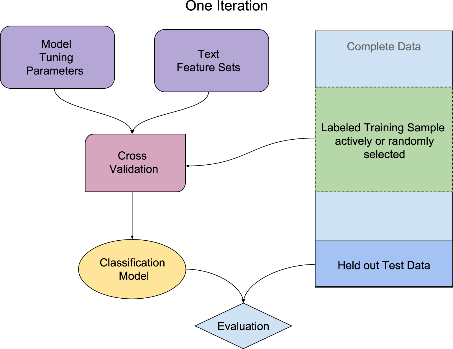
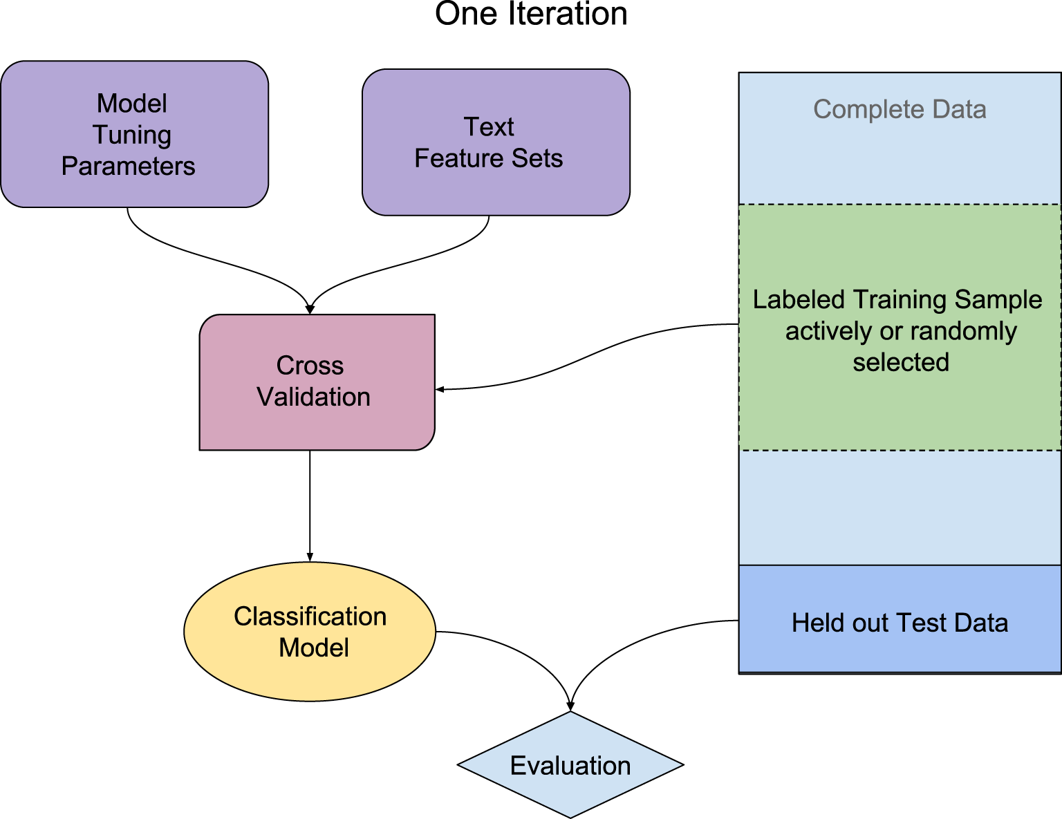
Design of the simulation study. In each iteration of the algorithm model tuning parameters and text feature sets are selected via cross-validation on the training data available from previous iterations. The best performing classification model is then evaluated on a held-out test dataset.
4.2 Design and Implementation
We conduct two simulation studies. The first study compares the performance of active learning with three different querying strategies to passive learning on the datasets described above. In the second simulation study, we investigate whether and how error in the labeling process affects active and passive learning differentially.
Each study simulates the data labeling process in an iterative manner. At each iteration a batch of documents is selected—using the querying algorithm for active learning or random sampling for passive learning—and added to the training data available to the classifier at that iteration. We draw 20 documents at each iteration and stop once we have processed 25% of documents in the corpus or all positive samples are labeled. We refer to one labeling process completed in this manner as a run. In most cases we repeat each run 50 times in order to obtain Monte Carlo estimates of the performance statistics of the various algorithms.Footnote 12
Figure 2 illustrates the design of a single iteration of the simulation. Before each run, the data are randomly split up into a dataset that is available for labeling and training and a held-out test set. The data that are available for training at each iteration are used to train a SVM classification model which is evaluated at each iteration on the held-out test set.
In addition to training the classifier at each iteration, a model and feature selection step is conducted. Using fivefold cross-validation and randomized parameter search (Bergstra and Bengio Reference Bergstra and Bengio2012), the tuning parameters of the SVM as well as the best feature set are selected at each step.Footnote 13
In order to demonstrate the performance of the various algorithms under realistic conditions, we artificially induce various degrees of class imbalance into the datasets. We create new datasets with different levels of class imbalance by oversampling and undersampling the positive class from the original corpora. We use the following positive class proportions: 0.01, 0.05, 0.10, and 0.50.
We compare four algorithms for selecting documents to label: active learning with margin sampling, active learning with query by committee, active learning with expected model change and randomly sampled labeled data. See Section 1.6 in the Supplementary Appendix for the details of how we implemented various querying strategies. At each iteration after having selected the next 20 training instances we train the same SVM model for the final evaluation. We chose this procedure to compare the quality of the selection of training data while keeping the classification algorithm constant rather than confounding it with the performance of the classification model. For the query by committee algorithm, however, this means that a different model is used in the final classification step than in the querying step (margin sampling and expected model change are both based on SVMs in our implementation). This means that the query by committee algorithm might potentially perform better if the query algorithm and classifier for evaluation would match. This design does allow us to investigate whether the active learning algorithm is still providing benefits to the researchers, even when a different final classification model is used with the training data obtained. Having to “lock in” one specific classifier for a project might be a significant disincentive to using active learning, therefore assessing whether an actively sampled set of training data is superior to a randomly sampled one independently of the classification model is an important question for the practical applicability of the method.Footnote 14
In addition to the main simulation study, we conduct an additional study, exclusively on the Twitter data, to test how varying levels of intercoder reliability can affect the performance of active learning approaches. We induce random error in labeling assignment in the training data while leaving the held-out data used to evaluate performance unchanged, simulating coder error. We simulate varying levels of intercoder reliability using the following algorithm:
For each level of intercoder reliability
 $a_{i}\in \{0.7,0.8,0.9,0.95\}$
:
-
(1) For each label
$y_{j}$
in the training set
$\mathbf{y}$
, generate a uniform random number
$u_{j}\in [0,1]$
-
(2) If
$u_{j}\geqslant a_{i}$
, flip the label
$y_{j}$
from 1 to 0 or vice versa (
$y_{j}^{\prime }=|y_{j}-1|$
) resulting in transformed labels
$\mathbf{y}^{\prime }$
-
(3) Sample observations to “label” using the maximal margin sampling algorithm with input
$\mathbf{y}^{\prime }$
and corresponding feature set
$\mathbf{X}$


For the intercoder reliability simulations we apply the margin sampling algorithm as well as the query by committee algorithm in order to evaluate if they could be affected differentially by the introduced noise.
4.3 Results
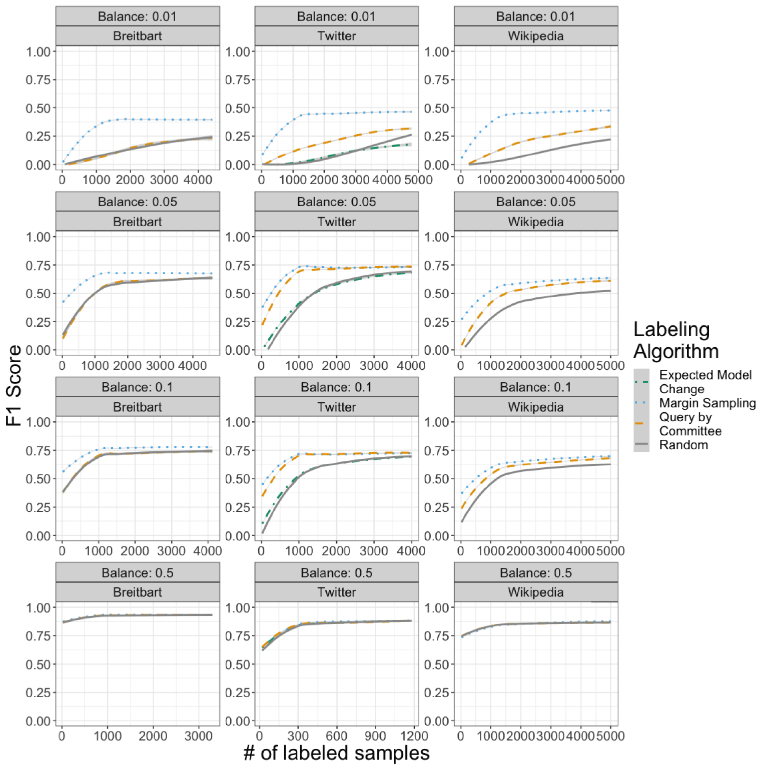
Figure 3 displays the classification performance on the held-out test set for all three datasets for the first simulation study (no error in the labeling process). Each row of Figure 3 represents a level of class imbalance. “Balance: 0.01” means that there are 1% relevant labels and 99% nonrelevant labels. In the columns are the three different datasets. The lines in the plots are generalized additive model fits across replications of the same conditions. The different lines show the classifier performance for the several labeling algorithms, that is, active learning with the margin, query by committee and expected model change algorithms and passive learning with randomly selected training data. All Figures display the performance of the model (defined as the F1-scoreFootnote 15 ) for different amounts of available training data (ranging from 20 documents to 5000 documents). Note that there are different amounts of training data in the different balance levels. This is due to the fact that, for example, for a balance of 0.5, the total dataset size is constrained to two times the number of relevant documents in the corpus. The original Twitter data, for example, has about 3% relevant tweets, which means that creating a balanced dataset reduces the total size of the data considerably.
F1-score for experiments. The panel columns correspond to the datasets and the rows to the different levels of class imbalance. Dots represent single replications of the experiment and smoothed lines are fits (and standard errors) of a generalized additive model.
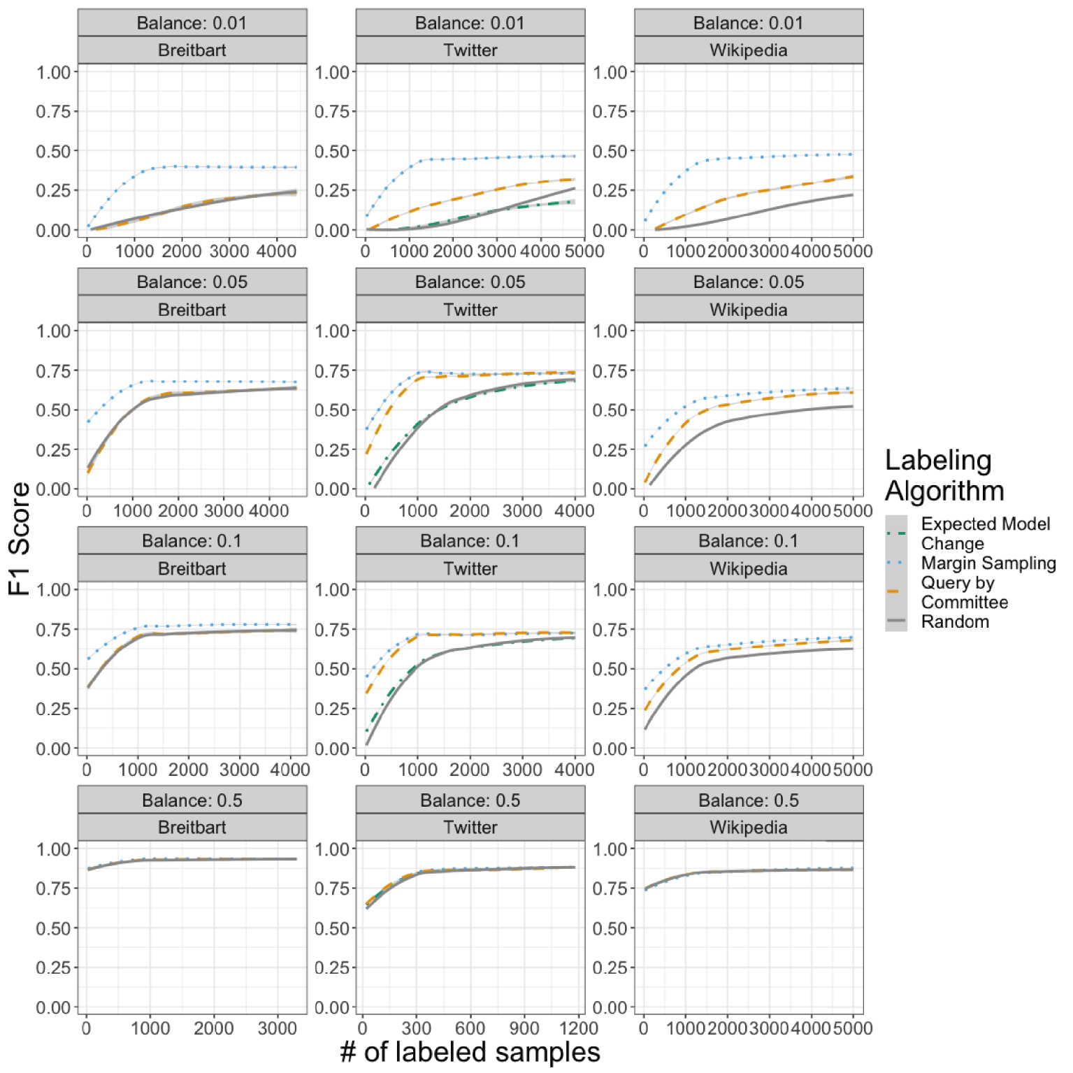
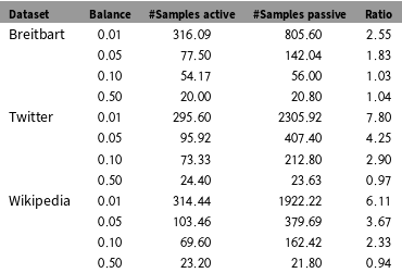
The gains in performance and reduction in cost resulting from the active learning approach are clearly visible in the imbalanced conditions. The model trained on the randomly labeled data often does not achieve the same performance as the active learning models, even with a quarter of the total corpus being labeled.Footnote 16 The best active learning algorithms reach their best performance very quickly with little increase in performance when adding additional training data. To quantify the gains achieved through active learning, Table 1 displays the average number of training samples that are required to achieve an F1-score of 0.1 for active learning with the margin algorithm and passive learning, as well as the ratio of the two. Depending on the balance of the data and the dataset, passive learning requires the same amount of data (balanced data Wikipedia) or up to almost eight times the amount of training data (Twitter data with 1% relevant documents). The relationship of the performance differential with the balance of the data is striking. With 1% of the data being relevant, the difference is dramatic, while for the balanced data, there is virtually no difference in performance.
Number of training samples required to reach an F1-score of 0.1 for active and passive learning.

We also observe significant differences between the various querying algorithms. Across all datasets and balance conditions, the margin algorithm performs best followed by query by committee and expected model change. Expected model change seems to produce no added performance compared to randomly annotated data. These results demonstrate that the choice of query algorithm can significantly impact the performance a researcher can expect from their classifier. As discussed in the theoretical sections, as is the case in many machine learning applications, it is difficult to choose a priori which algorithm will perform best for a given problem. In this sense, the results of the different querying algorithms from this simulation study should not be interpreted as guarantees that generalize for any other application in text classification but, rather, as a demonstration that the choice of querying algorithm can matter and researchers should consider experimenting with different algorithms. Furthermore, the query by committee algorithm had the disadvantage of the mismatch of classifier that was used to evaluate and the model involved in the query step.
The length and style of the documents seem to matter as well. The difference between the active and random labeling strategies is less evident for the Breitbart corpus than for the other two. The Twitter corpus, which is composed of the shortest documents, shows the largest differences.
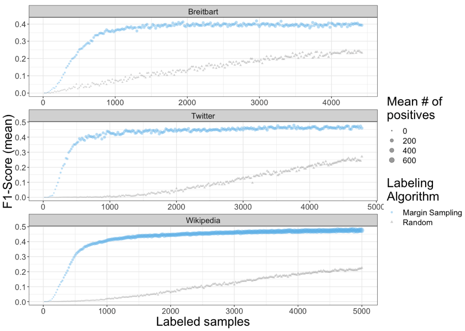
Performance by number of labeled examples for classifiers trained with active and passive learning (with class balance 0.01). Dots represent the average classifier performance across replications. Dot size is proportional to the average number of positively labeled observations in the training sample across replications.

To illuminate further why the active learner performs so much better in the imbalanced conditions, we zoom in on the 1% relevant data condition and additionally display the number of positive (or minority class) documents in the training data. These results are displayed in Figure 4. In this figure, each dot represents the average F1-score across experimental replications. The size of the dots represents the average number of positively labeled documents in the training data. The following pattern can be observed: the active learning algorithm acquires positively labeled documents (i.e., documents belonging to the minority) much faster than the passive algorithm. While the proportion of positive sample increases linearly—proportionally increasing with the size of the training data—for the passive algorithm, the active learner acquires almost all its positive samples within the first 1000 training data samples. This explains the performance difference: the active learner has much more information on the minority class much earlier, allowing it to perform better more quickly. This is additionally evident when inspecting precision and recall separately (see Figures 1 and 2 in the Supplementary Appendix). The availability of a more balanced training set (i.e., more observations of the minority class) leads to drastically improved recall which in turn is pushing the F1-score which is composed of precision and recall.
The better performance of active learning is mostly driven by this increased recall. In some instances when precision is higher for active learning than for random annotation, the results are mixed. In some cases in our simulations, the active learning algorithms produce even lower precision. The slightly reduced precision may be a result of the same mechanism: in situations where classes are very imbalanced, high precision and low recall can result from predicting the majority class for most observations. Therefore, as the classifier gains more information on both classes, false positives become more likely, reducing the overall precision. The reduction in precision is minor, however, and dwarfed by the increase in recall. For researchers that, for some reason, specifically want to improve precision, this could be a concern.Footnote 17
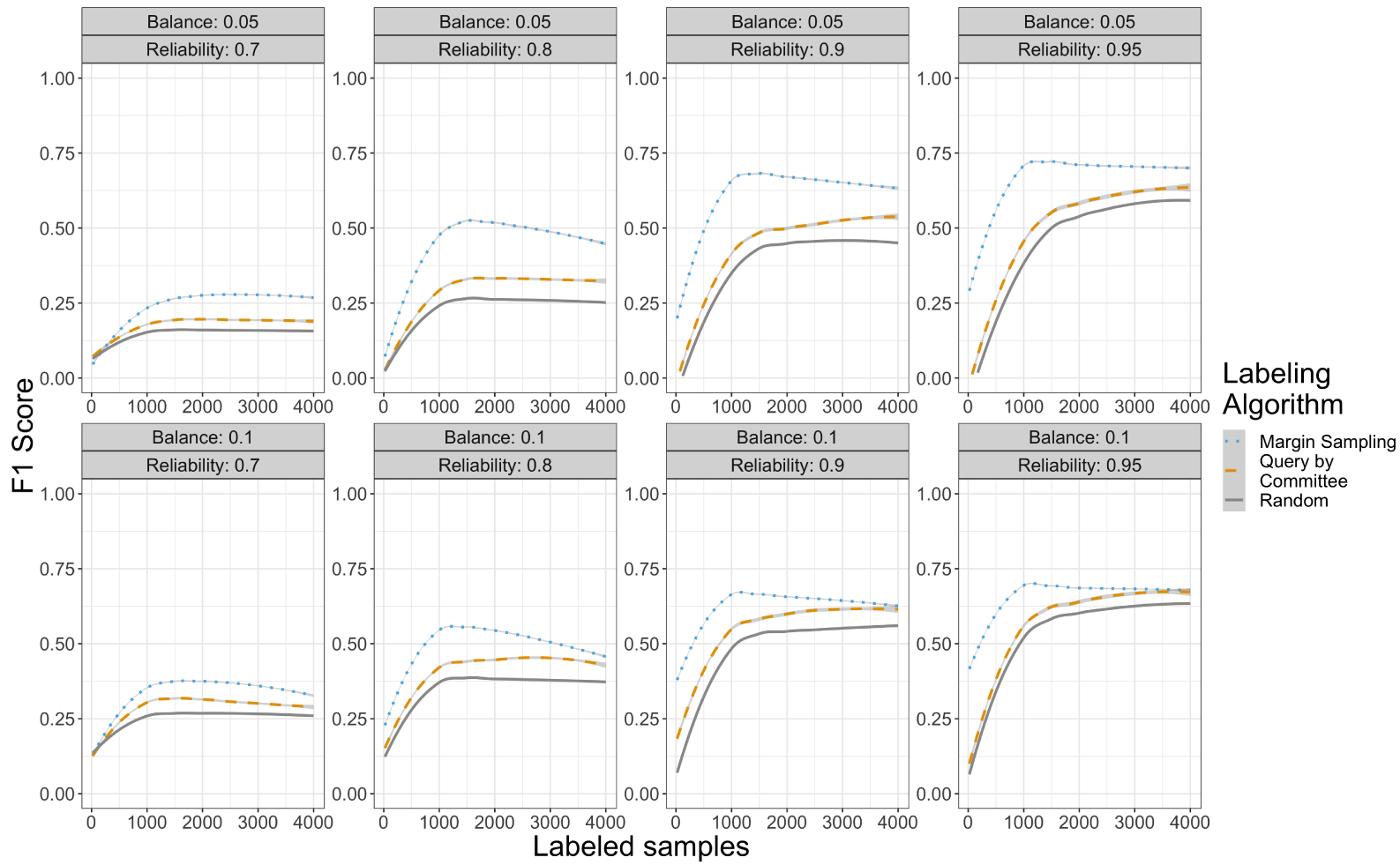
Active learning and passive learning performance on the Twitter dataset with different levels of simulated intercoder reliability.

Figure 5 displays the intercoder reliability results that were obtained by running the experiment with varying probability of error in the label assignment for the imbalanced condition (0.01) on the Twitter data. As expected, the overall performance of the classifier is affected by the amount of noise introduced into the training data by the simulated low coder reliability. Active learning outperforms random sampling even when the assignment of labels to the data is noisy. This holds for both the query by committee and margin algorithms. The margin algorithm seems to be affected more by additional samples added to the training data after the initial one to two hundred. We speculate that this has to do with the balance in the available training data. As shown above in Figure 4, the algorithm gets most of the minority class samples early (i.e., within the first 1000 labeled observations). Therefore, most of the additional labeled samples added to the training later are from the majority class and most labels for the minority class are results of the error process. That is, errors that are introduced in this later data affect only one class. This increase in false positives leads to a relatively significant decline in precision (see Figure 3 in the Supplementary Appendix). The query by committee algorithm seems less susceptible to this decrease in precision even though not immune.
Comparison of generalization error (in terms of F1-score) in training and test set for active learning with margin querying strategy. Results are from the Twitter dataset.

In Figure 6, we explore the topic of generalization error further. Each panel mirrors the panels in Figure 3. Since we are discussing the results in terms of error, the
 $y$
-axis displays 1 minus the F1-score. The red dashed line is the performance of the margin algorithm on the held-out sample and is identical to the corresponding line in Figure 3. The blue line displays the average of the average F1-scores obtained from cross-validating the model on the available labeled data. That is, the blue line represents the estimate of the generalization error as it would be available to a researcher that does not have an unbiased ground-truth test set, whereas the red line represents the true generalization error. We emphasize that, above, we established that active learning outperforms random sampling of the training data. In this section, we only discuss the estimation of generalization error to the population of samples. The results in Figure 6 demonstrate that the estimated generalization error in the labeled dataset is indeed different from the unbiased estimate. In the more balanced conditions, the error estimated from the labeled data tends to overestimate the error, whereas in the imbalanced conditions, it tends to underestimate the error.
The lack of a precise estimate of generalization error is a disadvantage that has to be weighed against the improved performance of active learning. We expect that in most cases, improved performance would be valued higher than confidence about the exact performance. But if a precise estimate of generalization error is required, we recommend that researchers use part of their labeling budget to label randomly selected samples. This portion of the data can then be used to estimate this error.
There may be concern that the hyperplane fit in each iteration of the margin algorithm might get stuck in a suboptimal version space. To investigate this, we ran simulations varying the percent of each batch that is sampled randomly: 25%, 50%, or 75% of documents were sampled randomly and the remaining sampled from proximity to the hyperplane. Including some purely random selection allows more exploration of the feature space and prevents the active learner from restricting its queries to a submanifold of our feature space. Performance was about the same across conditions, which suggests that, at least in the Twitter data, trapping suboptimal submanifolds are not a large concern.Footnote 18 Additionally, these simulations demonstrate that much of the gain in classifier performance is coming from the few observations in each batch that are closest to the hyperplane: decreasing the batch size may increase the efficiency of active learning if it is computationally feasible to do so.
5 Discussion
In this paper, we introduce the active learning paradigm and illustrate when it can be useful for labeling texts. We conduct several simulations with three datasets, varying the class balance, document length, and sample type. We find that the active learning approach—when compared to random sampling—reduces the costs of supervised learning in many realistic scenarios. Much of the extra cost with random sampling is due to the random approach’s inefficient selection of documents to label when classes are imbalanced. Random sampling can produce very imbalanced training data that have too much information on some part of the feature space and not enough on others. For imbalanced datasets, we find that passive learning methods can require up to eight times as much training data to achieve the same performance as active learning. We also find that these results hold even in the presence of noise in the labeling process. The results, especially with regard to the balance of the dataset, confirm theoretical expectations that the active learning algorithms help to reduce inefficiency in labeling. We also demonstrate that the choice of querying method can affect the amount of labels required to achieve a specific level of classification performance. Given that general statements about the potential performance of different querying algorithms are difficult to make, we recommend that researchers experiment with different methods. Overall, active learning produces a biased training dataset that produces classification results that are better or at least as good as random sampling on out-of-sample data.
This bias in the training set, however, leads to some potential limitations that applied researchers should be aware of: relying solely on the actively sampled training data prohibits accurate estimation of the true generalization performance of the model. This can be a major concern in academic settings, where the error rate of the machine learning model is relevant to the confidence in substantive results that are based on the predictions of the said model. However, this problem can easily be circumvented by dedicating a small amount of the labeling budget to a held-out random sample that is exclusively used to estimate out-of-sample performance.
Not knowing the true performance of the model complicates model selection as well. If no randomly sampled data are available, the model cannot be optimized for prediction on out-of-sample data. Furthermore, it is unknown whether the training data that were selected through active learning are optimal for other classification models as well. This may lead to concerns that the researcher has to commit to a specific classification model already at the labeling stage of the research project. It is important to note, however, that the evaluations in our simulation study were done on a randomly selected held-out dataset. That is, given our results and a large literature in computer science, applied researchers can expect that the active learning model performs better or at least as good as that in practice, even if additional effort would be required to obtain an unbiased estimate of the performance. Regarding the second concern about “lock-in” on a specific model, our results on query by committee suggest that active learning methods can outperform random sampling even in situations where a different final learning model is used with the training data.
It should be noted that the limitations that apply to “classical” machine learning for text classification apply to active learning as well. For instance, a classifier can only be as good as the training data it is based on. In cases where the language pertaining to the relevant class of documents changes (concept drift), the performance of the classifier can decrease drastically if applied to data from different time points. Furthermore, the classification methods that are used should be appropriate to the data at hand. For instance, if the data has known dependency structures like clusters or time-series structure, more appropriate classification algorithms might be used that do not assume a collection of independent observations.
A concern specific to active learning is that there may be an interaction between structure in the data and the dependence in samples. That is, in a case where the initial set of labeled data is an odd sample that only contains documents from one time period or cluster, could it happen that the model is led astray by this structure and never obtains data that is informative for other clusters? The results for the data in our experiments alleviate this concern. No guarantees can be made that generalize for all applications, but one can argue that active learning is a priori better suited to explore the relevant sections of the data. For instance, if the initial sample is from a specific cluster or time period in the data, the active learner may be more likely to explore other clusters in the data because the observations there are different from the observations in the “known” cluster, and, therefore, the model is less certain about them.Footnote 19
Our results demonstrate that in many scenarios, active learning can provide large efficiency gains for supervised text analysis methods in political science (or machine learning applications in general). These efficiency gains are most dramatic when classes are highly imbalanced. Having imperfect coder reliability does not eliminate the efficiency advantage that active learning has over random sampling. We hope our findings will serve to promote the use of supervised learning approaches for automated text analysis by making the process less costly and less time-intensive for researchers.
Acknowledgements
Work supported by NSF award SES 1523355.
Data Availability Statement
Replication materials are available as Miller, Linder, and Mebane (Reference Miller, Linder and Mebane2019).
Supplementary material
For supplementary material accompanying this paper, please visit https://doi.org/10.1017/pan.2020.4.