2.1 Spectral densities of plasma density fluctuations in collisionless multicomponent plasmas

The Klimontovich equation describes the temporal evolution of the microscopic phase-space densities or exact distribution functions $f_{\boldsymbol{p}}^{{\it\alpha}}(\boldsymbol{r},t)$ (Klimontovich Reference Klimontovich1967). In weakly coupled plasma systems, temporal and spatial considerations point towards the conceptual decomposition of $f_{\boldsymbol{p}}^{{\it\alpha}}(\boldsymbol{r},t)$ into an ensemble-averaged continuous component ${\it\Phi}_{\boldsymbol{p}}^{{\it\alpha}}$ and a fluctuating component ${\it\delta}f_{\boldsymbol{p}}^{{\it\alpha}}(\boldsymbol{r},t)$ , $f_{\boldsymbol{p}}^{{\it\alpha}}(\boldsymbol{r},t)={\it\Phi}_{\boldsymbol{p}}^{{\it\alpha}}+{\it\delta}f_{\boldsymbol{p}}^{{\it\alpha}}(\boldsymbol{r},t)$ . From the general properties of the resulting equations, a mathematical decomposition of the fluctuating component also into two constituents arises, i.e. ${\it\delta}f_{\boldsymbol{p}}^{{\it\alpha}}(\boldsymbol{r},t)={\it\delta}f_{\boldsymbol{p}}^{{\it\alpha},(0)}(\boldsymbol{r},t)+{\it\delta}f_{\boldsymbol{p}}^{{\it\alpha},\mathit{(ind)}}(\boldsymbol{r},t)$ , where the natural part ${\it\delta}f_{\boldsymbol{p}}^{{\it\alpha},(0)}(\boldsymbol{r},t)$ is triggered solely by particle discreteness and corresponds to a fictitious system with the interactions between particles being switched off and where the induced part ${\it\delta}f_{\boldsymbol{p}}^{{\it\alpha},\mathit{(ind)}}(\boldsymbol{r},t)$ is triggered by the interaction of the fluctuating fields with the discrete particles (Tsytovich Reference Tsytovich1989, Reference Tsytovich1995). By employing the definition of natural fluctuations, a closed form relation can be found for the ensemble average of the product of two natural fluctuating components of the microscopic phase-space density at different time instants and different positions (Ichimaru & Yakimenko Reference Ichimaru and Yakimenko1973; Yakimenko & Zagorodny Reference Yakimenko and Zagorodny1974; Tolias et al. Reference Tolias, Ratynskaia, Panarese, Longo and de Angelis2015). In the absence of external electromagnetic fields, its space–time Fourier transform, also known as the natural correlator, is given by Tsytovich (Reference Tsytovich1989, Reference Tsytovich1995), Tolias et al. (Reference Tolias, Ratynskaia, Panarese, Longo and de Angelis2015)

(2.1) $$\begin{eqnarray}\langle {\it\delta}f_{\boldsymbol{p},\boldsymbol{k},{\it\omega}}^{{\it\alpha},(0)}{\it\delta}f_{\boldsymbol{ p}^{\prime },\boldsymbol{k}^{\prime },{\it\omega}^{\prime }}^{{\it\beta},(0)}\rangle =\frac{1}{(2{\rm\pi})^{3}}{\it\delta}_{{\it\alpha}{\it\beta}}{\it\delta}(\,\boldsymbol{p}-\boldsymbol{p}^{\prime }){\it\delta}({\it\omega}+{\it\omega}^{\prime }){\it\delta}(\boldsymbol{k}+\boldsymbol{k}^{\prime }){\it\delta}({\it\omega}-\boldsymbol{k}\boldsymbol{\cdot }\boldsymbol{v}){\it\Phi}_{\boldsymbol{ p}}^{{\it\alpha}}.\end{eqnarray}$$

Application of these decompositions to the Klimontovich–Poisson system (for velocities much less than the speed of light, magnetic field generation by the particles is negligible) together with separating spatio-temporal scales, neglecting high-order fluctuations, ensemble averaging and Fourier transforming, leads to the fluctuation equation

(2.2) $$\begin{eqnarray}{\it\delta}f_{\boldsymbol{p},\boldsymbol{k},{\it\omega}}^{{\it\alpha}}={\it\delta}f_{\boldsymbol{ p},\boldsymbol{k},{\it\omega}}^{{\it\alpha},(0)}-\frac{4{\rm\pi}e_{{\it\alpha}}}{k^{2}{\it\epsilon}_{\boldsymbol{k},{\it\omega}}}\left(\frac{1}{{\it\omega}-\boldsymbol{k}\boldsymbol{\cdot }\boldsymbol{v}+\text{i}0}\,\boldsymbol{k}\boldsymbol{\cdot }\frac{\partial {\it\Phi}_{\boldsymbol{p}}^{{\it\alpha}}}{\partial \boldsymbol{p}}\right)\displaystyle \mathop{\sum }_{{\it\beta}}e_{{\it\beta}}\int {\it\delta}f_{\boldsymbol{p}^{\prime },\boldsymbol{k},{\it\omega}}^{{\it\beta},(0)}\,\text{d}^{3}p^{\prime },\end{eqnarray}$$

where ${\it\epsilon}_{\boldsymbol{k},{\it\omega}}=1+\sum _{{\it\alpha}}{\it\chi}_{\boldsymbol{k},{\it\omega}}^{{\it\alpha}}$ denotes the dielectric permittivity with ${\it\chi}_{\boldsymbol{k},{\it\omega}}^{{\it\alpha}}$ the plasma susceptibilities defined by (Akhiezer et al. Reference Akhiezer, Akhiezer, Polovin, Sitenko and Stepanov1975a )

(2.3) $$\begin{eqnarray}{\it\chi}_{\boldsymbol{k},{\it\omega}}^{{\it\alpha}}=\frac{4{\rm\pi}e_{{\it\alpha}}^{2}}{m_{{\it\alpha}}k^{2}}\int \frac{1}{{\it\omega}-\boldsymbol{k}\boldsymbol{\cdot }\boldsymbol{v}+\text{i}0}\left[\boldsymbol{k}\boldsymbol{\cdot }\frac{\partial {\it\Phi}_{{\it\alpha}}(\boldsymbol{v})}{\partial \boldsymbol{v}}\right]\text{d}^{3}v.\end{eqnarray}$$

The above expressions provide a complete description of fluctuations in collisionless multicomponent plasmas in the absence of external electromagnetic fields. The normalized spectral density of natural density fluctuations of a plasma species ${\it\alpha}$ defined by $\widetilde{S}_{\boldsymbol{k},{\it\omega}}^{{\it\alpha},(0)}=\langle |{\it\delta}n_{\boldsymbol{k},{\it\omega}}^{{\it\alpha},(0)}/n_{{\it\alpha}}|^{2}\rangle$ can be acquired by integrating equation (2.1) over the momenta $(\boldsymbol{p},\boldsymbol{p}^{\prime })$ and employing the definition ${\it\delta}n_{\boldsymbol{k},{\it\omega}}^{{\it\alpha},(0)}=\int \!{\it\delta}f_{\boldsymbol{p},\boldsymbol{k},{\it\omega}}^{{\it\alpha},(0)}\,\text{d}^{3}p$ . For an arbitrary distribution function, this leads to

(2.4) $$\begin{eqnarray}\widetilde{S}_{\boldsymbol{k},{\it\omega}}^{{\it\alpha},(0)}=\frac{1}{(2{\rm\pi})^{3}}\frac{1}{n_{{\it\alpha}}^{2}}\int {\it\delta}({\it\omega}-\boldsymbol{k}\boldsymbol{\cdot }\boldsymbol{v}){\it\Phi}_{{\it\alpha}}(\boldsymbol{v})\,\text{d}^{3}v.\end{eqnarray}$$

The plasma density fluctuations can be expressed exclusively through their natural part by integrating equation (2.2) over the momentum $\boldsymbol{p}$ and employing the definition ${\it\delta}n_{\boldsymbol{k},{\it\omega}}^{{\it\alpha}}=\int \!{\it\delta}f_{\boldsymbol{p},\boldsymbol{k},{\it\omega}}^{{\it\alpha}}\,\text{d}^{3}p$ . The plasma susceptibility emerges and we obtain

(2.5) $$\begin{eqnarray}\frac{{\it\delta}n_{\boldsymbol{k},{\it\omega}}^{{\it\alpha}}}{n_{{\it\alpha}}}=\frac{{\it\delta}n_{\boldsymbol{k},{\it\omega}}^{{\it\alpha},(0)}}{n_{{\it\alpha}}}-\frac{{\it\chi}_{\boldsymbol{k},{\it\omega}}^{{\it\alpha}}}{{\it\epsilon}_{\boldsymbol{k},{\it\omega}}}\displaystyle \mathop{\sum }_{{\it\beta}}\frac{e_{{\it\beta}}}{e_{{\it\alpha}}}\frac{n_{{\it\beta}}}{n_{{\it\alpha}}}\frac{{\it\delta}n_{\boldsymbol{k},{\it\omega}}^{{\it\beta},(0)}}{n_{{\it\beta}}}.\end{eqnarray}$$

The normalized spectral density of density fluctuations of a plasma species ${\it\alpha}$ defined by $\widetilde{S}_{\boldsymbol{k},{\it\omega}}^{{\it\alpha}}=\langle |{\it\delta}n_{\boldsymbol{k},{\it\omega}}^{{\it\alpha}}/n_{{\it\alpha}}|^{2}\rangle$ can now be acquired by combining (2.1), (2.5) with the definition of $\widetilde{S}_{\boldsymbol{k},{\it\omega}}^{{\it\alpha},(0)}$ (Akhiezer et al. Reference Akhiezer, Akhiezer, Polovin, Sitenko and Stepanov1975b )

(2.6) $$\begin{eqnarray}\widetilde{S}_{\boldsymbol{k},{\it\omega}}^{{\it\alpha}}=\left|1-\frac{{\it\chi}_{\boldsymbol{k},{\it\omega}}^{{\it\alpha}}}{{\it\epsilon}_{\boldsymbol{k},{\it\omega}}}\right|^{2}\widetilde{S}_{\boldsymbol{ k},{\it\omega}}^{{\it\alpha},(0)}+\left|\frac{{\it\chi}_{\boldsymbol{k},{\it\omega}}^{{\it\alpha}}}{{\it\epsilon}_{\boldsymbol{k},{\it\omega}}}\right|^{2}\displaystyle \mathop{\sum }_{{\it\beta}\neq {\it\alpha}}\frac{e_{{\it\beta}}^{2}}{e_{{\it\alpha}}^{2}}\frac{n_{{\it\beta}}^{2}}{n_{{\it\alpha}}^{2}}\widetilde{S}_{\boldsymbol{k},{\it\omega}}^{{\it\beta},(0)}.\end{eqnarray}$$

For Maxwellian distributions ${\it\Phi}_{{\it\alpha}}(v)=n_{{\it\alpha}}[m_{{\it\alpha}}/(2{\rm\pi}T_{{\it\alpha}})]^{3/2}\exp [-(m_{{\it\alpha}}v^{2})/(2T_{{\it\alpha}})]$ , with $T_{{\it\alpha}}$ the species temperature in energy units and $v_{T{\it\alpha}}=\sqrt{T_{{\it\alpha}}/m_{{\it\alpha}}}$ the thermal velocity, the spectral density $\widetilde{S}_{\boldsymbol{k},{\it\omega}}^{{\it\alpha},(0)}$ and the susceptibility ${\it\chi}_{\boldsymbol{k},{\it\omega}}^{{\it\alpha}}$ become

(2.7) $$\begin{eqnarray}\displaystyle & \displaystyle \widetilde{S}_{\boldsymbol{k},{\it\omega}}^{{\it\alpha},(0)}=\frac{1}{(2{\rm\pi})^{7/2}}\frac{1}{n_{{\it\alpha}}}\frac{1}{kv_{T{\it\alpha}}}\exp \left(-\frac{{\it\omega}^{2}}{2k^{2}v_{T{\it\alpha}}^{2}}\right), & \displaystyle\end{eqnarray}$$

(2.8) $$\begin{eqnarray}\displaystyle & \displaystyle {\it\chi}_{\boldsymbol{k},{\it\omega}}^{{\it\alpha}}=\frac{1}{k^{2}{\it\lambda}_{D{\it\alpha}}^{2}}\left\{1+{\it\zeta}_{{\it\alpha}}{\mathcal{Z}}({\it\zeta}_{{\it\alpha}})\right\}, & \displaystyle\end{eqnarray}$$

where ${\mathcal{Z}}({\it\zeta}_{{\it\alpha}})=(1/\sqrt{{\rm\pi}}){\mathcal{P}}\!\int _{-\infty }^{+\infty }(\text{e}^{-y^{2}}/(y-{\it\zeta}_{{\it\alpha}}))\,\text{d}y+\text{i}\sqrt{{\rm\pi}}\text{e}^{-{\it\zeta}_{{\it\alpha}}^{2}}$ or ${\mathcal{Z}}({\it\zeta}_{{\it\alpha}})=\text{e}^{-{\it\zeta}_{{\it\alpha}}^{2}}(\text{i}\sqrt{{\rm\pi}}-2\int _{0}^{{\it\zeta}_{{\it\alpha}}}\text{e}^{t^{2}}\,\text{d}t)$ denotes the plasma dispersion function with its argument given by ${\it\zeta}_{{\it\alpha}}={\it\omega}/(\sqrt{2}kv_{T{\it\alpha}})$ (Fried & Conte Reference Fried and Conte1961).

2.2 Dusty (complex) plasmas versus collisionless multicomponent plasmas

In contrast to electrons and ions which are classically point particles and their microstate in the system can be defined solely by position and momentum, dust grains possess an internal structure. For their statistical description as a plasma constituent, their inner structure can be neglected provided that additional variables representing their microstate are defined (Ignatov et al. Reference Ignatov, Trigger, Maiorov and Ebeling2002). These mesoscopic variables, as a result of interaction with the plasma, vary with the local plasma parameters and can be considered as new phase-space variables. Examples include the dust charge, the angular momentum and the surface temperature (Schram, Trigger & Zagorodny Reference Schram, Trigger and Zagorodny2003). Most important in all physical regimes is naturally the dust charge, since it dictates Coulomb interactions with plasma particles and between dust grains.

Even when regarding only the dust charge as a new phase-space variable, the effect of dust in the microscopic phase-space densities, and thus the Klimontovich equation, is profound. Physically, the changes stem from the annihilation of plasma particles upon contact with the grain surface, the variability of the dust charge over mass ratio, the existence of first-order discontinuities in the grain trajectories owing to plasma absorption and the impenetrability of the grains (Schram et al. Reference Schram, Sitenko, Trigger and Zagorodny2000). In most physical scenarios, the continuous phase space approximation can be used (Tsytovich & de Angelis Reference Tsytovich and de Angelis1999), where dust grains are treated as point particles in their Coulomb interactions, momentum transfer due to plasma absorption is assumed continuous, the dust charge is assumed to vary continuously and not in elementary charge steps and capture cross-sections are acquired from external models. In this case, the Klimontovich equations are significantly simplified and the effect of dust in their structure can be summed up in the following: (i) the augmentation of the Liouville phase space to include the dust charge, (ii) the addition of the charging equation for dust to the equation of motion constitutive equations, (iii) dust grains acting as sinks of plasma particles which also require the necessity of a plasma source to compensate for the losses.

Multicomponent plasmas can be generally defined as many-body systems where the only coupling between the different $(e_{{\it\alpha}},m_{{\it\alpha}})$ plasma species is introduced by Maxwell’s equations. Consequently, the permittivity of multicomponent plasmas is the sum of the vacuum permittivity with the susceptibility of each species. In dusty plasmas, charging by absorption of plasma fluxes introduces extra coupling terms. Thus, dusty plasmas are non-multicomponent in nature and the permittivity also contains a number of mixed responses (Tsytovich & de Angelis Reference Tsytovich and de Angelis1999). Another major difference concerns the dissipative nature of dusty plasmas, especially in the presence of neutrals (Tsytovich et al. Reference Tsytovich, de Angelis, Ivlev and Morfill2005; Tolias Reference Tolias2012). Inevitably, the question arises whether there exist parameter regimes where dusty plasmas can be described by collisionless multicomponent fluctuation theory. Extensive investigations have revealed that such regimes correspond to a limited region of the parameter space and that non-multicomponent models need to be employed when quantitative results are desired (Tolias, Ratynskaia & de Angelis Reference Tolias, Ratynskaia and de Angelis2010, Reference Tolias, Ratynskaia and de Angelis2011; Tolias et al. Reference Tolias, Ratynskaia and de Angelis2012). As we shall see, dust diagnostics focused on the spectral density of ion density fluctuations in the low-frequency regime are based on the signal enhancement due to the presence of dust that is caused by the small characteristic dust velocities. This paper aims to present the physical rationale behind the diagnostic and complications in its practical implementation arising from the effect of the finite probe size and the effect of plasma temperature fluctuations. Collisionless multicomponent fluctuation theory is more transparent and, despite its simplicity, still contains the basic physics that lead to the spectral enhancement. Therefore, it will be employed in this work, since it is deemed as more appropriate for the presentation of the general ideas.

2.3 Low-frequency enhancement of the spectral density of ion density fluctuations in dusty plasmas

The normalized spectral density of ion density fluctuations for a multicomponent dusty plasma consisting of electrons, one singly charged ion species and one dust component has the two equivalent forms

(2.9) $$\begin{eqnarray}\displaystyle & \displaystyle \widetilde{S}_{\boldsymbol{k},{\it\omega}}^{\mathit{i}}=\left|1-\frac{{\it\chi}_{\boldsymbol{k},{\it\omega}}^{\mathit{i}}}{{\it\epsilon}_{\boldsymbol{k},{\it\omega}}}\right|^{2}\widetilde{S}_{\boldsymbol{k},{\it\omega}}^{\mathit{i},(0)}+\left|\frac{{\it\chi}_{\boldsymbol{k},{\it\omega}}^{\mathit{i}}}{{\it\epsilon}_{\boldsymbol{k},{\it\omega}}}\right|^{2}\left(\frac{n_{\mathit{e}}^{2}}{n_{\mathit{i}}^{2}}\widetilde{S}_{\boldsymbol{k},{\it\omega}}^{\mathit{e},(0)}+Z_{\mathit{d}}^{2}\frac{n_{\mathit{d}}^{2}}{n_{\mathit{i}}^{2}}\widetilde{S}_{\boldsymbol{k},{\it\omega}}^{\mathit{d},(0)}\right), & \displaystyle\end{eqnarray}$$

(2.10) $$\begin{eqnarray}\displaystyle & \displaystyle \widetilde{S}_{\boldsymbol{k},{\it\omega}}^{\mathit{i}}=\left(1-2\text{Re}\left\{\frac{{\it\chi}_{\boldsymbol{k},{\it\omega}}^{\mathit{i}}}{{\it\epsilon}_{\boldsymbol{k},{\it\omega}}}\right\}\right)\widetilde{S}_{\boldsymbol{k},{\it\omega}}^{\mathit{i},(0)}+\left|\frac{{\it\chi}_{\boldsymbol{k},{\it\omega}}^{\mathit{i}}}{{\it\epsilon}_{\boldsymbol{k},{\it\omega}}}\right|^{2}\left(\widetilde{S}_{\boldsymbol{k},{\it\omega}}^{\mathit{i},(0)}+\frac{n_{\mathit{e}}^{2}}{n_{\mathit{i}}^{2}}\widetilde{S}_{\boldsymbol{k},{\it\omega}}^{\mathit{e},(0)}+Z_{\mathit{d}}^{2}\frac{n_{\mathit{d}}^{2}}{n_{\mathit{i}}^{2}}\widetilde{S}_{\boldsymbol{k},{\it\omega}}^{\mathit{d},(0)}\right), & \displaystyle\end{eqnarray}$$

where $Q_{\mathit{d}}=-eZ_{\mathit{d}}$ is the dust charge. Generalizations for multiply charged ion species and multiple distinct dust components are straightforward in view of (2.6). The low-frequency regime of interest can be roughly defined by ${\it\omega}\ll kv_{\mathit{Ti}}$ or more appropriately by ${\it\omega}\leqslant {\it\omega}_{\mathit{pd}}$ . It is more convenient to decompose it into three spectral regions: the pure static limit ${\it\omega}=0$ , the near-static region ${\it\omega}\ll kv_{\mathit{Td}}$ and the dust acoustic wave region $kv_{\mathit{Td}}\ll {\it\omega}\ll kv_{\mathit{Ti}}$ .

Courtesy of (2.10), the dramatic effect of dust presence on ion density fluctuations in the first two spectral regions of the low-frequency regime can be demonstrated by calculating the static limit of the ratio of the weighted normalized spectral density of natural dust density fluctuations, $(Z_{\mathit{d}}^{2}n_{\mathit{d}}^{2}/n_{\mathit{i}}^{2})\widetilde{S}_{k,{\it\omega}}^{\mathit{d},(0)}$ , to the normalized spectral density of natural ion density fluctuations, $\widetilde{S}_{k,{\it\omega}}^{\mathit{i},(0)}$ . For the typical case of $T_{\mathit{i}}\simeq T_{\mathit{d}}$ , we have

(2.11) $$\begin{eqnarray}\frac{Z_{\mathit{d}}^{2}n_{\mathit{d}}^{2}\widetilde{S}_{k,0}^{\mathit{d},(0)}}{n_{\mathit{i}}^{2}\widetilde{S}_{k,0}^{\mathit{i},(0)}}=\frac{Z_{\mathit{d}}^{2}n_{\mathit{d}}}{n_{\mathit{i}}}\frac{v_{\mathit{Ti}}}{v_{\mathit{Td}}}\simeq PZ_{\mathit{d}}\sqrt{\frac{m_{\mathit{d }}}{m_{\mathit{i}}}}\gg 1,\end{eqnarray}$$

where we employed the definition of the dust density parameter $P=(Z_{\mathit{d}}n_{\mathit{d}})/n_{\mathit{i}}$ that quantifies the effect of dust in the quasi-neutrality condition. It is also worth pointing out that, in the near-static region, the frequency dependence is mainly dictated by the natural dust density fluctuations, $\widetilde{S}_{k,{\it\omega}}^{\mathit{d},(0)}\propto \exp [-{\it\omega}^{2}/(2k^{2}v_{\mathit{Td}}^{2})]$ . From these simple relations, two important conclusions can be drawn. (i) The enhancement by orders of magnitude that occurs in the low-frequency regime is mainly a consequence of the low dust thermal velocities and the dynamic polarization of the plasma. Ion fluctuations acquire a low-frequency part due to the formation of shielding clouds around the massive slow dust grains. This low-frequency part is strongly enhanced, since it is concentrated within a very narrow part of the spectrum due to the much smaller velocity space spread of low thermal speed Maxwellian distributions. Further enhancement is naturally induced by the large dust charge number. (ii) For spherical dust, we have $m_{\mathit{d}}=(4/3){\rm\pi}{\it\rho}_{\mathit{d}}R_{\mathit{d}}^{3}$ and within the spherical capacitance assumption typically employed when using the orbit motion limited approach (OML) we have $Z_{\mathit{d}}\propto R_{\mathit{d}}$ , with ${\it\rho}_{\mathit{d}}$ the dust mass density and $R_{\mathit{d}}$ the dust radius. Assuming a constant dust number density, the ratio of (2.11) scales as $\propto R_{\mathit{d}}^{7/2}$ and the frequency dependence of $\widetilde{S}_{k,{\it\omega}}^{\mathit{i}}$ scales as $\propto \exp (-cR_{\mathit{d}}^{3}{\it\omega}^{2})$ . Thus, as the size increases, the enhancement becomes narrower with a larger static limit ( $\widetilde{S}_{k,{\it\omega}}^{\mathit{d},(0)}$ exhibits a ${\it\delta}({\it\omega})$ behaviour as $R_{\mathit{d}}\rightarrow \infty$ ). This implies that grains of different radii have different spectral signatures. Hence, even in a dusty plasma with multiple distinct dust species, the sizes of all dust species can be determined.

Let us now examine the third spectral region, where dust acoustic waves can propagate (Rao, Shukla & Yu Reference Rao, Shukla and Yu1990). In case the modes are weakly damped, ${\it\epsilon}_{\boldsymbol{k},{\it\omega}}\rightarrow 0$ and the ion spectral density exhibits steep local maxima at the eigenfrequencies. The dust acoustic wave dispersion relation is given by the expression ${\it\omega}^{2}=({\it\omega}_{\mathit{pd}}^{2}{\it\lambda}_{\mathit{D}}^{2}k^{2})/(1+k^{2}{\it\lambda}_{\mathit{D}}^{2})+3k^{2}v_{\mathit{Td}}^{2}$ with ${\it\lambda}_{\mathit{D}}$ denoting the plasma Debye length ${\it\lambda}_{\mathit{D}}^{-2}={\it\lambda}_{\mathit{Di}}^{-2}+{\it\lambda}_{\mathit{De}}^{-2}$ (Fortov et al. Reference Fortov, Ivlev, Khrapak, Khrapak and Morfill2005). As we shall see in the following sections, electrostatic probes cannot resolve large wavenumbers. Hence, the long-wavelength limit $k{\it\lambda}_{\mathit{D}}\ll 1$ is applicable, where the dispersion relation becomes purely acoustic in character ${\it\omega}^{2}=({\it\omega}_{\mathit{pd}}^{2}{\it\lambda}_{\mathit{D}}^{2}+3v_{\mathit{Td}}^{2})k^{2}$ . It is convenient to define the dust sound speed in absence of thermal effects $v_{\mathit{sd}}={\it\omega}_{\mathit{pd}}{\it\lambda}_{\mathit{D}}$ or equivalently $v_{\mathit{sd}}=\sqrt{(PZ_{\mathit{d }})/[1+{\it\tau}(1-P)]}\,v_{\mathit{Td}}$ with ${\it\tau}$ denoting the ion-to-electron temperature ratio. Since $P\ll 1$ and ${\it\tau}\leqslant 1$ , we have $v_{\mathit{sd}}\simeq \sqrt{PZ_{\mathit{d }}}\,v_{\mathit{Td}}$ . With this definition, the phase velocity of the dust acoustic waves becomes $v_{\mathit{ph}}=\sqrt{v_{\mathit{sd }}^{2}+3v_{\mathit{Td }}^{2}}$ . Therefore, for $PZ_{\mathit{d}}\leqslant 1$ , we have $v_{\mathit{sd}}\leqslant v_{\mathit{Td}}$ and $v_{\mathit{ph}}\sim v_{\mathit{Td}}$ , which implies that Landau damping on the heavy dust species is strong and the resonance essentially does not exist (Fortov et al. Reference Fortov, Ivlev, Khrapak, Khrapak and Morfill2005). On the other hand, for $PZ_{\mathit{d}}\gg 1$ , we have $v_{\mathit{sd}},v_{\mathit{ph}}\gg v_{\mathit{Td}}$ , implying that there is no Landau damping on the dust and that the main source of collisionless damping will be due to the light species and in particular the ions ( $v_{\mathit{Ti}}\ll v_{\mathit{Te}}$ ), which is anyway negligible; $\text{Im}\{{\it\epsilon}_{\boldsymbol{k},{\it\omega}}\}\simeq \text{Im}\{{\it\chi}_{\boldsymbol{k},{\it\omega}}^{\mathit{i}}\}\rightarrow 0$ . In this spectral region, due to $\widetilde{S}_{\boldsymbol{k},{\it\omega}}^{\mathit{i},(0)}\gg (n_{\mathit{e}}^{2}/n_{\mathit{i}}^{2})\widetilde{S}_{\boldsymbol{k},{\it\omega}}^{\mathit{e},(0)},\,(Z_{\mathit{d}}^{2}n_{\mathit{d}}^{2}/n_{\mathit{i}}^{2})\widetilde{S}_{\boldsymbol{k},{\it\omega}}^{\mathit{d},(0)}$ and within the long-wavelength limit we have

(2.12) $$\begin{eqnarray}\widetilde{S}_{\boldsymbol{k},{\it\omega}}^{\mathit{i}}\simeq \left|\frac{{\it\chi}_{\boldsymbol{k},{\it\omega}}^{\mathit{i}}}{{\it\epsilon}_{\boldsymbol{k},{\it\omega}}}\right|^{2}\widetilde{S}_{\boldsymbol{ k},{\it\omega}}^{\mathit{i},(0)}.\end{eqnarray}$$

From the fluctuation–dissipation theorem, or equivalently by combining (2.7) with (2.8) we also have $\widetilde{S}_{\boldsymbol{k},{\it\omega}}^{\mathit{i},(0)}=[2/(2{\rm\pi})^{4}](k^{2}{\it\lambda}_{\mathit{Di}}^{2}/n_{\mathit{i}}{\it\omega})\text{Im}\{{\it\chi}_{\boldsymbol{k},{\it\omega}}^{\mathit{i}}\}$ . For the weakly damped modes, this yields

(2.13) $$\begin{eqnarray}\widetilde{S}_{\boldsymbol{k},{\it\omega}}^{\mathit{i}}\simeq \frac{1}{(2{\rm\pi})^{3}}\frac{k^{2}{\it\lambda}_{\mathit{Di}}^{2}}{n_{\mathit{i}}{\it\omega}}\left|{\it\chi}_{\boldsymbol{k},{\it\omega}}^{\mathit{i}}\right|^{2}\left[\frac{1}{{\rm\pi}}\frac{\text{Im}\{{\it\epsilon}_{\boldsymbol{k},{\it\omega}}\}}{\left(\text{Re}\{{\it\epsilon}_{\boldsymbol{k},{\it\omega}}\}\right)^{2}+\left(\text{Im}\{{\it\epsilon}_{\boldsymbol{k},{\it\omega}}\}\right)^{2}}\right].\end{eqnarray}$$

For the real part of the ion and electron susceptibilities we use the static approximation $\text{Re}\{{\it\chi}_{\boldsymbol{k},{\it\omega}}^{\mathit{i}}\}=1/(k^{2}{\it\lambda}_{\mathit{Di}}^{2})$ and $\text{Re}\{{\it\chi}_{\boldsymbol{k},{\it\omega}}^{\mathit{e}}\}=1/(k^{2}{\it\lambda}_{\mathit{De}}^{2})$ , while for the real part of the dust susceptibility we keep the first three terms of large argument expansion of the plasma dispersion function (Fried & Conte Reference Fried and Conte1961) leading to $\text{Re}\{{\it\chi}_{\boldsymbol{k},{\it\omega}}^{\mathit{d}}\}=-({\it\omega}_{\mathit{pd}}^{2}/{\it\omega}^{2})[1+(3k^{2}v_{\mathit{Td}}^{2}/{\it\omega}^{2})]$ . The latter can be approximated by $\text{Re}\{{\it\chi}_{\boldsymbol{k},{\it\omega}}^{\mathit{d}}\}=-({\it\omega}_{\mathit{pd}}^{2}/{\it\omega}^{2})-(3v_{\mathit{Td}}^{2}/{\it\omega}^{2})[(1+k^{2}{\it\lambda}_{\mathit{D}}^{2})/{\it\lambda}_{\mathit{D}}^{2}]$ only in the vicinity of the mode. In the limit of negligible damping, the term in brackets that is a nascent ${\it\delta}$ -function leads to ${\it\delta}(\text{Re}\{{\it\epsilon}_{\boldsymbol{k},{\it\omega}}\})$ . Substituting, employing a number of ${\it\delta}$ -function properties and using the positivity of the frequency we end up with

(2.14) $$\begin{eqnarray}\widetilde{S}_{\boldsymbol{k},{\it\omega}}^{\mathit{i}}\simeq \frac{1}{(2{\rm\pi})^{4}}\frac{{\rm\pi}}{n_{\mathit{i}}}\frac{{\it\lambda}_{\mathit{D}}^{2}}{{\it\lambda}_{\mathit{Di}}^{2}}{\it\delta}\left({\it\omega}-\sqrt{v_{\mathit{sd }}^{2}+3v_{\mathit{Td }}^{2}}\,k\right).\end{eqnarray}$$

Rewritten in terms of dimensionless variables, the prefactor becomes ${\it\lambda}_{\mathit{D}}^{2}/{\it\lambda}_{\mathit{Di}}^{2}=1/[1+{\it\tau}(1-P)]\simeq 1/(1+{\it\tau})$ due to $P\ll 1$ . Overall, we have

(2.15) $$\begin{eqnarray}\widetilde{S}_{\boldsymbol{k},{\it\omega}}^{\mathit{i}}\simeq \frac{1}{(2{\rm\pi})^{4}}\frac{{\rm\pi}}{n_{\mathit{i}}}\frac{1}{1+{\it\tau}}{\it\delta}\left({\it\omega}-\sqrt{v_{\mathit{sd }}^{2}+3v_{\mathit{Td }}^{2}}\,k\right).\end{eqnarray}$$

We notice that, in the limit of negligible damping, the dust parameters define the position of the local maxima but barely affect their magnitude. In more realistic limits, the ${\it\delta}$ -function will spread in a Lorentzian manner due to collisionless damping. The amount of spreading and thus also the magnitude of ion spectral density at the collective modes will be mostly determined by Landau damping on dust, i.e. by the value of the parameter $PZ_{\mathit{d}}$ . As expected, the above derivation strongly resembles the derivation of the coherent spectrum for Thomson scattering of radiation from dust acoustic waves (Tolias & Ratynskaia Reference Tolias and Ratynskaia2013). Finally, for completeness, we note that this spectral region extends up to the dust plasma frequency ${\it\omega}_{\mathit{pd}}$ , for larger frequencies the effect of dust on the ion spectral density is limited and stems exclusively from the modification of the quasi-neutrality condition.

3.1 Collected current in the collisionless regime

Plasma density fluctuations are typically measured via the current fluctuations of a single probe biased with respect to the plasma potential to collect electrons or ions (Demidov et al. Reference Demidov, Ratynskaia and Rypdal2002). The advantage of employing the ion saturation current lies on the fact that it is much smaller and hence its collection can be far less perturbing. We shall not consider the hydrodynamic regime, since it is not applicable to the environments of interest, neither for rarefied space plasmas nor for laboratory measurements of thermal fluctuations in stable quiescent plasmas, the latter being achievable mainly in low-pressure discharges (Geissler et al. Reference Geissler, Greenwald and Calvert1972; Ratynskaia, Dilecce & Tolias Reference Ratynskaia, Dilecce and Tolias2015). The following two cases are of interest; (i) the OML thick sheath relevant for space plasmas (ii) the conventional thin sheath relevant for laboratory plasmas.

In the case of a collisionless thick sheath and a monotonic potential, the OML model is valid, which provides the current density expression for the attracted species (Mott-Smith & Langmuir Reference Mott-Smith and Langmuir1926). The ion current is a function of the ion density, the ion thermal velocity and the bias with respect to the plasma potential $|{\it\phi}_{\mathit{pl}}-{\it\phi}_{\mathit{bias}}|$ , and there is no saturation as such, i.e. the current continues to grow with the bias. The use of the approximation $e|{\it\phi}_{\mathit{pl}}-{\it\phi}_{\mathit{bias}}|\gg T_{\mathit{i}}$ is typically viable in fluctuation measurements and the expressions can be simplified to end up with the ion current proportional to three fluctuating quantities; $n_{\mathit{i}}$ , ${\it\phi}_{\mathit{pl}}$ and $T_{\mathit{i}}$ . In general, the contribution of the fluctuations of the latter two quantities should be evaluated, for the use of the current power spectra as indicators of the spectral densities of ion density fluctuations.

In laboratory plasmas, the probe size can rarely be much smaller than the Debye length. Sheaths comparable to or much thinner than the probe size are more common. In these cases, for $e|{\it\phi}_{\mathit{pl}}-{\it\phi}_{\mathit{bias}}|\gg T_{\mathit{e}}$ and $T_{\mathit{i}}\ll T_{\mathit{e}}$ , the ion current density scales as

(3.1) $$\begin{eqnarray}j_{\mathit{i}}\sim n_{\mathit{i}}\sqrt{\frac{2T_{\mathit{e }}}{m_{\mathit{i}}}},\end{eqnarray}$$

where the ion (directed) speed is determined by the acceleration in the presheath (Kagan & Perel’ Reference Kagan and Perel’1964; Annaratone, Allen & Allen Reference Annaratone, Allen and Allen1992; Demidov et al. Reference Demidov, Ratynskaia and Rypdal2002). For the current power spectra to reflect the spectral densities of ion density fluctuations, the contribution of electron temperature fluctuations needs to be evaluated. Their effect will be considered in a detailed manner in § 6.

3.2 The plasma region perturbed by the probe

For the current collection regimes mentioned above, let us discuss the spatial scales in connection to the region perturbed by the probe. In addition to the probe size, it is typical to distinguish between the density and potential perturbation regions, where the latter is often considered to be smaller. This is due to the fact that the probe acts as a sink for the collected plasma species, thus creating density gradients, and due to the fact that by potential perturbations one typically assumes those confined by the (non-quasi-neutral) sheath region. However, of concern here is the region where correlations between particles start to be affected implying that even the weak electric field of the, otherwise quasi-neutral, presheath disturbs (cold) ion trajectories. Similar to dusty plasmas, where the notion of the nonlinear radius has been introduced to address the strength of dust–ion interaction (Fortov et al. Reference Fortov, Ivlev, Khrapak, Khrapak and Morfill2005; Ratynskaia et al. Reference Ratynskaia, de Angelis, Khrapak, Klumov and Morfill2006), we shall define the boundary of the perturbed region $R_{\mathit{pert}}$ through the intuitive relation $e{\it\phi}(R_{\mathit{pert}})\simeq T_{\mathit{i}}$ .

Analytical estimates for the ion density and potential profiles have been carried out for mono-energetic ion distributions (Kagan & Perel’ Reference Kagan and Perel’1964). As discussed in the vast probe literature, limited motion implies that there is a surface in the quasi-neutral region, called limitation or absorption surface, such that all ions that reach it will be collected by the probe. In particular, analytical solutions (Kagan & Perel’ Reference Kagan and Perel’1964) show that, for a spherical probe, the potential at the sheath boundary is of the order of $0.5T_{\mathit{e}}/e$ , while that at the boundary of the limitation sphere it is of the order of the ion energy $T_{\mathit{i}}/e$ (for $T_{\mathit{i}}<T_{\mathit{e}}$ ). For a spherical probe, the radius of the sheath is approximately two times smaller than the radius of the limitation sphere, while for a cylindrical probe, the limitation surface is closer to the probe (Kagan & Perel’ Reference Kagan and Perel’1964). Hence, in the transition and thin sheath cases, the scale of the perturbed region shall not differ significantly from the probe dimension.

Furthermore, in recent works addressing the OML model in connection to the dust–plasma interaction problem (Tang & Delzanno Reference Tang and Delzanno2014; Delzanno & Tang Reference Delzanno and Tang2015), corrections have been introduced to the classical ion density profile (Alpert, Gurevich & Pitaevskii Reference Alpert, Gurevich and Pitaevskii1965) to account for the non-monotonic nature of the potential. Results have been presented for a wide range of $R_{\mathit{p}}/{\it\lambda}_{\mathit{D}}$ values ( $R_{\mathit{p}}$ is the radius of the floating sphere) and also confirmed by PIC simulations. From the potential distributions presented in figure 2 of Delzanno & Tang (Reference Delzanno and Tang2015) and corresponding to $T_{\mathit{i}}=T_{\mathit{e}}$ , one can conclude that for $R_{\mathit{p}}<{\it\lambda}_{\mathit{D}}$ the potential reaches a ${\sim}0.3T_{\mathit{i}}/e$ value within a couple of Debye lengths, while for $R_{\mathit{p}}\geqslant {\it\lambda}_{\mathit{D}}$ the decay to such a value occurs over a distance ${\sim}R_{\mathit{p}}$ from the probe surface. A similar scaling is anticipated also for the $T_{\mathit{i}}\ll T_{\mathit{e}}$ case.

To sum up, it is reasonable to assume that the perturbed region is of the order of Debye length for small probes (thick sheath) and of the order of the probe size for large probes (transition and thin sheath). As aforementioned, for laboratory probe measurements it is rarely feasible to achieve $R_{\mathit{p}}\ll {\it\lambda}_{\mathit{D}}$ , thus we will consider the transition/thin sheath case in the calculations below.

4.1 Averaging over the perturbed region

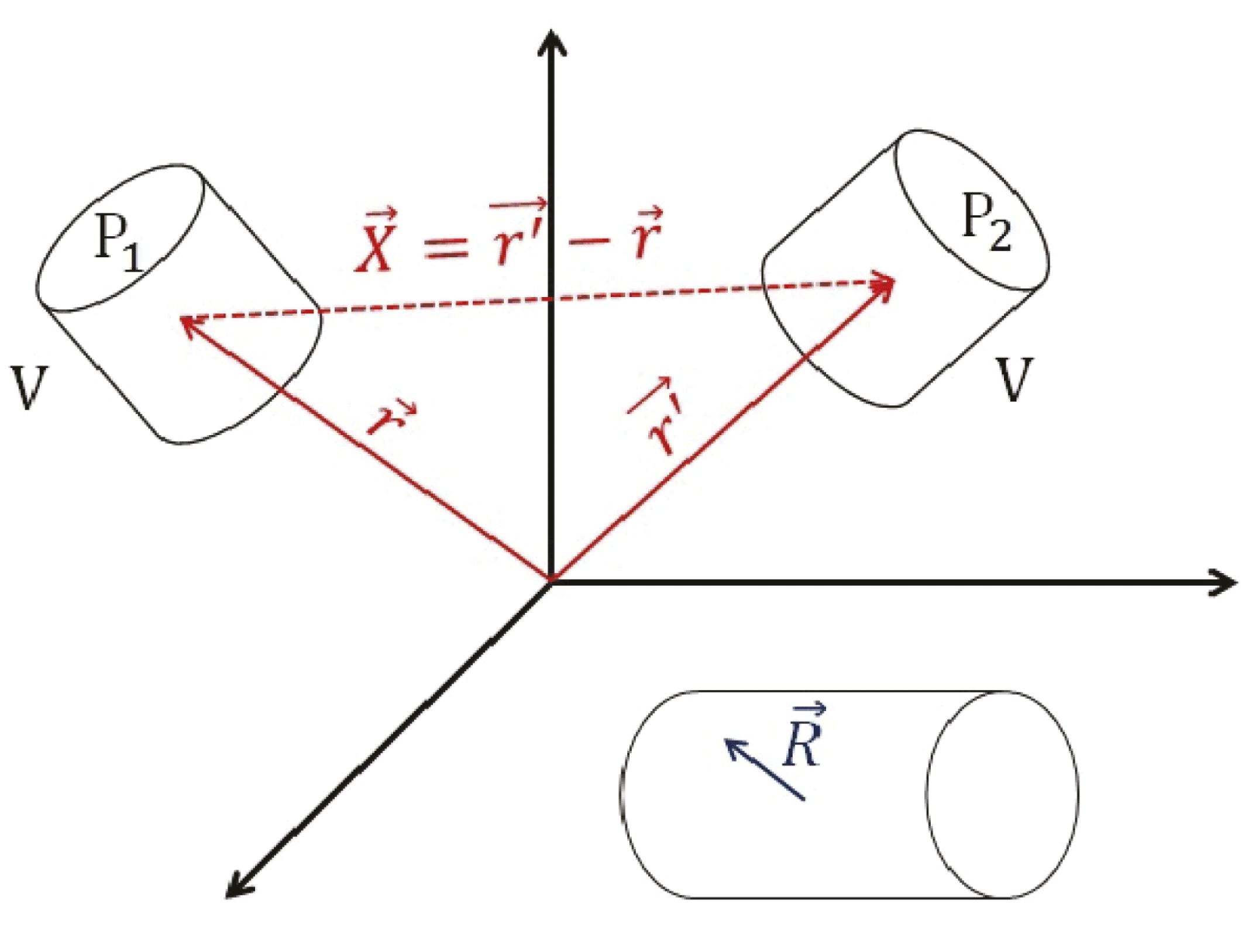
We assume two identical probes $(P_{1},P_{2})$ of volume $V$ embedded in an infinite homogeneous and stationary plasma. Let $\boldsymbol{r},\boldsymbol{r}^{\prime }$ be the constant vectors from the origin of an arbitrary coordinate system to the geometrical centre of the probes, let $\boldsymbol{R}$ be the vector from the probe centres to any point within the probe volumes and let $\boldsymbol{X}$ be the constant vector joining the probe centres $(\boldsymbol{r}^{\prime }=\boldsymbol{r}+\boldsymbol{X})$ , see also figure 1 for an illustration. According to the ansatz of Williams & Chappell (Reference Williams and Chappell1971), probe measurements provide a uniform average of the density over the collecting volume, that within the thin sheath regime (small Debye lengths compared to the probe dimensions) can be assumed to be equal to the probe volume, see also the previous section. We shall refer to this ansatz as the volume average approach. The average of the fluctuating plasma density over the volume of the first probe is given by ${\it\delta}n_{\mathit{m}}^{P_{1}}(\boldsymbol{r},t)=V^{-1}\!\int _{V}{\it\delta}n(\boldsymbol{r}+\boldsymbol{R},t)\,\text{d}V$ . We Fourier transform in space–time $\boldsymbol{r}{-}t$ and use the linear transformation $\boldsymbol{w}=\boldsymbol{r}+\boldsymbol{R}$ . We rearrange the integrals and acquire ${\it\delta}n_{\mathit{m}}^{P_{1}}(\boldsymbol{k},{\it\omega})=[V^{-1}\int _{V}\text{e}^{\text{i}\boldsymbol{k}\boldsymbol{\cdot }\boldsymbol{R}}\,\text{d}V][(2{\rm\pi})^{-4}\int {\it\delta}n(\boldsymbol{w},t)\text{e}^{-\text{i}\boldsymbol{k}\boldsymbol{\cdot }\boldsymbol{w}+\text{i}{\it\omega}t}\,\text{d}^{3}w\,\text{d}t]\,$ . The first bracketed term represents a form factor that depends only on the geometry of the probe, we denote it with $M(\boldsymbol{k})=(V)^{-1}\!\int _{V}\text{e}^{\text{i}\boldsymbol{k}\boldsymbol{\cdot }\boldsymbol{R}}\,\text{d}V$ . The second bracketed term represents the Fourier transformed density fluctuations ${\it\delta}n_{\boldsymbol{k},{\it\omega}}$ . This yields ${\it\delta}n_{\mathit{m}}^{P_{1}}(\boldsymbol{k},{\it\omega})=M(\boldsymbol{k}){\it\delta}n_{\boldsymbol{k},{\it\omega}}$ for the fluctuating density measured by the first probe. Similarly, the volume average of the density fluctuations simultaneously measured by the second probe is given by ${\it\delta}n_{\mathit{m}}^{P_{2}}(\boldsymbol{r}^{\prime },t)=V^{-1}\!\int _{V}{\it\delta}n(\boldsymbol{r}^{\prime }+\boldsymbol{R},t)\,\text{d}V$ . We recall that $\boldsymbol{r}^{\prime }=\boldsymbol{r}+\boldsymbol{X}$ , we Fourier transform in space–time $\boldsymbol{r}{-}t$ and use the linear transformation $\boldsymbol{w}=\boldsymbol{r}+\boldsymbol{X}+\boldsymbol{R}$ . Introducing the form factor, we have ${\it\delta}n_{\mathit{m}}^{P_{2}}(\boldsymbol{k}^{\prime },{\it\omega}^{\prime })=\text{e}^{\text{i}\boldsymbol{k}^{\prime }\boldsymbol{\cdot }\boldsymbol{X}}M(\boldsymbol{k}^{\prime }){\it\delta}n_{\boldsymbol{ k}^{\prime },{\it\omega}^{\prime }}$ for the fluctuating density measured by the second probe.

Figure 1.

Geometry for the calculation of the finite probe size effect. The probe shape can be assumed to be arbitrary, cylindrical probes are chosen for illustrative purposes.

The Fourier transformed space–time correlation function between the two probe volume averages is given by $\langle {\it\delta}n_{\mathit{m}}^{P_{1}}(\boldsymbol{k},{\it\omega}){\it\delta}n_{\mathit{m}}^{P_{2}}(\boldsymbol{k}^{\prime },{\it\omega}^{\prime })\rangle (\boldsymbol{X})$ , it is naturally also a function of the vector $\boldsymbol{X}$ . Combining the above relations, we have $\langle {\it\delta}n_{\mathit{m}}^{P_{1}}(\boldsymbol{k},{\it\omega}){\it\delta}n_{\mathit{m}}^{P_{2}}(\boldsymbol{k}^{\prime },{\it\omega}^{\prime })\rangle (\boldsymbol{X})=\langle \text{e}^{\text{i}\boldsymbol{k}^{\prime }\boldsymbol{\cdot }\boldsymbol{X}}M(\boldsymbol{k}^{\prime })M(\boldsymbol{k}){\it\delta}n_{\boldsymbol{ k},{\it\omega}}{\it\delta}n_{\boldsymbol{k}^{\prime },{\it\omega}^{\prime }}\rangle \,$ . The first three factors are related to the measurement set-up and are independent of the plasma realization, which implies that they can be extracted from the ensemble average. As a consequence of homogeneity–stationarity and by the reality property of the Fourier transform of ${\it\delta}n$ , for the remaining factor we have $\langle {\it\delta}n_{\boldsymbol{k},{\it\omega}}{\it\delta}n_{\boldsymbol{k}^{\prime },{\it\omega}^{\prime }}\rangle =\langle |{\it\delta}n_{\boldsymbol{k},{\it\omega}}|^{2}\rangle {\it\delta}(\boldsymbol{k}+\boldsymbol{k}^{\prime }){\it\delta}({\it\omega}+{\it\omega}^{\prime })$ , where $S_{\boldsymbol{k},{\it\omega}}=\langle |{\it\delta}n_{\boldsymbol{k},{\it\omega}}|^{2}\rangle$ is the spectral density of plasma density fluctuations. This yields $\langle {\it\delta}n_{\mathit{m}}^{P_{1}}(\boldsymbol{k},{\it\omega}){\it\delta}n_{\mathit{m}}^{P_{2}}(\boldsymbol{k}^{\prime },{\it\omega}^{\prime })\rangle (\boldsymbol{X})=\text{e}^{-\text{i}\boldsymbol{k}\boldsymbol{\cdot }\boldsymbol{X}}|M(\boldsymbol{k})|^{2}S_{\boldsymbol{k},{\it\omega}}{\it\delta}(\boldsymbol{k}+\boldsymbol{k}^{\prime }){\it\delta}({\it\omega}+{\it\omega}^{\prime })\,$ . Clearly, for single probe measurements, we have $\boldsymbol{X}=0$ . Using the typical definitions $\langle {\it\delta}n_{\mathit{m}}^{P_{1}}(\boldsymbol{k},{\it\omega}){\it\delta}n_{\mathit{m}}^{P_{2}}(\boldsymbol{k}^{\prime },{\it\omega}^{\prime })\rangle (0)=\langle |{\it\delta}n_{\mathit{m}}^{P}(\boldsymbol{k},{\it\omega})|^{2}\rangle (0){\it\delta}(\boldsymbol{k}+\boldsymbol{k}^{\prime }){\it\delta}({\it\omega}+{\it\omega}^{\prime })$ and $S_{\boldsymbol{k},{\it\omega}}^{\mathit{m}}=\langle |{\it\delta}n_{\mathit{m}}^{P}(\boldsymbol{k},{\it\omega})|^{2}\rangle (0)$ , we obtain $S_{\boldsymbol{k},{\it\omega}}^{\mathit{m}}=|M(\boldsymbol{k})|^{2}S_{\boldsymbol{k},{\it\omega}}$ (Williams & Chappell Reference Williams and Chappell1971). Finally, after normalizing with respect to the average density value $\langle n\rangle$ , we end up with $\widetilde{S}_{\boldsymbol{k},{\it\omega}}^{\mathit{m}}=|M(\boldsymbol{k})|^{2}\widetilde{S}_{\boldsymbol{k},{\it\omega}}$ . The result is general, but since in this work we are interested in ion density fluctuations, we shall rewrite it explicitly as

(4.1) $$\begin{eqnarray}\widetilde{S}_{\boldsymbol{k},{\it\omega}}^{\mathit{m}}=|M(\boldsymbol{k})|^{2}\widetilde{S}_{\boldsymbol{ k},{\it\omega}}^{\mathit{i}}.\end{eqnarray}$$

The form factor $|M(\boldsymbol{k})|^{2}$ quantifies the effect of the finite probe size, it expresses the fact that probes cannot equally resolve all wavenumbers. It is straightforward to show that for an infinitesimal probe ( $\boldsymbol{R}\rightarrow 0$ ) the form factor tends to unity. Notice that, had we neglected the finite probe size, the Fourier transform of the time correlation function of the ion density would be given by $\widetilde{S}_{{\it\omega}}^{\mathit{i}}=\int \!\widetilde{S}_{\boldsymbol{k},{\it\omega}}^{\mathit{i}}\,\text{d}^{3}k$ . Consequently, the theoretical expression for the Fourier transform of the measured time correlation function is given by $\widetilde{S}_{{\it\omega}}^{\mathit{m}}=\int \!\widetilde{S}_{\boldsymbol{k},{\it\omega}}^{\mathit{m}}\,\text{d}^{3}k$ or equivalently by

(4.2) $$\begin{eqnarray}\widetilde{S}_{{\it\omega}}^{\mathit{m}}=\int |M(\boldsymbol{k})|^{2}\widetilde{S}_{\boldsymbol{ k},{\it\omega}}^{\mathit{i}}\,\text{d}^{3}k.\end{eqnarray}$$

We shall now discuss the appropriate physical integration limits, that mathematically should be from zero to infinity. We begin with the consideration of the long-wavelength limit. It follows directly that the form factor tends to unity for $k\rightarrow 0$ . The large argument expansion of the plasma dispersion function (Fried & Conte Reference Fried and Conte1961) leads to ${\it\chi}_{\boldsymbol{k},{\it\omega}}^{{\it\alpha}}=-{\it\omega}_{\mathit{p}{\it\alpha}}^{2}/{\it\omega}^{2}$ , which are the cold plasma susceptibilities, since for $k\rightarrow 0$ thermal effects can be neglected. Therefore, the spectral density of ion density fluctuations, (2.9), behaves as $\widetilde{S}_{\boldsymbol{k},{\it\omega}}^{\mathit{i}}\propto (1/k)\exp (-{\it\omega}^{2}/2k^{2}v_{T{\it\alpha}}^{2})$ and the integral converges at $k\rightarrow 0$ . We continue with the consideration of the short-wavelength limit. By employing the small argument expansion of the plasma dispersion function (Fried & Conte Reference Fried and Conte1961), we have ${\it\chi}_{\boldsymbol{k},{\it\omega}}^{{\it\alpha}}=1/k^{2}{\it\lambda}_{\mathit{D}{\it\alpha}}^{2}\rightarrow 0$ , which are the static plasma susceptibilities, since for $k\rightarrow \infty$ all frequency effects can be neglected. Therefore, the spectral density of ion density fluctuations, (2.9), behaves as $\widetilde{S}_{\boldsymbol{k},{\it\omega}}^{\mathit{i}}\propto 1/k$ . This implies that, in absence of the form factor, the integral $\widetilde{S}_{{\it\omega}}^{\mathit{i}}=\int \!\widetilde{S}_{\boldsymbol{k},{\it\omega}}^{\mathit{i}}\,\text{d}^{3}k$ diverges at infinity. By utilizing the plane wave expansion of $\text{e}^{\text{i}\boldsymbol{k}\boldsymbol{\cdot }\boldsymbol{R}}$ in spherical harmonics, it can be shown in a general manner that with the addition of the form factor the integral $\int \!|M(\boldsymbol{k})|^{2}\widetilde{S}_{\boldsymbol{k},{\it\omega}}^{\mathit{i}}\,\text{d}^{3}k$ converges at $k\rightarrow \infty$ . But the short-wavelength limit should also be viewed in light of the assumptions of fluctuation theory. In the case of classical plasmas, for very short distances, less than the so-called Coulomb radius $R_{\mathit{c}}$ that corresponds to the distance at which the kinetic energy of a particle is equal to its potential energy, linear theory breaks down (Klimontovich Reference Klimontovich1982). Consequently, strictly speaking, $k_{\mathit{m}}=R_{\mathit{c}}^{-1}$ is the physical upper integration limit similar to the case of the Landau collision integral (Montgomery & Tidman Reference Montgomery and Tidman1964; Schram Reference Schram1991). However, the probe dimensions are many orders of magnitude larger than the Coulomb radius and for typical probe geometries, the form factor is a rapidly decaying oscillating function of the wavenumber normalized by the probe dimensions. Hence, for $k\sim R_{\mathit{c}}^{-1}$ the integrand is already effectively zero and the mathematical integration limits can be employed.

4.2 Form factor for cylindrical probes

We shall compute the explicit form of the form factor for a cylindrical probe of radius $R_{\mathit{p}}$ and length $L_{\mathit{p}}$ , $V={\rm\pi}R_{\mathit{p}}^{2}L_{\mathit{p}}$ . We employ cylindrical coordinates $\boldsymbol{R}=({\it\rho},{\it\phi},z)$ and without loss of generality assume that the wavenumber lies in the $y$ – $z$ plane, which leads to $\boldsymbol{k}\boldsymbol{\cdot }\boldsymbol{R}=k_{\Vert }z+k_{\bot }{\it\rho}\sin {\it\phi}$ and $\,\text{d}V=\,\text{d}^{3}R={\it\rho}\,\text{d}{\it\phi}\,\text{d}{\it\rho}\,\text{d}z$ . The polar integration is carried out with the aid of Parseval’s integral $2{\rm\pi}\text{J}_{0}(a)=\int _{0}^{2{\rm\pi}}\exp (\text{i}a\sin {\it\phi})\text{d}{\it\phi}$ with $\text{J}_{n}(a)$ denoting the Bessel function of the first kind and $n$ th order. The radial integration is carried out with the aid of the Bessel function properties $\text{d}/\text{d}x\,[x\text{J}_{1}(x)]=x\text{J}_{0}(x)$ and $\text{J}_{1}(0)=0$ , whereas the axial integration is trivial. Overall, we have

(4.3) $$\begin{eqnarray}M_{\mathit{c}}(k_{\Vert },k_{\bot })=\frac{\sin \left(k_{\Vert }L_{\mathit{p}}/2\right)}{\left(k_{\Vert }L_{\mathit{p}}/2\right)}\,\frac{\text{J}_{1}\left(k_{\bot }R_{\mathit{p}}\right)}{\left(k_{\bot }R_{\mathit{p}}/2\right)}.\end{eqnarray}$$

Clearly, the form factor is naturally factorized into two partial form factors $M_{\mathit{c}}(k_{\Vert },k_{\bot })=M_{\mathit{c}\Vert }(k_{\Vert })M_{\mathit{c}\bot }(k_{\bot })$ , where the axial part is given by $M_{\mathit{c}\Vert }(k_{\Vert })=\sin (k_{\Vert }L_{\mathit{p}}/2)/(k_{\Vert }L_{\mathit{p}}/2)$ and the radial part is given by $M_{\mathit{c}\bot }(k_{\bot })=\text{J}_{1}(k_{\bot }R_{\mathit{p}})/(k_{\bot }R_{\mathit{p}}/2)$ . The partial form factors are rapidly decaying oscillating functions of the relevant wavenumber projection and have the property $\max \{M_{\mathit{c}\Vert }(k_{\Vert })\}=M_{\mathit{c}\Vert }(0)=1$ and $\max \{M_{\mathit{c}\bot }(k_{\bot })\}=M_{\mathit{c}\bot }(0)=1$ . With the input of (4.3), the Fourier transform of the measured time correlation function, (4.2), becomes

(4.4) $$\begin{eqnarray}\widetilde{S}_{{\it\omega}}^{\mathit{m}}=2{\rm\pi}\int _{0}^{\infty }\int _{0}^{\infty }M_{\mathit{c}\Vert }^{2}(k_{\Vert })M_{\mathit{c}\bot }^{2}(k_{\bot })\widetilde{S}^{\mathit{i}}\left(\sqrt{k_{\Vert }^{2}+k_{\bot }^{2}},{\it\omega}\right)k_{\bot }\,\text{d}k_{\bot }\,\text{d}k_{\Vert },\end{eqnarray}$$

where we employed $\widetilde{S}_{\boldsymbol{k},{\it\omega}}^{\mathit{i}}=\widetilde{S}_{|\boldsymbol{k}|,{\it\omega}}^{\mathit{i}}=\widetilde{S}^{\mathit{i}}(k,{\it\omega})$ due to the fact that the homogeneous plasma is isotropic in absence of external electromagnetic fields and carried out the integration over the polar angle. In the literature, the finite probe size effect is typically not considered in the rigorous manner presented above and artificial wavenumber cutoffs are introduced (Gunell & Skiff Reference Gunell and Skiff2002; Li & Hazeltine Reference Li and Hazeltine2006; Ratynskaia et al. Reference Ratynskaia, de Angeli, Lazzaro, Marmolino, de Angelis, Castaldo, Cremona, Laguardia, Gervasini and Grosso2010; Pécseli Reference Pécseli2015) that might not always be appropriate. In thermal fluctuation measurements (Gunell & Skiff Reference Gunell and Skiff2002; Ratynskaia et al. Reference Ratynskaia, de Angeli, de Angelis, Marmolino, Capobianco, Lontano, Lazzaro, Morfill and Gervasini2007), the logical assumption made is that wavelengths much smaller than the probe dimensions will be averaged out, which leads to the somewhat arbitrary upper integration limits $k_{\Vert ,\mathit{m}}=2{\rm\pi}/(L_{\mathit{p}}/2)$ and $k_{\bot ,\mathit{m}}=2{\rm\pi}/R_{\mathit{p}}$ . By utilizing the properties of the Heaviside step function, these cutoff wavenumbers can be shown to correspond to the partial form factors $M_{\mathit{c}\Vert }(k_{\Vert })=\text{H}(k_{\Vert ,\mathit{m}}-k_{\Vert })$ and $M_{\mathit{c}\bot }(k_{\bot })=\text{H}(k_{\bot ,\mathit{m}}-k_{\bot })$ . 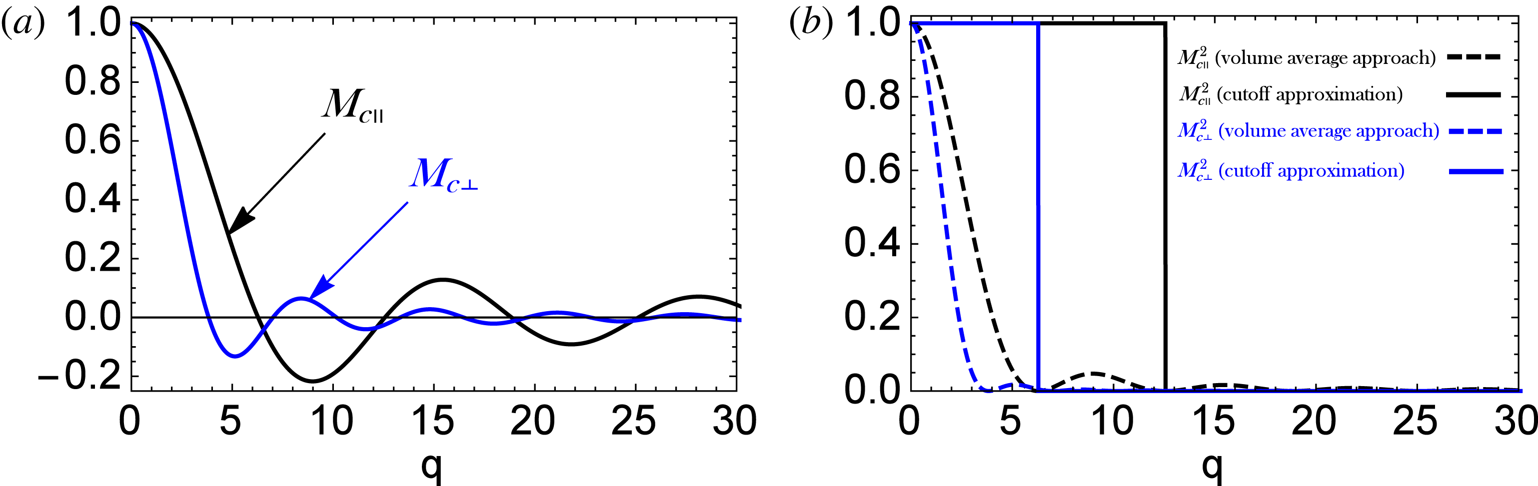As illustrated in figure 2, the cutoff wavenumber approximation can lead to a significant overestimation for the case of a cylindrical probe.

Figure 2.

The partial form factors for a cylindrical probe as functions of the dimensionless wavenumbers $q_{\Vert }=k_{\Vert }L_{\mathit{p}}$ and $q_{\bot }=k_{\bot }R_{\mathit{p}}$ . For the treatment within the volume average approach, they follow the expressions $M_{\mathit{c}\Vert }(q_{\Vert })=\sin (q_{\Vert }/2)/(q_{\Vert }/2)$ and $M_{\mathit{c}\bot }(q_{\bot })=\text{J}_{1}(q_{\bot })/(q_{\bot }/2)$ . For the cutoff approximation, they follow the expressions $M_{\mathit{c}\Vert }(q_{\Vert })=\text{H}(4{\rm\pi}-q_{\Vert })$ and $M_{\mathit{c}\bot }(q_{\bot })=\text{H}(2{\rm\pi}-q_{\bot })$ . (a) Plots of $M_{\mathit{c}\Vert },M_{\mathit{c}\bot }$ stemming from the volume average approach. The first zero crossings occur at $q_{\bot ,z}\simeq 3.83$ and $q_{\Vert ,z}=2{\rm\pi}$ . (b) Plots of $M_{\mathit{c}\Vert }^{2},M_{\mathit{c}\bot }^{2}$ stemming from both treatments. Notice that there is no cutoff wavenumber selection that can realistically approximate any of the bell-shaped functions.

4.3 Form factor for spherical probes

We shall compute the explicit form of the form factor for a spherical probe of radius $R_{\mathit{p}}$ , $V=(4/3){\rm\pi}R_{\mathit{p}}^{3}$ . We employ spherical coordinates $\boldsymbol{R}=({\it\rho},{\it\theta},{\it\phi})$ and without loss of generality assume that the wavenumber is parallel to the $z$ axis, which leads to $\boldsymbol{k}\boldsymbol{\cdot }\boldsymbol{R}=k{\it\rho}\cos {\it\theta}$ and $\,\text{d}V=\,\text{d}^{3}R={\it\rho}^{2}\sin {\it\theta}\,\text{d}{\it\phi}\,\text{d}{\it\theta}\,\text{d}{\it\rho}$ . We obtain

(4.5) $$\begin{eqnarray}M_{\mathit{s}}(k)=\frac{3}{k^{3}R_{\mathit{p}}^{3}}[\sin (kR_{\mathit{p}})-(kR_{\mathit{p}})\cos (kR_{\mathit{p}})].\end{eqnarray}$$

The form factor is a rapidly decaying oscillating function of $k$ that has the property $\max \{M_{\mathit{s}}(k)\}=M_{\mathit{s}}(0)=1$ . With the input of (4.5), the Fourier transform of the measured time correlation function, (4.2), becomes

(4.6) $$\begin{eqnarray}\widetilde{S}_{{\it\omega}}^{\mathit{m}}=4{\rm\pi}\int _{0}^{\infty }M_{\mathit{s}}^{2}(k)\widetilde{S}^{\mathit{i}}(k,{\it\omega})k^{2}\,\text{d}k,\end{eqnarray}$$

where we employed $\widetilde{S}_{\boldsymbol{k},{\it\omega}}^{\mathit{i}}=\widetilde{S}^{\mathit{i}}(k,{\it\omega})$ due to isotropy and carried out the integrations over the azimuthal and inclination angles. Treatment of the finite probe size effect in a heuristic manner, as described above, would lead to the upper integration limit $k_{\mathit{m}}=2{\rm\pi}/R_{\mathit{p}}$ . Such a cutoff wavenumber corresponds to the form factor $M_{\mathit{s}}(k)=\text{H}(k_{\mathit{m}}-k)$ . 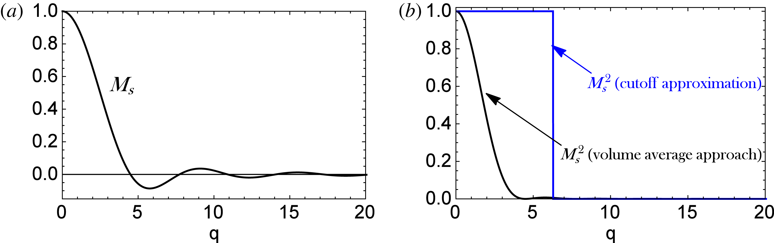As illustrated in figure 3, the cutoff wavenumber approximation can lead to a significant overestimation also for the case of a spherical probe.

Figure 3.

The form factor for a spherical probe as a function of the dimensionless wavenumber $q=kR_{\mathit{p}}$ . For the treatment within the volume average approach, it follows the expression $M_{\mathit{s}}(q)=(3/q^{3})(\sin q-q\cos q)$ . For the cutoff approximation, it follows the expression $M_{\mathit{s}}(q)=\text{H}(2{\rm\pi}-q)$ . (a) Plot of $M_{\mathit{s}}$ stemming from the volume average approach. The first zero crossing occurs at $q_{z}\simeq 4.49$ . (b) Plots of $M_{\mathit{s}}^{2}$ stemming from both treatments. Notice that there is no cutoff wavenumber selection that can realistically approximate the bell-shaped function.

Figure 4.

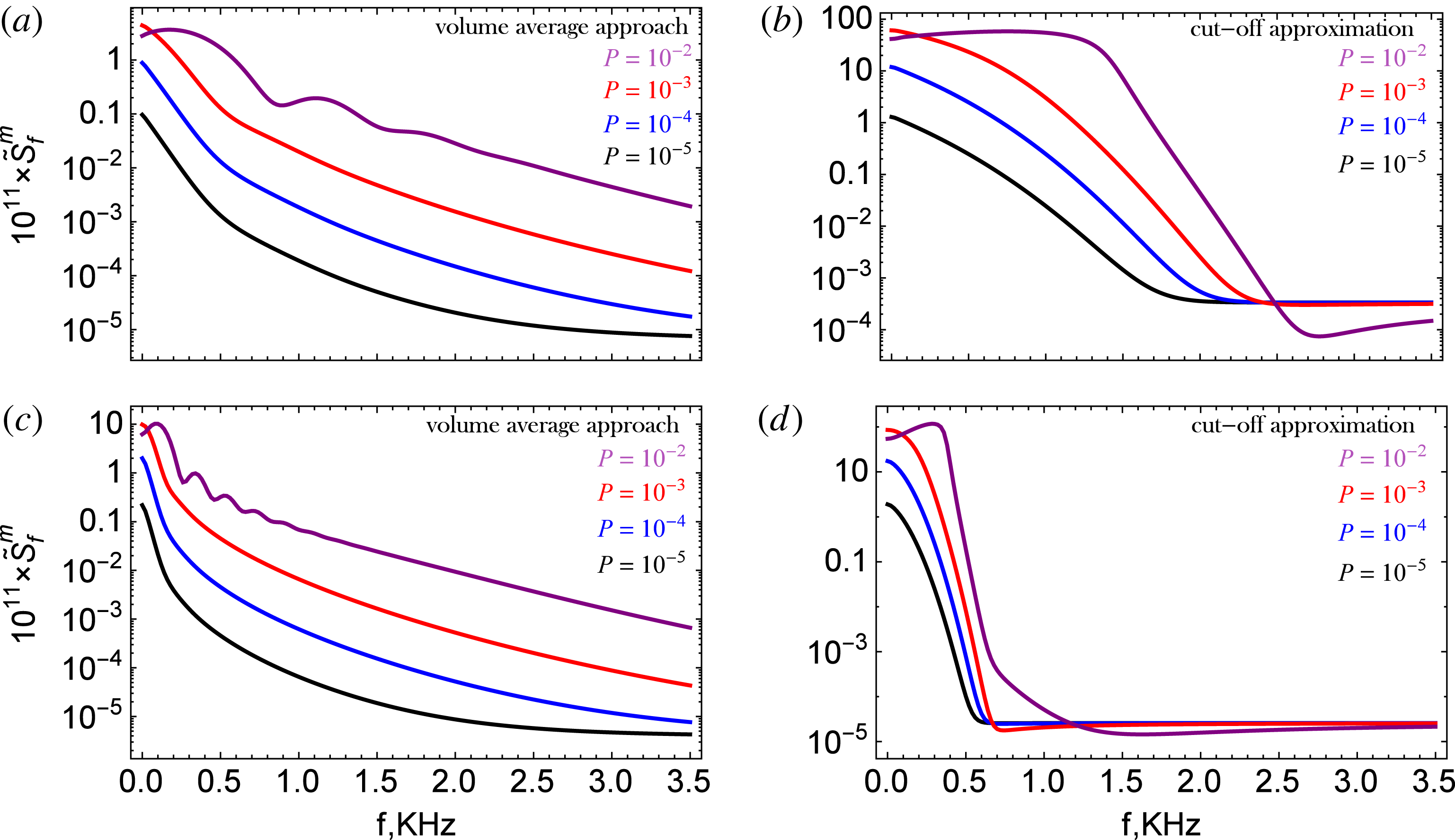
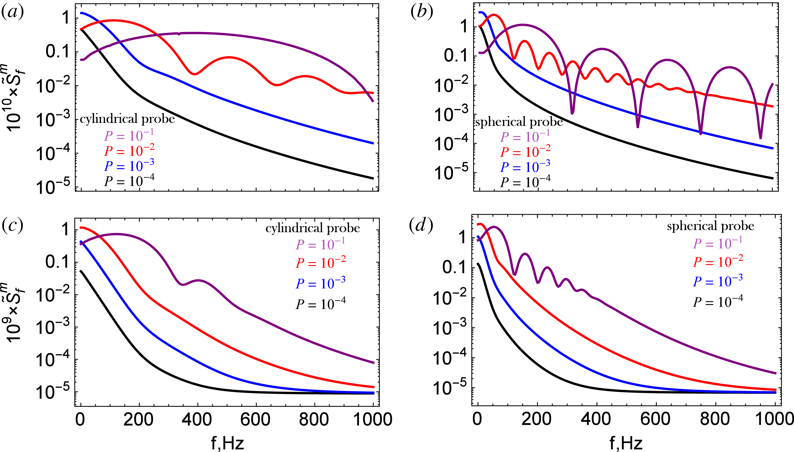
The wavenumber-integrated normalized spectral density of ion density fluctuations for constant dust radius $R_{\mathit{d}}=100\,$ nm and varying dust density from $2\times 10^{3}$ to $2\times 10^{6}~\text{cm}^{-3}$ . The Argon plasma parameters relevant for the magnetic cusp device are $n_{\mathit{i}}=10^{11}~\text{cm}^{-3}$ , $T_{\mathit{e}}=3~\text{eV}$ ,  $T_{\mathit{i}}(=T_{\mathit{d}})=0.03~\text{eV}$ and the dust mass density is ${\it\rho}_{\mathit{d}}=1.8~\text{g}~\text{cm}^{-3}$ . For decreasing dust densities, the plasma frequencies $f_{\mathit{pd}}$ are (2200, 700, 220, 70) Hz, the characteristic charge number $Z_{\mathit{d}}\sim 500$ and the parameter $PZ_{\mathit{d}}$ is $(5,0.5,0.05,0.005)$ . The finite probe size effect is considered following the volume average approach and the cutoff approximation. Results for (a,b) cylindrical probe with $L_{\mathit{p}}=0.2~\text{cm}$ , $R_{\mathit{p}}=0.005~\text{cm}$ (c,d) spherical probe with $R_{\mathit{p}}=0.02$  cm.

Figure 5.

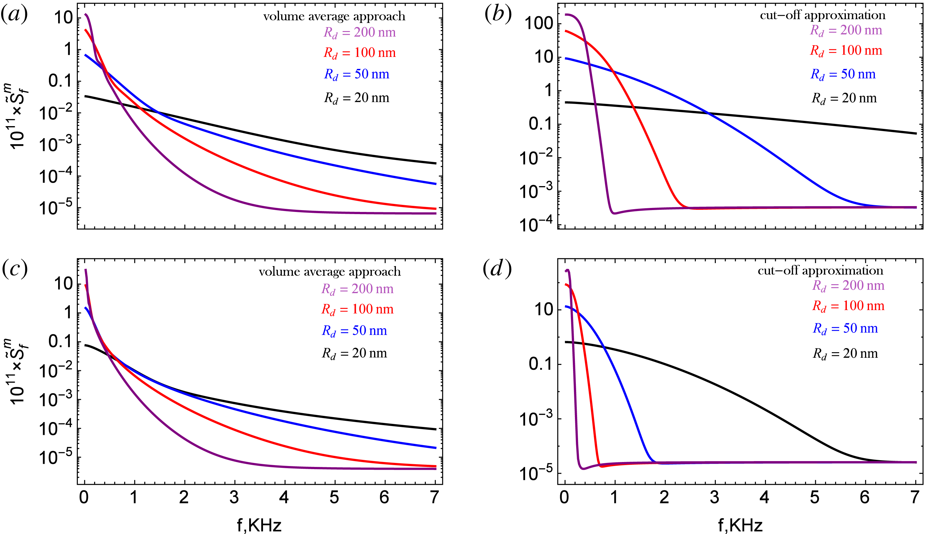
The wavenumber-integrated normalized spectral density of ion density fluctuations for constant dust density $n_{\mathit{d}}=2\times 10^{5}~\text{cm}^{-3}$ and varying dust radius from 20 to 200 nm. The Argon plasma parameters relevant for the magnetic cusp device are $n_{\mathit{i}}=10^{11}~\text{cm}^{-3}$ ,  $T_{\mathit{e}}=3~\text{eV}$ , $T_{\mathit{i}}(=T_{\mathit{d}})=0.03~\text{eV}$ and the dust mass density is ${\it\rho}_{\mathit{d}}=1.8~\text{g}~\text{cm}^{-3}$ . For increasing dust sizes, the plasma frequencies $f_{\mathit{pd}}$ are $(1560,\,990,\,700,\,495)$  Hz,  $Z_{\mathit{d}}$ is $(100,250,500,1000)$ and $PZ_{\mathit{d}}$ is $(0.02,0.13,0.5,2)$ . The finite probe size effect is considered following the volume average approach and the cutoff approximation. Results for (a,b) cylindrical probe with $L_{\mathit{p}}=0.2~\text{cm}$ , $R_{\mathit{p}}=0.005~\text{cm}$ (c,d) spherical probe with $R_{\mathit{p}}=0.02~\text{cm}$ .

Figure 6.

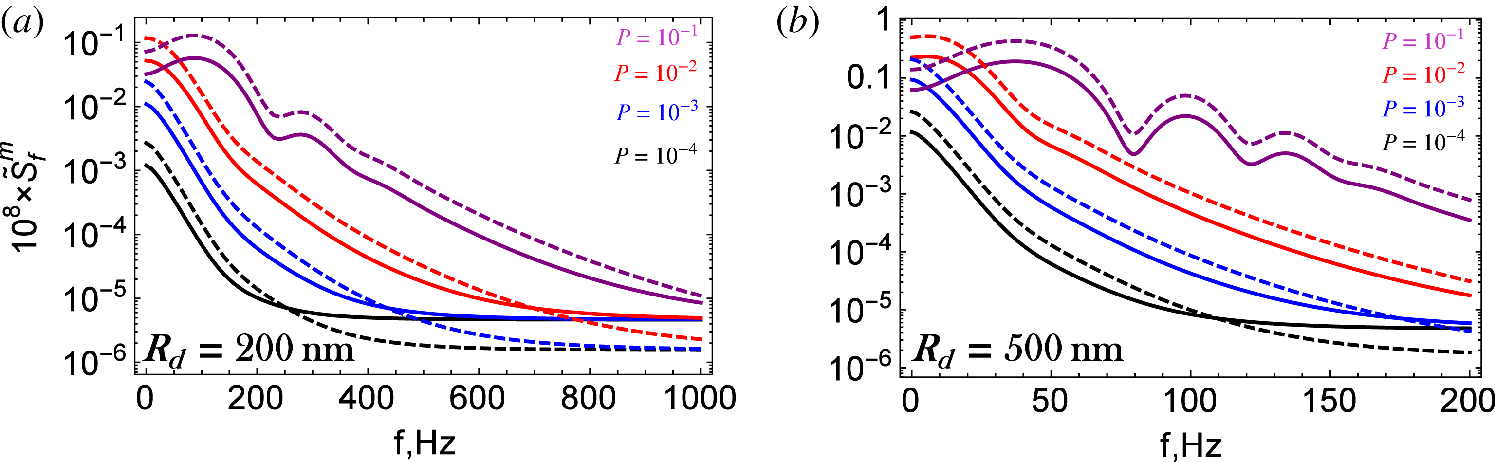
The wavenumber-integrated normalized spectral density of ion density fluctuations for constant dust radius $R_{\mathit{d}}=200\,$ nm, dust mass density ${\it\rho}_{\mathit{d}}=1.8~\text{g}~\text{cm}^{-3}$ and varying dust number density. The finite probe size effect is considered following the volume average approach. Results for cylindrical probe with $L_{\mathit{p}}=0.2~\text{cm}$ , $R_{\mathit{p}}=0.005~\text{cm}$ (a,c) and spherical probe with $R_{\mathit{p}}=0.02~\text{cm}$ (b,d). (a,b) The Argon plasma parameters relevant for the magnetic cusp device are $n_{\mathit{i}}=10^{11}~\text{cm}^{-3}$ , $T_{\mathit{e}}=3~\text{eV}$ and $T_{\mathit{i}}~(=T_{\mathit{d}})=0.03~\text{eV}$ . The dust densities vary from $10^{7}$ to $10^{4}~\text{cm}^{-3}$ , the corresponding plasma frequencies $f_{\mathit{pd}}$ are $(3440,\,1100,\,350,\,110)$  Hz,  $Z_{\mathit{d}}\sim 1000$ and $PZ_{\mathit{d}}$ is $(100,10,1,0.1)$ . (c,d) The Argon plasma parameters relevant for the brush cathode device are $n_{\mathit{i}}=10^{10}~\text{cm}^{-3}$ , $T_{\mathit{e}}=0.3~\text{eV}$ and $T_{\mathit{i}}~(=T_{\mathit{d}})=0.03~\text{eV}$ . The dust densities vary from $7.5\times 10^{6}$ to $7.5\times 10^{3}~\text{cm}^{-3}$ , the corresponding plasma frequencies $f_{\mathit{pd}}$ are $(400,\,128,\,40,\,13)$  Hz,  $Z_{\mathit{d}}\sim 135$ and $PZ_{\mathit{d}}$ is $(13.5,1.35,0.135,0.0135)$ .