


INTRODUCTION
Lianas (woody climbers) are plants that rely on other structures for physical support to reach the canopy, and keep connected to the ground (Gerwing et al. Reference GERWING, SCHNITZER, BURNHAM, BONGERS, CHAVE, DEWALT, EWANGO, FOSTER, KENFACK, MARTÍNEZ-RAMOS, PARREN, PARTHASARATHY, PÉREZ-SALICRUP, PUTZ and THOMAS2006). Field research suggests that lianas have important roles in forest ecosystems, such as in species diversity (Gentry Reference GENTRY, Putz and Mooney1991), primary production (Phillips et al. Reference PHILLIPS, MARTÍNEZ, MENDOZA, BAKER and VARGAS2005) and forest dynamics (Schnitzer & Bongers Reference SCHNITZER and BONGERS2002, Schnitzer et al. Reference SCHNITZER, DALLING and CARSON2000). Abundance of lianas varies among forest types (Hegarty & Caballé Reference HEGARTY, CABALLÉ, Putz and Mooney1991) and within a forest type (Putz Reference PUTZ1984). Many studies have focused on variation of liana community structure among different forest types (DeWalt et al. Reference DEWALT, SCHNITZER and DENSLOW2000, Reference DEWALT, ICKES, NILUS, HARMS and BURSLEM2006; Ibarra-Manríquez & Martínez-Ramos Reference IBARRA-MANRÍQUEZ and MARTÍNEZ-RAMOS2002). Few studies have reported variation of abundance of lianas within a forest type (Kusumoto & Enoki Reference KUSUMOTO and ENOKI2008, Putz Reference PUTZ1984, Putz & Chai Reference PUTZ and CHAI1987).
Distribution and abundance of lianas are affected by several environmental factors (Schnitzer & Bongers Reference SCHNITZER and BONGERS2002) and disturbance regimes (Babweteera et al. Reference BABWETEERA, PLUMPTRE and OBUA2000, Kouamé et al. Reference KOUAMÉ, BONGERS, POORTER and TRAORÉ2004). For example, field research has suggested that abundance of lianas is positively related to soil fertility (Laurance et al. Reference LAURANCE, PÉREZ-SALICRUP, DELAMÔNICA, FEARNSIDE, D'ANGELO, JEROZOLINSKI, POHL and LOVEJOY2001), soil water (Ibarra-Manríquez & Martínez-Ramos Reference IBARRA-MANRÍQUEZ and MARTÍNEZ-RAMOS2002), or canopy openness (Babweteera et al. Reference BABWETEERA, PLUMPTRE and OBUA2000). Disturbances such as tree fall can increase abundance of lianas, partly due to increase in light availability (DeWalt et al. Reference DEWALT, SCHNITZER and DENSLOW2000, Hegarty & Caballé Reference HEGARTY, CABALLÉ, Putz and Mooney1991, Putz Reference PUTZ1984).
Topography is one of the most important factors affecting water and nutrient conditions in soils (Brubaker et al. Reference BRUBAKER, JONES, LEWIS and FRANK1993, Gessler et al. Reference GESSLER, CHADWICK, CHARMRAN, ALTHOUSE and HOLMES2000, Hazlett & Foster Reference HAZLETT and FOSTER2002, Roy & Singh Reference ROY and SINGH1994), solar radiation (Hayes et al. Reference HAYES, MOODY, WHITE and COSTANZA2007), and disturbance regimes (Hunter & Parker Reference HUNTER and PARKER1993, Nagamatsu & Miura Reference NAGAMATSU and MIURA1997). Spatial variation in these factors caused by topography can affect the composition and structure of stands (Enoki Reference ENOKI2003, Kubota et al. Reference KUBOTA, MURATA and KIKUZAWA2004, Nagamatsu & Miura Reference NAGAMATSU and MIURA1997, Tateno & Takeda Reference TATENO and TAKEDA2003, Webb et al. Reference WEBB, STANFIELD and JENSEN1999). Putz & Chai (Reference PUTZ and CHAI1987) reported that composition and structure of liana communities varied with topography in a tropical forest in Malaysia.
The subtropical evergreen broad-leaved forest in the northern part of the main island of Okinawa, south-western Japan, has highly variable topography. Species composition and structure of the stands vary with topography (Enoki Reference ENOKI2003, Kubota et al. Reference KUBOTA, MURATA and KIKUZAWA2004). The distributions of tree species in the forest are related to topographic factors, such as slope angle and/or relief at a small spatial scale (5 m × 5 m) (Enoki Reference ENOKI2003). Although there have been no studies on liana communities in the region to date, topography may also significantly affect distribution and abundance of lianas.
In the present study, we studied community structure and distribution of lianas in a watershed in an evergreen broad-leaved forest on Okinawa. We examined distribution and abundance in relation to topography for total species and for each species. Three topographic factors were considered: slope angle, slope aspect and relief. We analysed cell data produced by geographical information systems (GIS) to clarify topographic factors that result in spatial variation of liana distribution within the forest. Because the study at the watershed level was expected to contain many cells without lianas, we analysed distribution and abundance separately.
To determine whether slope angle, slope aspect and relief affect distribution of lianas, we analysed liana distribution using presence/absence data from each cell. To determine whether topographic factors affect liana abundance, we analysed variation in liana abundance using stem density data, excluding cells without lianas.
SITE DESCRIPTION
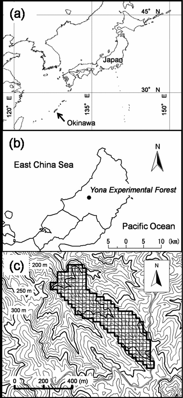
The study was conducted in a mountainous region of the Yona Experimental Forest, University of the Ryukyus, in the northern part of the main island of Okinawa, south-western Japan (26°44′N, 128°14′E; Figure 1a, b). The climate of the area is maritime subtropical. The mean annual temperature is 22.3 °C and the mean annual precipitation is 2550 mm (Yona Experimental Forest). The mean temperature of the coldest month is 17.5 °C (January) and the warmest month, 29.4 °C (August). Monthly precipitation ranges from 150 mm to 300 mm. The island receives monsoons from the south-east during May to August and from the north-west during October to March. Typhoons frequently hit the area between July and October. The topography of the area is hilly and dissected. The bedrock is composed of sandstone and clay-slate. The soil is a yellow forest soil lacking humus layer development.
Geographic, regional and local map of study site. Map of Japan and geographical location of Okinawa (indicated with an arrow) with latitude and longitude lines (a). Map of the northern part of the main island of Okinawa and the location of the Yona Experimental Forest, University of the Ryukyus (b). Topographic map around the study watershed (c). Area framed with a solid line indicates the study watershed, divided into 25-m cells with thin lines. Contour lines are shown at 10-m intervals. Maps of Okinawa were drawn using data sourced from Global Map-Japan (abridged edition) version 1.1. (International Steering Committee for Global Mapping).
The subtropical evergreen broad-leaved forest in the region has high species diversity among canopy species (Itô Reference ITÔ1997). The forest canopy is dominated by evergreen broad-leaved tree species, such as Castanopsis sieboldii, Schima wallichii and Distylium racemosum (Enoki Reference ENOKI2003, Kubota et al. Reference KUBOTA, KATSUDA and KIKUZAWA2005). Intensive logging has been conducted in a large area of the northern part of Okinawa over the past 50 y. Most parts of the forest in the area are secondary forest that has regenerated after past disturbances (Kubota et al. Reference KUBOTA, KATSUDA and KIKUZAWA2005). Species nomenclature follows Satake et al. (Reference SATAKE, HARA, WATARI and TOMINARI1989a, Reference SATAKE, HARA, WATARI and TOMINARIb) and Hatusima & Amano (Reference HATUSIMA and AMANO1994).
A watershed in the Yona Experimental Forest was selected as the study site (Figure 1c). The watershed is located on the upper-stream of the Yona River, and is approximately 16 ha in area. The altitude of the study area ranged from 179.0 m to 314.5 m asl. According to records of the Experimental Forest, the forest has no history of logging or other artificial disturbance in the past 50 y. Logging was carried out before that period in the forest, but details of the logging events were never recorded.
METHODS
GIS data processing
The study area was divided into 257 cells, each 25 m × 25 m (16.0625 ha), on the rectangular plane coordinate system (Japan Coordinate System, Japan Plate Carree JGD 2000, zone XV). In the present study, surface features ranging from several metres to several hundred metres, for example ridge and valley, were treated as topographic features. Three topographical parameters – slope angle, slope aspect index (SAI) and relief index (RI) – were calculated for each cell using 10 m × 10-m digital elevation models (DEM). The DEM was produced on the basis of a contour map with 10-m intervals created by the Geographical Institute of Japan (GISMAP Terrain ver. 2.0, Hokkaido-Chizu Co., Ltd, Hokkaido, Japan). For each DEM point, the topographic parameters were calculated. Each point's slope angle was calculated using an inclination of a plane vector constructed from the surrounding eight points. Slope azimuth was the compass direction (0–360°) of a normal line projected on a horizontal plane for a plane vector. In addition, the slope azimuths were transformed into SAI using the following equation.

where a are slope azimuths of the point. SAI implies that north was zero and south was 100, so that SAI could be treated as a quantitative variable. Before the calculation of RI, concavity and convexity were calculated. Concavity and convexity are indices of the relief of the land surface, based on the concept described by Yokoyama et al. (Reference YOKOYAMA, SHIRASAWA and PIKE2002). For each of eight azimuths, elevation angle between a target point and the highest point within 100 m was defined as maximum elevation angle, and that between the target point and the lowest point within 100 m was defined as minimum elevation angle. Angles below the horizontal were treated as negative values. Concavity was defined as sum of the eight maximum elevation angles. Convexity was defined as sum of the eight minimum elevation angles. We calculated RI so that concavity and convexity could be combined as one variable. The RIs were calculated using the following equation:

In the RI, 0 indicates a flat plane, and positive and negative values indicate convex and concave topography, respectively. In a mountainous region, RI values are highest at a ridge top, and lowest at a valley bottom. After the calculations, the parameters were added to 25 m cell data using overlay analysis.
Field measurements
All liana stems ≥ 2 cm in diameter at 1.3 m point from their root were marked and inventoried. Their diameter was measured according to Gerwing et al. (Reference GERWING, SCHNITZER, BURNHAM, BONGERS, CHAVE, DEWALT, EWANGO, FOSTER, KENFACK, MARTÍNEZ-RAMOS, PARREN, PARTHASARATHY, PÉREZ-SALICRUP, PUTZ and THOMAS2006), and their root position was recorded. Diameter was measured at 1.3 m point from their main root. In the case where adventitious roots emerged more than 1.3 m from the main root, we measured 0.5 m above the highest adventitious root. Where branching of lianas occurred close to the ground, each branch was measured separately at 1.3 m, and recorded as a multiple stem. Further details of the measurement of lianas can found in Gerwing et al. (Reference GERWING, SCHNITZER, BURNHAM, BONGERS, CHAVE, DEWALT, EWANGO, FOSTER, KENFACK, MARTÍNEZ-RAMOS, PARREN, PARTHASARATHY, PÉREZ-SALICRUP, PUTZ and THOMAS2006). The root positions of lianas were positioned using GPS (Geko 201, Garmin, USA). Latitude and longitude of the root position were recorded. Spatial accuracy of the GPS is on average 15 mRMS (metres root mean square: unit of the error of GPS) (Garmin, USA). In an open area, spatial accuracy of the GPS improves to approximately 3 mRMS (Watanabe unpubl. data). In a mountainous region, spatial accuracy fluctuates from a few metres to several dozen metres. In the present study, GPS data for root position of lianas was measured when spatial accuracy was less than 15 mRMS. We used measurement values when they became stable. We verified distances and directions among the root positions measured by GPS using pocket compass and laser distance meter (DISTO lite5, Tajima, Tokyo). By these efforts, spatial accuracy of our root position data should be less than 15 mRMS. When spatial accuracy was larger than 15 mRMS or root position of lianas could not be detected by GPS because of bad reception status, a location survey was conducted from a measured point nearby using a laser distance meter (LaserAce 300, Measurement Devices, UK). Multiple stems were defined as being located at the same position. Position data of lianas measured in the field were imported into the 25-m-cell data to determine stem density and basal area (BA) of lianas in each cell. Liana stems positioned within the study area were used for analysis.
We indirectly verified spatial consistency between GPS data and DEM-derived cell data. First, a thematic map of altitude was constructed in cell data and superimposed on a contour map using GIS to test visually whether ridge and valley lines of the thematic map matched ridge and valley lines of the contour map. Second, GPS data measured on a forest road with 3 m width and the contour map were superimposed using GIS to test visually whether the GPS data correctly lapped over the forest road in the contour map. Both the cell data and the GPS data coincided with the contour map.
Statistical analyses
Analyses by generalized linear model (GLM) with binomial distribution were conducted for all lianas combined and each species separately in order to examine relationships between topography and distribution. Presence or absence data (1 or 0, respectively) of each species in each cell were used for the analysis. The three topographical parameters – slope angle, slope aspect index (SAI) and relief index (RI) – were analysed separately by GLM. In the GLM models, parameter coefficients and difference of deviance between the null-model and the model were used to evaluate the relationships between topography and distribution. Significance of differences of deviance was judged using likelihood ratio tests with a 3000 iteration bootstrap method at the 95% confidence level.
To examine how topographical parameters affect liana abundance, stem density data were analysed using GLM with Poisson distribution. Stem density of lianas was used as the response variable. The three topographical parameters were analysed separately by GLM. The significance of the models was evaluated using the same methods as the analyses of distribution described above.
The species-level analyses mentioned above were conducted for species that were present in more than five cells. All statistical analyses were conducted using R version 2.2.1 (R Foundation for Statistical Computing).
RESULTS
Topography
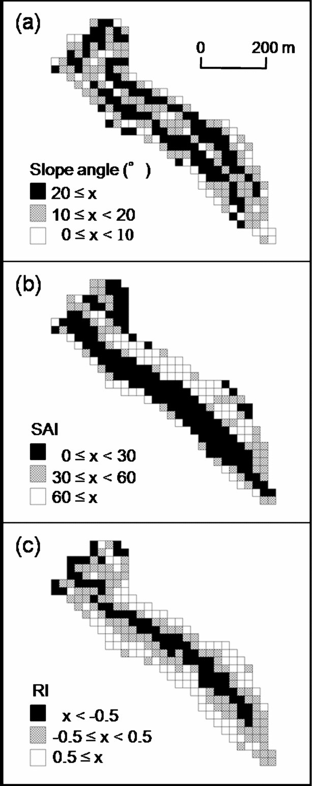
The three topographic parameters varied spatially (Figure 2). The median values (range) of slope angle, SAI and RI in the cells were 17° (1–34°), 27.8 (0.6–97.8), and 0.1 (−1.6 to 1.5), respectively. There were no significant correlations between slope angle and SAI, and between SAI and RI (Pearson's product-moment correlation test: r = 0.09, P = 0.17; r = 0.06, P = 0.36, respectively). There was a significant negative correlation between slope angle and RI, but the correlation was weak (Pearson's product-moment correlation test: r = −0.14, P < 0.05).
Spatial variation of topographic parameters in the plot. Slope angle (a), Slope aspect index (SAI) (b), Relief index (RI) (c).
Liana community structure
A total of 930 stems ≥ 2 cm in diameter was recorded in the study plot (16.0625 ha) (Table 1). The basal area (BA) of lianas in the study plot was 1.07 m2. Lianas were found in 178 of 257 cells. Among the cells in which lianas were found, stem density and BA of lianas ranged from 16 to 592 stems ha−1, and from 0.09 to 1.47 m2 ha−1, respectively.
Stem density, basal area (BA) and climbing type of all liana species with > 2 cm stem diameter found in the study watershed (16.0625 ha). TW = twining climber, RC = root climber, TD = tendril climber, SC = scrambling climber
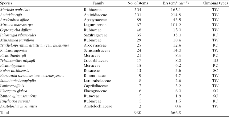
Lianas recorded represented 20 species from 15 families. The most abundant species in number of stems was Morinda umbellata (Rubiaceae), followed by Actinidia rufa (Actinidiaceae) and Anodendron affine (Apocynaceae). In BA, dominant species were A. rufa followed by M. umbellata and Mucuna macrocarpa (Leguminosae). Four climbing types were recorded. Twining was the dominant climbing type and represented 55% of all species, and 85% of all stems. Root climbing was the second dominant climbing type, and represented 25% of all species, and 11% of all stems. Scrambling climbers represented 15% of all species, and 3% of all stems. Tendril climbers represented 5% of all species, and 2% of all stems.
Relationship between topography and distribution
The probability of occurrence of all liana species combined was positively and significantly related to slope angle (Figure 3). The probability of occurrence was 44% in the cell with the minimum slope angle (1°) and 88% in the cell with the maximum slope angle (34°). The probability of occurrence of all liana species combined was negatively and significantly related to RI. The probability of occurrence was 96% in the cell with the minimum RI value (–1.6) and 26% in the cell with the maximum RI value (1.5). RI contributed to a decrease in deviance more than slope angle. SAI did not contribute to a decrease in deviance.
Relationships between each topographic factor and probability of occurrence of all liana species analysed using GLM with binomial distribution. Solid line on each figure represents variation of the probability of occurrence along each topographic factor. Open circles in the figures indicate cell data (i.e. 1 = presence of lianas; 0 = absence). Slope angle (probability of occurrence = 1/(1 + exp(–(−0.32 + 0.07 × slope angle))): Decrement of deviance from null model = 12; significant at 95% confidence interval) (a). Slope aspect index (SAI) (probability of occurrence = 1/(1 + exp(–(0.56 + 0.01 × SAI))): Decrement of deviance from null model = 2; not significant at 95% confidence interval) (b). Relief index (RI) (probability of occurrence = 1/(1 + exp(–(0.99 + (−1.36) × RI))): Decrement of deviance from null model = 41; significant at 95% confidence interval) (c).

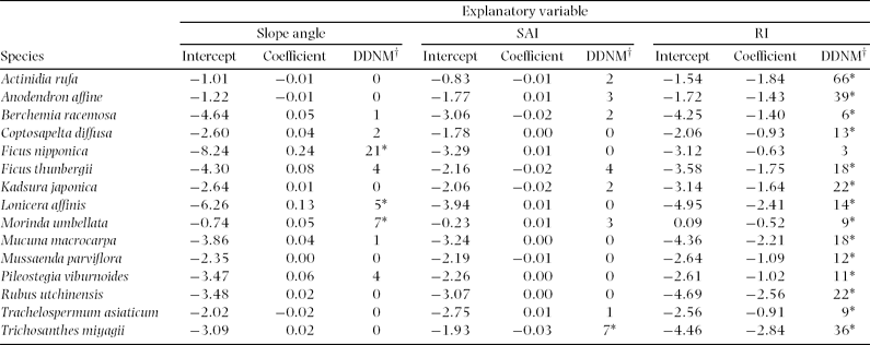
For species-level analyses, Stauntonia hexaphylla, Elaeagnus glabra, Zanthoxylum scandens, Psychotria serpens and Aristolochia liukiuensis were excluded, because they were recorded in less than five cells. At the species level, slope angle positively affected distribution of three species, Ficus nipponica, M. umbellata and Lonicera affinis, out of 15 species (Table 2). SAI positively affected distribution of Trichosanthes miyagii. Distributions of all species excluding F. sarmentosa were negatively related to RI.
Relationships between distribution of each species and each topographic factor; slope angle, slope aspect index (SAI), and relief index (RI). Data were analysed using a generalized linear model with binomial distribution. Asterisks indicate that difference in deviance from that of null model (DDNM†) is significant at 95% confidence interval.
Relationship between topography and abundance
Slope angle and RI were negatively related to stem density of all liana stems (Figure 4). Stem densities were 91 stems ha−1 in the cell with minimum slope angle (1°) and 77 stems ha−1 in the cell with maximum slope angle (34°). Stem densities on the GLM model were 227 stems ha−1 in the cell with minimum RI value (−1.6) and 17 stems ha−1 in the cell with maximum RI value (1.5). RI contributed to a decrease in deviance more than slope angle. There was no significant relationship between SAI and stem density.
Relationships between each topographic factor and stem density of total lianas analysed using GLM with Poisson distribution. Solid line on each figure represents variation of stem density along each topographic factor. Dots in the figures indicate the cells. Slope angle (stem density = exp(4.52 + (−0.005) × slope angle)): Decrement of deviance from null model = 20; significant at 95% confidence interval) (a). Slope aspect index (SAI)(stem density = exp(4.46 + (−0.001) × SAI): Decrement of deviance from null model = 0; not significant at 95% confidence interval) (b). Relief index (RI) (stem density = exp(4.08 + (−0.841) × RI): Decrement of deviance from null model = 4926; significant at 95% confidence interval) (c).

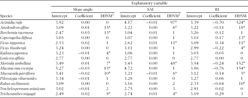
At the species level, slope angle positively affected stem density of four species and negatively affected stem density of three species (Table 3). SAI positively affected stem density of four species and negatively affected stem density of two species. RI positively affected stem density of three species and negatively affected six species.
Relationships between stem density of each species and each topographic factor; slope angle, slope aspect index (SAI), and relief index (RI). Data were analysed using a generalized linear model with Poisson distribution. Asterisks indicate that difference in deviance from that of null model (DDNM) is significant at 95% confidence interval.
DISCUSSION
In this study, we found that abundance of lianas was high in concave sites and distribution of most liana species was biased toward concave sites in the watershed. Putz & Chai (Reference PUTZ and CHAI1987) also reported that abundance of lianas was more than two-fold greater at a valley site than at a hill-top site. The spatial pattern could be explained partly by the below-ground resource gradient. Concave topography is typified by high soil water content and nutrient availability, and vice versa for convex topography (Gessler et al. Reference GESSLER, CHADWICK, CHARMRAN, ALTHOUSE and HOLMES2000, Roy & Singh Reference ROY and SINGH1994). Gradient of water availability could be a determinant of distribution and abundance of lianas (Ibarra-Manríquez & Martínez-Ramos Reference IBARRA-MANRÍQUEZ and MARTÍNEZ-RAMOS2002, Teramura et al. Reference TERAMURA, GOLD, FORSETH, Putz and Mooney1991). It has been suggested that soil fertility is positively correlated with liana abundance (Laurance et al. Reference LAURANCE, PÉREZ-SALICRUP, DELAMÔNICA, FEARNSIDE, D'ANGELO, JEROZOLINSKI, POHL and LOVEJOY2001, Putz & Chai Reference PUTZ and CHAI1987). Tateno & Takeda (Reference TATENO and TAKEDA2003) suggested that competition for light could be intensified in lower slopes with rich below-ground resources. In that situation, lianas (and herbaceous climbers) may have an advantage in competing for light with their strategies such as low cost of support tissue (Teramura et al. Reference TERAMURA, GOLD, FORSETH, Putz and Mooney1991) and horizontal elongation of stolons to reach better environments (Peñalosa Reference PEÑALOSA1983, Reference PEÑALOSA1984; Sakai et al. Reference SAKAI, NOMIYA and SUZUKI2002). In contrast to valleys, water and/or nutrient availability could limit plant distribution on ridges (Kubota et al. Reference KUBOTA, MURATA and KIKUZAWA2004, Tateno & Takeda Reference TATENO and TAKEDA2003).
Disturbance regimes also change with topography. Convex sites with gentle slopes are relatively stable in terms of surface soil, while small canopy gaps are frequently formed by typhoons or strong winds in the Okinawa forest (Enoki Reference ENOKI2003, Kubota et al. Reference KUBOTA, MURATA and KIKUZAWA2004). Our results suggest that canopy disturbance is not a primary factor in determining distribution and abundance of lianas in the watershed, although canopy disturbance could be an important factor affecting abundance of lianas within a tropical forest (Putz Reference PUTZ1984). Concave sites with steep slopes are unstable in terms of surface soil, and soil disturbances such as landslides occur frequently (Hunter & Parker Reference HUNTER and PARKER1993, Nagamatsu & Miura Reference NAGAMATSU and MIURA1997). Three species, Ficus nipponica, M. umbellata and Lonicera affinis, showed a positive relationship between distribution and slope angle. These species might depend on soil disturbance for regeneration, as Enoki (Reference ENOKI2003) suggested for tree species in the subtropical forest.
Wind stress could also constrain distribution of lianas on the ridges. Generally ridges tend to have higher wind exposure than valleys (Webb et al. Reference WEBB, STANFIELD and JENSEN1999). Wind increases transpiration accompanied by leaf water stress (Grace & Russell Reference GRACE and RUSSELL1982). Slope aspect can influence wind regimes and influence distribution of vegetation (Burke et al. Reference BURKE, REINERS and OLSON1989). The study watershed faces to windward of the north-west monsoon. One of the possible reasons for lack of a significant relationship between lianas and slope aspect may be due to the spatial resolution used in the study.
Distribution of lianas was biased toward valley areas. This was in contrast to the distribution of standing trees in the Okinawa forest. Stem density and species diversity of standing trees are generally high on the ridges or upper slopes in the forest on Okinawa (Enoki Reference ENOKI2003, Kubota et al. Reference KUBOTA, MURATA and KIKUZAWA2004). Most of the tree species distributed on ridges in subtropical forests are wind- and/or drought-tolerant species (Kubota et al. Reference KUBOTA, MURATA and KIKUZAWA2004). Enoki (Reference ENOKI2003) suggested that the low density of standing trees in valley areas is a result of soil disturbance. In the present study, the distribution pattern of lianas from ridge to valley might reflect the susceptibility to water stress and tolerance to soil disturbance. Our results suggested that distribution and abundance of lianas are strongly affected by topography. Lianas tend to be distributed in sites with more water and nutrients, which are formed by relief in the Okinawa subtropical broad-leaved forest. Further study is needed to clarify mechanisms by which topographic factors affect distribution and abundance of lianas observed in the present study.
ACKNOWLEDGEMENTS
We thank our field assistants, Masaru Mukouda and Yasuhiko Nakahara, students of the Kagoshima University and Daisuke Nanki, a student of the University of the Ryukyus. This study was supported by grants from the Ministry of Education, Culture, Sports, Science and Technology, Japan, and Okinawa Prefectural Government.



