1. Introduction
The dynamics of liquid cones is of interest because conical interfaces develop both in the late stages of pinch-off of cylindrical jets (Peregrine, Shoker & Symon Reference Peregrine, Shoker and Symon1990; Shi, Brenner & Nagel Reference Shi, Brenner and Nagel1994) and when drops are in the presence of electric fields (de la Mora Reference de la Mora2007). Recent experiments have demonstrated that in the presence of electric fields, the interface of pairs of water drops can deform so that they connect with a double-cone geometry (figure 1) and, depending on the physical parameters, the drops will either coalesce or recoil (Bird et al. Reference Bird, Ristenpart, Belmonte and Stone2009; Ristenpart et al. Reference Ristenpart, Bird, Belmonte, Dollar and Stone2009; Thiam, Bremond & Bibette Reference Thiam, Bremond and Bibette2009). The resulting transition from coalescence to recoil at impact has numerous implications, including the coalescence of electrified raindrops in thunderstorm formation (Latham Reference Latham1969), the removal of water from oil in the petroleum industry (Eow et al. Reference Eow, Ghadiri, Sharif and Williams2001; Ristenpart et al. Reference Ristenpart, Bird, Belmonte, Dollar and Stone2009), the stability of pH-sensitive emulsions (Liu et al. Reference Liu, Seiffert, Thiele, Abate, Weitz and Richtering2012), and the coalescence of Pickering emulsions by electric fields (Chen et al. Reference Chen, Tan, Chen, Huang, Wen and Xu2013). To date, the underlying physics of this transition are not completely understood, although it is believed to arise from the conical geometry rather than from electrical interactions in the flow. Models have been developed to rationalize this transition between coalescence and recoil based on cone angle (Bird et al. Reference Bird, Ristenpart, Belmonte and Stone2009; Ristenpart et al. Reference Ristenpart, Bird, Belmonte, Dollar and Stone2009; Helmensdorfer Reference Helmensdorfer2012); however, there is a lack of consensus surrounding these models, as each neglects key elements of the flow. In the current paper, we use high-resolution numerical simulations to explore how these conical drops coalesce. In addition, this work demonstrates that conditions initially favouring coalescence can dynamically reverse, leading to drop pinch-off and recoil.
Initial geometry of contacting conical droplets. (a) Two liquid drops with radius of curvature
 $R$
(grey) are surrounded by air (white) and are joined with a hyperboloid bridge. (b) At intermediate scales, the bridge appears conical with polar angle
 ${\it\theta}$
. (c) Higher magnification reveals that the two droplets are connected with a bridge with radius
 $r_{0}$
. (d) Experimental observation of the conical liquid bridge formed when two water drops are separated by 500 V.

The coalescence or pinch-off of liquid bridges can often be rationalized by the sign of the mean curvature of the interface, as this curvature is related to the capillary pressure (de Gennes, Brochard-Wyart & Quere Reference de Gennes, Brochard-Wyart and Quere2004). For example, when two spherical water drops contact, the bridge connecting the spheres has a negative mean curvature (there is a much smaller positive curvature around the bridge than the negative curvature along the bridge), leading to a pressure drop in the bridge that draws in liquid and drives coalescence (Eggers, Lister & Stone Reference Eggers, Lister and Stone1999; Wu, Cubaud & Ho Reference Wu, Cubaud and Ho2004; Thoroddsen, Takehara & Etoh Reference Thoroddsen, Takehara and Etoh2005). In contrast, when a jet of water initially breaks up from the Rayleigh–Plateau instability, the bridge formed has a larger positive curvature around the bridge than the negative curvature along the bridge, leading to a higher pressure in the bridge region that pinches off the liquid (Eggers Reference Eggers1997). However, when the two principal curvatures are estimated to be opposite and similar in magnitude, it is not immediately obvious whether the drop will coalesce or pinch off. A conical liquid bridge between two drops (figure 1) is an example of such a geometry.
Previous models exploring the critical angle at which the conical drops either coalesce or pinch off have made assumptions about key physical elements. For example, the scaling argument in Ristenpart et al. (Reference Ristenpart, Bird, Belmonte, Dollar and Stone2009) recognized the competing principal curvatures, but did not explicitly model the curvatures in the bridge region. The analytic argument in Bird et al. (Reference Bird, Ristenpart, Belmonte and Stone2009) assumed that the largest deformations would occur in a bridge region and that these would be self-similar as the drops coalesced. The self-similar shape of this bridge region was estimated to be the profile that minimized surface area while constrained to connect the bridge to the surrounding cones and conserved volume. Thus the bridge shape was calculated independently from any of the dynamics in the surrounding cones and therefore neglected inertial effects, even though inertia was regulating the bridge dimensions. A more recent model was developed based on mean curvature flow (Helmensdorfer Reference Helmensdorfer2012; Helmensdorfer & Topping Reference Helmensdorfer and Topping2013), yet it is unclear how well this approach models the underlying physics since mass and momentum are not necessarily conserved. It is also noteworthy that the absence of inertia in mean curvature flow prevents the self-similar dynamics that often appear in similar geometries (Barenblatt & Zel’Dovich Reference Barenblatt and Zel’Dovich1972; Keller & Miksis Reference Keller and Miksis1983).
A natural approach to addressing these model limitations would be to solve the inviscid self-similar equations formulated by Keller & Miksis (Reference Keller and Miksis1983). Specifically, in geometries where there is no characteristic length scale, such as wedges and cones, the inviscid dynamics (potential flow) can be simplified and solved in self-similar variables. The approach has been used to model the pinch-off of inviscid bridges between two far-field slender cones (Brenner et al. Reference Brenner, Eggers, Joseph, Nagel and Shi1997; Day, Hinch & Lister Reference Day, Hinch and Lister1998; Leppinen & Lister Reference Leppinen and Lister2003), as well as recoiling dynamics of wedges (Keller & Miksis Reference Keller and Miksis1983; Lawrie Reference Lawrie1990) and cones (Billingham Reference Billingham1999; Sierou & Lister Reference Sierou and Lister2004) that would occur after the bridge had pinched off. The coalescence of liquid wedges has also been simulated using these inviscid self-similar equations (Keller, Milewski & Vanden-Broeck Reference Keller, Milewski and Vanden-Broeck2000); it appears that two-dimensional wedges coalesce for any and all angles. It is important to note that none of these previous studies investigated the coalescence dynamics of two liquid cones.
In the current paper, we numerically investigate the coalescence dynamics for two low-viscosity conical droplets surrounded by an even less viscous gas. A challenge with solving directly for a self-similar solution is that, even in a conical geometry, self-similar solutions of the first kind may not exist. For example, the self-similarity might break-down due to a self-intersecting boundary (Duchemin, Eggers & Josserand Reference Duchemin, Eggers and Josserand2003; Billingham & King Reference Billingham and King2005), or alternatively memory of the initial conditions might lead to anomalous scaling exponents (Burton & Taborek Reference Burton and Taborek2007). To allow for all possible dynamics, we choose to solve the full Navier–Stokes equations using a volume-of-fluid technique. Specifically, we include both the inertia and viscosity of the liquid and the surrounding gas, as well as the surface tension and non-conical aspects of the geometry. By including all of these parameters, we are able to confirm that certain aspects indeed have negligible effects. We aim to use the simulation results to reconcile differences in the previous conical coalescence models, as well as explore the extent to which the solutions exhibit self-similar dynamics at intermediate length and time scales.
2. Numerical approach
For conical drops to coalesce, they need to be connected at some small scale. We also want to ensure that the boundary conditions at the point where the cone joins the spherical droplet are appropriate. The geometry that we are modelling consists of two spheres smoothly connected to a hyperboloid bridge (figure 1). At the largest scale, the spheres have radius
 $R$
and are surrounded by a gas in a
 $4R\times 6R$
domain (figure 1
a). When the tangent of the spheres approaches a chosen angle
 ${\it\theta}$
off the axis of symmetry (the cone half-angle), the geometry smoothly transitions into a hyperbolic surface expressed by
 $$\begin{eqnarray}\left(\frac{r}{r_{0}}+\frac{\tan ^{2}{\it\theta}}{c}-1\right)^{2}-\tan ^{2}{\it\theta}\left(\frac{z}{r_{0}}\right)^{2}=\frac{\tan ^{4}{\it\theta}}{c^{2}},\end{eqnarray}$$
where
 $r$
and
 $z$
represent the axisymmetric coordinates,
 $r_{0}$
the initial bridge radius (figure 1
c), and
 $c$
is a constant that is used to control the sign of the bridge curvature. At the transition point between the spherical droplet and hyperbolic region, the profile and profile slope are continuous and the curvature is discontinuous. Here the cone half-angle
 ${\it\theta}$
refers to the angle from the
 $z$
axis. The family of hyperbolic surfaces generated by (2.1) was selected because it has two important characteristics. First, the mean curvature at the centre of the hyperbola is
 $\mathscr{H}(c)=(1/r_{0}-c/r_{0})/2$
, and therefore identical for all values of
 ${\it\theta}$
for a fixed value of
 $c$
(figure 1
c). The mean curvature is relevant because its value determines the pressure difference, or capillary pressure, across the interface following
 ${\rm\Delta}p=2{\it\gamma}\mathscr{H}_{0}$
, where
 ${\it\gamma}$
is the surface tension. Therefore if
 $c>1$
, then the initial mean curvature at
 $z=0$
is negative and there is lower pressure in the bridge than in the surrounding drop, leading to flow into the bridge region and permitting coalescence. The second important characteristic is that at an intermediate scale, smaller than the radius of the drops, but sufficiently far from the origin (figure 1
b), the hyperboloid takes the shape of a double cone with
 $r=(\tan {\it\theta})z$
. At the largest scales, the cone is matched to the line tangent to a spherical droplet (figure 1
a). Provided that
 $r_{0}\ll R$
for a given initial angle
 ${\it\theta}$
and droplet radius
 $R$
, the droplet centre is located along the axis of symmetry at
 $$\begin{eqnarray}z_{d}=\pm R\,\text{cosec}\,{\it\theta}.\end{eqnarray}$$
The point where the cones join the droplets,
 $z_{i}$
, occurs at
 $$\begin{eqnarray}z_{i}=\pm R(\text{cosec}\,{\it\theta}-\sin {\it\theta}).\end{eqnarray}$$
It should be noted that we are interested in the coalescence of conical interfaces (figure 1 b). The non-conical aspects of the imposed geometry are added to avoid singularities and to connect the conical geometry with physically plausible, albeit approximate, boundary conditions.
Once the initial geometry has been established, the coalescence dynamics of the system are then solved numerically (figure 2). Due to the symmetry of the problem, the axisymmetric Navier–Stokes equations are solved instead of the fully three-dimensional system. The computations employ the open source software Gerris (Popinet Reference Popinet2003), which simulates the incompressible multi-phase Navier–Stokes equations using a volume-of-fluid technique. Gerris is chosen for ease of parallelization and its ability to adaptively represent physical scales spanning several orders of magnitude (Thoraval et al. Reference Thoraval, Takehara, Etoh, Popinet, Ray, Josserand, Zaleski and Thoroddsen2012). In dimensional form, Gerris solves the Navier–Stokes equations modified to include surface tension at fluid interfaces:
 $$\begin{eqnarray}{\it\rho}\frac{\text{D}\boldsymbol{u}}{\text{D}t}=-\boldsymbol{{\rm\nabla}}p+\boldsymbol{{\rm\nabla}}\boldsymbol{\cdot }{\it\mu}(\boldsymbol{{\rm\nabla}}\boldsymbol{u}+\boldsymbol{{\rm\nabla}}\boldsymbol{u}^{\text{T}})+2\mathscr{H}{\it\gamma}{\it\delta}_{s}\boldsymbol{ n },\end{eqnarray}$$
where
 $\boldsymbol{u}$
is the fluid velocity,
 ${\it\rho}$
the density,
 $p$
the pressure,
 ${\it\mu}$
viscosity,
 $\boldsymbol{n}$
the normal to the gas–liquid interface, and
 ${\it\delta}_{s}$
a Dirac delta function on the interface. Equation (2.4) can be non-dimensionalized by dividing through by
 ${\it\gamma}/L^{2}$
, where
 $L$
is the characteristic length scale. It is apparent that this introduces a characteristic time
 ${\it\tau}_{c}=\sqrt{{\it\rho}L^{3}/{\it\gamma}}$
and velocity
 $u_{c}=L/{\it\tau}_{c}$
, as well as the dimensionless Ohnesorge number
 $\mathit{Oh}={\it\mu}/\sqrt{{\it\rho}{\it\gamma}L}$
. Additionally, the dimensionless density
 ${\it\rho}_{r}={\it\rho}_{g}/{\it\rho}_{\ell }$
and viscosity
 ${\it\mu}_{r}={\it\mu}_{g}/{\it\mu}_{\ell }$
ratios are used to characterize the two fluids, where the subscripts
 $g$
and
 $\ell$
denote gas and liquid phases, respectively. Here the density ratio, viscosity ratio, and Ohnesorge number are set to
 ${\it\rho}_{r}=1.2\times 10^{-3}$
,
 ${\it\mu}_{r}=1.8\times 10^{-2}$
, and
 $\mathit{Oh}=2.7\times 10^{-3}$
, consistent with a water droplet of radius
 $R=2~\text{mm}$
in air. A final dimensionless ratio
 $R/r_{0}$
sets the range of physical scales over which the simulation is carried out. We choose this ratio to be as large as physically reasonable with
 $R/r_{0}=10^{4}$
such that smallest length scale is
 $r_{0}=0.2~{\rm\mu}\text{m}$
. The motivation behind this selection is to neglect gravitational effects at
 $R$
and molecular interactions at
 $r_{0}$
. Our results should adequately approximate the dynamics of any size of drops with length scales within this regime.
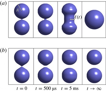
Numerical results highlight two different outcomes based on the cone angle
 ${\it\theta}$
relative to a critical angle
 ${\it\theta}_{c}$
. (a) Snapshots of the drop pair at different times
 $t$
illustrate that two connected drops with cone angle
 ${\it\theta}=1.2$
will coalesce into one drop. (b) Snapshots reveal that a drop pair with cone angle
 ${\it\theta}=1.0$
will follow a different trajectory and result in two separated drops. The fluid parameters are selected to model water droplets in air with radius
 $R=2~\text{mm}$
and the initial mean curvature
 $\mathscr{H}_{0}(c=3)=-1/r_{0}$
.

Simulations begin with two symmetric droplets connected and initially at rest; capillary forces drive the subsequent motion. Each simulation is carried out until the initially connected cone has completely retracted in the case of non-coalescence, or the two droplets coalesce completely into a single droplet.
3. Results and discussion
Results use the convention of angle described in Sierou & Lister (Reference Sierou and Lister2004), unless otherwise noted, where increasing or decreasing
 ${\it\theta}$
results in ‘blunter’ or ‘sharper’ cones, respectively. The resulting dynamics are illustrated in figure 2 for initially coalescing cones with mean curvature
 $\mathscr{H}_{0}(c=3)=-1/r_{0}$
. When the bridge connecting the drop pair is blunter than a critical angle (
 ${\it\theta}>{\it\theta}_{c}$
), snapshots at various times
 $t$
illustrate that the drop pair eventually coalesces into a single drop (figure 2
a). However, when the bridge connecting the drop pair is sharper than a critical cone angle (
 ${\it\theta}<{\it\theta}_{c}$
), the bridge quickly pinches off, resulting in a pair of recoiling drops (figure 2
b). As far as we are aware, these are the first numerical simulations that include both inertia and surface tension to demonstrate that drop pairs connected by conical bridges coalesce or recoil.
3.1. Self-similar dynamics
The dynamics of coalescence can be quantified by tracking the bridge radius
 $\ell (t)$
. To generalize the results, it is often helpful to cast them in physically appropriate non-dimensional variables. It is natural to normalize
 $\ell (t)$
by either
 $R$
or
 $r_{0}$
, depending on the scale of interest. In these simulations, we have selected an Ohnesorge number based on the largest scale corresponding to the droplet radius
 $R$
to be
 $\mathit{Oh}=2.7\times 10^{-3}$
, and
 $\mathit{Oh}=0.27$
at the smallest scale
 $r_{0}$
. Thus
 $\mathit{Oh}<1$
at all length scales in this problem, indicating that inertia is more important than viscosity at all scales, and that time would be appropriately non-dimensionalized by an inertial–capillary time scale
 $\sqrt{{\it\rho}_{\ell }L^{3}/{\it\gamma}}$
, where
 $L$
is the characteristic length scale.
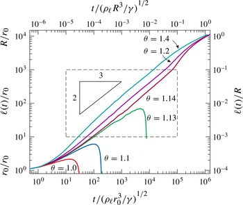
The motion
 $\ell (t)$
is plotted in log coordinates for various cone angles
 ${\it\theta}$
(figure 3). Initially, all the curves start at
 $\ell (0)/r_{0}=1$
and follow the same trajectory because the different drop pairs have the same initial mean curvature at the centre of the bridge and coalesce at the same rate. As time progresses, the effects of
 ${\it\theta}$
become more pronounced, and the curves deviate. For drops with
 ${\it\theta}\leqslant 1.13$
, the effect of the cone angle not only reduces the coalescence, but completely reverses it, leading to pinch-off. For drops with
 ${\it\theta}\geqslant 1.14$
, the curves become straight and parallel in an intermediate regime (dashed box in figure 3) before re-converging as
 $\ell (t)$
approaches
 $R$
.
Evolution of the bridge radius
 $\ell (t)$
in non-dimensionalized variables for six cone angles each with initial mean curvature
 $\mathscr{H}_{0}(c=3)=-1/r_{0}$
. For
 ${\it\theta}\leqslant 1.13$
, the two drops initially coalesce and then recoil. For
 ${\it\theta}\geqslant 1.14$
the two droplets coalesce. The dashed box highlights the intermediate time and space scales where
 $r_{0}\ll \ell (t)\ll R$
. It is in this intermediate regime where the liquid can be approximated as cones (figure 1
b).

These results highlight the separation of scales in figure 1. At both the smallest and largest scales (figure 1
a,c), the cone angle has a small influence on the geometry relative to the dominant length scale (
 $R$
and
 $r_{0}$
respectively), and in these regimes curves for various
 ${\it\theta}$
nearly collapse (figure 3). In contrast, at the intermediate scale, (figure 1
b), there is no dominant length scale, and in this regime the curves vary with
 ${\it\theta}$
and exhibit a power-law growth with an expected exponent of
 $2/3$
with small deviations over a finite range of scales. This exponent is noteworthy because the
 $2/3$
value allows the bridge radius to be expressed as
 $\ell (t)\sim (t^{2}{\it\gamma}/{\it\rho}_{\ell })^{1/3}$
, which is independent of any length scale. Had the inviscid self-similar equations been solved instead, a scaling with the
 $2/3$
exponent would be expected by construction (Keller & Miksis Reference Keller and Miksis1983; Sierou & Lister Reference Sierou and Lister2004). However, the present simulations include various length scales, which suggests that the dynamics include the existence of self-similar solutions as intermediate asymptotics (Barenblatt & Zel’Dovich Reference Barenblatt and Zel’Dovich1972). Specifically, the precise shape of the initial geometry on the scale of
 $r_{0}$
and
 $R$
has a negligible effect on the dynamics in the intermediate regime.
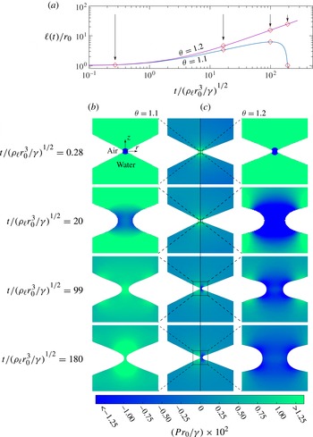
Because we are solving the full equations of motion rather than the self-similar inviscid equations, we can investigate the initial non-self-similar dynamics (figure 4). The initial bridge dynamics
 $\ell (t)$
for droplets with initial angles of
 ${\it\theta}=1.2>{\it\theta}_{c}$
and
 ${\it\theta}=1.1<{\it\theta}_{c}$
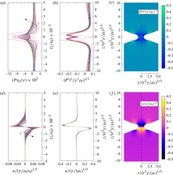
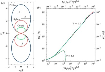
are shown in figure 4(a). The corresponding pressure fields are shown for the non-coalescing and coalescing droplets in figures 4(b) and 4(c), respectively. At the initial bridge scale
 $r_{0}$
, a natural non-dimensionalization of pressures is
 $Pr_{0}/{\it\gamma}$
. At the earliest times, the pressure fields are almost entirely generated by local mean curvatures. The pressure fields for both
 ${\it\theta}=1.2$
and
 ${\it\theta}=1.1$
are nearly identical when
 $t/({\it\rho}_{\ell }r_{0}^{3}/{\it\gamma})^{1/2}=0.28$
, with a strong negative pressure region initially drawing fluid into the bridge region. However, the interface dynamics quickly begin to be affected by the cone angle. At
 $t/({\it\rho}_{\ell }r_{0}^{3}/{\it\gamma})^{1/2}=20$
the bridge regions have increased in diameter for both
 ${\it\theta}=1.1$
and
 ${\it\theta}=1.2$
. At this point the pressure at the centre of the bridge is
 $Pr_{0}/{\it\gamma}\approx 0$
for
 ${\it\theta}=1.1$
while the centre of the bridge for
 ${\it\theta}=1.2$
maintains a negative pressure. This transition in the sign of the pressure is reflected by the inflection point in
 $\ell (t)$
for
 ${\it\theta}=1.1$
(figure 4
a). Eventually the pressure for
 ${\it\theta}=1.1$
becomes positive (figure 4
b,
 $t/({\it\rho}_{\ell }r_{0}^{3}/{\it\gamma})^{1/2}=99$
), causing the collapse of the bridge region. The droplet pair with
 ${\it\theta}=1.2$
is able to maintain the negative mean curvature in the bridge region, eventually continuing on towards self-similar coalescence (figure 4
c,
 $t/({\it\rho}_{\ell }r_{0}^{3}/{\it\gamma})^{1/2}=180$
).
Initial dynamics are shown for coalescing and non-coalescing droplet pairs. (a) Bridge radius
 $\ell (t)$
is shown for angles
 ${\it\theta}=1.1<{\it\theta}_{c}$
and
 ${\it\theta}=1.2>{\it\theta}_{c}$
and initial non-dimensional curvature
 $\mathscr{H}_{0}(c=3)r_{0}=-1$
. (b,c) Pressure fields, for
 ${\it\theta}=1.1$
and
 $1.2$
respectively, with appropriate non-dimensional scaling
 $Pr_{0}/{\it\gamma}$
in the bridge region driving the interface are shown as time progresses. Images in the left and right columns correspond to a scaled up view of the small boxed areas shown in the middle column. Views of the non-coalescing and coalescing droplet pairs correspond to the left and right halves of the middle column images, respectively. Initially, both fields are driven by identical initial curvatures. A short time later the pressure in the non-coalescing bridge becomes positive, driving fluid out of the region leading to break-up. For the coalescing droplets pressure remains negative until the pair completely merge.

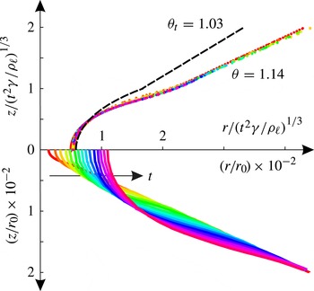
To illustrate that intermediate dynamics are indeed self-similar, profiles of the coalescing bridge are plotted at different intermediate times for
 ${\it\theta}=1.14$
(figure 5). When the spatial coordinates (
 $r,z$
) are normalized by
 $r_{0}$
, the bridge expands with time as it coalesces. However, when the spatial coordinates are normalized by the self-similar length scale
 $(t^{2}{\it\gamma}/{\it\rho}_{\ell })^{1/3}$
, the curves collapse almost perfectly onto a single coalescing profile.
Free surface of coalescing drops near the critical angle
 ${\it\theta}=1.14$
and initial mean curvature
 $\mathscr{H}_{0}(c=3)=-1/r_{0}$
for the range of intermediate times
 $t/({\it\rho}_{\ell }r_{0}^{3}/{\it\gamma})^{1/2}=10^{2}$
to
 $10^{4}$
. Lower half: spatial variables
 $(r,z)$
depict how the profile evolves with time; upper half: rescaled variables demonstrate that the profile in the intermediate regime is self-similar. Dashed line corresponds to a previous analytic approximation to self-similar shape near the transition angle, calculated to be near
 ${\it\theta}\approx 1.03$
(Bird et al.
Reference Bird, Ristenpart, Belmonte and Stone2009).

Because this profile is near
 ${\it\theta}_{c}$
, it can be contrasted with a previous estimate for this shape (dashed line in figure 5, Bird et al.
Reference Bird, Ristenpart, Belmonte and Stone2009). The previous model split the bridge into perturbed and non-perturbed regions that connected at the point
 $z/(t^{2}{\it\gamma}/{\it\rho}_{\ell })^{1/3}=1$
, leading to a kink of non-monotonic curvature in the boundary. The perturbed region neglects the fluid inertia and is assumed to minimize surface energy while constraining volume. This assumption leads to a constant-mean curvature surface with a uniform bridge pressure. In this model, coalescence is assumed to require flow into the perturbed region driven by a negative capillary pressure in the bridge. Thus the transition angle between continued coalescence and recoil is assumed to occur when the capillary pressure in the bridge is zero. If the liquid mass in the bridge is conserved, this transition angle occurs when the far-field cone angle is approximately
 ${\it\theta}_{t}=1.03$
.
The present simulations demonstrate that a self-similar approximation is appropriate and also illustrate the existence of non-monotonic curvature in the profile, albeit one that is smooth (figure 5). Yet, the curves demonstrate that the precise shape of the bridge is somewhat different than previously modelled, and the critical angle
 ${\it\theta}_{c}$
is between 1.13 and 1.14, rather than the previously modelled value
 ${\it\theta}_{t}=1.03$
.
Given the success of self-similar variables in collapsing the free-surface profiles in figure 5, it is natural to inquire how the pressure field develops and varies as it enters this intermediate regime. Our simulations show that the highest and lowest pressures are localized to the bridge region at early times (figure 4). Additionally, there is significant spatial variability in the pressure field within this region. For the coalescing droplet pair with
 ${\it\theta}=1.2$
(figure 4
c), the pressure along the axis of symmetry (
 $r=0$
) goes from a negative pressure at the origin to an even lower pressure at the edge of the bridge region and then to a higher pressure outside this region. The magnitude of these pressure variations decreases with time. To investigate this pressure behaviour in the intermediate regime, we have plotted values of pressure along the axis of symmetry over
 $z=-100r_{0}$
to
 $100r_{0}$
for the coalescing droplet pair with angle
 ${\it\theta}=1.2$
(figure 6
a). Results are shown for times
 $t/({\it\rho}_{\ell }r_{0}^{3}/{\it\gamma})^{1/2}=10^{2}$
to
 $10^{3}$
, which overlaps with the times in figure 4 and corresponds to the start of the intermediate self-similar regime identified in figure 3.
Pressure and vertical velocity profiles during coalescence in the intermediate regime for
 ${\it\theta}=1.2$
and initial non-dimensional mean curvature
 $\mathscr{H}_{0}(c=3)r_{0}=-1$
over one decade of time spanning from
 $t/({\it\rho}_{\ell }r_{0}^{3}/{\it\gamma})^{1/2}=10^{2}$
to
 $10^{3}$
. (a) Magnitude of pressure depends on the axial position and decreases with time. (b) When scaled by self-similar spatial variables, the pressure collapses onto a single curve. (c) The same self-similar pressure is shown over the entire bridge region. (d) The magnitude of vertical velocity also depends on axial position and decreases with time. (e) Rescaling these velocity profiles with self-similar variables leads to a single curve. ( f) The same self-similar vertical velocity is shown over the entire bridge.

Figure 6 illuminates the effect of cone angle on the pressure field driving the initial bridge trajectories towards coalescence or break-up. For droplet pairs with cone angle
 ${\it\theta}>{\it\theta}_{c}$
the pressure field sustains flow into the bridge region throughout intermediate times. Given that the pressure fields are driven by mean curvature of the fluid–air interface, and that the interface enters an intermediate self-similar regime, it is expected that the pressure and velocity fields are also self-similar near the bridge region.
As time progresses and the bridge radius increases in size, the magnitude of the negative pressure in the liquid bridge decreases. The values and trends of pressure in figure 6(a) are consistent with those in figure 4(c), recognizing that some of the pressure values in figure 4(c) go beyond the scale-bar limits at early times. When the pressure curves from figure 6(a) are rescaled with appropriate self-similar variables, they nearly collapse onto a single self-similar curve (figure 6
b). The corresponding self-similar pressure field is shown in figure 6(c), where the axis of symmetry is represented by the dotted line. The domain extends over
 $z/(t^{2}{\it\gamma}/{\it\rho}_{\ell })^{1/3}$
from
 $-10$
to 10 and
 $r/(t^{2}{\it\gamma}/{\it\rho}_{\ell })^{1/3}$
from 0 to 5. The vertical scale corresponding to the self-similar variable
 $z/(t^{2}{\it\gamma}/{\it\rho}_{\ell })^{1/3}$
in both figures 6(b) and 6(c) are identical. The self-similar pressure field
 $((P^{3}t^{2})/({\it\gamma}^{2}{\it\rho}_{l}))^{1/3}$
shown in figure 6(c) is taken at time
 $t/({\it\rho}_{l}r_{0}^{3}/{\it\gamma})^{1/2}=180$
and is representative of the values observed throughout the intermediate regime. A stagnation point exists at
 $r=0$
,
 $z=0$
, reflected by the increase in pressure there (figure 6
b,c). A few transient pressure fluctuations exist that can be attributed to numerical errors (figure 6
a,b). These numerical errors also affect the adaptive mesh, leading to the appearance of non-symmetric transients (figure 6
c). Despite these transients, pressures nearly collapse to a single self-similar curve (figure 6
b).
The pressure gradients in the liquid can drive fluid motion as the liquid rearranges and the bridge grows. We can identify the fluid velocity at the same points for which pressure was reported. The non-dimensional axial velocity profiles
 $u/({\it\gamma}/{\it\rho}_{\ell }r_{0})^{1/2}$
are shown in figure 6(d), where
 $u$
is in the direction of the
 $z$
axis. The velocities along the axis of symmetry are all directed into the bridge region and decrease in magnitude as time progresses. When the axial velocity curves are rescaled with appropriate self-similar variables, the velocities shown in figure 6(d) collapse onto a single self-similar curve (figure 6
e). The corresponding self-similar axial velocity field is shown in figure 6( f). Again, the self-similar velocity field is taken at the same time
 $t/({\it\rho}_{l}r_{0}^{3}/{\it\gamma})^{1/2}=180$
and is representative of the self-similar velocity field near the bridge region throughout the intermediate regime. Numerical errors negligibly affected the velocity profiles. Both the velocity and pressure fields illustrate the presence of a capillary wave moving along the boundary (figure 6
c, f). Because the dominant pressures and velocities are localized within the region bounded by the capillary wave crest closest to the origin, the results are consistent with the idea that coalescence can be approximated as a perturbed ‘neck’ region and the unperturbed conical region (Bird et al.
Reference Bird, Ristenpart, Belmonte and Stone2009). It is noteworthy that the pressure and velocity extremes are not located along the axis, but rather along the interface. Indeed, there is significant spatial variability, and the results illustrate that there is some flow into this ‘neck’ region.
3.2. Initial conditions
The fact that the coalescence progresses into stable, self-similar dynamics illustrates an absence of a characteristic physical length scale, suggesting that the initial non-conical geometry can have a negligible role in this intermediate regime. The implications are that the precise shape of the profile is far less important than the cone angle. However, droplet pairs studied so far have had large enough initial mean curvature
 $\mathscr{H}_{0}=-1/r_{0}$
to prevent immediate pinch off, regardless of angle. In other words, the initial bridge geometry led to the droplets initially coalescing. Simulations are now shown varying both initial mean curvature
 $\mathscr{H}_{0}$
and angle
 ${\it\theta}$
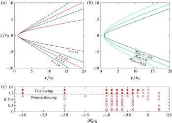
. Following (2.1), the bridge angle can be controlled independently of curvature (figure 7
a). Conversely, curvature can be controlled independently of angle (figure 7
b). The results of a number of simulations show that there exists a critical angle
 ${\it\theta}_{c}$
that has negligible dependence on initial non-dimensional mean curvature
 $\mathscr{H}_{0}r_{0}$
as long as this curvature is sufficiently negative. This dependence is shown in figure 7(c), with filled and open circles corresponding to simulations resulting in coalescence and non-coalescence, respectively. Here the initial mean curvature at the centre of the bridge,
 $\mathscr{H}_{0}$
, is non-dimensionalized by the initial bridge radius
 $r_{0}$
. As expected, positive values of initial non-dimensional mean curvature
 $\mathscr{H}_{0}r_{0}$
result in the immediate collapse of the connecting bridge region, and coalescence is never observed. For a small range of negative values of this curvature,
 ${\it\theta}_{c}$
exhibits a weak dependence on initial geometry. However, with large negative initial mean curvature (
 $\mathscr{H}_{0}r_{0}\gtrsim -0.4$
), the critical transition angle
 ${\it\theta}_{c}$
is negligibly affected.
The effects of initial geometry governed by (2.1) for a variety of initial mean curvatures and cone angles. (a) Cone angle is varied while non-dimensional mean curvature is held constant at
 $\mathscr{H}_{0}r_{0}=-1.0$
. (b) Initial curvature is varied while the cone angle is held at
 ${\it\theta}=1.2$
. (c) Simulations are shown for a range of cone angles and initial mean curvatures. Away from the region where curvature in the bridge is small (
 $\mathscr{H}_{0}r_{0}\approx 0$
) there exists a critical angle
 ${\it\theta}_{c}$
above which all droplets coalesce, and below which all pinch off. There is negligible affect on critical angle by initial mean curvature provided that this mean curvature is sufficiently negative. A dashed line is shown to highlight this critical angle. Filled and unfilled circles represent coalescing and non-coalescing simulations, respectively.

For completeness we also investigated whether the shape of the drop had an appreciable effect on the coalescence dynamics. Indeed, droplets induced to coalesce in electric fields can deform so that they are no longer perfect spheres (figure 1
d). Both prolate and oblate initial droplet geometries are considered. These ellipsoidal droplets are characterized by their semi-major and semi-minor axis
 $a$
and
 $b$
respectively as shown in figure 8(a). The semi-major axis of these elongated droplets is co-linear with the axis of symmetry. The ratio of semi-major to semi-minor axis is
 $a/b=0.5$
and
 $a/b=2.0$
for the prolate and oblate ellipsoids, resulting in eccentricity of
 $e=0.745$
for both topologies. The mean curvature at the scale of
 $R$
at the point closest to the origin for these ellipsoidal droplets is
 $a/b^{2}$
and
 $b/a^{2}$
for prolate and oblate ellipsoids, respectively. The oblate and prolate ellipsoids (figure 8
a) were scaled such that their mean curvature at the point closest to the origin matched the mean curvature,
 $1/R$
, of the spherical droplet. Pairs of these ellipsoids were attached with a hyperboloid following the same procedure as carried out earlier with the spheres (figure 8
a). Cone angles of
 ${\it\theta}=1.2$
and
 ${\it\theta}=1.1$
and initial curvature
 $\mathscr{H}_{0}r_{0}=-1.0$
were investigated and compared with spherical droplets (figure 8
b).
Simulations where the outer droplet geometry has been modified. (a) Prolate and oblate ellipsoidal droplets with eccentricity
 $e=0.745$
are used as initial outer boundary conditions instead of a sphere. The initial mean curvature in the bridge region of both ellipsoids is set to the mean curvature of the spherical droplet
 $1/R$
. (b) The bridge radius
 $\ell (t)$
for a sphere is indistinguishable from either the prolate or oblate ellipsoid at small and intermediate scales despite the large volume differences between all geometries. Only at the largest scales,
 $R$
, are the effects of the different volumes observed.

The results from these simulations are shown in figure 8(b) in the same format as figure 3. The bridge radius
 $\ell (t)$
for the prolate and oblate ellipsoids shows nearly indistinguishable trajectories from the spherical droplets (figure 8
b) at both the early times when initial mean curvature drives the dynamics and at intermediate scales where the cone angle
 ${\it\theta}$
affects coalescence and break-up. Only at the largest scales do the dynamics of the prolate and oblate ellipsoids deviate from that of the spherical droplet. The dynamics of the ellipsoidal droplets with cone angles of
 ${\it\theta}=1.1$
are nearly identical to that of the spherical droplet.
The results illustrate that the outer geometry has a negligible effect on the intermediate asymptotics; significant deviations occur only when the bridge reaches size scales of the droplet.
In our simulations, we observe a regime of self-similar dynamics whenever the conical drops coalesce that appears to be independent of the non-conical geometry. When the drops do not coalesce, the bridge radius
 $\ell$
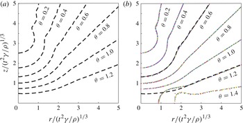
passes through zero as the connected double-cone undergoes a topological rearrangement into two non-connected cones. The dynamics continue beyond this point and the drops continue to recoil (figure 2). The tips of the two conical droplets can each be modelled as a recoiling liquid cone, a geometry that has previously been investigated using the inviscid, self-similar equations (Sierou & Lister Reference Sierou and Lister2004). The results of these previous simulations illustrated that the surface-tension-driven retraction of an inviscid liquid cone would adopt a self-similar profile that depended on the far-field angle,
 ${\it\theta}$
(figure 9
a).
Self-similar profiles for coalescing or recoiling cones at different angles
 ${\it\theta}$
, all with initial mean curvature
 $\mathscr{H}_{0}(c=3)=-1/r_{0}$
. (a) Recoiling profiles of inviscid cones in a vacuum from boundary-integral simulations (Sierou & Lister Reference Sierou and Lister2004) are shown as dashed lines. (b) Dots correspond to the current simulations with overlaid dashed lines again representing the previous boundary-element simulations. As expected, recoiling solutions are nearly indistinguishable (
 ${\it\theta}=0.6$
). Previous simulations of single cones are prescribed to recoil, whereas the current simulations of double-cones can also coalesce (
 ${\it\theta}=1.2$
).

We can similarly plot the recoiling dynamics for the simulations presented here whenever the initially connected drops fail to coalesce. Indeed, the collapsed retracting profiles calculated in this paper (figure 9 b) are nearly indistinguishable from the self-similar inviscid profiles reported by Sierou & Lister (Reference Sierou and Lister2004).
There are two implications of this result. First, the similarity between profiles provides evidence that the computations used in this paper are properly executed and precise enough to capture the essential physics in this problem. Second, the similarity suggests that the results by Sierou & Lister (Reference Sierou and Lister2004) generalize beyond a strictly conical geometry, and are appropriate to model nearly inviscid recoil for conical interfaces as an intermediate asymptotic solution. From a dimensional analysis perspective, the critical angle
 ${\it\theta}_{c}$
can, and most likely does, vary with
 $\mathit{Oh}$
,
 ${\it\rho}_{r}$
and
 ${\it\mu}_{r}$
, all of which have been fixed in this study. However, the similarity in the profiles suggests that when
 $\mathit{Oh}\rightarrow 0$
,
 ${\it\rho}_{r}\rightarrow 0$
and
 ${\it\mu}_{r}\rightarrow 0$
, the critical angle
 ${\it\theta}_{c}$
approaches an asymptotic limit.
When
 ${\it\theta}\geqslant {\it\theta}_{c}$
, the profiles computed by Sierou & Lister (Reference Sierou and Lister2004) no longer match the results from our simulations. This difference is not surprising given that the double-cones are coalescing, as opposed to recoiling, in our simulation. Indeed, if the double-cone is separated into two single cones the result of Sierou & Lister (Reference Sierou and Lister2004) is recovered. Still, the difference does highlight that there are two possible self-similar profiles for a given far-field angle
 ${\it\theta}\geqslant {\it\theta}_{c}$
. The difference also illustrates how the results from this paper are novel, but complementary to the previous literature on inviscid self-similar dynamics of wedges and cones.
4. Conclusions and discussion
The results presented in this paper provide the necessary physical modelling to reconcile differences in existing models of conical drop coalescence and pinch-off. Specifically, the incompressible Navier–Stokes equations were solved to model the coalescence of conical drops under conditions representative of millimetre water drops surrounded by air. The particular conical drop geometries used in this study were motivated by the profiles observed during the initial stage of electrocoalescence. In these observations, two spherical drops deform so that the region near contact appears conical with varying cone angle
 ${\it\theta}$
. We expect that prior to contact, the two conical drops would each have a finite radius of curvature at the tip of the cone. We assume that this curvature would help initiate coalescence upon contact during the microsecond time period that charge effects relax. Thus we have modelled the initial double-cone geometry with three distinct length scales: a small bridge that has a positive mean curvature to initiate coalescence, a conical intermediate scale, and constant curvature away from the bridge region at the largest scale.
As coalescence progresses, the simulations demonstrate that effects of the conical geometry either continue the coalescence or reverse the flow, initiating pinch-off. Our results demonstrate that the dynamics that determine the critical angle between coalescence and recoil is in this intermediate regime, where the bridge can be approximated as two cones. By varying the cone angle between different simulations, we find the drops coalesce when
 ${\it\theta}\geqslant 1.14$
and pinch off and recoil when
 ${\it\theta}\leqslant 1.13$
. Therefore the transition angle is approximately
 $65^{\circ }$
off the axis of rotation, or
 $25^{\circ }$
from the plane normal to the axis of rotation. The latter value is slightly different from the model angle prediction of
 $31^{\circ }$
, but consistent with the experimental transition value of
 $27\pm 2^{\circ }$
(Bird et al.
Reference Bird, Ristenpart, Belmonte and Stone2009).
Previous attempts to model this problem have neglected the influence that fluid inertia has on the neck shape. The results presented here indicate that the neck grows as
 $t^{2/3}$
when
 ${\it\theta}>{\it\theta}_{c}$
, in contrast to previous predictions of
 $t^{1/2}$
(Helmensdorfer Reference Helmensdorfer2012; Helmensdorfer & Topping Reference Helmensdorfer and Topping2013). As a point of reference, it is unlikely that electric fields could produce conical drops with an angle sharper than that of a Taylor cone without other effects such as electrospraying. Therefore it is important to note that the Taylor cone angle of
 ${\it\theta}=49.3^{\circ }=0.86$
(Taylor Reference Taylor1964) is at an angle less than the transition angle, when the cones would already be predicted to recoil. Finally, because our model is independent of any electrical effects, we would expect it to be valid in non-electrical coalescence situations in which nearly inviscid conical drops contact. Facing cone-like protrusions have been observed when drops are pulled apart (Yoon et al.
Reference Yoon, Baldessari, Ceniceros and Leal2007), which can lead to coalescence (Bremond, Thiam & Bibette Reference Bremond, Thiam and Bibette2008). Our results suggest that there may be a similar coalescence–recoil transition for these separating drops.
Acknowledgements
We thank H. A. Stone for helpful comments. We also acknowledge support from the École Polytechnique internship program and Boston University startup funds.