2. The sink-side: palaeogeography and continental silicate weathering

CO₂ consumption by the weathering of silicate rocks exposed at the continental surface depends on air temperature, runoff, lithology, physical erosion and vegetation cover. In the following, we neglect the impact of lithology on the efficiency of weathering. Although the spatial distribution of the outcropping rock types can be estimated for the Cenozoic (Taylor et al. Reference Taylor, Banwart, Valdes, Leake and Beerling2012; Lefebvre et al. Reference Lefebvre, Donnadieu, Goddéris, Fluteau and Hubert-Théou2013), reliable information is lacking for the Mesozoic and Palaeozoic.

2.a. Temperature, runoff and palaeogeography

In deep time carbon cycle models, CO₂ consumption by silicate rock weathering (F _sw) is generally assumed to be linearly dependent on mean annual runoff R and on an Arrhenius-type function of mean annual air temperature T:

(2) $$\begin{equation} {F_{\rm sw}} = k \cdot R \cdot {e^{\left[ {\frac{{ - {E_{\rm a}}}}{\rho } \cdot \left( {\frac{1}{T} - \frac{1}{{{T_0}}}} \right)} \right]}} \end{equation}$$

where ρ is the ideal gas constant, E _a is an apparent activation energy, and T ₀ a reference temperature. k is the weatherability factor. It represents all parameters impacting weathering other than runoff and temperature (Kump & Arthur, Reference Kump, Arthur and Ruddiman1997). At this stage, we keep it constant, which means that physical erosion and land plants impact weathering with the present-day efficiency, whatever the geological period.

The palaeogeography is a critical component in equation (2). Although it does not appear explicitly, palaeogeography exerts a first-order control on the spatial distribution of the temperature and continental runoff, for any given atmospheric CO₂. For instance, a polar location of large continents forces continental temperatures to stay low. Consequently, the efficiency of silicate weathering decreases, forcing CO₂ to rise until the equilibrium described in equation (1) is reached again (Marshall, Walker & Kuhn, Reference Marshall, Walker and Kuhn1988). Similarly, the presence of a supercontinent inhibits the runoff in the large and dry continental interiors, forcing CO₂ to rise (Gibbs et al. Reference Gibbs, Bluth, Fawcett and Kump1999; Goddéris et al. Reference Goddéris, Donnadieu, Le Hir, Lefebvre and Nardin2014).

Incorporating the role of palaeogeography in the geological carbon cycle requires spatially resolved models. The GEOCLIM model (Donnadieu et al. Reference Donnadieu, Goddéris, Pierrehumbert, Dromart, Jacob and Fluteau2006; Goddéris et al. Reference Goddéris, Donnadieu, Le Hir, Lefebvre and Nardin2014) couples a three-dimensional climate model with a box-model describing the global carbon cycle. GEOCLIM operates as follows: starting from an initial arbitrary state of the carbon cycle and the corresponding atmospheric CO₂, the climate module of GEOCLIM calculates the mean annual continental temperatures and runoff with a spatial resolution of 7.5° long × 4.5° lat. Continental runoff is equal to the difference between atmospheric precipitation and evapotranspiration for each continental grid cell. The temperature and runoff fields are then used to calculate the CO₂ consumption by silicate weathering on each continental grid cell using equation (2). The corresponding total silicate weathering is sent to the geochemical model, which calculates a new atmospheric CO₂ pressure. The updated CO₂ is sent back to the climate model to update temperature and runoff fields. This procedure is repeated until the steady state described by equation (1) is reached.

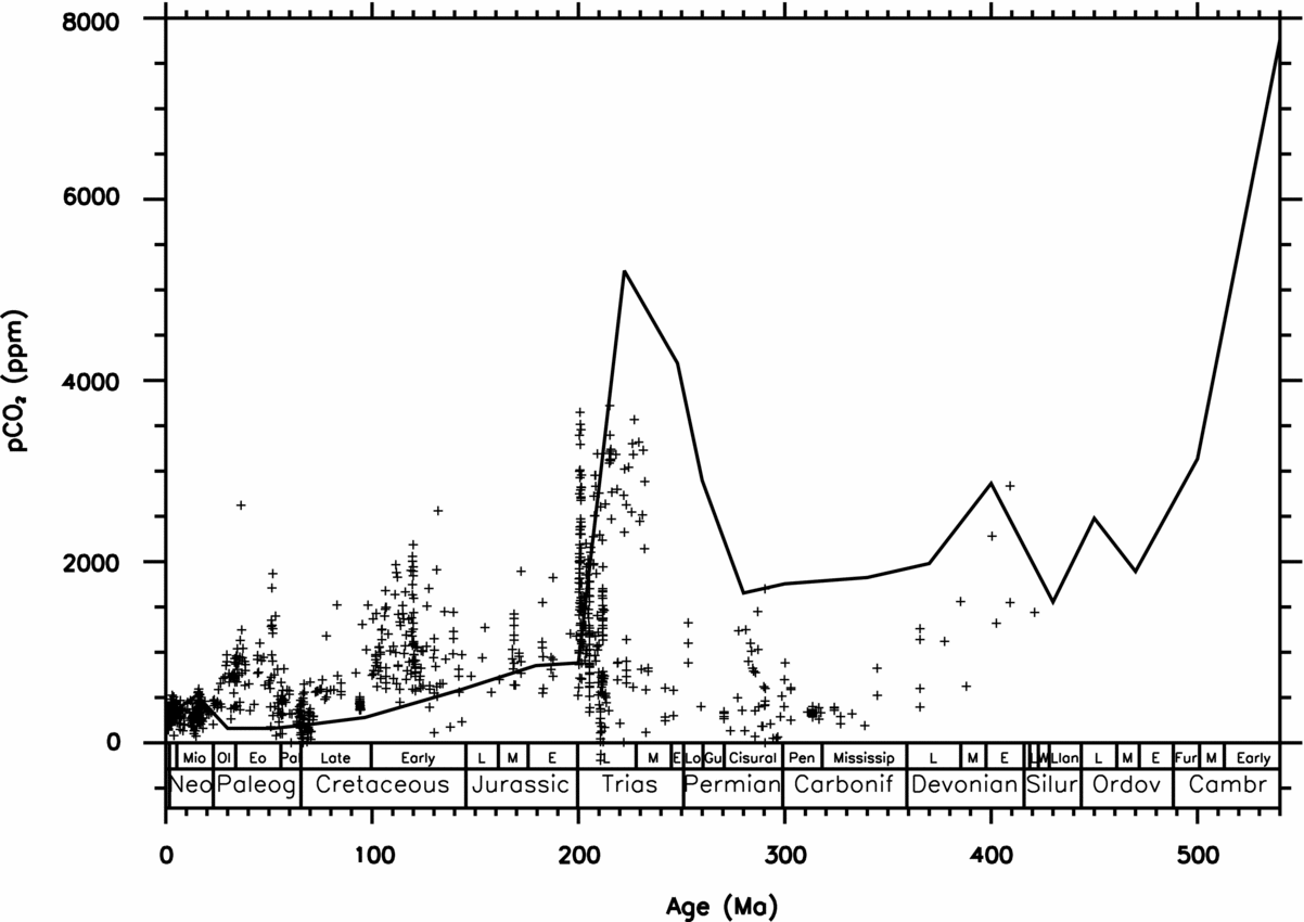
Following this procedure, we calculate atmospheric CO₂ levels for 22 time slices covering the whole Phanerozoic (see Section 1 and Goddéris et al. Reference Goddéris, Donnadieu, Le Hir, Lefebvre and Nardin2014). The solar constant is assumed to rise linearly from the past towards the present day. The solid Earth degassing is held constant, so that the role of palaeogeography in modulating weathering rates and CO₂ is emphasized (Fig. 1). This simulation is referred as GEOCLIMtec in the following.

Figure 1.

Calculated evolution of the atmospheric CO₂ concentration (GEOCLIMtec simulation). The CO₂ flux released by magmatism is held constant at its present-day value. Crosses represent the data (Royer, Reference Royer, Holland and Turekian2014).

Those simulations have been extensively discussed in Goddéris et al. (Reference Goddéris, Donnadieu, Le Hir, Lefebvre and Nardin2014), and here we briefly summarize the key results. Since the amount of energy received from the sun rises from the Cambrian to the present day, the amount of CO₂ required to balance the CO₂ consumed by silicate weathering and the constant degassing decreases with time. One of the main features of the calculated CO₂ is the existence of high CO₂ levels within the 280–220 Ma time window (Fig. 1). These correspond to the period of existence of the Pangaea supercontinent, where the climate model predicts dry conditions above large continental surfaces, which inhibit weathering, pushing CO₂ levels to rise (Donnadieu et al. Reference Donnadieu, Goddéris, Pierrehumbert, Dromart, Jacob and Fluteau2006). Another striking feature is the decline of the calculated CO₂ level from 540 Ma to the end Ordovician and early Silurian. This trend is related to a progressive rise in temperature and runoff over Laurentia, Baltica and Siberia as these three continents move across the equator (Nardin et al. Reference Nardin, Goddéris, Donnadieu, Le Hir, Blakey, Pucéat and Aretz2011). As a result, CO₂ decreases and the global climate cools so that the balance between global silicate weathering and constant solid Earth degassing is still achieved. Another striking feature is the constancy of the palaeogeographic signal over the period extending from 180 to 0 Ma. The signal is flat, and suggests that the dispersed continental configuration over a wide range of latitudes promotes low levels of CO₂ since the Jurassic. Lastly, the Permo-Carboniferous glaciation cannot be explained by the palaeogeographic modulation of weathering. The palaeogeographic forcing does not generate a clear drop in the atmospheric CO₂ at the time of the glaciation.

2.b. Robustness of the palaeogeographic imprint on the atmospheric CO₂ evolution

The calculated impact of the palaeogeography on the atmospheric CO₂ evolution depends on the impact of the climate on the silicate weathering. The weathering law used to simulate the CO₂ consumption is thus critical. Equation (2) predicts the maximum silicate weathering in the equatorial region where runoff and temperature are optimal. However, the development of thick weathering profiles in those zones shifts the weathering system from a kinetically limited mode to a transport-limited mode. As a result, despite high runoff values, flat equatorial areas are mostly characterized by low weathering rates (Gaillardet et al. Reference Gaillardet, Dupré, Louvat and Allègre1999). Equation (2) may introduce a potentially important bias by overestimating the weight of the equatorial area in the global weathering budget. Such an overestimate may promote too low CO₂ and too cold climate when the fraction of continental surface located in the climatic convergence belt increases.

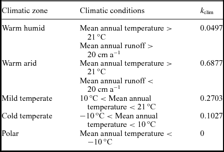
As a simple test, we replaced equation (2) by a set of four equations stating that CO₂ consumption by continental silicate weathering for each continental grid cell is proportional to the local runoff (‘geoderma’ run). The proportionality constant depends on the climatic zone where the grid cell is located. Four climatic zones have been defined: warm and humid, warm and arid, mild temperate, and cold temperate, following the methodology proposed by Goddéris et al. (Reference Goddéris, Donnadieu, Tombozafy and Dessert2008). Each of these proportionality constants has been calibrated using the Gaillardet et al. (Reference Gaillardet, Dupré, Louvat and Allègre1999) global riverine database. Equation (2), which is defined on each continental grid cell, is thus replaced by the following equation, also applied on each continental grid cell:

(3) $$\begin{equation} {F_{\rm sw}} = {k_{\rm clim}} \cdot R \end{equation}$$

where F _sw is the CO₂ consumption by silicate weathering for a given continental grid element and R the mean annual runoff for this grid cell. k _clim is a proportionality factor which depends on the climatic conditions prevailing for the considered cell (Table 1). This weathering law (equation 3) does not account explicitly for the topography of the continents. Consequently, there is potentially a risk that the weathering flux from equatorial mountain ranges is underestimated, because of the assignment of a very low value to k _clim. However, the climatic fields (temperature and runoff) have been calculated with the presence of reliefs on the continents. The calculated temperature drops in mountainous areas and the corresponding grid cells fall in the mid-temperate weathering zone. As a corollary, the warm and humid climatic zones defined by the model always correspond to flat area.

Table 1.

Proportionality constants linking CO₂ consumption by silicate weathering to the mean annual runoff for each grid cell, as a function of the climatic zone to which the cell belongs (Goddéris et al. Reference Goddéris, Donnadieu, Tombozafy and Dessert2008).

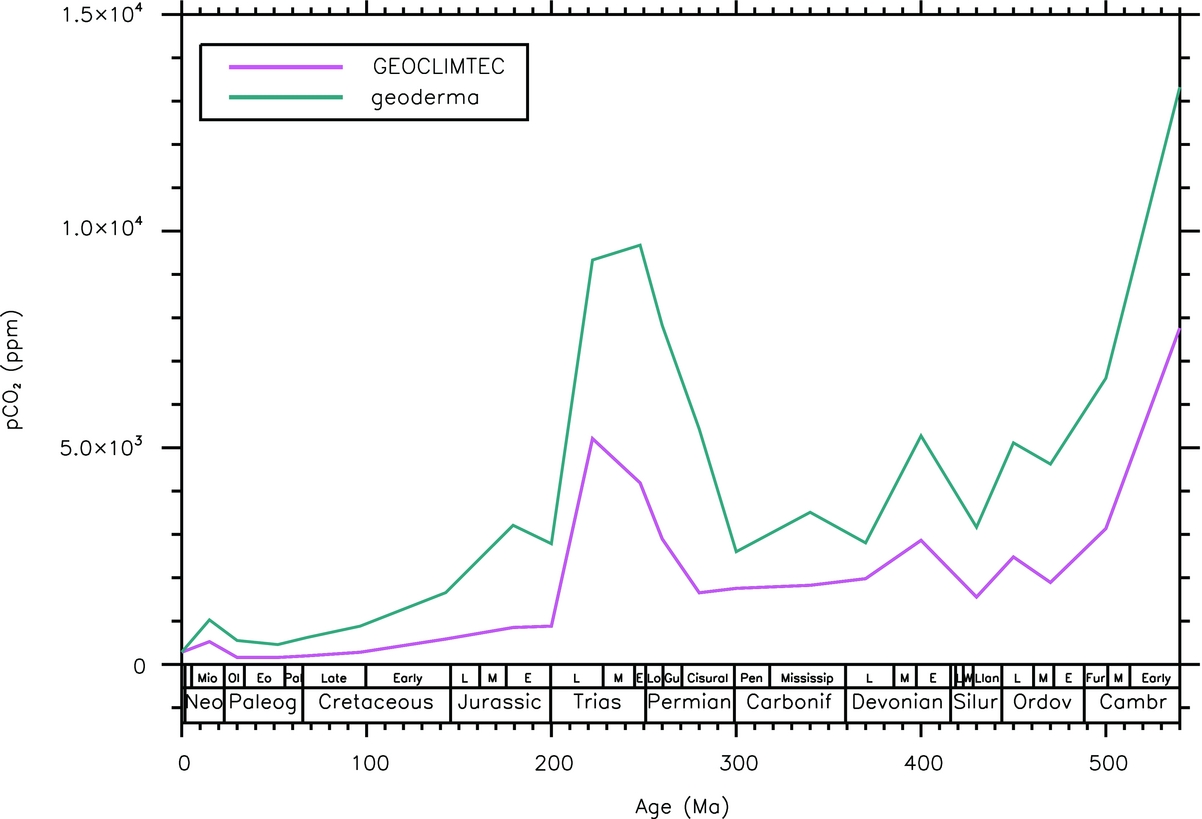
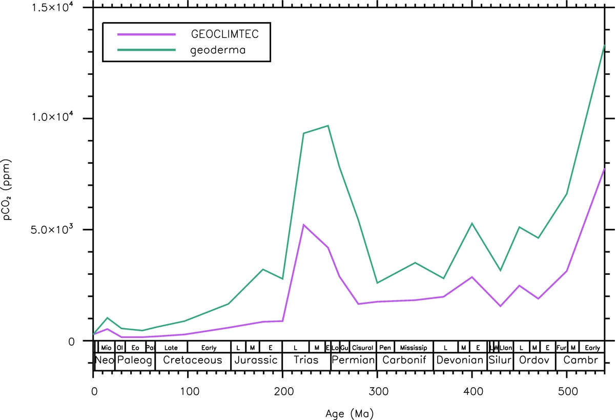
In response, the GEOCLIM model significantly decreases the weathering flux originating from the equatorial area, and reinforces the contribution from the middle latitudes for each of the simulated Phanerozoic time slices. Despite this important reorganisation in the spatial pattern of the weathering flux, the overall trend remains quite unchanged (Fig. 2, geoderma simulation). The major features remain remarkably stable. The early Phanerozoic CO₂ decrease, the Permo-Triassic peak and the CO₂ flattening since the middle Mesozoic are still predicted.

Figure 2.

Calculated Phanerozoic evolution of the atmospheric CO₂ in the reference GEOCLIMtec run, and assuming the existence of a soil shielding effect (GEODERMA simulation).

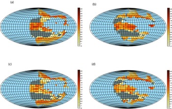
It is somewhat surprising that the CO₂ evolution is so weakly sensitive to the mathematical representation of the weathering flux. We further explore the behaviour of the carbon cycle between 220 and 200 Ma (Fig. 3). These two time slices have been chosen because the continental drift is responsible for a huge drop in CO₂ in the standard GEOCLIMtec run (using equation 2), which is also predicted in the ‘geoderma’ run. For both ages, the ‘geoderma’ simulation predicts a spatial redistribution and a global lowering of the weatherability of the continents compared to the standard runs of the same age. But in both sets of simulations, the overall increase of the continental global runoff, related to the northward drift of Pangaea, forces CO₂ to decrease. Indeed, the continental surface located in the humid convergence zone increases from 220 to 200 Ma (Goddéris et al. Reference Goddéris, Donnadieu, Le Hir, Lefebvre and Nardin2014). In the standard GEOCLIMtec simulation, this increase allows the development of extremely efficient weathering along the equator. In the ‘geoderma’ run, the implicit development of thick regoliths limits the increase in equatorial weathering. But the rise in equatorial runoff is strong enough to generate two weathering hotspots at the equator (above Northwest Africa and South China) at 200 Ma, responsible for the CO₂ drawdown (Fig. 3).

Figure 3.

Calculated shield rock weathering (log10 of the associated atmospheric CO₂ consumption in Gmol a⁻¹) for two time slices, from two sets of simulations. Each map is displayed at steady-state atmospheric CO₂, assuming a fixed magmatic CO₂ degassing. (a) 220 Ma – GEOCLIMtec – atmospheric CO₂ = 5200 ppm; (b) 200 Ma – GEOCLIMtec – atmospheric CO₂ = 880 ppm; (c) 220 Ma – GEODERMA simulation accounting for the shielding effect of thick saproliths – atmospheric CO₂ = 9300 ppm; (d) same as (c) but at 200 Ma, atmospheric CO₂ = 2800 ppm.

In both simulations, the control exerted by the continental configuration on the runoff is responsible for first-order changes in atmospheric CO₂. This is not surprising in the standard case, where silicate weathering depends linearly on runoff. But this result is not obvious for the ‘geoderma’ simulation, where dependence of the proportionality constant on the climatic zone introduces a non-linearity in the response of continental weathering to runoff.

3. The source-side: Earth CO₂ degassing and atmospheric CO₂ evolution

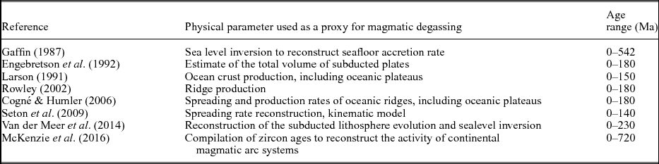
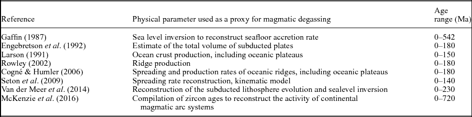
There is no direct and unique proxy for reconstructing the past CO₂ degassing by magmatic activity. Various proxies can be used to infer past degassing (Table 2): inversion of the sea level fluctuations to calculate past volume of the mid-oceanic ridges (Gaffin, Reference Gaffin1987), reconstruction of the seafloor production rate at mid-oceanic ridges (Larson, Reference Larson1991; Rowley, Reference Rowley2002; Cogné & Humler, Reference Cogné and Humler2006; Seton et al. Reference Seton, Gaina, Müller and Heine2009), reconstruction of subducted volumes (Engebretson et al. Reference Engebretson, Kelley, Cashman and Richards1992; Rowley, Reference Rowley2002; Hoareau et al. Reference Hoareau, Bomou, van Hinsbergen, Carry, Marquer, Donnadieu, Le Hir, Vrielynck and Walter-Simonnet2015), compilation of zircon age (McKenzie et al. Reference McKenzie, Horton, Loomis, Stockli, Planavsky and Lee2016), and reconstruction of the subduction zone length as a function of age (Van der Meer et al. Reference Van der Meer, Zeebe, van Hinsbergen, Sluijs, Spakman and Torsvik2014). Most of these reconstructions focus on the last 200 Ma because older geological materials have been subducted. Two reconstructions extend over the whole Phanerozoic (Gaffin, Reference Gaffin1987; McKenzie et al. Reference McKenzie, Horton, Loomis, Stockli, Planavsky and Lee2016). Translating these proxies into moles of carbon released into the atmosphere is not an easy task. These indices are not equivalent: some of them trace the evolution of arc volcanism through time (McKenzie et al. Reference McKenzie, Horton, Loomis, Stockli, Planavsky and Lee2016), while others estimate the volume of mid-oceanic ridges (Gaffin, Reference Gaffin1987). Generally, modellers assume a simple proportionality between the geological indices and the global CO₂ degassing rate. This is a critical assumption, but the various components of the total flux (at least arc volcanism and degassing at mid-oceanic ridges) are heavily dependent on the oceanic spreading rate, and some proportionality between them might reasonably be expected.

Table 2.

Proxies used to constrain the magmatic degassing of the Earth.

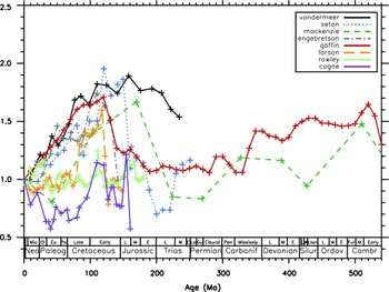
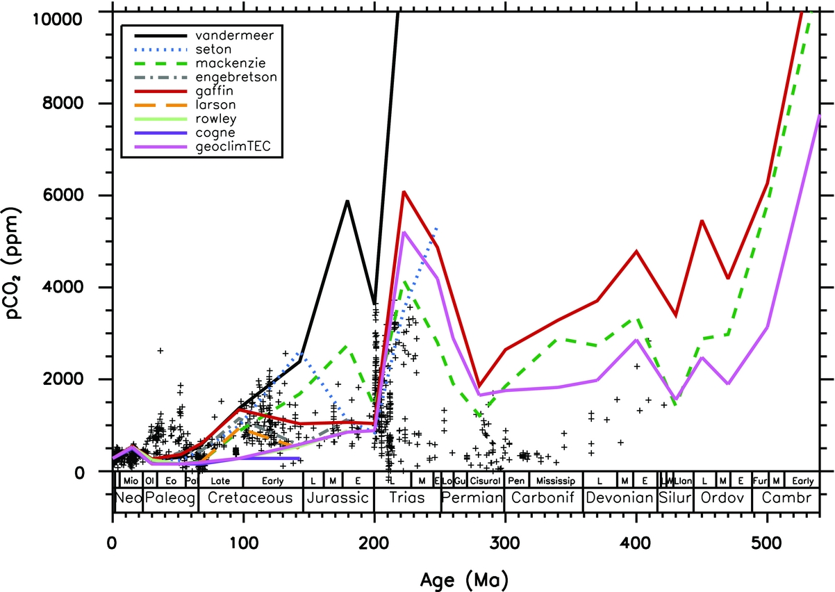
Owing to the method and to the degassing index used, the reconstructed histories of the degassing rate display different patterns (Fig. 4). For instance, the CO₂ degassing rate at 100 Ma might be similar to the present-day degassing, or might be enhanced by 100 %.

Figure 4.

Indices for the evolution of the solid Earth degassing rate (normalized to the indices for the evolution of the solid Earth degassing rate (normalized to their present-day values)). See Table 2 for references.

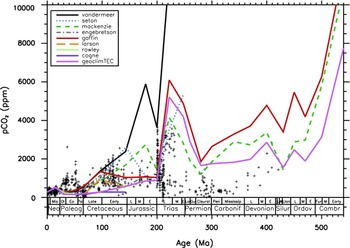
Numerical models of the geological carbon cycle are sensitive to the degassing rate. We forced the GEOCLIM model with all the degassing indices listed in Table 2, and kept the palaeogeographic forcing active (Fig. 5). Going from the present to the past, most of the degassing scenarios induce an increase in the CO₂ level in the Early Cenozoic, counteracting the palaeogeographic forcing which was driving CO₂ to too low values (Lefebvre et al. Reference Lefebvre, Donnadieu, Goddéris, Fluteau and Hubert-Théou2013). The calculated CO₂ levels for each degassing index then rapidly diverge when looking further back in time. Most of the simulations suggest a higher CO₂ in the Cretaceous compared to the simulation at constant degassing rate. Around the Turonian climatic optimum (90 Ma), the original GEOCLIMtec simulation was predicting only 300 ppm of CO₂. Accounting for a variable degassing, the atmospheric CO₂ now ranges from 300 to 1500 ppmv, depending on the proxy used (Fig. 5). Several reconstructions (Gaffin, Reference Gaffin1987; Larson, Reference Larson1991; Engebretson et al. Reference Engebretson, Kelley, Cashman and Richards1992) predict a peak in CO₂ around 100 Ma, but the other reconstructions predict a continuous rise going back in time into the Jurassic. The degassing scenarios reinforce the CO₂ rise linked to the final assembly of Pangaea, except one (McKenzie et al. Reference McKenzie, Horton, Loomis, Stockli, Planavsky and Lee2016). Regarding the Palaeozoic, only two reconstructions are available (Gaffin, Reference Gaffin1987; McKenzie et al. Reference McKenzie, Horton, Loomis, Stockli, Planavsky and Lee2016). Once injected into the GEOCLIM model, they all predict very high CO₂ in the early Palaeozoic, close to 10 000 ppmv. Using a variable degassing improves the Carboniferous CO₂ history slightly, by predicting an overall CO₂ decrease, qualitatively consistent with the onset of the Late Palaeozoic ice age.

Figure 5.

Calculated evolution of the atmospheric CO₂ concentration (GEOCLIMtec simulation). The CO₂ flux released by magmatism is constrained by the various proxies described in Table 2. Crosses represent the data (Royer, Reference Royer, Holland and Turekian2014).

4. Palaeogeography or CO₂ degassing: which is the main driver?

The simulations performed with a variable CO₂ degassing rate include the palaeogeographic forcing as well as the effect of the rising solar constant with time. Deciphering the relative importance of these processes requires isolating each of them. We start with the CO₂ evolution calculated by the GEOCLIMtec simulations, in which magmatic degassing is held constant through time. First, we remove the effect of the increasing solar luminosity (Gough, Reference Gough1981) by subtracting a linear fit of the model output (minimizing chi-square fit), so that the palaeogeographic forcing remains the only forcing of the carbon cycle. Then, to illustrate the role of the degassing rate on the CO₂ history, we run two additional sets of simulations. In the first set, we assume that the palaeogeography of each stage of the Phanerozoic is the 30 Ma configuration, and we calculate the atmospheric CO₂ over the whole Phanerozoic, assuming a variable degassing. We repeat this procedure keeping the palaeogeography fixed at the 220 Ma configuration. This method allows us to subtract the impact of palaeogeography and to ‘freeze’ the solar constant. The 30 Ma palaeogeography was chosen as the continental configuration producing the higher silicate weathering flux at any given CO₂ concentration compared to other time slices. The continental configuration at 30 Ma maximizes the silicate rock weatherability. Conversely, the 220 Ma palaeogeography is the driest configuration, corresponding to the weakest weatherability.

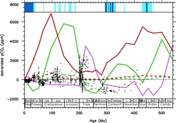
This procedure generates several CO₂ curves, which can be interpreted as the strength of the various forcings (Fig. 6). Maximum values mean that the corresponding forcing (palaeogeography or degassing) is driving the system into a warm mode characterized by high CO₂ levels. Conversely, minimum values correspond to a cold mode forcing. From Figure 6, it is clear that the continental configuration regulates the amplitude of the CO₂ response to a change in degassing. A dispersed configuration, such as the Oligocene one (30 Ma), buffers the impact of a variable degassing on atmospheric CO₂. Conversely, weathering flux in a supercontinental configuration exerts a weak control on the CO₂ fluctuations induced by a variable degassing. A second striking feature in Figure 6 is the apparent anticorrelation between the palaeogeographic forcing and the degassing forcing of the atmospheric CO₂ changes. In the lower Palaeozoic, the palaeogeographic setting forces CO₂ to reach a minimum value around the late Ordovician – early Silurian, while the degassing function reaches its maximum at the same time (at least when the Gaffin index is used. The Mc- Kenzie forcing reaches its coldest mode at the end of the Llandovery, just after the glacial event). Then both indices of the degassing impact on the CO₂ evolution reach their minimum values around the end Permian/ early Triassic, while the palaeogeography generates the hottest conditions of the Phanerozoic. Conversely, the palaeogeographic forcing generates a cold forcing in the last 200 Ma of Earth history, while degassing indices generate warm climatic conditions, particularly in the Late Cretaceous and Early Cenozoic.

Figure 6.

Detrended Phanerozoic CO₂ evolution. The pink curve is the GEOCLIM model output when the changing palaeogeography is the only forcing. The curve has been detrended in an attempt to capture the effect of the decreasing solar constant through time. The two green curves represent the CO₂ trends when the only forcing is the degassing rate indexed on the McKenzie et al. data. The two red curves show the CO₂ trends when the degassing is indexed on the inversion of the Phanerozoic sealevel from Gaffin. The dashed and solid lines are the simulations where the palaeogeography is held constant at 30 Ma or 220 Ma respectively. The present-day CO₂ values have been subtracted in each of these four simulations. Data (crosses) are from Royer and have been detrended as well. Vertical blue bars at the top represent cold (light blue) and glacial (deep blue) episodes (Dera et al. Reference Dera, Brigaud, Monna, Laffont, Pucéat, Deconinck, Pellenard, Joachimski and Durlet2011; Nardin et al. Reference Nardin, Goddéris, Donnadieu, Le Hir, Blakey, Pucéat and Aretz2011; Friedrich, Norris & Erbacher, Reference Friedrich, Norris and Erbacher2012; Montanez & Poulsen, Reference Montanez and Poulsen2013; Bodin et al. Reference Bodin, Meissner, Jansen, Steuber and Mutterlose2015; Montanez, Reference Montanez2016)

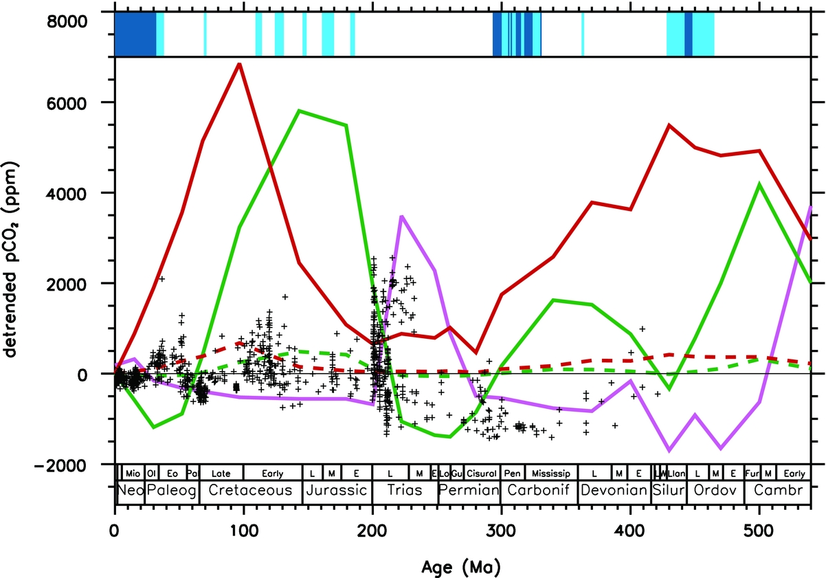
These results strongly suggest that the CO₂ fluctuations over the last 200 Ma cannot be explained by the palaeogeographic configuration, and require a variable magmatic degassing rate. Conversely, the palaeogeographic configuration is the key driver of the CO₂ evolution from the Cambrian to the Jurassic. This general framework suffers from one noticeable exception. Neither the continental horizontal drift nor the reconstructed degassing can satisfactorily explain the onset of the Late Palaeozoic ice age. This cold episode is often related to the colonization of the continental surfaces by vascular plants, which may have promoted CO₂ consumption by silicate weathering and organic carbon burial (Berner, Reference Berner2004). A recent study challenges this hypothesis, and emphasizes the role of vertical tectonics (uplift of the Hercynian mountains) on the physical erosion and chemical weathering (Goddéris et al. Reference Goddéris, Donnadieu, Carretier, Aretz, Dera, Macouin and Regard2017).

5. Cold and warm climate modes of the Phanerozoic

In the above discussion, we focused on the time evolution of the atmospheric CO₂. Can we draw similar conclusions regarding the Earth surface temperature? Geological cold climatic episodes generally correspond to periods characterized by the existence of perennial ice at low altitude on the continents. For this reason, we think that it is more pertinent to plot the continental surface below a mean annual temperature of 0 °C, instead of discussing the time evolution of the averaged global or continental temperatures. However, we must keep in mind that a mean annual temperature below 0 °C does not necessarily imply the existence of perennial ice. It is beyond the objectives and capacities of this study to calculate the continental ice volumes for each scenario tested here. The following discussion must be considered as a basis for future work.

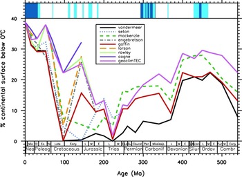
The GEOCLIMtec simulation, performed assuming a constant magmatic degassing, predicts that the continental surfaces being annually below 0 °C fluctuates from a maximum of 40 % of the total continental surface at the present day to 0 % of the continents in the Late Triassic (Fig. 7). When accounting for a variable degassing, the climatic output is not improved for the Palaeozoic and early Mesozoic. The variable degassing scenarios all predict a lower continental surface below the freezing point than the GEOCLIMtec run for the period spanning the Late Palaeozoic ice age.

Figure 7.

Calculated percentage of the total continental surfaces with mean annual temperature below 0 °C, as a function of time. GEOCLIMtec is the simulation with a constant magmatic CO₂ degassing, and accounting for the continental drift. The other curves have been calculated accounting for the evolving palaeogeography and for a variable degassing from various sources. Vertical blue bars at the top represent cold (light blue) and glacial (deep blue) episodes (Dera et al. Reference Dera, Brigaud, Monna, Laffont, Pucéat, Deconinck, Pellenard, Joachimski and Durlet2011; Nardin et al. Reference Nardin, Goddéris, Donnadieu, Le Hir, Blakey, Pucéat and Aretz2011; Friedrich, Norris & Erbacher, Reference Friedrich, Norris and Erbacher2012; Montanez & Poulsen, Reference Montanez and Poulsen2013; Bodin et al. Reference Bodin, Meissner, Jansen, Steuber and Mutterlose2015; Montanez, Reference Montanez2016).

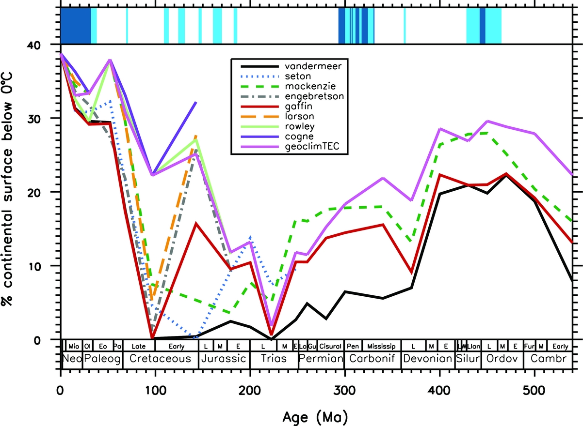
The most striking improvement of the variable degassing simulations compared to the GEOCLIMtec run is the warming of the Earth surface around the Early to Late Cretaceous boundary.