





1. Introduction
Vortex rings have long held a special place in the hearts and minds of many researchers due to their seemingly simple and elegant toroidal structures. This has prompted many experimental, numerical and theoretical studies over the past few decades to unravel their fundamental characteristics and behaviour. These pursuits were also motivated by their frequent occurrences in nature, appearing in various sizes and forms, from smoke rings and volcanic eruptions (Taddeucci et al. Reference Taddeucci, Peña Fernández, Cigala, Kueppers, Scarlato, Del Bello, Ricci, Sesterhenn and Panunzi2021), cardiovascular systems (Martínez-Legazpi et al. Reference Martínez-Legazpi2014), jellyfish motions (Gemmell et al. Reference Gemmell, Troolin, Costello, Colin and Satterlie2015), dandelion flight (Cummins et al. Reference Cummins, Seale, Macente, Certini, Mastropaolo, Viola and Nakayama2018) and industrial applications such as mass production of shaped particles (An et al. Reference An, Warning, Yancey, Chang, Kern, Datta, Steen, Luo and Ma2016). It should not come as a surprise then that much has been learnt about vortex rings, especially when it comes to circular vortex rings (CVRs), where their axisymmetric configuration represents the simplest form of vortex rings possible. For instance, much effort has been expended in the study of their formations, evolutions, formation times, instabilities, mixing and entrainment levels, among other characteristics (Maxworthy Reference Maxworthy1972, Reference Maxworthy1974; Widnall, Bliss & Tsai Reference Widnall, Bliss and Tsai1974; Saffman Reference Saffman1978; Friedman & Turkington Reference Friedman and Turkington1981; Glezer Reference Glezer1988; Shariff & Leonard Reference Shariff and Leonard1992; Nitsche & Krasny Reference Nitsche and Krasny1994; Lim & Nickels Reference Lim and Nickels1995; James & Madnia Reference James and Madnia1996; Heeg & Riley Reference Heeg and Riley1997; Gharib, Rambod & Shariff Reference Gharib, Rambod and Shariff1998; Mohseni & Gharib Reference Mohseni and Gharib1998; Shusser & Gharib Reference Shusser and Gharib2000; Mohseni, Ran & Colonius Reference Mohseni, Ran and Colonius2001; Allen & Auvity Reference Allen and Auvity2002; Dabiri & Gharib Reference Dabiri and Gharib2004; Krueger, Dabiri & Gharib Reference Krueger, Dabiri and Gharib2006; Olcay & Krueger Reference Olcay and Krueger2008; Sullivan et al. Reference Sullivan, Niemela, Hershberger, Bolster and Donnelly2008; Cheng, Lou & Lim Reference Cheng, Lou and Lim2010; Gao & Yu Reference Gao and Yu2010; Stewart et al. Reference Stewart, Niebel, Jung and Vlachos2012; Kleckner & Irvine Reference Kleckner and Irvine2013; Danaila, Kaplanski & Sazhin Reference Danaila, Kaplanski and Sazhin2015; Das, Bansal & Manghnani Reference Das, Bansal and Manghnani2017; Hattori, Blanco-Rodríguez & Le Dizès Reference Hattori, Blanco-Rodríguez and Le Dizès2019; Limbourg & Nedić Reference Limbourg and Nedić2021; Matsuzawa et al. Reference Matsuzawa, Mitchell, Perrard and Irvine2023; Liu & Xu Reference Liu and Xu2025). Note that these understandings further motivate studies on synthetic jets where they essentially comprise vortex-ring trains (Glezer & Amitay Reference Glezer and Amitay2002; Shuster & Smith Reference Shuster and Smith2007; Hong, Cheng & Zhong Reference Hong, Cheng and Zhong2020; Xu & Wang Reference Xu and Wang2024), as well as their mutual interactions or with solid boundaries (Walker et al. Reference Walker, Smith, Cerra and Doligalski1987; Lim & Nickels Reference Lim and Nickels1992; Orlandi & Verzicco Reference Orlandi and Verzicco1993; Mansfield, Knio & Meneveau Reference Mansfield, Knio and Meneveau1999; Couch & Krueger Reference Couch and Krueger2011; Xu & Wang Reference Xu and Wang2016), just to name a few among many other considerations.
Other than CVRs, the second most investigated type of vortex rings will probably be elliptic vortex rings (EVRs). Elliptic vortex rings retain the basic continuous and curved structure, with the distinctive exception of possessing non-uniform circumferential diameters. Their non-uniform curvatures typically lead to circumferential variations in the momentum thickness, induced velocities, as well as mixing and entrainment behaviour, among others. In particular, EVRs demonstrate axis-switching behaviour which is not present in CVRs and continues to be one of the key flow mechanisms not only as isolated vortex ring but also in freely exhausting elliptic jets. These can be readily discerned in some of the more fundamental studies on EVRs and elliptic jets conducted earlier (Dhanak & Bernardinis Reference Dhanak and Bernardinis1981; Ho & Gutmark Reference Ho and Gutmark1987; Oshima et al. Reference Oshima, Izutsu, Oshima and Hussain1988; Hussain & Husain Reference Hussain and Husain1989; Kiya et al. Reference Kiya, Toyoda, Ishii, Kitamura and Ohe1992; Kinzie & McLaughlin Reference Kinzie and McLaughlin1999; Yoon & Lee Reference Yoon and Lee2003; Quinn Reference Quinn2007; Kaplanski, Fukumoto & Rudi Reference Kaplanski, Fukumoto and Rudi2012; Chen et al. Reference Chen, Wang, Li and Wang2016; Cheng et al. Reference Cheng, Lou and Lim2016, Reference Cheng, Lou and Lim2019; Shi, Feng & Wang Reference Shi, Feng and Wang2019; Li & Hong Reference Li and Hong2024; Li & Zhang Reference Li and Zhang2026), where their implementations under impingement conditions lead to favourable heat transfer and mixing characteristics (Lee et al. Reference Lee, Lee and Lee1994; Lee & Lee Reference Lee and Lee2000; Bhapkar, Srivastava & Agrawal Reference Bhapkar, Srivastava and Agrawal2014; Xu & New Reference Xu and New2025b
; Wen, Wang & Xu Reference Wen, Wang and Xu2025). One of the most important working parameters dictating EVR behaviour will be the aspect ratio (
 $ \textrm{AR}$
) of the elliptic orifice/nozzle that produces it, defined as the ratio of the major diameter to the minor diameter. It is known that if it exceeds a threshold value of approximately
 $ \textrm{AR}=4$
, the EVR will not undergo regular axis-switching behaviour. Instead, it will undergo a unique vortex disconnection and reconnection process where the EVR filament segments along the major axis would come into contact and interact with each other. This is due to significant induced velocities caused by the very small radii of curvature that these EVR filament segments possess, which would subsequently lead to the formation of a ‘bridge’ and bifurcation of such an EVR.
On the other hand, much less well-studied basic vortex-ring types will include square or rectangular vortex rings (SVRs and RVRs). Unlike EVRs which possess smooth circumferential variations in terms of their outlines, SVRs/RVRs are produced by orifices or nozzles with four straight sides and four sharp discontinuous corners. In fact, a square geometry can be treated as an
 $ \textrm{AR}=1$
rectangular geometry. Each sharp corner leads to a vortex-ring segment that has a very small radius of curvature, which in turn produces much higher induced velocities relative to the straight segments. Other than that, RVRs are also primarily characterised by their ARs, much like EVRs. Earlier studies on SVRs/RVRs typically arose from the investigations of starting, continuous or synthetic rectangular jets, on top of discrete RVR structures (Grinstein Reference Grinstein2001; Ai et al. Reference Ai, Yu, Law and Chua2005; Wang et al. Reference Wang, Feng, Wang and Li2018; Ghasemi et al. Reference Ghasemi, Tuna and Li2018, Reference Ghasemi, Tuna and Li2019; Lindstrom & Amitay Reference Lindstrom and Amitay2019; Straccia & Farnsworth Reference Straccia and Farnsworth2020; Kumar et al. Reference Kumar, Saha, Panigrahi and Karn2021; Zheng, Gao & Yu Reference Zheng, Gao and Yu2023; Yanaoka & Hatakeyama Reference Yanaoka and Hatakeyama2023). Interestingly, nearly all studies relied on relatively idealised initial conditions to generate isolated RVRs or to look at RVRs as part of starting jets, synthetic or continuous jet flows. While much understanding has been gained so far, it should be highlighted that, in practical experiments involving isolated vortex rings, impulsively piston-driven ‘cylindrical-slug’-based vortex-ring generations are almost always used, and it will be no different for RVRs. However, few, if any, experimental or numerical studies made efforts to make use of such an approach. From a fundamental flow dynamics point of view, while generating RVRs through more idealised initialisations made things more straightforward, there exist several real-world nuances that idealised initialisations could not capture.
First, any over-pressure effects (Didden Reference Didden1979) associated with RVRs generated by an impulsively driven piston would not have been incorporated. These over-pressure effects would ultimately lead to time-dependent exit velocity profiles that vary continuously and impact upon the RVR formation and circulation levels. This is in contrast to a RVR produced using a prescribed, time-invariant velocity profile as assumed by the slug model. As shown by earlier studies (Krueger & Gharib Reference Krueger and Gharib2003; Krueger Reference Krueger2005), over-pressure effects are linked to increased entrained fluid during the impulsively driven stage and the conventional slug model needs to be corrected to account for the higher circulations observed in vortex rings generated impulsively. Such a correction would then lead to better impulse and thrust predictions over the conventional ‘cylindrical-slug’ model, and more optimised outcomes for starting-jet-based propulsion strategies. Second, more idealised RVR initialisations would not be able to take into account the effects of stopping vortex rings produced in experiments when the piston comes to an abrupt stop (Cater, Soria & Lim Reference Cater, Soria and Lim2004; Syed & Sung Reference Syed and Sung2009; Das et al. Reference Das, Bansal and Manghnani2017). Unlike CVRs where one could allow them to translate sufficiently far away from the nozzle/orifice in attempts to minimise the effects of such stopping vortex rings, it is very challenging to do the same for RVRs since they undergo vortical changes due to their axis-switching behaviour shortly after they are formed. Due to the above considerations, the overall circulation, vortex-core trajectory and other key characteristics for a RVR generated by an impulsively driven piston are expected to differ from those predicted by numerical simulations based on more idealised initialisation conditions. Despite this, however, few concrete and systematic efforts to address this systematically can be found.
With the preceding concerns in mind, the present study seeks to shed more light on several key questions. First, while over-pressure effects are well documented and understood for CVRs produced by impulsively driven pistons where over-pressure corrections have been proposed (Krueger Reference Krueger2005; Krieg & Mohseni Reference Krieg and Mohseni2013; Schlueter-Kuck & Dabiri Reference Schlueter-Kuck and Dabiri2016), this is not the case for RVRs produced using the same approach. Hence, one of the questions will be, how will the over-pressure phenomenon for the present flow scenario compares with that for CVRs, especially with regards to how the exit velocity profiles vary temporally along the major and minor planes of a rectangular orifice/nozzle? Earlier experimental and numerical studies on RVRs (Ghasemi et al. Reference Ghasemi, Tuna and Li2018, Reference Ghasemi, Tuna and Li2019) had primarily focused on the use of time-invariant, relatively flat ‘top-hat’ velocity profiles along both major and minor planes to generate RVRs. In doing so, however, over-pressure effects will not be taken into account and reflected in the results. Second, and related to the first question, how will the circulation, axis-switching behaviour and vortex-core trajectory behaviour of RVRs produced by impulsively driven pistons differ from those attained based on more idealised RVR initialisations when abrupt piston stoppages and stopping vortex rings are not neglected? If over-pressure effects can be accounted for by an impulsively driven scenario, these quantities are expected to differ from those observed in the earlier studies and should be compared and clarified. To the best knowledge of the authors, this has not been carried out and studied systematically for RVRs previously. Third, a relationship for predicting vortex-core trajectories incurred during an axis-switching cycle of an RVR initialised under more idealised conditions has been proposed previously (Ghasemi, Tuna & Li Reference Ghasemi, Tuna and Li2018). As such, the next question is then how well this relationship will work for an RVR produced by an impulsively driven piston and if any refinements are necessary. This is of significant interest not only from a fundamental fluid dynamics standpoint but also in terms of achieving better predictions for more realistic RVRs, and should be investigated. To address these questions, a numerical simulation study on the generation of RVRs by emulating real-world impulsively driven procedures where no assumptions on the exit velocity distributions were imposed was conducted. The study was carried out using large-eddy simulation (LES) approach, where the results will be complemented with and compared against experimental results obtained under similar flow conditions, as well as findings captured for RVRs produced under more idealised conditions.
2. Numerical set-up and procedures
2.1. Numerical approach
As the LES computations were conducted using ANSYS Fluent and largely similar to earlier vortex-ring-based studies by the authors (New, Xu & Shi Reference New, Xu and Shi2024a
; New et al. Reference New, Xu and Shi2024b
; Xu & New Reference Xu and New2024), the procedures will only be briefly covered here. The semi-implicit method for pressure-linked aligns algorithm was used for the pressure–velocity coupling scheme. The gradient for spatial discretisation was evaluated with the least squares cell-based method, where the solution was assumed to have a linear variation between grids. The pressure staggering option was adopted as the discretisation scheme for pressure to obtain accurate results on grid faces, and the transient term was described using the second-order implicit method. A dynamic Smagorinsky–Lilly model proposed by Germano et al. (Reference Germano, Piomelli, Moin and Cabot1991) and Lilly (Reference Lilly1992) was implemented to automatically update the Smagorinsky constant,
 $C_s$
, during calculation. Leveraging the energy content of the smallest resolved scales, this approach is capable of dynamically adjusting the spatial-temporal constant, thus removing the need to specify the parameter a priori (Inagaki, Kondoh & Nagano Reference Inagaki, Kondoh and Nagano2005). A constant time step of
 $\Delta t=0.0003\,\text{s}$
such that the Courant–Friedrichs–Lewy number did not exceed 1 was used to ensure numerical stability as well.
Schematics of the (a) computational domain and dimensions, (b) mesh refinement regions and boundary conditions and (c) trapezoidal velocity profile imposed on the piston-emulating moving wall.

Figure 1. Long description
Panel A: A three-dimensional schematic of the computational domain with dimensions labeled in terms of De. The domain is a rectangular prism with specific sections highlighted. The axes are labeled x, y, and z. Panel B: A top-down view of the mesh refinement regions and boundary conditions. The diagram shows a square domain with labeled sections for pressure outlets, no-slip walls, and a moving wall. The dimensions are given in terms of De. Panel C: A graph depicting the trapezoidal velocity profile imposed on the piston-emulating moving wall. The x-axis is labeled t (s) and the y-axis is labeled Piston velocity (m/s). The graph shows a trapezoidal shape with a constant velocity phase followed by a rapid decrease to zero.
As shown in figure 1(a), the computational domain comprises a large cuboid
 $8D_e\,\times \, 8D_e\, \times \, 8D_e$
domain with a smaller rectangular
 $5D_e \times D_{\mathit{major}} \times D_{\mathit{minor}}$
domain attached, where
 $D_{\mathit{major}}$
,
 $D_{\mathit{minor}}$
and
 $D_e$
are the major diameter (50 mm), minor diameter (25 mm) and equivalent diameter (40 mm) of an
 $ \textrm{AR}=2$
rectangular orifice. The smaller rectangular domain was used to emulate an impulsively driven rectangular piston through the use of a moving wall translating within a similarly shaped and sized rectangular cylinder, where dynamic meshing was used to mesh the decreasing domain volume as the rectangular piston moves through the cylinder. On the other hand, the larger cuboid domain was used to emulate a large tank where the RVR would be generated and translate eventually. Structured meshes were used throughout due to the structured nature of the entire domain. Since the RVR manifests from the rolling-up of the ejected fluid shear layer, it is important to resolve the boundary layer within the rectangular cylinder well. As such, figures 1(a) and 1(b) show how mesh refinements were been carried out within both the rectangular cylinder as well as regions where the RVR was expected to undergo one complete axis-switching cycle, such that
 $y^+ \leqslant 1$
and where the first layer cell height was smaller than
 $0.08$
mm. Additional mesh refinements were also carried out
 $3D_e$
symmetrically along both major and minor planes from the rectangular orifice centre and extended
 $5D_e$
in the streamwise direction, as shown in figure 1(b). Initial tests showed that the preceding refined volume is more than sufficient to encompass the entire RVR as it axis switches for at least one full cycle.
A trapezoidal velocity profile as shown in figure 1(c) was used for the moving wall that emulated the motion of the rectangular piston face, where it comprised an initial sharp acceleration from zero velocity until it reached a constant velocity of
 $U=0.1\,\text{m s}^{-1}$
, before it decelerated sharply at the same rate again. The entire piston motion took
 $0.5\,\text{s}$
from start to stop and followed the experimental procedures exactly. The stroke ratio was approximately
 $L/D_e=1.25$
, well below the typical limits for which a trailing jet could be formed and potentially affecting the isolated RVR (Gharib et al. Reference Gharib, Rambod and Shariff1998). Based on the physical geometry and flow conditions, the Reynolds number of the RVR is
 $ \textit{Re}_{D_{e}}=UD_e/\nu =4000$
.
(a) Velocity distribution across the orifice exit captured from LES results for (i) coarse, (ii) medium and (iii) fine mesh; (b) exit velocity profiles along (i) major plane and (ii) minor plane captured from LES results for the three meshes; and (c) RVRs identified by the use of
 $\lambda _2$
-criterion on the LES results at
 $\tau = 4.5, 9.0, 13.5$
for (i) coarse, (ii) medium and (iii) fine mesh.

2.2. Mesh convergence check
Three sets of meshes (i.e. coarse, medium and fine) were used for mesh dependency checks, and they comprised approximately 12 million, 17 million and 26 million cells, respectively. To check the sensitivity of the orifice exit velocity behaviour and RVR formation upon the cell count, figures 2(a) and 2(b) show the exit velocity distributions obtained from the use of the three meshes just before the piston starts to decelerate. It can be seen that the velocity distributions across the exit area, major and minor planes do not exhibit any observable differences. Additionally, the effects on the velocity distributions by the four corners of the rectangular orifice are also very similar throughout. Specifically, all three meshes demonstrated similar attenuation effects on the velocity regions at the four corners due to the intersections of two different boundary layers at each location. Furthermore, the velocity profile along the minor plane at that point in time exhibits a ‘saddleback’ velocity profile instead of a ‘top-hat’ velocity profile seen along the major plane. Next, to check for satisfactory mesh convergence not only spatially but temporally as well, figure 2(c) compares the RVRs produced by the three meshes at
 $\tau =tU/D_{e}=4.5$
, 9.0 and 13.5. While the RVR topologies look similar at
 $\tau =4.5$
for all three meshes, that is not the case at
 $\tau =9.0$
and 13.5. Unlike coarse and medium meshes, only the fine mesh produces a more rectangle-like RVR at
 $\tau =9.0$
during the axis-switching process. Additionally, coarse and medium meshes appear to impart additional minor distortions to the RVR filaments at
 $\tau =13.5$
, while the fine mesh does not. To compare further, figure 3(a) shows the vortex-core trajectories extracted along the major and minor planes of the simulation outcomes for the three meshes. It can be observed that, while increasing mesh density leads to faster flow transitions during the axis-switching process, the change is discernibly less when the fine mesh was used over the medium mesh than when the medium mesh was used over the coarse mesh. More interestingly, ‘kinks’ in the vortex-core trajectories not reported by earlier studies appear in all vortex-core trajectories, regardless of the mesh density. More importantly, their persistent nature shows that they are integral and unique to how the present RVRs are generated here. These kinks will be elaborated more later on but evidence gathered so far points towards the fine mesh being the most appropriate one.
Comparisons of vortex-core trajectories extracted along the major and minor planes from (a) the LES outcomes associated with coarse, medium and fine meshes and (b) three different time-resolved particle-image velocimetry experiments.

To check further, a grid convergence index (GCI) evaluation based on the Richardson extrapolation method was conducted to assess the discretisation error across the whole transition cycle of the vortex ring (Baker, Kelly & O’Sullivan Reference Baker, Kelly and O’Sullivan2020), in accordance with the procedure laid out by Celik et al. (Reference Celik, Ghia, Roache and Freitas2008). Mean circulations along the major and minor planes at three selected time points
 $\tau =4.5$
, 9.0 and 13.5 were used as the key variables (
 $\phi$
) in the analysis since they reflect the strengths of the RVR cores at three distinct transient flow stages. While the earlier mesh convergence check is based on a qualitative assessment of the RVR flow states spatially and temporally, GCI checks enable a more quantitative and robust evaluation at different flow states and timings. The calculated GCI results are shown in table 1, where
 $\phi _1$
,
 $\phi _2$
and
 $\phi _3$
indicate
 $\phi$
values of the fine, medium and coarse cases, respectively. The fine GCI is defined as
 \begin{align} \textit{GCI}^{21} = \dfrac {1.25e_a^{21}} {r_{21}^p -1} , \end{align}
where
 $e_a^{21}$
represents the approximate relative error between
 $\phi _1$
and
 $\phi _2$
,
 $r$
represents the grid refinement factor and
 $p$
denotes the apparent order given by the implicit align
 \begin{align} p=\dfrac {1}{\ln {r_{21}}}\left |\ln {\left |\dfrac {\phi _3-\phi _2}{\phi _2-\phi _1}\right |}+q(p)\right | , \\[-28pt] \nonumber \end{align}
 \begin{align} q(p)=\ln { \left (\dfrac {r_{21}^p -s}{r_{32}^p -s} \right )} , \\[-28pt] \nonumber \end{align}
 \begin{align} s=1\boldsymbol{\cdot }sgn \left ( \dfrac {\phi _3-\phi _2}{\phi _2-\phi _1} \right ) . \\[0pt] \nonumber \end{align}
Grid convergence index results estimated from the coarse-, medium- and fine-mesh LES results, where they are indicated as 3, 2 and 1, respectively.

Table 1. Long description
The table presents grid convergence index (GCI) results estimated from coarse-, medium-, and fine-mesh LES results, indicated as 3, 2, and 1, respectively. It has 10 rows and 7 columns. The columns are labeled Parameter, τ, ϕ = Γmajor, and ϕ = Γminor. The rows are labeled with different parameters and values. Row 1: N1, N2, N3, 2.59 x 10^7, 1.73 x 10^7, 1.18 x 10^7. Row 2: r21, r32, 4.5, 1.497, 1.496. Row 3: p(τ), 4.5, 1.48, 4.30. Row 4: 9.0, 5.43, 2.49. Row 5: 13.5, 1.53, 4.75. Row 6: GCI21(τ), 4.5, 2.22%, 0.07%. Row 7: 9.0, 0.17%, 1.13%. Row 8: 13.5, 4.11%, 0.32%. Row 9: GCI32(τ), 4.5, 4.10%, 0.40%. Row 10: 9.0, 1.54%, 3.13%. Row 11: 13.5, 7.86%, 2.19%. Row 12: α(τ), 4.5, 0.98, 1.00. Row 13: 9.0, 0.99, 0.98. Row 14: 13.5, 0.97, 0.98.
Once the value of
 $p$
is obtained,
 $ \textit{GCI}^{21}$
can then be calculated. Here, a low value of
 $ \textit{GCI}^{21}$
has been achieved (see table 1) and indicates that a sufficiently grid-independent solution has been achieved by the fine mesh (Zhang, Weerasuriya & Tse Reference Zhang, Weerasuriya and Tse2020). Additionally, a strong indicator of the solution lying in the asymptotic range of convergence is the ratio of
 $\alpha$
being close to 1 (Elsayed & Lacor Reference Elsayed and Lacor2013) as well
 \begin{align} \alpha = \dfrac {r_{21}^p \textit{GCI}^{21}}{\textit{GCI}^{32}} \approx 1 , \end{align}
where
 $ \textit{GCI}^{32}$
=
 $ 1.25e_a^{32} / (r_{32}^p -1 )$
. In the present study, the values of
 $\alpha$
for both variables are close to unity, indicating that the results are within the asymptotic range and that all three meshes possess adequate resolutions here. Based on the preceding mesh dependency checks, the fine mesh was selected as the mesh of choice, and the results arising from it would be used for more detailed analysis later.
2.3. Experimental validations
To validate the numerical results, planar laser-induced fluorescence (PLIF) visualisations and time-resolved particle-image velocimetry (TR-PIV) measurements were conducted on a similar impulsively driven piston-based experimental set-up, using a rectangular orifice of similar dimensions. The same rectangular cylinder, piston, tank dimensions, trapezoidal velocity profile and stroke ratio were used during the experiments to maintain consistency with the numerical simulations. Other than modifications to accommodate the rectangular orifice geometry, the vortex-ring experimental set-up is largely similar to that used earlier by New & Zang (Reference New and Zang2017), New et al. (Reference New, Long, Zang and Shi2020) and Xu & New (Reference Xu and New2025a
,
Reference Xu and Newb
). A high-torque stepping motor controlled by a motor driver with micro-stepping function was used to drive a piston impulsively based on a ballscrew-type linear actuator. Prior to the PLIF experiments, fluorescein disodium dye was premixed with water and alcohol before been released into a region upstream of the orifice via a circumferential dye release port for a more uniform dye distribution. Excitation light source was provided by a CNI 532 nm, continuous-wave, diode-pumped solid state laser, where the laser beam was formed into a thin laser sheet by sheet-forming optics. The laser sheet was aligned along the major and minor planes to visualise the formation and subsequent behaviour of the RVR produced when the piston moved forward impulsively. The visualisations were recorded as full HD 1920 pixels
 $\times$
1080 pixels videos at 60 frames-per-second (f.p.s.) with an approximate field of view of 238 mm
 $\times$
134 mm by a Canon 77D digital camera. Still images with a temporal resolution of approximately 0.017 s were subsequently extracted for validation here. The TR-PIV measurements were conducted based on the same set-up, except that 20 μm Dantec Dynamics particles of 1030
 $\mathrm{kg\,m}^{-3}$
density were used to seed the water tank uniformly prior to the experiments. With the particles illuminated using the same laser set-up, a high-speed IDT NX8 camera with a resolution of 1600 pixels
 $\times$
1200 pixels was used to capture particle images at 250 f.p.s. or a temporal resolution of 4 ms. The particle images were subsequently post-processed using PIVLab (Stamhuis & Thielicke Reference Stamhuis and Thielicke2014) based on procedures similar to those described by Xu & New (Reference Xu and New2025a
,
Reference Xu and Newb
) and hence, will not be elaborated here. The TR-PIV measurement resolution estimated from the final post-processed velocity fields is approximately 1.4 mm or 0.035
 $D_e$
, while the experimental uncertainty of the vorticity results to be presented later is comparable to earlier studies (New & Zang Reference New and Zang2017; New et al. Reference New, Long, Zang and Shi2020) at approximately
 $\pm 3.4\,\%$
.
From the TR-PIV measurement results, vortex-core positions were identified based on the weighted distribution of vorticity within the vortex ring (Nguyen, Takamure & Uchiyama Reference Nguyen, Takamure and Uchiyama2019). Specifically,
 \begin{align} y_c = \dfrac {\iint _{H_y} y\boldsymbol{\cdot }\omega _{z}^*} {\iint _{H_y} \omega _{z}^*} , \\[-28pt] \nonumber \end{align}
 \begin{align} z_c = \dfrac {\iint _{H_z} z\boldsymbol{\cdot }\omega _{y}^*} {\iint _{H_z} \omega _{y}^*} , \\[0pt] \nonumber \end{align}
where the integration domain is restricted to the positive half of the vortex dipole due to good flow symmetry about the symmetry plane. Furthermore, the identification of the vortex-core locations was restricted to regions possessing substantial vorticity levels, since these regions are expected to be associated with the vortex cores. Hence, additional conditions are imposed as follows:
 \begin{align} \begin{split} H_y = \{x\gt 0 \land y=0 \land \omega _{z}^* \geqslant \omega _{z}^*|_{{\it cutoff}} \}, \\[5pt]H_z = \{x\gt 0 \land z=0 \land \omega _{y}^* \geqslant \omega _{y}^*|_{{\it cutoff}} \}. \end{split} \end{align}
To ensure experimental repeatability and accuracy, vortex-core trajectories for three different TR-PIV experiments were extracted according to the above procedures and compared in figure 3(b). It is clear that the three experimental vortex-core trajectories are practically similar with little appreciable difference, demonstrating not only excellent repeatability in the experiments but also confirming the persistent presence of the kinks.
(a) Comparison of vortex-core trajectories extracted from TR-PIV and LES results, (b) front, major- and minor-plane views of the RVR at quarter-, half-, three-quarter and full-cycle axis-switching stages based on LES results.

Figure 4. Long description
Panel A: A line graph compares vortex-core trajectories extracted from TR-PIV and LES results. The x-axis represents the dimensionless time (τ), and the y-axis represents the normalized vertical position (y/D_e). The graph includes data points for major-plane and minor-plane trajectories from both TR-PIV and LES results, with specific locations marked for quarter-cycle, half-cycle, three-quarter-cycle, and full-cycle. Panel B: Visuals show front, major-plane, and minor-plane views of the RVR at quarter-cycle (i), half-cycle (ii), three-quarter-cycle (iii), and full-cycle (iv) axis-switching stages based on LES results. Each stage displays the shape and orientation of the vortex ring from different perspectives.
Figure 4(a) shows comparisons of vortex-core trajectories obtained from LES fine-mesh simulation and one of the TR-PIV experiments, where generally good agreements can be observed, particularly up to first-half of the axis-switching cycle. Beyond that, however, the discrepancy between simulation and experiment becomes wider, although still acceptable considering the nature of the LES approach. Unlike earlier results captured by Ghasemi et al. (Reference Ghasemi, Tuna and Li2018, Reference Ghasemi, Tuna and Li2019) where the vortex-core trajectories are more sinusoidal with little to no local variations, figure 4(a) shows the existence of several distinct ‘kinks’ in the TR-PIV measurements, presumably from the piston-driven approach adopted here. While the simulations successfully predicted the occurrences of most of these kinks, they are not exactly similar to those captured experimentally. This is due to inherent challenges associated with the modelling of highly intricate and transient three-dimensional axis-switching behaviour very accurately, since viscous effects and dissipations might not have been accounted for too accurately. Nevertheless, the comparison demonstrates that the present fine-mesh simulation manages to capture the most critical and unique characteristics of an RVR produced by an impulsively driven piston, as opposed to more simplified approaches.
Furthermore, four key axis-switching stages can be identified from figure 4(a), two of which result from the intersection of the vortex-core trajectories along the major and minor planes, while another two are associated with the largest discrepancies in the vortex-core trajectories along the major and minor planes. In other words, these four unique axis-switching stages are associated with the smallest and largest differences in the major- and minor-plane vortex-core trajectories respectively. They are identified as the quarter-, half-, three-quarter and full-cycle stages and their locations based on the simulation outcomes are indicated in figure 4(a) and the RVR isosurfaces at these stages are shown in figure 4(b). It is clear that the quarter- and three-quarter-cycle stages depict the RVR as having diamond-like outlines from the front view with equal diameters along the major and minor planes, as well as bending in opposite directions along the major- and minor-plane views. On the other hand, the half- and full-cycle stages show the RVR having far more elliptic-like outlines from the front-view, but relatively flat along the major- and minor-plane views.
3. Results and discussion
3.1. Exit velocity profiles and over-pressure effects
It has been observed earlier that the present vortex-core trajectories demonstrate significant deviations from the smoother and more sinusoidal trajectories obtained under non-impulsively driven piston initialisation procedures by earlier studies. This is likely due to the unique orifice exit flow conditions and those within the rectangular cylinder when the piston was accelerating and translating forward, which earlier studies did not take into account. To probe further, exit velocity profiles along the major and minor planes at different timings while the piston was translating are presented in figure 5(a) for a closer inspection. It is clear from these results that the translating piston produces an exit velocity condition that evolves over time, rather than a stable top-hat profile that many studies tend to rely on (Ghasemi et al. Reference Ghasemi, Tuna and Li2018). In particular, the velocity profiles along both planes start off with significant saddleback distributions that see significantly higher velocities nearer to the inner walls of the rectangular cylinder than its centreline. While such a saddleback velocity profile gradually evolves into a much flatter one along the major plane by
 $\tau =1.24$
, that along the minor plane still resembles a saddleback. Compounded by the fact that near-wall peak velocities differ between the major and minor planes, the formation of an RVR by an impulsively driven piston is in fact a highly non-uniform process.
(a) Velocity profiles and (b) pressure distributions extracted from LES results at the orifice exit location along the major and minor planes at different times.

Such saddleback velocity profiles had been reported by Didden (Reference Didden1979) for impulsively generated CVRs. They were attributed to the over-pressure effects caused by the impulsive motions, where the radial flow driven by the pressure gradient at the exit plane deforms the exit velocity profile (Krueger Reference Krueger2005). According to Krueger (Reference Krueger2005), the influence of over-pressure on vortex-ring formation can be interpreted by the circulation correction model, where the total circulation generated under the rapidly initiated piston may be expressed as
 \begin{align} \varGamma _T=\varGamma _U+\varGamma _P , \end{align}
where
 $\varGamma _U$
is the vorticity flux term and
 $\varGamma _P$
is associated with over-pressure at the exit plane. In accordance to that study, the saddleback velocity profiles shown in figure 5(a) indicate that the rapid piston acceleration induces a redistribution of momentum across the exit plane that not only produces an additional pressure-induced circulation term,
 $\varGamma _P$
, but also alters the centreline velocity relative to the classical slug-model assumption and modifies the circulation flux contribution,
 $\varGamma _U$
.
In fact, the over-pressure effects are closely tied to the transient piston acceleration history during flow initiation. Previous studies have shown that the discrepancy between the actual circulation growth and the slug-model prediction arises during the start-up stage of rapidly initiated piston motions, during which the circulation growth rate exceeds the slug-model prediction and becomes more pronounced with increasing initial acceleration (Didden Reference Didden1979; James & Madnia Reference James and Madnia1996; Heeg & Riley Reference Heeg and Riley1997). Moreover, rapidly initiated jets are also characterised by thinner shear layers and increased initial vorticity flux (Olcay & Krueger Reference Olcay and Krueger2008), both of which promote stronger early-time circulation growth. Meanwhile, the subsequent higher circulation growth rate has also been attributed to boundary-layer growth inside the nozzle (Heeg & Riley Reference Heeg and Riley1997), rather than to the initial over-pressure effects. Therefore, the saddleback velocity profiles shown in figure 5(a) are direct manifestations of a strong over-pressure-induced circulation component,
 $\varGamma _P$
, which is associated with the rapid piston acceleration under impulsively driven conditions.
Furthermore, the non-uniformity of over-pressure effects can be further appreciated in figure 5(b), where the orifice exit pressure distributions at timings identical to those used in figure 5(a) are presented. Unlike a circular cylinder/orifice where the curvature is uniform throughout, the four corners of its rectangular counterpart produce higher local pressure points early into the piston motion. As the RVR continues to translate, the differences between the higher and lower pressure regions begin to diminish as the exit velocity profile becomes flatter. Nevertheless, when it is close to the end of the piston motion at
 $\tau =1.24$
, the pressure distribution remains non-uniform, albeit not as severe as in the earlier stages. Such over-pressure effects lead to an outcome where the cylindrical-slug model assumed by impulsively generated vortex-ring studies tends to under-predict the vortex-core circulation levels. Hence, the occurrences of saddleback velocity profiles here indicate that vortex-core circulation levels of an RVR generated through more simplified approaches are likely to deviate significantly from those generated here.
3.2. Axis-switching behaviour
The spatial-temporal evolution of the RVR isosurfaces at different timings across one full axis-switching cycle is now shown in figure 6(a–d) in isometric view (see supplementary movie 1), front view, major- and minor-plane views for a good appreciation of its three-dimensional developments. These isosurfaces were identified using
 $\lambda _2$
-criterion and coloured by normalised streamwise velocity,
 $u/U$
. An appropriate
 ${\lambda }_2$
-criterion cutoff value was chosen to better highlight the full RVR, while minimising small-scale vortex structures emanating from the four corners when the piston stops abruptly. To ease understanding, the piston positions at different key timings are indicated in figure 6(e).
(a) Isometric, (b) front, (c) major-plane and (d) minor-plane views of the RVR formation and its full axis-switching cycle at different timings based on LES results. (e) shows the piston position at
 $\tau =0$
, 0.5 and 1.25, when the piston starts to move, while moving and coming to a full stop.

Figure 6. Long description
Panel A: Isometric view of the ring vortex formation and its full axis-switching cycle at different timings. Panel B: Front view of the ring vortex formation and its full axis-switching cycle at different timings. Panel C: Major-plane view of the ring vortex formation and its full axis-switching cycle at different timings. Panel D: Minor-plane view of the ring vortex formation and its full axis-switching cycle at different timings. Panel E: Diagram showing the piston position at different timings when the piston starts to move, while moving, and coming to a full stop.
As the piston initiates its translation through the rectangular cylinder, the rolling-up of the shear layer around the rectangular orifice that kicks off the RVR formation can be clearly discerned in figure 6(a–d(i)), albeit in a non-uniform manner. Due to the very small radii of curvature at the four corners, RVR segments there incur higher induced velocities and move ahead of the straight RVR segments. However, the RVR remains practically flat at this point in time with no axis switching occurring. As the RVR continues to grow as depicted in figure 6(a–d(ii)), it is clear that axis switching has initiated with the RVR bending in the downstream direction along the major plane. Interestingly, four pairs of rib-like structures aligned with the orifice corners are formed and interact with the RVR at the same time as well. Closer inspection shows that they are induced by the RVR along the orifice corners after the piston has stopped. However, they do not seem to affect the motion or structure of the RVR significantly and, instead, dissipate shortly after they are formed. For the sake of brevity, the axis-switching behaviour that follows will not be elaborated in detail. Instead, readers are referred to figure 6(a) for an overview of how that occurs under the present configurations. Similar to what had been reported by earlier studies, the RVR undergoes a series of three-dimensional distortionary changes that see segments of smaller radii of curvature surging downstream and ahead of other segments with larger radii of curvature, as shown in figure 6(a–d). This has the concurrent effect of varying the segment radius of curvature continuously, such that segments of smaller/larger radii of curvature switch between the major and minor planes, as depicted in figure 6(b). Frontal views reveal how the major and minor axes interchange between the major and minor planes, often leading to intriguing shape variations. Note that the RVR does not revert to its originally well-defined, flat, rectangular shape at around the half- and full-cycle stages, as evident in figure 6(b(iv–viii)). Instead, when the RVR is flat when viewed along the major- or minor-plane views, their outlines resemble more like ‘peanuts’ with neckings occurring in the middle.
Comparisons of experimental PLIF visualisations (top row), TR-PIV measurements (middle row) and LES vorticity maps of the RVR (bottom row) taken at different flow stages along the major plane for a full axis-switching cycle. White and black arrows indicate the vortex-core movements in the experimental and LES outcomes.

To further validate and shed more light, PLIF visualisations, TR-PIV velocity and vorticity measurements, as well as LES two-dimensional cross-plane vorticity results, are compared along the major and minor planes in figures 7 and 8 respectively. For every set of visualisation, measurement or LES results, the first figure shows the RVR core shortly after it has formed off the orifice, while the other four figures correspond to the four key axis-switching stages. Note that the exact timings and locations associated with the key axis-switching stages captured experimentally and numerically are actually slightly different, which is reflected in figure 4(a) earlier. In figure 7 where the major-plane comparison is shown, both experiments and LES show that the RVR diameter reduces from its original major diameter until it reaches a minimum (see figures 7(a(i–iii)), 7(b(i–iii)) and 7(c(i–iii))), before it increases back up to a maximum again (see figures 7(a(iv–v)), 7(b(iv–v)) and 7(c(iv–v))). This is opposite to that observed along the minor plane in figure 8, where the RVR diameter increases from its original minor diameter until it reaches a maximum (see figures 8(a(i–iii)), 8(b(i–iii) and 8(c(i–iii))), before it reduces to a minimum (see figures 8(a(iv–v)), 8(b(iv–v)) and 8(c(iv–v))). These alternate changes in the RVR diameter along both planes result from the axis-switching behaviour reflected in and described for figure 6 earlier on, where the RVR axis switches between the major and minor planes. Interestingly, it can be visually discerned that the RVR diameters along the major plane (see figures 7(a(v)), 7(b(v)) and 7(c(v))) do not return back to the original major diameters (see figures 7(a(i)), 7(b(i)) and 7(c(i))) even as the RVR has just completed one full axis-switching cycle. Similarly, the RVR diameters along the minor plane (see figures 8(a(v)), 8(b(v)) and 8(c(v))) are actually smaller than the original minor diameters (see figures 8(a(i)), 8(b(i)) and 8(b(iii))). These can be confirmed if one returns to figure 4(a), where the diameters along the major and minor planes at the full-cycle point are indeed smaller than the original major and minor diameters. Furthermore, the vortex-core vorticities determined experimentally through TR-PIV measurements compare well with those predicted by LES, since the TR-PIV vorticity results are non-dimensionalised using the same definition.
Comparisons of experimental PLIF visualisations (top row), TR-PIV measurements (middle row) and LES vorticity maps of the RVR (bottom row) taken at different flow stages along the minor plane for a full axis-switching cycle. White and black arrows indicate the vortex-core movements in the experimental and LES outcomes.

Figure 8. Long description
The image contains three rows of graphs, each row representing different stages of a flow cycle for vortex rings. Panel A shows PLIF visualizations, Panel B shows TR-PIV measurements, and Panel C shows LES vorticity maps. Each column represents a different time stage in the cycle. Panel A: The PLIF visualizations display the vortex rings in green, with arrows indicating the direction of movement. Panel B: The TR-PIV measurements show vector fields with color contours representing vorticity. The x-axis is labeled x/D_e and the z-axis is labeled z/D_e. Panel C: The LES vorticity maps display color contours representing vorticity, with the x-axis labeled x/D_e and the z-axis labeled z/D_e. Arrows in both experimental and LES outcomes indicate the vortex-core movements.
The RVR vortex-core (a) streamwise velocity and (b) cross-stream velocity developments along the major and minor planes from the LES results.

To quantify how the RVR vortex-core motions differ along the major and minor planes during the axis-switching behaviour, vortex-core streamwise and cross-stream velocities,
 $u_{{\it core}}$
and
 $v_{{\it core}}$
, are determined from the derivatives of vortex-core trajectories and shown in figure 9(a). To aid understanding, the four key axis-switching stages are indicated in the figure as well. For the vortex-core streamwise velocities, those along the major and minor planes are equal at close to both the quarter- and three-quarter-cycle stages, albeit lagging behind slightly. In contrast, however, vortex-core cross-stream velocities tend to have the largest differences between the major and minor planes just slightly ahead of the half- and full-cycle stages. These trends are very similar to those associated with the vortex-core trajectories shown in figure 4(a) earlier. As for the cross-stream velocities shown in figure 9(b), opposite trends are observed whereby
 $v_{{\it core}}$
values along the major and minor planes match at the half- and full-cycle stages, while possessing the largest differences at close to the quarter- and three-quarter stages.
These opposing velocity trends can, however, be understood if one considers the vortical distortions that the RVR undergoes at the four key axis-switching stages. At the quarter-cycle stage, the RVR segment ends along the minor plane have significantly smaller radii of curvature and hence substantially higher induced velocities as compared with those along the major plane (see figure 4(b(i))). As these RVR segment ends surge forward with an increase in the streamwise and cross-stream velocities, as shown in figure 9, RVR segment ends along the major plane begin to move inwards with a negative cross-stream velocity at around
 $\tau =4$
in figure 9(b). The opposite will be true at the three-quarter-cycle stage, where the segment ends along the major plane would have smaller radii of curvature and higher induced streamwise and cross-stream velocities. As these segment ends surge forward, the segment ends along the minor plane would be pulled inwards and incur a negative cross-stream velocity. At the half-cycle stage, it should be noted that the RVR would have been ‘flattened’ out with its axes fully switched, after the segment ends along the major plane slows down to a minimum streamwise velocity after the initial surge. At the same time, the segment ends along the minor plane would have reached a maximum streamwise velocity during their surge as well. This coincides with the cross-stream velocities for the segment ends along both major and minor planes to equalise, before they proceed to increase and decrease respectively to elongate along the major plane later. Just like what had been observed for the quarter- and three-quarter-cycle stages, the opposite will be true between the half- and full-cycles here and hence will not be elaborated further.
The RVR (a) circulation and (b) vortex-stretching developments along the major and minor planes from the LES results associated with an impulsively driven piston (solid lines) and idealised velocity inlet conditions (dotted lines).

Figure 10. Long description
Two line graphs depict the circulation and vortex-stretching developments along major and minor planes. Panel A: The line graph shows circulation developments. The horizontal axis is labeled with tau and ranges from 0 to 14. The vertical axis is labeled with the ratio of circulation to velocity times diameter and ranges from 0 to 7. The graph includes four data series: Major-plane impulsively-driven, Minor-plane impulsively-driven, Major-plane idealized, and Minor-plane idealized. The data series are represented by solid and dotted lines in red and blue colors. Key phases such as Quarter-cycle, Half-cycle, and Full-cycle are marked with vertical dashed lines. Panel B: The line graph shows vortex-stretching developments. The horizontal axis is labeled with tau and ranges from 0 to 14. The vertical axis is labeled with phi and ranges from -0.004 to 0.004. Similar to Panel A, this graph also includes four data series represented by solid and dotted lines in red and blue colors. Key phases such as Quarter-cycle, Half-cycle, and Full-cycle are marked with vertical dashed lines.
3.3. Circulation and vortex-stretching during axis-switching
Vortex-core circulation and vortex-stretching variations produced under the present impulsively driven and idealised conditions similar to Ghasemi et al. (Reference Ghasemi, Tuna and Li2018) taken along both major and minor planes during the full axis-switching cycle are now presented in figure 10. Note that another LES-based simulation was conducted to replicate the initialisation approach in the latter study, where more details and analysis will be revealed later. Due to the presence of axis switching that distorts the RVR continuously, it is expected that there would be corresponding and more complex changes to the vortex-core circulation than CVRs or EVRs. This is more so the case when one considers that there are corner effects along the RVR filament that are likely to confer additional effects on the axis-switching behaviour that might not have been visually obvious in figures 6, 7 and 8. Starting with the impulsively driven condition, figure 10(a) shows that the normalised circulation levels along major and minor planes undergo significant and non-sinusoidal fluctuations. In fact, whether the circulation level is higher along the major or minor plane is closely associated with the axis-switching behaviour, judging by how its trends are related to the key axis-switching stages, as discussed previously. The only exception is during the initial RVR formation stage, where the minor-plane circulation surges substantially above that along the major plane until the piston stops its motion at
 $\tau =1.25$
. Note that the higher circulation along the minor plane may be attributed to the smaller momentum thicknesses and larger over-pressure effects along that plane than those along the major plane. Closer inspection would reveal that the major- and minor-plane circulations are equal or come very close to each other at the four key axis-switching locations, as highlighted in figure 10(a). This reinforces the notion that these four axis-switching stages are critical towards the RVR behaviour. Unlike CVRs where their circulations would decrease gradually over time, the RVR here shows alternate circulation increments and decrements. However, this should not come as a surprise that significant vortex stretching and circumferential flows are expected to be incurred along the RVR filament as axis-switching progresses. And since the RVR here is not produced under more idealised initial conditions, the fluctuations are not expected to be that sinusoidal and smoother as well. In fact, vortex-stretching results in figure 10(b) support the preceding notion, as they show irregular but more realistic fluctuations. We will return to how vortex stretching incurred during the axis-switching process will affect circumferential flows along the RVR filament later.
Earlier results have established that the present impulsively driven condition leads to significant differences in vortex-core trajectories as compared with Ghasemi et al. (Reference Ghasemi, Tuna and Li2018), as well as resulting in clear over-pressure effects. This is postulated to be due to the differences in the RVR circulation production by the present impulsively driven approach and that used by Ghasemi et al. (Reference Ghasemi, Tuna and Li2018), and to answer this question, an LES-based simulation was conducted based on idealised conditions used by the earlier study. The same computational domain but without the smaller rectangular piston domain, mesh and boundary conditions was used, with the exception that more idealised tanh-based top-hat velocity profiles were imposed along both the major and minor planes to produce a fixed exit velocity distribution at the rectangular orifice. A uniform velocity-based initialisation was then implemented from
 $\tau =0$
to 1.25 to produce the RVR, similar to the same driving time used in the impulsively driven case. For the circulation results presented in figure 10(a), it can be seen that the circulation levels along both major and minor planes during the RVR formation are very much lower for the idealised case as compared with their counterparts for the impulsively driven case. However, this can be understood when one considers impulsively driven case would produce additional circulation due to over-pressure effects. Furthermore, the circulation behaviour trend along the major plane is more similar between the idealised and impulsively driven cases than it is along the minor plane. Specifically, circulation level along the minor plane under idealised conditions could actually exceed its initial peak level achieved during the RVR formation, whereas the circulation level reaches its maximum during the RVR formation and declines subsequently for the impulsively driven case. It is thus clear from figure 10(a) that an impulsively driven condition produces an RVR that possesses substantially higher initial strength. As for vortex-stretching behaviour depicted in figure 10(b), similar to the circulation behaviour seen in figure 10(a), vortex-stretching levels for the idealised case are not as high as the impulsively driven case during the RVR formation. This is logical since it has been ascertained that a lower circulation and hence weaker RVR is produced by the idealised condition in figure 10(a). As will be demonstrated later, the significant differences in the circulation behaviour during the RVR formation here lead to substantial differences in the vortex-core trajectories and hence their predictions.
Comparisons of RVR (a) penetration and (b) advection velocity between the present LES results at
 $\textit{Re}_{D_{h}}= 3330$
, as well as
 $ \textit{Re}_{D_{h}}=1775$
and 8775 test cases from Ghasemi et al. (Reference Ghasemi, Tuna and Li2018).

Before that, however, figure 11 shows comparisons of RVR penetration and its advective velocity behaviour between the present results and those of Ghasemi et al. (Reference Ghasemi, Tuna and Li2018). While Ghasemi et al. (Reference Ghasemi, Tuna and Li2018) does not include circulation and vortex-stretching results, they did have penetration and advective velocity results that can be compared here. In accordance with the Reynolds number definition used in that study, the present Reynolds number based on the hydraulic diameter for the RVR is approximately
 $ \textit{Re}_{D_{h}}$
= 3330. As such, results for
 $ \textit{Re}_{D_{h}}$
= 1775 and 8775 from Ghasemi et al. (Reference Ghasemi, Tuna and Li2018) are included in figure 11 for the sake of comparison completeness. Figure 11(a) shows that the present RVR penetrates more and faster than even the
 $ \textit{Re}_{D_{h}}$
= 8775 case from Ghasemi et al. (Reference Ghasemi, Tuna and Li2018) and that the regular slight oscillations in the penetration distance reported by Ghasemi et al. (Reference Ghasemi, Tuna and Li2018) can also be detected in the present result. Additionally, note that the lower Reynolds number case from Ghasemi et al. (Reference Ghasemi, Tuna and Li2018) incurs only one axis-switching instance in figure 11(b), whereas the higher one incurs two instances that result in a full axis-switching cycle. The deeper and faster RVR penetration in figure 11(a) can be explained by the advection velocity result in figure 11(b), where the present RVR achieves substantially higher velocities across all stages of the axis switching as compared with even the
 $ \textit{Re}_{D_{h}}$
= 8775 case from Ghasemi et al. (Reference Ghasemi, Tuna and Li2018). Additionally, it should be noted that the present results share more similar trends with those associated with the
 $ \textit{Re}_{D_{h}}$
= 8775 case from Ghasemi et al. (Reference Ghasemi, Tuna and Li2018) in figure 11(b), where two major peaks indicating two axis-switching instances that comprise a full axis-switching cycle can be identified. This is despite the present Reynolds number being significantly closer to
 $ \textit{Re}_{D_{h}}$
= 1775 than
 $ \textit{Re}_{D_{h}}$
= 8775, where the former only exists one axis-switching instance. Furthermore, there is an earlier third, smaller but nevertheless easily discernible peak occurring earlier at
 $\tau \approx 3.2$
. Based on the timing at which it occurs, the third peak occurs shortly after the RVR is fully formed by the piston. This third peak is not observed in the results from Ghasemi et al. (Reference Ghasemi, Tuna and Li2018), demonstrating that the adoption of an impulsively driven piston is the cause of the RVR reaching a substantially higher advection velocity right from the beginning. This could explain how the present RVR persistently possesses higher advection velocities and penetration ability than its counterparts from Ghasemi et al. (Reference Ghasemi, Tuna and Li2018) throughout the entire axis-switching cycle. More importantly, this discrepancy highlights the importance and impact of the exact generation mechanism on subsequent RVR characteristics.
3.4. Vortex-core trajectory prediction
Considering the axis-switching behaviour is primarily characterised by regular diameter changes along the major and minor planes, it should not be surprising that an attempt had been made to predict the vortex-core trajectories earlier based on a sine wave function. In particular, Ghasemi et al. (Reference Ghasemi, Tuna and Li2018) proposed the following sine function-based relationship to describe vortex-core trajectories for an
 $ \textrm{AR}=2$
RVR:
 \begin{align} \dfrac {y}{a}=A\sin \left [\dfrac {2\pi }{\lambda }\left (\dfrac {x}{a}\right )-\beta \right ]+B , \end{align}
where
 $y$
is the distance of the vortex core from the major or minor plane,
 $a$
is the rectangular orifice width,
 $\lambda$
is the approximate axis-switching wavelength, while
 $A$
,
 $B$
and
 $\beta$
are the amplitude, interception and phase difference determined by data regression, respectively. While the proposed function worked very well with their results, it should be highlighted that their vortex-core trajectories were determined from simulations based on pre-defined top-hat velocity profiles along both major and minor planes. Since the present study makes no assumption on the initial velocity profiles, the present vortex-core trajectories shown in figure 4(a) earlier are hence very different from those obtained by Ghasemi et al. (Reference Ghasemi, Tuna and Li2018). This also means that the above relationship is unlikely to predict the present vortex-core trajectories, and this is proven in figure 12(a), where the present simulation-based vortex-core trajectories are compared with the sine wave prediction by Ghasemi et al. (Reference Ghasemi, Tuna and Li2018). Three significant discrepancies can be observed, where firstly, localised kinks existing in the present vortex-core trajectories are not predicted at all. Secondly, the predicted trajectories are significantly further away from the centreline at their minimum points. Lastly, the outwards movements of the vortex cores along the major plane during the RVR formation are not predicted as well. Instead, the prediction shows their immediate inwards movements during the RVR formation. As such, the above relationship will be inadequate for an RVR produced by an impulsively driven piston and needs to be modified to better account for the above discrepancies.
Comparisons of present LES vortex-core trajectories with those predicted by (a) sine wave function prediction (Ghasemi et al. Reference Ghasemi, Tuna and Li2018) and (b) proposed dual-wavelength damped-oscillation-based prediction for the present
 $ \textrm{AR}=2$
RVR. (c) Shows a comparison between an
 $ \textrm{AR}=4$
RVR experimental vortex-core trajectory with the present proposed prediction.

Figure 12. Long description
Panel A: A line graph titled Sine wave function prediction (AR = 2) shows the comparison of vortex-core trajectories. The x-axis is labeled x/a and ranges from 0 to 7. The y-axis is labeled y/a and ranges from 0.4 to 1.4. The graph includes two lines: a red dashed line representing the major-plane prediction and a blue dashed line representing the minor-plane prediction. The graph highlights areas of over-prediction and regions where movement and localized kinks are not predicted. Panel B: A line graph titled Proposed prediction (AR = 2) shows the comparison of vortex-core trajectories. The x-axis is labeled x/De and ranges from 0 to 4.5. The y-axis is labeled y/De and ranges from 0.2 to 0.9. The graph includes two lines: a red dashed line representing the major-plane prediction and a blue dashed line representing the minor-plane prediction. Panel C: A line graph titled Proposed prediction (AR = 4 experiment) shows the comparison of an experimental vortex-core trajectory with the proposed prediction. The x-axis is labeled x/De and ranges from 0 to 1.8. The y-axis is labeled y/De and ranges from 0.1 to 1.1. The graph includes two lines: a red solid line representing the major-plane present study and a blue solid line representing the minor-plane present study, along with their corresponding dashed lines for the prediction.
Recognising that the local distortions to the vortex-core trajectories may be treated as the superimposition of two sine wave functions with different wavelengths, a dual-wavelength damped-oscillation-based prediction is hereby proposed, which takes the form of
 \begin{align} \dfrac {y}{D_e} = a_0+ \sum _{i=1}^2 a_i e^{-k_i(x/D_e)} \textit{sin} \left [\dfrac {2\pi }{\lambda _i} \left (\dfrac {x}{D_e} \right ) +\phi _i \right ] , \end{align}
where two wavelengths,
 $\lambda _1$
and
 $\lambda _2$
are used to describe the oscillating axis-switching process and the localised variations superimposed on it, respectively. The exponential function describes the damping that leads to amplitude decay as the axis switching proceeds, while
 $k_1$
and
 $k_2$
are the damping coefficients. On the other hand,
 $a_0$
,
 $a_1$
and
 $a_2$
are data-regression coefficients, while
 $\phi _1$
and
 $\phi _2$
are phase differences.
When the proposed prediction is used and compared with the present vortex-core trajectories, as shown in figure 12(b), it can be appreciated that the predicted vortex-core trajectories achieve much better agreements. Note that data regressions show coefficients of determination of
 $R^2=0.903$
and
 $R^2=0.918$
along the major and minor planes, respectively, based on the original sine wave function. In contrast, the proposed dual-wavelength damped-oscillation-based prediction model shows higher coefficients of determination of
 $R^2=0.989$
and
 $R^2=0.993$
along the major and minor planes. The validity of the new proposed prediction could be further shown when it was used to fit the experimental vortex-core trajectories for an
 $ \textrm{AR}=4$
RVR, as depicted in figure 12(c). However, it should be mentioned that the
 $ \textrm{AR}=4$
RVR did not undergo a full axis-switching cycle during the experiments, but only managed to complete the first-quarter-cycle stage due to bifurcation behaviour. Nevertheless, to summarise the parameters used by the proposed prediction seen in figures 12(b) and 12(c), table 2 shows their precise values for further validations by future studies.
Parameters used in the prediction by the proposed dual-wavelength damped-oscillation-based model in the data regressions.

Table 2. Long description
A table comparing parameters used in a dual-wavelength damped-oscillation-based model. The table has 3 columns and 4 rows. Column headers are Scenario, a0, a1, k1, λ1, ϕ1, a2, k2, λ2, ϕ2. Row 1: AR = 2 major plane (LES), 0.597, 0.221, 0.009, 3.937, 2.203, 0.239, 0.638, 1.736, -0.527. Row 2: AR = 2 minor plane (LES), 0.529, 0.492, 0.395, 4.114, -0.741, 0.122, 0.040, 2.132, 1.399. Row 3: AR = 4 major plane (TR-PIV), 0.409, 0.726, 0.518, 2.913, 0.820, 0.061, 3.887, 0.611, -1.401. Row 4: AR = 4 minor plane (TR-PIV), 0.520, -0.491, 0.001, 3.481, 2.376, -0.084, 1.862, 0.352, -3.127.
Since the
 $ \textrm{AR}=4$
RVR did not complete a full axis-switching cycle, further analysis on the parameter values will focus only on the
 $ \textrm{AR}=2$
RVR. Inspecting the wavelengths,
 $\lambda _1$
and
 $\lambda _2$
, for the
 $ \textrm{AR}=2$
RVR reveals an interesting observation where the former is approximately twice the latter in both the major and minor planes. To be more specific, table 2 shows that
 $\lambda _1=3.937$
and
 $\lambda _2=1.736$
along the major plane, while
 $\lambda _1=4.114$
and
 $\lambda _2=2.132$
along the minor plane. Closer inspection of these values suggest that they could be linked to either the present RVR AR, or the wavelengths associated with the axis-switching behaviour. For instance,
 $\lambda _1$
values seem to be approximately two times those of
 $\lambda _2$
along their respective planes, which incidentally is also approximately the present RVR AR. However, with only one single AR RVR studied here, this remains speculative for the time being and can only be more thoroughly addressed through additional simulations of RVRs with other ARs that are smaller than the critical value that leads to bifurcation. Nevertheless, this explanation seems rather unlikely and it is far more plausible that
 $\lambda _1$
and
 $\lambda _2$
reflect the instability wavelengths associated with the axis switching and flow perturbations/distortions arising from the four corners of the rectangular orifice.
To further check on that possibility, a closer inspection of figure 12(b) does reveal that the axis-switching wavelengths for both the major- and minor-plane vortex-core trajectories are
 $x/D_e \approx 4$
. This value is notably close to
 $\lambda _1=3.937$
and 4.114 along these two planes and does lend support to
 $\lambda _1$
indeed being the axis-switching wavelength. If that is the case, it also suggests that the axis-switching process could be slightly faster along the major plane. This interpretation also gives confidence to the further notion that
 $\lambda _2$
could then be due to flow perturbations caused by the four rectangular orifice corners, which are seen as the next likely source of other flow instabilities. During the formation of the RVR, the presence of these sharp corners would lead to four RVR corner segments with small radii of curvature. Since the rest of the RVR are then relatively straight along the four straight sides of the rectangular orifice, higher induced velocities by the four RVR corner segments during the formation stage could see them imparting additional but smaller perturbation(s) on top of the dominant axis-switching perturbation. This would manifest as localised changes to or the kinks seen in the vortex-core trajectories. The fact that
 $\lambda _2$
values are approximately half those of
 $\lambda _1$
also points towards the higher perturbation frequency associated with
 $\lambda _2$
over
 $\lambda _1$
, which is to be expected when there are four RVR corner segments affecting the RVR continuously as compared with the single full axis-switching cycle captured during each simulation/experiment. As later results will show, the four orifice corners do impart additional flow distortions and perturbations to the RVR when compared with an equivalent AR = 2 EVR without any orifice corners.
Finally, it is interesting to note that the damping coefficient
 $k_1$
is very much smaller than
 $k_2$
along the major plane (i.e.
 $k_1=0.009$
versus
 $k_2=0.638$
), while the opposite happens along the minor plane (i.e.
 $k_1=0.395$
versus
 $k_2=0.040$
). This implies that, unlike the very low level of damping of the axis-switching behaviour along the major plane, damping of the local perturbations is relatively higher. In contrast, the reverse is true along the minor plane and shows that the damping of the axis-switching behaviour is stronger along the minor plane than the major plane. Physically speaking, this means that axis switching proceeds at a higher rate along the major plane than the minor plane due to much lower damping in the former, either as a result of the different vortex dynamics or viscous dissipation levels between these two planes. This would also agree with the earlier observation based on
 $\lambda _1$
values, where they suggest a more rapid axis-switching process along the major plane as well. On the other hand, the conversely higher damping of the local perturbations along the major plane could be due to the physical arrangement four corner segments, where figures 6(a) and 6(b) show them to be in closer proximity to the major plane than the minor plane. As helicity density and circumferential flow results that will be presented and discussed later show, the distortionary effects caused by the four corner segments remain largely closer to the major plane than the minor plane. As such, it is plausible that these lead to higher levels of viscous damping and hence relatively larger
 $k_2$
value along the major plane.
Having said that, it has to be acknowledged that the present simulation results cover only slightly over a full cycle of axis-switching behaviour where the initial RVR formation stage already takes up to
 $\tau =1.25$
. Thus, further simulations/experiments covering more cycles may be leveraged to enhance the proposed predicted model.
3.5. Circumferential flows along RVR filament
It has been seen so far that the RVR undergoes oscillatory distortions to its filament as part of its dominant axis-switching behaviour, with regular changes to the vortex-stretching/compression states that produce variations in vortex-core circulations. This is closely related to the circumferential flows that are set up along the RVR filament and are dictated by how the vortex-stretching/compression state changes as the RVR axis switches. One way to detect the presence of circumferential flows would be to determine the helicity density, defined as
 $h=u\boldsymbol{\cdot }\omega$
. According to Yao et al. (Reference Yao, Shen, Yang and Hussain2022), the dominating mechanism behind helicity density generation for a self-induced deforming vortex ring is the twisting of vortex lines with respect to the vortex centreline, which in turn governs the state of vortex stretching/compression along the vortex filament. For any RVR that is engaged in the axis-switching process and hence continuously being distorted, the twisting of the vortex lines will be a highly transient process, creating vorticity gradients that drive circumferential flows and vortex stretching/compression differently at different times. In other words, non-zero helicity density levels here would indicate the presence of non-zero axial velocity or circumferential flows along the present RVR filaments, together with their directions. With this in mind, helicity density distributions are determined for the present RVR at its four key axis-switching stages and presented in figure 13(a).
Helicity density field distributions calculated from LES results and predicted circumferential flows induced along the inner and outer periphery regions of the (a) RVR and (b) EVR at the (i) quarter-cycle, (ii) half-cycle, (iii) three-quarter cycle and (iv) full-cycle stages.

Figure 13. Long description
A diagram of helicity density field distributions and predicted circumferential flows in vortex rings. Panel A: Rectangular vortex ring. Panel B: Elliptic vortex ring. Each panel shows four stages: quarter-cycle, half-cycle, three-quarter cycle, and full-cycle. Arrows indicate movement along major and minor planes, inner and outer peripheries. Color gradients represent helicity density values, with red indicating positive and blue indicating negative values.
According to the conventions adopted by Moffatt & Tsinober (Reference Moffatt and Tsinober1992), the circumferential flow directions along the RVR filament become apparent from the helicity density distributions. In particular, if the right-handed Cartesian frame is adopted as the convention here, helicity will be positive if the vorticity is generally aligned with the circumferential flow. Based on this convention, circumferential flow directions could then be inferred from the positive or negative helicity density distributions in figure 13, as annotated by the arrows included in the figure. Note that due to the significant distortions of the RVR during the axis-switching behaviour, some circumferential flows are induced along the outer periphery of the RVR, even though the most dominant ones are along the inner periphery of the RVR. Hence, they are differentiated by the use of solid-line and dashed-line arrows. These results demonstrate a continuously evolving helicity density field and, in turn, circumferential flows along both the inner and outer periphery regions of the RVR. This is postulated not only to be a result of the axis-switching process but also the four corner segments of the RVR. While the four corner segments lose their small radii of curvature gradually as the RVR translates further downstream, they continue to exert localised effects along the RVR filament.
In fact, evidence of significant influences exerted by the four corner segments can be observed in figure 13(a), where four regions of strong helicity density magnitudes coincide with the four rectangular orifice corners and, by extension, the four corner segments of the RVR. Furthermore, note that these four regions are also associated with subsequent significant distortions to the RVR filament, which reinforces the notion that the influences conferred by the orifice corners are actually significant. To confirm this, an LES of an AR = 2 EVR with the same equivalent diameter produced under the same impulsively driven conditions, Reynolds number and domain/mesh configuration was conducted for a full axis-switching cycle and its helicity density results at its own four key axis-switching stages are presented in figure 13(b) for comparison. It can be readily discerned that, without any corners in the elliptic orifice, there are no regions of exceptionally strong helicity density magnitudes and distortions to the EVR filament as have been observed for the RVR filament in figure 13(a). In fact, the persistence of the strong helicity regions in and distortions to the RVR filament can be seen in all subsequent key axis-switching stages depicted in figure 13(b–d). In contrast, that is not the case for the EVR, where transient helicity density distributions are far more gradual with significantly lower magnitudes. Finally, it is worthwhile to mention that, while the LES approach has a greater level of numerical dissipation than one based on direct numerical simulation, the differences between RVR and EVR helicity density distributions are nonetheless sufficiently significant to reach the above qualitative deductions.
Circumferential flow directions along the (a) RVR and (b) EVR filaments estimated from LES results at the (i) quarter-cycle, (ii) half-cycle, (iii) three-quarter cycle and (iv) full-cycle stages.

To support the inferred circumferential flows deduced from the helicity density field results in figure 13, instantaneous streamlines associated with the RVR and EVR filaments at the four axis-switching stages were determined and shown in figure 14. Note that this approach is similar to that used by Le et al. (Reference Le, Borazjani, Kang and Sotiropoulos2011) when they demonstrated successfully the presence of circumferential flows along a CVR generated off an inclined nozzle. In this case, both the RVR and EVR are presented based on an isometric view to better illustrate the three-dimensional filament distortions. The streamlines were derived by integrating the velocity field based on points seeded in the vortex filament using a Runge–Kutta 4–5 method. Integration time is employed as the colouring scheme here to visualise the circumferential flow directions, where circumferential flows are moving from blue-coloured vortex cores to red-coloured vortex cores. Note that these vortex cores are plotted along the more pertinent planes and arrows are used to highlight the deduced circumferential flows better. It can be observed that the circumferential flows along the RVR filament agree well with the predicted ones along the inner periphery depicted in figure 13(a). This is due to the fact that the streamline is determined along the centreline of the RVR filament and weaker circumferential flows along the outer periphery would not be identified well. In particular, comparing between figures 13(a) and 14(a), it is telling that the strong helicity density regions and RVR filament distortions lead to complex circumferential flows that vary in their directions frequently along the entire filament for all key axis-switching stages and presumably across the entire axis-switching cycle.
In contrast, figure 14(b) shows far less complex circumferential flows in and distortions to the EVR filament, at least for the quarter- to three-quarter-cycle stages. For these stages, circumferential flows typically involve moving along the EVR filament towards or away from the major and/or minor plane without changes to their directions. Since the primary difference between the RVR and EVR is the presence of the four corner segments in the former, it is logical to deduce that a RVR filament would incur additional flow perturbations and distortions that contribute towards elevated levels of helicity density and circumferential flows. Furthermore, an impulsively driven piston that underpins the present RVR formation further accentuates the effects of the four orifice corners. It is only at the full-cycle stage in figure 14(b(iv)) that the circumferential flows begin to behave more like its RVR counterpart in figure 14(a(iv)). However, it should also be pointed out that the EVR filament is almost as distorted as the RVR filament at this stage, thus it is unsurprising that they share similarities in the circumferential flow behaviour. In summary, figure 14 demonstrates the complexity of the circumferential flows and their highly transient nature for an RVR that is produced under more realistic conditions close to real-world experimentations.
4. Conclusions
This work reports upon a LES-based study on the behaviour of an RVR generation using an impulsively driven piston at a Reynolds number of
 $ \textit{Re}_{D_{e}}=4000$
, where the simulation outcomes are validated through PLIF and TR-PIV experiment, as well as GCI-based numerical convergence checks. Results show that the orifice exit velocity profiles evolve with time, similar to CVRs produced by an impulsively driven piston. Under the influence of over-pressure effects, the velocity profiles along the major and minor planes started off as having saddleback profiles. As the piston continues to translate through the cylinder, however, the major-plane velocity profile eventually flattens out to become a top-hat profile. On the other hand, the minor-plane velocity profile retains the saddleback profile, albeit not as severe as in the beginning. This is an earlier indication that an RVR generated by the present approach will behave quite differently from other simulations based on more idealised initialising conditions, such as assuming top-hat velocity profiles along both major and minor planes. Considering that discrete vortex rings are typically produced by such impulsively driven pistons during experiments, incorporating the latter in numerical studies would be more realistic and achieve better comparisons with experimental results. Having said that, the qualitative axis-switching behaviour and vortex dynamics associated with it remain largely similar regardless of whether the impulsively driven piston is modelled or more idealised initialisation conditions are used.
Due to the axis-switching behaviour, the vortex-core trajectories, circulation, vortex stretching and vortex-core velocities oscillate regularly. Most of them show clear correlations with four key axis-switching stages, namely the quarter-, half-, three-quarter and full-cycle stages. The vortex-core locations and vortex-core streamwise velocities along the major and minor planes are practically similar at quarter- and three-quarter-cycle stages, while the half- and full-cycle stages possess the largest differences. For the vortex-core cross-stream velocity, the opposite trend is, however, true, due to the opposite flow behaviour between the streamwise and cross-stream directions caused by axis-switching behaviour. For the sake of comparisons, RVR penetration and advection velocities are extracted from the present study and compared with similar results from Ghasemi et al. (Reference Ghasemi, Tuna and Li2018). Interestingly, the present RVR exhibits a much deeper and faster penetration, even when compared with an RVR from Ghasemi et al. (Reference Ghasemi, Tuna and Li2018) at over twice its Reynolds number. Additionally, other than showing the two expected peaks that are associated with two axis-switching instances that make up a full cycle, the present advection velocity profile also shows a third peak that occurs just after the RVR is fully generated. This indicates that an impulsively driven piston here produces an RVR that has a substantially higher initial advection velocity that persists throughout the entire cycle than one generated using pre-defined top-hat exit velocity profiles.
Next, the present vortex-core trajectories do not exhibit simple sinusoidal oscillations like what had been reported by Ghasemi et al. (Reference Ghasemi, Tuna and Li2018) previously, due to differences in the generation approaches. As such, the trajectory prediction model proposed by the earlier study does not agree well with the present results, especially with regards to the localised kinks to the trajectories that occur along both the major and minor planes. To resolve this, a new dual-wavelength damped-oscillation-based prediction model is put forth here to better take both the overall axis-switching and localised trajectory variations into account. Data regressions show significantly better fit under the current model, even when tested on the experimental trajectory of an
 $ \textrm{AR}=4$
RVR that undergoes bifurcation instead of completing a full axis-switching cycle. Last but not least, helicity density distributions are determined to shed light on how axis switching can lead to highly complex transient changes. Circumferential flows are inferred along both the inner and outer periphery of the RVR from the helicity density results at the four key axis-switching stages, although results also reveal that the inner periphery region circumferential flows play more dominant roles. This attests to the notion that the continuous bending and distortions along different segments of the RVR during its axis-switching processes can lead to highly transient circumferential flows that vary in both strength and direction. This is supported by the corresponding streamlines identified along the RVR filament at the same axis-switching stages, where the circumferential flow directions agree well with those deduced from the helicity density distributions.
As a concluding remark, the present study prompts some interesting thoughts on future vortex-ring-based studies against a backdrop where a significant number of earlier studies (including those by the present authors as well) initialised CVRs through the use of simplified Oseen–Lamb vortex-ring formulation. This continues to be an appropriate and acceptable scientific approach, especially when the studies are fundamental in nature where understanding of flow phenomena and physics, as well as the vortex dynamics, is far more crucial. Equally important, such an approach offers a more consistent and reproducible vortex-ring initialisation across many different vortex-ring-based scenarios, while minimising computational requirements. On the other hand, the impulsively driven piston approach used here and specified discharge velocity model proposed by Danaila, Vadean & Danaila (Reference Danaila, Vadean and Danaila2009) earlier could be viable options if, firstly, more realistic outcomes are desired, secondly, there exist challenges in initialising more complex vortex-ring configurations through a straight-forward formulation like the Oseen–Lamb definition and, lastly, adequate computational resources are available. Equally important, the present findings also point towards where future efforts by the authors and other researchers could be directed at. Take, for instance, firstly, a closer look at how the relationship between axis-switching behaviour and dual-wavelength damped-oscillation model for RVRs could be interpreted through vorticity transport or momentum balance considerations is warranted from a more fundamental and theoretical perspective. Secondly, over-pressure effects for RVRs can be better understood and accounted for in terms of slug-model corrections more specific towards the rectangular orifice geometry, with the possibility of extending to other non-circular orifice geometries as well. And finally, the present dual-wavelength damped-oscillation model could be extended and refined beyond a single axis-switching cycle and AR here for even better and more universal predictions.
Supplementary movie
Supplementary movie is available at https://doi.org/10.1017/jfm.2026.11813.
Acknowledgements
The authors gratefully acknowledge the support for the present study by the School of Mechanical and Aerospace Engineering, Nanyang Technological University (NTU). Computational resources provided by NTU High Performance Computing Centre are also kindly appreciated.
Declaration of interests
The authors report no conflict of interest.
Data availability statement
The data that support the findings of this study are available from the corresponding author upon reasonable request.


 λ2
 τ=4.5,9.0,13.5


 τ=0


 ReDh=3330
 ReDh=1775

 AR=2
 AR=4
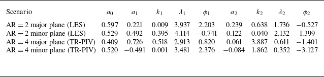


 Open access

