2.1 High-frequency waves

We now remove the rapidly varying, high-frequency part of the signal by the standard substitution $\unicode[STIX]{x1D719}\rightarrow \unicode[STIX]{x1D719}(\boldsymbol{r},t)\exp (-\text{i}\unicode[STIX]{x1D714}_{0}t)$ , with $\unicode[STIX]{x1D714}_{0}$ being the carrier wave frequency. When $|\unicode[STIX]{x2202}\unicode[STIX]{x1D719}/\unicode[STIX]{x2202}t|\ll |\unicode[STIX]{x1D714}_{0}\,\unicode[STIX]{x1D719}|$ we obtain

(2.3) $$\begin{eqnarray}\left(\text{i}\frac{\unicode[STIX]{x2202}}{\unicode[STIX]{x2202}t}+\frac{1}{2}\frac{\unicode[STIX]{x1D710}^{2}}{\unicode[STIX]{x1D714}_{\text{pe}}}\unicode[STIX]{x1D6FB}^{2}\right)\unicode[STIX]{x1D6FB}^{2}\unicode[STIX]{x1D719}-\frac{1}{2}\frac{\unicode[STIX]{x1D714}_{\text{ce}}^{2}}{\unicode[STIX]{x1D714}_{\text{pe}}}\unicode[STIX]{x1D6FB}_{\bot }^{2}\unicode[STIX]{x1D719}=\frac{1}{2}\unicode[STIX]{x1D714}_{\text{pe}}\unicode[STIX]{x1D735}\boldsymbol{\cdot }\left(\frac{\overline{n}}{n_{0}}\unicode[STIX]{x1D735}\unicode[STIX]{x1D719}\right).\end{eqnarray}$$

We explicitly use $\unicode[STIX]{x1D714}_{0}\approx \unicode[STIX]{x1D714}_{\text{uh}}\approx \unicode[STIX]{x1D714}_{\text{pe}}$ as appropriate for weakly magnetized plasmas (Krasnosel’skikh & Sotnikov Reference Krasnosel’skikh and Sotnikov1977), with $\unicode[STIX]{x1D714}_{\text{ce}}\ll \unicode[STIX]{x1D714}_{\text{pe}}$ . In this limit the nonlinear frequency shift (Kadomtsev & Karpman Reference Kadomtsev and Karpman1971) is due to a change in the local bulk plasma density induced by the wave nonlinearity. The model (2.3) is often used, but can be generalized to include the effect also of the low-frequency convection of the high-frequency wave field (Volokitin & Krafft Reference Volokitin and Krafft2005).

One consequence of the magnetic field is that the group velocity $\boldsymbol{u}_{g}$ is in general no longer parallel to the wave vector. This has implications for the filamentation instability, in particular.

2.2 Equations for the low-frequency density variations

We now relate the variations of the high-frequency potential to the slow variations in plasma density. The simplest relation relevant here assumes that ponderomotive forces associated with the spatial variation of the high-frequency wave field sets the electrons into slow bulk motions. The resulting charge imbalance gives rise to slowly varying electric fields that sets also the ion component into motion.

2.2.1 Average force relations

Averaging the electron momentum over the fast time scale $\unicode[STIX]{x1D714}_{\text{pe}}^{-1}$ we obtain an expression for the balance between the electrostatic force, the electron pressure force and the Miller force (or radiation pressure from the Langmuir waves (Kono, Škorić & ter Haar Reference Kono, Škorić and ter Haar1980)). We thus have a simplified linear expression for the quasi-equilibrium of electrons at temperature $T_{e}$ in the electrostatic and Miller force potentials as

(2.4) $$\begin{eqnarray}\unicode[STIX]{x1D735}(en_{0}\overline{\unicode[STIX]{x1D719}}-T_{e}\overline{n}-{\textstyle \frac{1}{2}}\unicode[STIX]{x1D700}_{0}|\unicode[STIX]{x1D735}\unicode[STIX]{x1D719}|^{2})=0.\end{eqnarray}$$

The ion equations of motion give a relation between $\overline{\unicode[STIX]{x1D719}}$ and the quasi-neutral plasma density $\overline{n}$ which finally gives a relation between $\overline{n}/n_{0}$ and $|\unicode[STIX]{x1D735}\unicode[STIX]{x1D719}|^{2}$ .

2.2.2 Ion fluid models

For consistency we require the ion dynamics to be described by magnetized models as well. First we use a simple cold ion fluid model to identify the basic wave modes entering the problem. Since we consider weak magnetic fields, we assume $\unicode[STIX]{x1D6FA}_{\text{ci}}<\unicode[STIX]{x1D6FA}_{\text{pi}}$ , in terms of ion cyclotron and ion plasma frequency, respectively. It is well known that the dispersion relation for such a model can be written as

(2.5) $$\begin{eqnarray}\unicode[STIX]{x1D714}^{2}(\unicode[STIX]{x1D714}^{2}-\unicode[STIX]{x1D6FA}_{\text{ci}}^{2})-C_{s}^{2}(k_{\bot }^{2}\unicode[STIX]{x1D714}^{2}+k_{\Vert }^{2}(\unicode[STIX]{x1D714}^{2}-\unicode[STIX]{x1D6FA}_{\text{ci}}^{2}))=0.\end{eqnarray}$$

We identify two dispersion relations: a high-frequency part $\unicode[STIX]{x1D714}>\unicode[STIX]{x1D6FA}_{\text{ci}}$ and a low-frequency part $\unicode[STIX]{x1D714}<\unicode[STIX]{x1D6FA}_{\text{ci}}$ . As limiting cases we recognize ion sound waves $\unicode[STIX]{x1D714}=C_{s}k_{\Vert }$ along magnetic field lines and ion cyclotron waves $\unicode[STIX]{x1D714}=\sqrt{\unicode[STIX]{x1D6FA}_{\text{ci}}^{2}+C_{s}^{2}k_{\bot }^{2}}$ propagating in the direction perpendicular to the magnetic field lines. The two branches have particular interest for decay of the high-frequency electron waves by opening for an ion wave decay product in addition to the standard ion sound waves. For $k_{\bot }=0$ we also have the ion cyclotron resonance at $\unicode[STIX]{x1D714}=\unicode[STIX]{x1D6FA}_{\text{ci}}$ .

Linearizing the basic equations, with the assumption of a simple equilibrium state, with constant plasma density $n_{0}$ and homogeneous magnetic fields $\boldsymbol{B}_{0}$ , the set of equations are then reduced to the ion continuity equation

(2.6) $$\begin{eqnarray}\frac{\unicode[STIX]{x2202}}{\unicode[STIX]{x2202}t}\overline{n}=-n_{0}\unicode[STIX]{x1D735}\boldsymbol{\cdot }\overline{\boldsymbol{u}}=-n_{0}\unicode[STIX]{x1D735}_{\bot }\boldsymbol{\cdot }\overline{\boldsymbol{u}}-n_{0}\frac{\unicode[STIX]{x2202}\overline{u}_{\Vert }}{\unicode[STIX]{x2202}z},\end{eqnarray}$$

and the ion momentum equation

(2.7) $$\begin{eqnarray}n_{0}M\frac{\unicode[STIX]{x2202}}{\unicode[STIX]{x2202}t}\overline{\boldsymbol{u}}=-\unicode[STIX]{x1D6FE}T_{i}\unicode[STIX]{x1D735}\overline{n}-en_{0}(\unicode[STIX]{x1D735}\overline{\unicode[STIX]{x1D719}}-\overline{\boldsymbol{u}}\times \boldsymbol{B}_{0}),\end{eqnarray}$$

for singly charged ions, where we have used the ideal gas law for the ion equation of state, $p_{i}=T_{i}n$ . With $C_{s}^{2}=(\unicode[STIX]{x1D6FE}T_{i}+T_{e})/M$ , we find (Dysthe et al. Reference Dysthe, Mjølhus, Pécseli and Stenflo1978) the equation relating the low-frequency density variation

(2.8) $$\begin{eqnarray}\displaystyle & & \displaystyle \left(\frac{\unicode[STIX]{x2202}^{4}}{\unicode[STIX]{x2202}t^{4}}-C_{s}^{2}\unicode[STIX]{x1D6FB}^{2}\frac{\unicode[STIX]{x2202}^{2}}{\unicode[STIX]{x2202}t^{2}}-C_{s}^{2}\unicode[STIX]{x1D6FA}_{\text{ci}}^{2}\frac{\unicode[STIX]{x2202}^{2}}{\unicode[STIX]{x2202}z^{2}}+\unicode[STIX]{x1D6FA}_{\text{ci}}^{2}\frac{\unicode[STIX]{x2202}^{2}}{\unicode[STIX]{x2202}t^{2}}\right)\frac{\overline{n}}{n_{0}}\nonumber\\ \displaystyle & & \displaystyle \quad =\frac{1}{4}\frac{\unicode[STIX]{x1D700}_{0}}{n_{0}M}\left(\unicode[STIX]{x1D6FB}^{2}\frac{\unicode[STIX]{x2202}^{2}|\unicode[STIX]{x1D735}\unicode[STIX]{x1D719}|^{2}}{\unicode[STIX]{x2202}t^{2}}+\unicode[STIX]{x1D6FA}_{\text{ci}}^{2}\frac{\unicode[STIX]{x2202}^{2}|\unicode[STIX]{x1D735}\unicode[STIX]{x1D719}|^{2}}{\unicode[STIX]{x2202}z^{2}}\right),\end{eqnarray}$$

which reproduces the linear dispersion relation (2.5) if we set $|\unicode[STIX]{x1D735}\unicode[STIX]{x1D719}|^{2}=0$ .

We note that finite ion temperatures enter only through the sound speed $C_{s}$ in (2.8). Without any significant loss of generality we may thus set $T_{i}=0$ in the present fluid model, which gives a slight advantage for the ensuing normalizations. By the use of a fluid model for the ions, we ignore nonlinear Landau damping (Dysthe & Pécseli Reference Dysthe and Pécseli1977; Shatashvili & Tsintsadze Reference Shatashvili and Tsintsadze1982; Melrose Reference Melrose1987) and also a nonlinear ion cyclotron damping (Dysthe & Pécseli Reference Dysthe and Pécseli1978). Collisional effects can be important for the ion dynamics in some laboratory experiments and also in the ionospheric E-region. These effects have been considered by Pécseli et al. (Reference Pécseli, Rasmussen, Tagare and Thomsen1986), Faria & Shukla (Reference Faria and Shukla1999), Shukla & Farid (Reference Shukla and Farid1999) and Shukla, Eliasson & Stenflo (Reference Shukla, Eliasson and Stenflo2003), for instance. Collisional effects have at times been used to ‘mimic’ the effect of ion Landau damping.

The model for the low-frequency dynamics is thus electrostatic, and will not account for excitation of magnetosonic waves (Shukla et al. Reference Shukla, Eliasson and Stenflo2003), for instance. Such couplings can be relevant for large scale phenomena, in the Earth’s ionosphere or magnetosphere. We also recall that at long wavelengths, the ion cyclotron waves have an electromagnetic component which is here ignored. The limitations of the low-frequency dynamics will be discussed in more detail in § 6.

3.1 The nonlinear frequency shift

For later use we introduce $\unicode[STIX]{x1D6FA}_{H}(\boldsymbol{K})$ by the definition $\unicode[STIX]{x1D6FC}_{H}(\boldsymbol{K},\unicode[STIX]{x1D6FA}_{H}(\boldsymbol{K}))=0$ so that

(3.6) $$\begin{eqnarray}\unicode[STIX]{x1D6FC}_{H}(\boldsymbol{K},\unicode[STIX]{x1D6FA})\equiv K^{2}[\unicode[STIX]{x1D6FA}-\unicode[STIX]{x1D6FA}_{H}(\boldsymbol{K})].\end{eqnarray}$$

For a modified (or renormalized) version of $\unicode[STIX]{x1D6FC}_{H}(\boldsymbol{K},\unicode[STIX]{x1D6FA})$ we introduce similarly the symbol $\unicode[STIX]{x1D6FC}(\boldsymbol{K},\unicode[STIX]{x1D6FA})$ without subscript as

(3.7) $$\begin{eqnarray}\displaystyle \unicode[STIX]{x1D6FC}(\boldsymbol{K},\unicode[STIX]{x1D6FA})\equiv \unicode[STIX]{x1D6FC}_{H}(\boldsymbol{K},\unicode[STIX]{x1D6FA})-\frac{\unicode[STIX]{x1D714}_{\text{pe}}}{2}K^{2}\langle \overline{\unicode[STIX]{x1D702}}\rangle & \equiv & \displaystyle K^{2}[\unicode[STIX]{x1D6FA}-\unicode[STIX]{x1D6FA}_{H}(\boldsymbol{K})-\unicode[STIX]{x0394}\unicode[STIX]{x1D6FA}_{H}]\nonumber\\ \displaystyle & = & \displaystyle \unicode[STIX]{x1D6FC}_{H}(\boldsymbol{K},\unicode[STIX]{x1D6FA}-\unicode[STIX]{x0394}\unicode[STIX]{x1D6FA}_{H}),\end{eqnarray}$$

with a frequency shift $\unicode[STIX]{x0394}\unicode[STIX]{x1D6FA}_{H}\equiv (1/2)\unicode[STIX]{x1D714}_{\text{pe}}\langle \overline{\unicode[STIX]{x1D702}}\rangle$ , where $\overline{\unicode[STIX]{x1D702}}$ is real but otherwise unspecified for the moment. Using (3.2) we have

(3.8) $$\begin{eqnarray}\displaystyle & & \displaystyle \unicode[STIX]{x1D6FC}(\boldsymbol{K}_{1}-\boldsymbol{K},\unicode[STIX]{x1D6FA}_{1}-\unicode[STIX]{x1D6FA})\langle \unicode[STIX]{x1D719}(\boldsymbol{K}_{1},\unicode[STIX]{x1D6FA}_{1})\unicode[STIX]{x1D719}^{\ast }(\boldsymbol{K}_{1}-\boldsymbol{K},\unicode[STIX]{x1D6FA}_{1}-\unicode[STIX]{x1D6FA})\rangle \nonumber\\ \displaystyle & & \displaystyle \quad =\frac{\unicode[STIX]{x1D714}_{\text{pe}}}{2}\int \text{d}\boldsymbol{K}_{2}\int \text{d}\unicode[STIX]{x1D6FA}_{2}(\boldsymbol{K}_{1}-\boldsymbol{K})\boldsymbol{\cdot }(\boldsymbol{K}_{1}-\boldsymbol{K}-\boldsymbol{K}_{2})\left(\frac{\langle \overline{n}^{\ast }(\boldsymbol{K}_{2},\unicode[STIX]{x1D6FA}_{2})\rangle }{n_{0}}-\langle \overline{\unicode[STIX]{x1D702}}\rangle \unicode[STIX]{x1D6FF}(\boldsymbol{K}_{2})\unicode[STIX]{x1D6FF}(\unicode[STIX]{x1D6FA}_{2})\right)\nonumber\\ \displaystyle & & \displaystyle \qquad \times \,\langle \unicode[STIX]{x1D719}(\boldsymbol{K}_{1},\unicode[STIX]{x1D6FA}_{1})\unicode[STIX]{x1D719}^{\ast }(\boldsymbol{K}_{1}-\boldsymbol{K}-\boldsymbol{K}_{2},\unicode[STIX]{x1D6FA}_{1}-\unicode[STIX]{x1D6FA}-\unicode[STIX]{x1D6FA}_{2})\rangle .\end{eqnarray}$$

When obtaining (3.8) we have approximated the ensemble average of a product by the product of the averages, as in other related studies (Pécseli Reference Pécseli2014; Kono & Pécseli Reference Kono and Pécseli2016).

The wave vector–frequency structure function $\langle \unicode[STIX]{x1D719}(\boldsymbol{K}_{1},\unicode[STIX]{x1D6FA}_{1})\unicode[STIX]{x1D719}^{\ast }(\boldsymbol{K}_{2},\unicode[STIX]{x1D6FA}_{2})\rangle$ can be expanded as

(3.9) $$\begin{eqnarray}\displaystyle \langle \unicode[STIX]{x1D719}(\boldsymbol{K}_{1},\unicode[STIX]{x1D6FA}_{1})\unicode[STIX]{x1D719}^{\ast }(\boldsymbol{K}_{2},\unicode[STIX]{x1D6FA}_{2})\rangle & = & \displaystyle I_{0}(\boldsymbol{K}_{1},\unicode[STIX]{x1D6FA}_{1})\unicode[STIX]{x1D6FF}(\boldsymbol{K}_{1}-\boldsymbol{K}_{2})\unicode[STIX]{x1D6FF}(\unicode[STIX]{x1D6FA}_{1}-\unicode[STIX]{x1D6FA}_{2})\nonumber\\ \displaystyle & & \displaystyle +\,I_{1}\!\left(\!\frac{\boldsymbol{K}_{1}-\boldsymbol{K}_{2}}{2},\frac{\unicode[STIX]{x1D6FA}_{1}-\unicode[STIX]{x1D6FA}_{2}}{2};\boldsymbol{K}_{1}+\boldsymbol{K}_{2},\unicode[STIX]{x1D6FA}_{1}+\unicode[STIX]{x1D6FA}_{2}\!\right)+\cdots \,.\end{eqnarray}$$

The lowest-order homogeneous and stationary spectrum is given as $I_{0}(\boldsymbol{K}_{1},\unicode[STIX]{x1D6FA}_{1})$ while $I_{1}((\boldsymbol{K}_{1}-\boldsymbol{K}_{2})/2,(\unicode[STIX]{x1D6FA}_{1}-\unicode[STIX]{x1D6FA}_{2})/2;\boldsymbol{K}_{1}+\boldsymbol{K}_{2},\unicode[STIX]{x1D6FA}_{1}+\unicode[STIX]{x1D6FA}_{2})$ is its first-order inhomogeneous and non-stationary perturbation. Then the left- and right-hand sides of (3.8) are rewritten to give

(3.10) $$\begin{eqnarray}\displaystyle & & \displaystyle \unicode[STIX]{x1D6FC}(\boldsymbol{K}_{1}-\boldsymbol{K},\unicode[STIX]{x1D6FA}_{1}-\unicode[STIX]{x1D6FA})\langle \unicode[STIX]{x1D719}(\boldsymbol{K}_{1},\unicode[STIX]{x1D6FA}_{1})\unicode[STIX]{x1D719}^{\ast }(\boldsymbol{K}_{1}-\boldsymbol{K},\unicode[STIX]{x1D6FA}_{1}-\unicode[STIX]{x1D6FA})\rangle \nonumber\\ \displaystyle & & \displaystyle \quad =\unicode[STIX]{x1D6FC}(\boldsymbol{K}_{1}-\boldsymbol{K},\unicode[STIX]{x1D6FA}_{1}-\unicode[STIX]{x1D6FA})\left\{I_{0}(\boldsymbol{K}_{1},\unicode[STIX]{x1D6FA}_{1})\unicode[STIX]{x1D6FF}(\boldsymbol{K})\unicode[STIX]{x1D6FF}(\unicode[STIX]{x1D6FA})\right.\nonumber\\ \displaystyle & & \displaystyle \qquad +\left.I_{1}\left(\boldsymbol{K}_{1}-\frac{\boldsymbol{K}}{2},\unicode[STIX]{x1D6FA}_{1}-\frac{\unicode[STIX]{x1D6FA}}{2};\boldsymbol{K},\unicode[STIX]{x1D6FA}\right)+\cdots \,\!\right\}\nonumber\\ \displaystyle & & \displaystyle \quad =\frac{\unicode[STIX]{x1D714}_{\text{pe}}}{2}\int \text{d}\boldsymbol{K}_{2}\int \text{d}\unicode[STIX]{x1D6FA}_{2}(\boldsymbol{K}_{1}-\boldsymbol{K})\boldsymbol{\cdot }(\boldsymbol{K}_{1}-\boldsymbol{K}-\boldsymbol{K}_{2})\left(\frac{\langle \overline{n}^{\ast }(\boldsymbol{K}_{2},\unicode[STIX]{x1D6FA}_{2})\rangle }{n_{0}}-\langle \overline{\unicode[STIX]{x1D702}}\rangle \unicode[STIX]{x1D6FF}(\boldsymbol{K}_{2})\unicode[STIX]{x1D6FF}(\unicode[STIX]{x1D6FA}_{2})\right)\nonumber\\ \displaystyle & & \displaystyle \qquad \times \,\left\{I_{0}(\boldsymbol{K}_{1},\unicode[STIX]{x1D6FA}_{1})\unicode[STIX]{x1D6FF}(\boldsymbol{K}_{2}+\boldsymbol{K})\unicode[STIX]{x1D6FF}(\unicode[STIX]{x1D6FA}_{2}+\unicode[STIX]{x1D6FA})\right.\nonumber\\ \displaystyle & & \displaystyle \qquad +\left.I_{1}\left(\boldsymbol{K}_{1}-\frac{\boldsymbol{K}+\boldsymbol{K}_{2}}{2},\unicode[STIX]{x1D6FA}_{1}-\frac{\unicode[STIX]{x1D6FA}+\unicode[STIX]{x1D6FA}_{2}}{2};\boldsymbol{K}+\boldsymbol{K}_{2},\unicode[STIX]{x1D6FA}+\unicode[STIX]{x1D6FA}_{2}\right)+\cdots \,\!\right\},\end{eqnarray}$$

leading to

(3.11) $$\begin{eqnarray}\unicode[STIX]{x1D6FC}(\boldsymbol{K}_{1},\unicode[STIX]{x1D6FA}_{1})I_{0}(\boldsymbol{K}_{1},\unicode[STIX]{x1D6FA}_{1})=0,\end{eqnarray}$$

(3.12) $$\begin{eqnarray}\displaystyle & & \displaystyle \unicode[STIX]{x1D6FC}(\boldsymbol{K}_{1}-\boldsymbol{K},\unicode[STIX]{x1D6FA}_{1}-\unicode[STIX]{x1D6FA})I_{1}\left(\boldsymbol{K}_{1}-\frac{\boldsymbol{K}}{2},\unicode[STIX]{x1D6FA}_{1}-\frac{\unicode[STIX]{x1D6FA}}{2};\boldsymbol{K},\unicode[STIX]{x1D6FA}\right)\nonumber\\ \displaystyle & & \displaystyle \quad =\frac{\unicode[STIX]{x1D714}_{\text{pe}}}{2}\boldsymbol{K}_{1}\boldsymbol{\cdot }(\boldsymbol{K}_{1}-\boldsymbol{K})\left(\frac{\langle \overline{n}^{\ast }(\boldsymbol{K}_{2},\unicode[STIX]{x1D6FA}_{2})\rangle }{n_{0}}-\langle \overline{\unicode[STIX]{x1D702}}\rangle \unicode[STIX]{x1D6FF}(\boldsymbol{K}_{2})\unicode[STIX]{x1D6FF}(\unicode[STIX]{x1D6FA}_{2})\right)I_{0}(\boldsymbol{K}_{1},\unicode[STIX]{x1D6FA}_{1}).\end{eqnarray}$$

From (3.11) we get

(3.13) $$\begin{eqnarray}I_{0}(\boldsymbol{K},\unicode[STIX]{x1D6FA})=G(\boldsymbol{K})\unicode[STIX]{x1D6FF}(\unicode[STIX]{x1D6FA}-\widehat{\unicode[STIX]{x1D6FA}}_{H}(\boldsymbol{K})),\end{eqnarray}$$

where $\widehat{\unicode[STIX]{x1D6FA}}_{H}(\boldsymbol{K})$ is defined similarly to $\unicode[STIX]{x1D6FA}_{H}(\boldsymbol{K})$ through $\unicode[STIX]{x1D6FC}(\boldsymbol{K},\widehat{\unicode[STIX]{x1D6FA}}_{H}(\boldsymbol{K}))=0$ . We thus find the reasonable result that, to lowest-order, the nonlinear frequency shift can be incorporated into the linear dispersion relation without otherwise affecting the wave-vector power spectrum of the waves.

Inserting to lowest order $\langle \unicode[STIX]{x1D719}(\boldsymbol{K}_{1},\unicode[STIX]{x1D6FA}_{1})\unicode[STIX]{x1D719}^{\ast }(\boldsymbol{K}_{2},\unicode[STIX]{x1D6FA}_{2})\rangle \approx I_{0}(\boldsymbol{K}_{1},\unicode[STIX]{x1D6FA}_{1})\unicode[STIX]{x1D6FF}(\boldsymbol{K}_{1}-\boldsymbol{K}_{2})\unicode[STIX]{x1D6FF}(\unicode[STIX]{x1D6FA}_{1}-\unicode[STIX]{x1D6FA}_{2})$ in (3.3) we obtain

(3.14) $$\begin{eqnarray}\langle \overline{n}(\boldsymbol{K},\unicode[STIX]{x1D6FA})\rangle =\frac{\unicode[STIX]{x1D700}_{0}}{2M\unicode[STIX]{x1D6FC}_{L}(\boldsymbol{K},\unicode[STIX]{x1D6FA})}\int \text{d}\boldsymbol{K}_{1}\int \text{d}\unicode[STIX]{x1D6FA}_{1}\boldsymbol{K}_{\mathbf{1}}\boldsymbol{\cdot }(\boldsymbol{K}_{\mathbf{1}}-\boldsymbol{K})I_{0}(\boldsymbol{K}_{1},\unicode[STIX]{x1D6FA}_{1})\unicode[STIX]{x1D6FF}(\boldsymbol{K})\unicode[STIX]{x1D6FF}(\unicode[STIX]{x1D6FA}),\end{eqnarray}$$

which by Fourier transform as in (3.1) gives $\langle \overline{n}(\boldsymbol{r},t)\rangle$ and thereby $\langle \overline{\unicode[STIX]{x1D702}}\rangle$ that enters the nonlinear frequency shift to give

(3.15) $$\begin{eqnarray}\unicode[STIX]{x0394}\unicode[STIX]{x1D6FA}_{H}=-\frac{\unicode[STIX]{x1D700}_{0}\unicode[STIX]{x1D714}_{\text{pe}}}{4MC_{s}^{2}}\int \text{d}\boldsymbol{K}\int \text{d}\unicode[STIX]{x1D6FA}K^{2}I_{0}(\boldsymbol{K},\unicode[STIX]{x1D6FA}).\end{eqnarray}$$

We have used $\unicode[STIX]{x1D700}_{L}(0,0)=-C_{s}^{2}$ .

3.2 The nonlinear dispersion relation

Substituting (3.12) into the right-hand side of (3.3) we obtain the dispersion relation

(3.16) $$\begin{eqnarray}\unicode[STIX]{x1D6FC}_{L}(\boldsymbol{K},\unicode[STIX]{x1D6FA})=\frac{\unicode[STIX]{x1D700}_{0}\unicode[STIX]{x1D714}_{\text{pe}}}{4n_{0}M}\int \text{d}\boldsymbol{K}_{1}\int \text{d}\unicode[STIX]{x1D6FA}_{1}\frac{[\boldsymbol{K}_{1}\boldsymbol{\cdot }(\boldsymbol{K}_{1}-\boldsymbol{K})]^{2}}{\unicode[STIX]{x1D6FC}(\boldsymbol{K}_{1}-\boldsymbol{K},\unicode[STIX]{x1D6FA}_{1}-\unicode[STIX]{x1D6FA})}I_{0}(\boldsymbol{K}_{1},\unicode[STIX]{x1D6FA}_{1}),\end{eqnarray}$$

giving

(3.17) $$\begin{eqnarray}\unicode[STIX]{x1D6FC}_{L}(\boldsymbol{K},\unicode[STIX]{x1D6FA})=\frac{\unicode[STIX]{x1D700}_{0}\unicode[STIX]{x1D714}_{\text{pe}}}{4n_{0}M}\int \text{d}\boldsymbol{K}_{1}\frac{[\boldsymbol{K}_{1}\boldsymbol{\cdot }(\boldsymbol{K}_{1}-\boldsymbol{K})]^{2}}{\unicode[STIX]{x1D6FC}_{H}(\boldsymbol{K}_{1}-\boldsymbol{K},\unicode[STIX]{x1D6FA}_{H}(\boldsymbol{K}_{1})-\unicode[STIX]{x1D6FA})}G(\boldsymbol{K}_{1}),\end{eqnarray}$$

where we have used (3.13) to give

(3.18) $$\begin{eqnarray}\int \text{d}\unicode[STIX]{x1D6FA}_{1}\frac{I_{0}(\boldsymbol{K}_{1},\unicode[STIX]{x1D6FA}_{1})}{\unicode[STIX]{x1D6FC}(\boldsymbol{K}_{1}-\boldsymbol{K},\unicode[STIX]{x1D6FA}_{1}-\unicode[STIX]{x1D6FA})}=\frac{G(\boldsymbol{K}_{1})}{\unicode[STIX]{x1D6FC}_{H}(\boldsymbol{K}_{1}-\boldsymbol{K},\unicode[STIX]{x1D6FA}_{H}(\boldsymbol{K}_{1})-\unicode[STIX]{x1D6FA})}.\end{eqnarray}$$

The analytical expression for $G(\boldsymbol{K})$ is not specified by our analysis. For a saturated turbulent state it can be determined experimentally, for instance (Vyacheslavov et al. Reference Vyacheslavov, Burmasov, Kandaurov, Kruglyakov, Meshkov and Sanin1995). The spectrum $I_{0}(\boldsymbol{K},\unicode[STIX]{x1D6FA})$ refers to the potential fluctuations: the electric field power spectrum ${\mathcal{E}}_{0}(\boldsymbol{K},\unicode[STIX]{x1D6FA})=K^{2}I_{0}(\boldsymbol{K},\unicode[STIX]{x1D6FA})$ can be introduced if desired.

Because of (3.18), the nonlinear frequency shift included in (3.13) is of little consequence here and is not considered in the following analysis.

4.1 Normalizations

For presenting normalized variables we introduce the normalizations:

1. (i) frequency $\unicode[STIX]{x1D6FA}^{\prime }\equiv (3/2)(\unicode[STIX]{x1D6FA}/\unicode[STIX]{x1D6FA}_{\text{pi}})\sqrt{M/m}$ ,

2. (ii) wave numbers $\boldsymbol{K}^{\prime }\equiv (3/2)\boldsymbol{K}\unicode[STIX]{x1D706}_{\text{De}}\sqrt{M/m}$ and also $\boldsymbol{K}_{0}^{\prime }\equiv (3/2)\boldsymbol{K}_{0}\unicode[STIX]{x1D706}_{\text{De}}\sqrt{M/m}$ ,

3. (iii) wave energy density is normalized by $((1/2)\unicode[STIX]{x1D700}_{0}A_{0}^{2}/n_{0}T_{e})(3/2)(M/m),$

where $^{\prime }$ will denote normalized quantities throughout, and not differentiations. For other purposes (Krasnosel’skikh & Sotnikov Reference Krasnosel’skikh and Sotnikov1977) it can be advantageous to use different normalizations for directions along and transverse to magnetic field lines, but we see no advantage of that here, given the need of resolving both sound-like and ion cyclotron wave forms for the low-frequency perturbations.

We let the parameter $\unicode[STIX]{x1D701}^{2}\equiv (M/m)(\unicode[STIX]{x1D714}_{\text{ce}}/\unicode[STIX]{x1D714}_{\text{pe}})^{2}(3/2)^{2}$ measure the strength of the magnetic field and find in terms of the normalized units

(4.1) $$\begin{eqnarray}\displaystyle \unicode[STIX]{x1D6FC}_{H}(\boldsymbol{K}^{\prime },\unicode[STIX]{x1D6FA}^{\prime }) & \equiv & \displaystyle \left[\left(\unicode[STIX]{x1D6FA}^{\prime }-K^{\prime 2}\right)K^{\prime 2}-\frac{1}{3}\unicode[STIX]{x1D701}^{2}K_{\bot }^{\prime 2}\right]\left(\frac{2}{3}\right)^{3}\left(\frac{m}{M}\right)^{3/2}\frac{\unicode[STIX]{x1D6FA}_{\text{pi}}}{\unicode[STIX]{x1D706}_{\text{De}}^{2}}\nonumber\\ \displaystyle & \equiv & \displaystyle \left(\frac{2}{3}\right)^{3}\left(\frac{m}{M}\right)^{3/2}\frac{\unicode[STIX]{x1D6FA}_{\text{pi}}}{\unicode[STIX]{x1D706}_{\text{De}}^{2}}\unicode[STIX]{x1D6FC}_{H}^{\prime }(\boldsymbol{K}^{\prime },\unicode[STIX]{x1D6FA}^{\prime }),\end{eqnarray}$$

and

(4.2) $$\begin{eqnarray}\displaystyle \unicode[STIX]{x1D6FC}_{L}(\boldsymbol{K}^{\prime },\unicode[STIX]{x1D6FA}^{\prime }) & \equiv & \displaystyle \frac{\displaystyle \left(\unicode[STIX]{x1D6FA}^{\prime 2}-\frac{m}{M}\unicode[STIX]{x1D701}^{2}\right)(\unicode[STIX]{x1D6FA}^{\prime 2}-K^{\prime 2})-\frac{m}{M}\unicode[STIX]{x1D701}^{2}K_{\bot }^{\prime 2}}{\displaystyle \left(\unicode[STIX]{x1D6FA}^{\prime 2}-\frac{m}{M}\unicode[STIX]{x1D701}^{2}\right)K^{\prime 2}+\frac{m}{M}\unicode[STIX]{x1D701}^{2}K_{\bot }^{\prime 2}}(\unicode[STIX]{x1D706}_{\text{De}}^{2}\unicode[STIX]{x1D6FA}_{\text{pi}}^{2})\nonumber\\ \displaystyle & \equiv & \displaystyle \unicode[STIX]{x1D6FA}_{\text{pi}}^{2}\unicode[STIX]{x1D706}_{\text{De}}^{2}\unicode[STIX]{x1D6FC}_{L}^{\prime }(\boldsymbol{K}^{\prime },\unicode[STIX]{x1D6FA}^{\prime }),\end{eqnarray}$$

where $\unicode[STIX]{x1D6FC}_{H}^{\prime }(\boldsymbol{K}^{\prime },\unicode[STIX]{x1D6FA}^{\prime })$ and $\unicode[STIX]{x1D6FC}_{L}^{\prime }(\boldsymbol{K}^{\prime },\unicode[STIX]{x1D6FA}^{\prime })$ are dimensionless.

If we require $\unicode[STIX]{x1D701}\sim O(1)$ , implying $\unicode[STIX]{x1D714}_{\text{ce}}/\unicode[STIX]{x1D714}_{\text{pe}}\sim \sqrt{m/M}$ , we find that the magnetic field has small influence on the overall ion dynamics. From this it is however not possible to draw the conclusion that we can ignore the ion magnetization altogether. There is a low-frequency range $\unicode[STIX]{x1D6FA}^{\prime }\in \{0,\unicode[STIX]{x1D701}\sqrt{m/M}\}$ which is accessible for instance for decay. If we set $\unicode[STIX]{x1D701}\sqrt{m/M}=0$ in (4.2) we will find that two $\unicode[STIX]{x1D6FA}^{\prime 2}$ value’s cancel and this wave mode disappears from the analysis. The structure of the equations is then changed. We also note that all wavenumber components appear squared: this imposes some symmetry conditions on the results.

4.2 Normalized dispersion relations

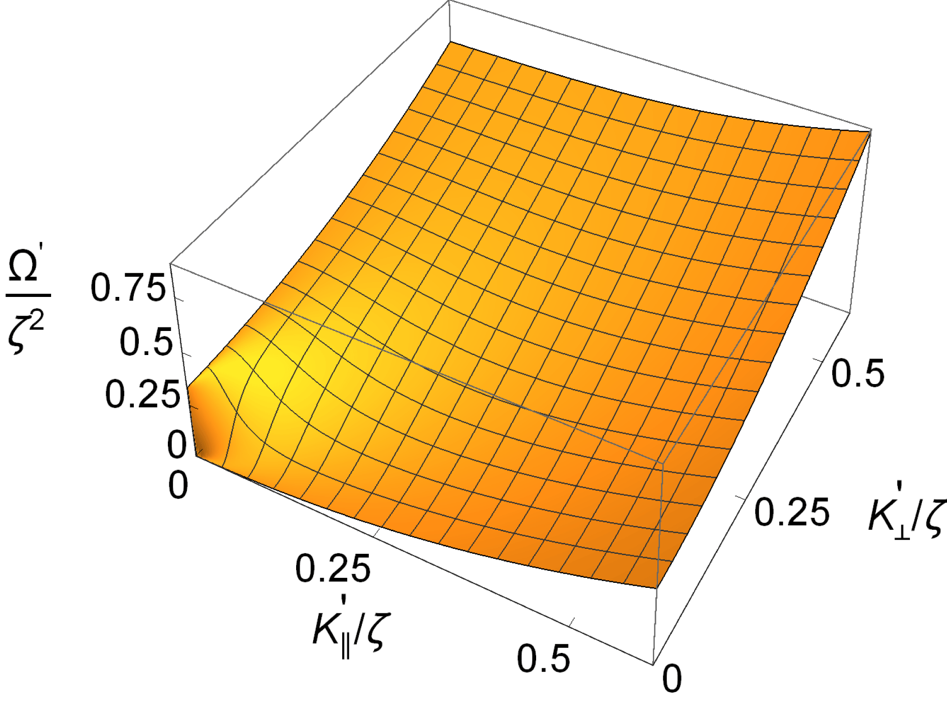
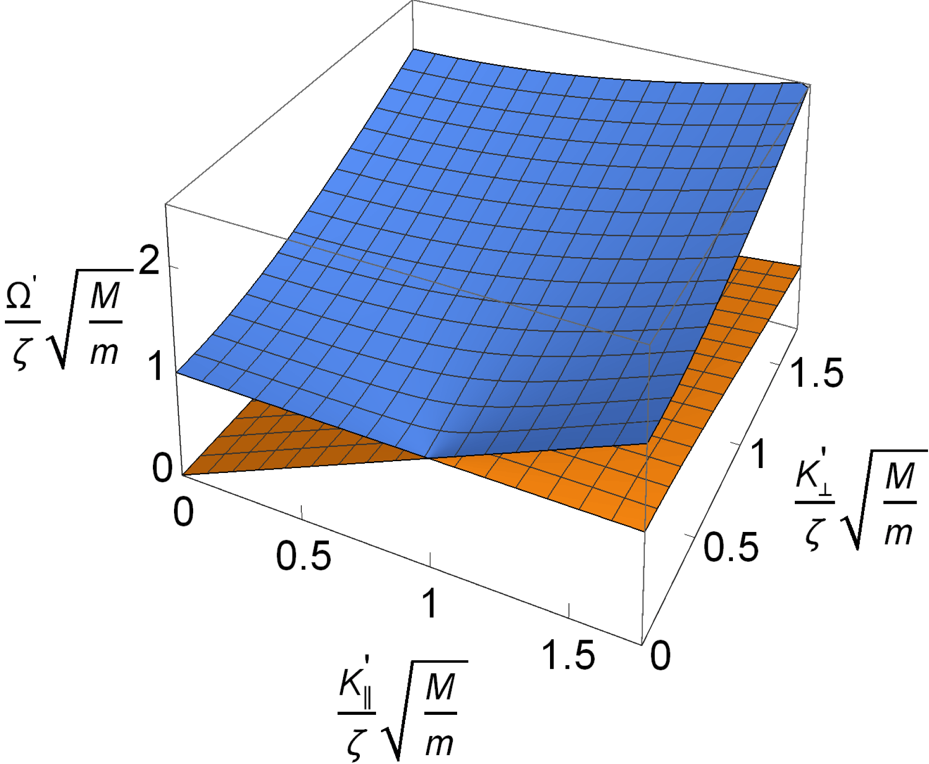
The two wave modes relevant for the present study, electron plasma waves and ion sound and cyclotron waves, are illustrated in figures 1 and 2 using the normalized units. We note that for the electron waves, the effects of the magnetic field are important for $K^{\prime }/\unicode[STIX]{x1D701}<1$ ; for larger wavenumbers the difference compared to the unmagnetized Langmuir wave case become small. Similarly, we find the magnetic field to be important for the ion dynamics only for normalized frequencies $\unicode[STIX]{x1D6FA}^{\prime }$ of the order of $\unicode[STIX]{x1D701}\sqrt{m/M}$ or smaller. The relevance of lower hybrid waves will be discussed in § 6.

Figure 1.

The approximate electron wave dispersion relation for weakly magnetized plasmas, here shown in normalized units, $\unicode[STIX]{x1D6FA}^{\prime }=K^{\prime 2}+(1/3)\unicode[STIX]{x1D701}^{2}K_{\bot }^{\prime 2}/K^{\prime 2}$ . Recall that the basic reference frequency $\unicode[STIX]{x1D714}_{\text{pe}}$ has been subtracted.

Figure 2.

Ion wave dispersion relation in normalized units for weakly magnetized plasmas where $\unicode[STIX]{x1D6FA}_{\text{ci}}<\unicode[STIX]{x1D6FA}_{\text{pi}}$ , see (2.5).

With these normalizations the dispersion relation (3.17) is reduced to

(4.3) $$\begin{eqnarray}\unicode[STIX]{x1D6FC}_{L}^{\prime }(\boldsymbol{K}^{\prime },\unicode[STIX]{x1D6FA}^{\prime })=\int \text{d}\boldsymbol{K}_{1}^{\prime }\frac{[\boldsymbol{K}_{1}^{\prime }\boldsymbol{\cdot }(\boldsymbol{K}_{1}^{\prime }-\boldsymbol{K}^{\prime })]^{2}G(\boldsymbol{K}_{1}^{\prime })}{\unicode[STIX]{x1D6FC}_{H}^{\prime }(\boldsymbol{K}_{1}^{\prime }-\boldsymbol{K}^{\prime },\unicode[STIX]{x1D6FA}_{H}^{\prime }(\boldsymbol{K}_{1}^{\prime })-\unicode[STIX]{x1D6FA}^{\prime })}.\end{eqnarray}$$

Here $\boldsymbol{K}^{\prime }$ and $\unicode[STIX]{x1D6FA}^{\prime }$ can be replaced by $-\boldsymbol{K}^{\prime }$ and $-\unicode[STIX]{x1D6FA}^{\prime }$ to give

(4.4) $$\begin{eqnarray}\unicode[STIX]{x1D6FC}_{L}^{\prime }(-\boldsymbol{K}^{\prime },-\unicode[STIX]{x1D6FA}^{\prime })=\int \text{d}\boldsymbol{K}_{1}^{\prime }[\boldsymbol{K}_{1}^{\prime }\boldsymbol{\cdot }(\boldsymbol{K}_{1}^{\prime }+\boldsymbol{K}^{\prime })]^{2}\left\{\frac{G(\boldsymbol{K}_{1}^{\prime })}{\unicode[STIX]{x1D6FC}_{H}^{\prime }(\boldsymbol{K}_{1}^{\prime }+\boldsymbol{K}^{\prime },\unicode[STIX]{x1D6FA}_{H}^{\prime }(\boldsymbol{K}_{1}^{\prime })+\unicode[STIX]{x1D6FA}^{\prime })}\right\}.\end{eqnarray}$$

Noting $\unicode[STIX]{x1D6FC}_{L}^{\prime }(-\boldsymbol{K}^{\prime },-\unicode[STIX]{x1D6FA}^{\prime })=\unicode[STIX]{x1D6FC}_{L}^{\prime }(\boldsymbol{K}^{\prime },\unicode[STIX]{x1D6FA}^{\prime })$ , we rewrite (4.3) as

(4.5) $$\begin{eqnarray}\displaystyle \unicode[STIX]{x1D6FC}_{L}^{\prime }(\boldsymbol{K}^{\prime },\unicode[STIX]{x1D6FA}^{\prime }) & = & \displaystyle \frac{1}{2}\int \text{d}\boldsymbol{K}_{1}^{\prime }\left\{\frac{[\boldsymbol{K}_{1}^{\prime }\boldsymbol{\cdot }(\boldsymbol{K}_{1}^{\prime }-\boldsymbol{K}^{\prime })]^{2}}{\unicode[STIX]{x1D6FC}_{H}^{\prime }(\boldsymbol{K}_{1}^{\prime }-\boldsymbol{K}^{\prime },\unicode[STIX]{x1D6FA}_{H}^{\prime }(\boldsymbol{K}_{1}^{\prime })-\unicode[STIX]{x1D6FA}^{\prime })}\right.\nonumber\\ \displaystyle & & \displaystyle +\left.\frac{[\boldsymbol{K}_{1}^{\prime }\boldsymbol{\cdot }(\boldsymbol{K}_{1}^{\prime }+\boldsymbol{K}^{\prime })]^{2}}{\unicode[STIX]{x1D6FC}_{H}^{\prime }(\boldsymbol{K}_{1}^{\prime }+\boldsymbol{K}^{\prime },\unicode[STIX]{x1D6FA}_{H}^{\prime }(\boldsymbol{K}_{1}^{\prime })+\unicode[STIX]{x1D6FA}^{\prime })}\right\}G(\boldsymbol{K}_{1}^{\prime }).\end{eqnarray}$$

The latter symmetric form is best suited for describing modulational instabilities. The present § 4.2 summarizes the main analytical results of our study. In the following we illustrate some of the properties of the results.

4.3 Single mode analysis

A plane wave can be seen as a limiting case of a very narrow spectrum. This limit can be analysed by taking $G(\boldsymbol{K}^{\prime })=A_{0}^{2}\unicode[STIX]{x1D6FF}(\boldsymbol{K}^{\prime }-\boldsymbol{K}_{0}^{\prime })$ in (4.5). Even though this is a limiting particular case, it seems that even these results are only sparsely covered by the literature (Dysthe et al. Reference Dysthe, Mjølhus, Pécseli and Stenflo1978; Freund & Papadopoulos Reference Freund and Papadopoulos1980), so we summarize some selected cases here. Analytical results can be obtained, but they are too long to be reproduced. Instead we show some illustrative results.

Figure 3.

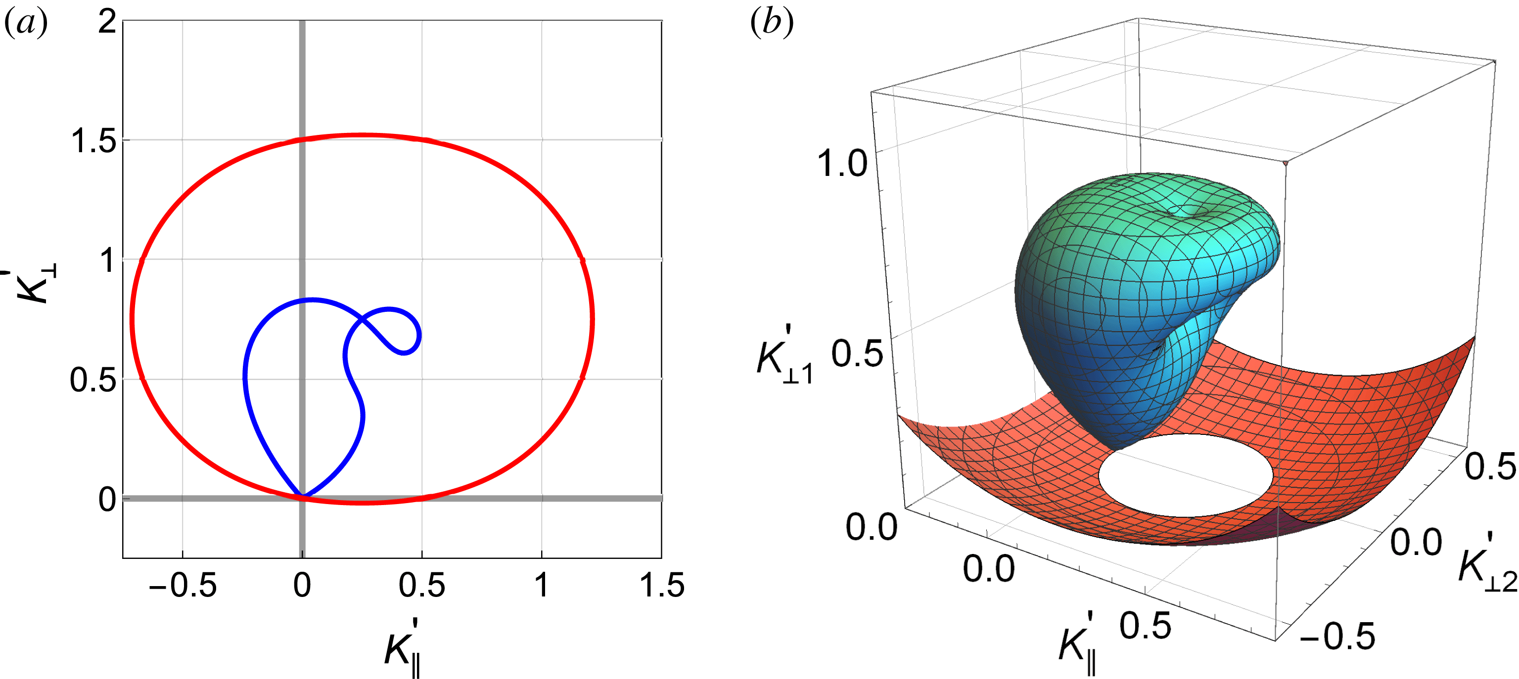
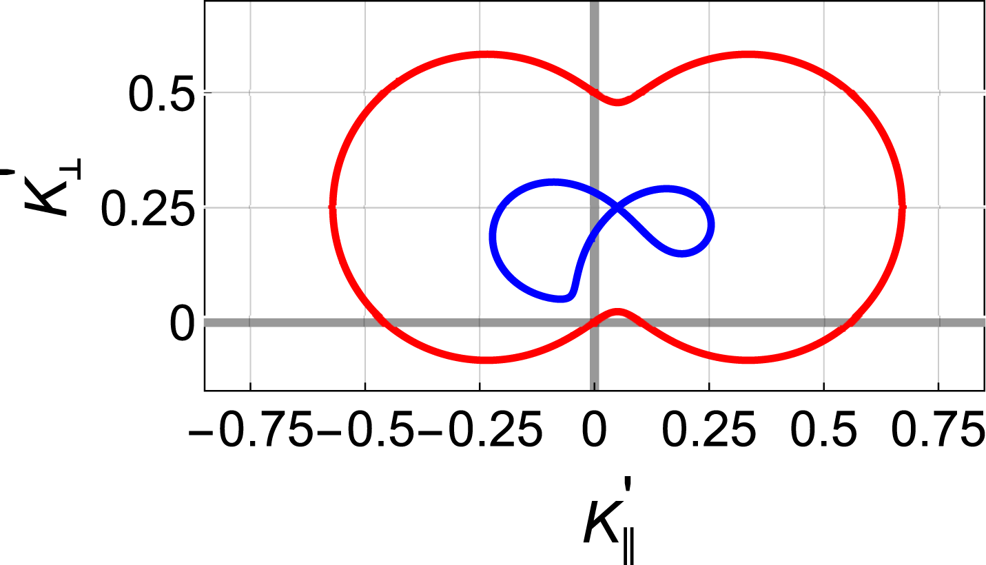
Illustration of the possible wave vectors of the ion waves participating in the decay of electron plasma waves. The nearly elliptical curve corresponds to the low-frequency branch in figure 2, the other curve to the high-frequency branch in that figure. The present illustration has $\boldsymbol{K}_{0}^{\prime }\equiv \{K_{0\Vert }^{\prime },0,K_{0\bot }^{\prime }\}=\{0.25,0,0.75\}$ in normalized units. For illustration we use $\unicode[STIX]{x1D701}=1$ and a mass ratio of $M/m=1600$ . Figure (a) represents a cut at $K_{\bot 2}^{\prime }=0$ in the fully three-dimensional figure (b). The two components of $\boldsymbol{K}_{\bot }^{\prime }$ are denoted $K_{\bot 1}^{\prime }$ and $K_{\bot 2}^{\prime }$ on this figure.

4.3.1 Parametric decay

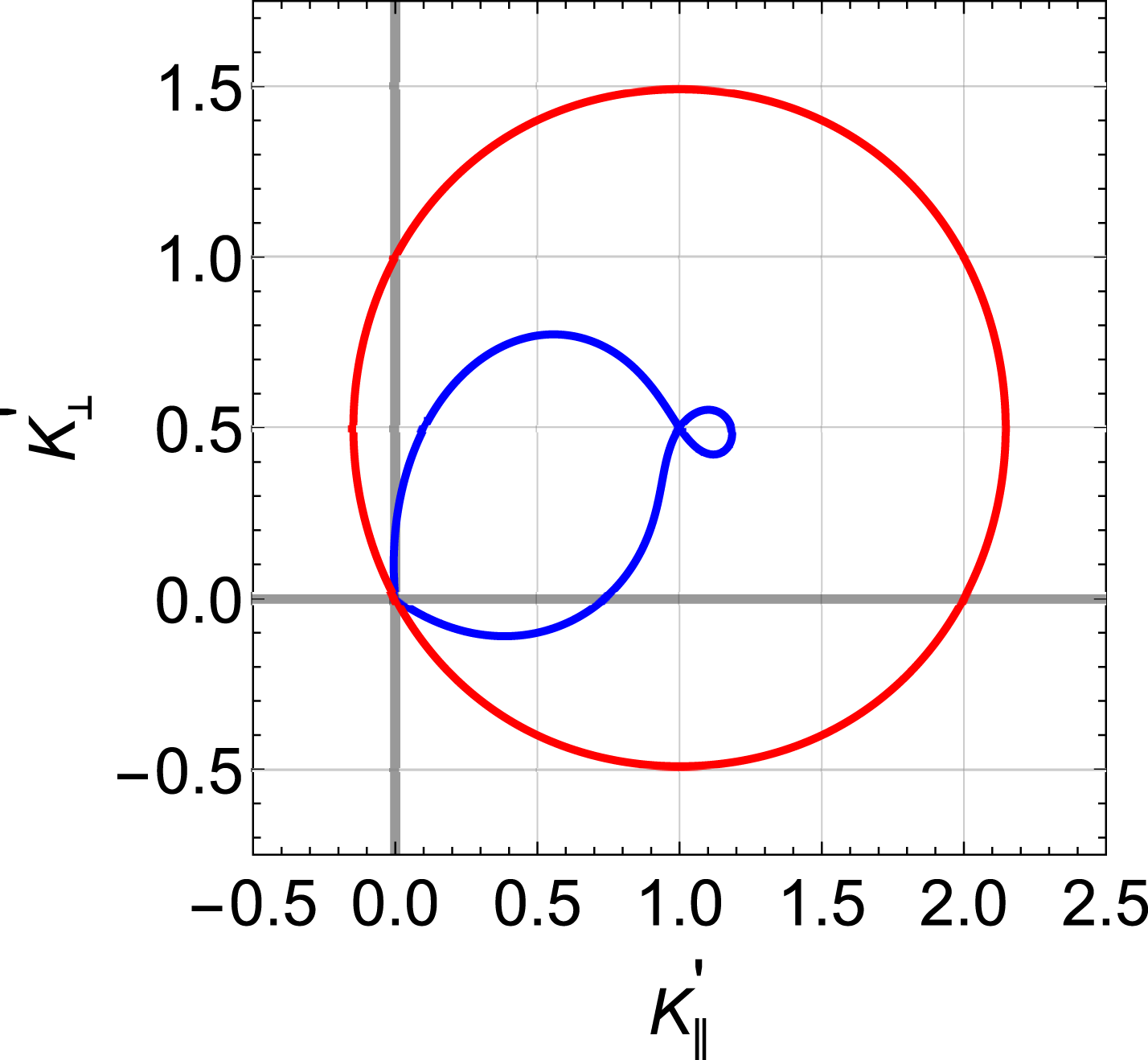
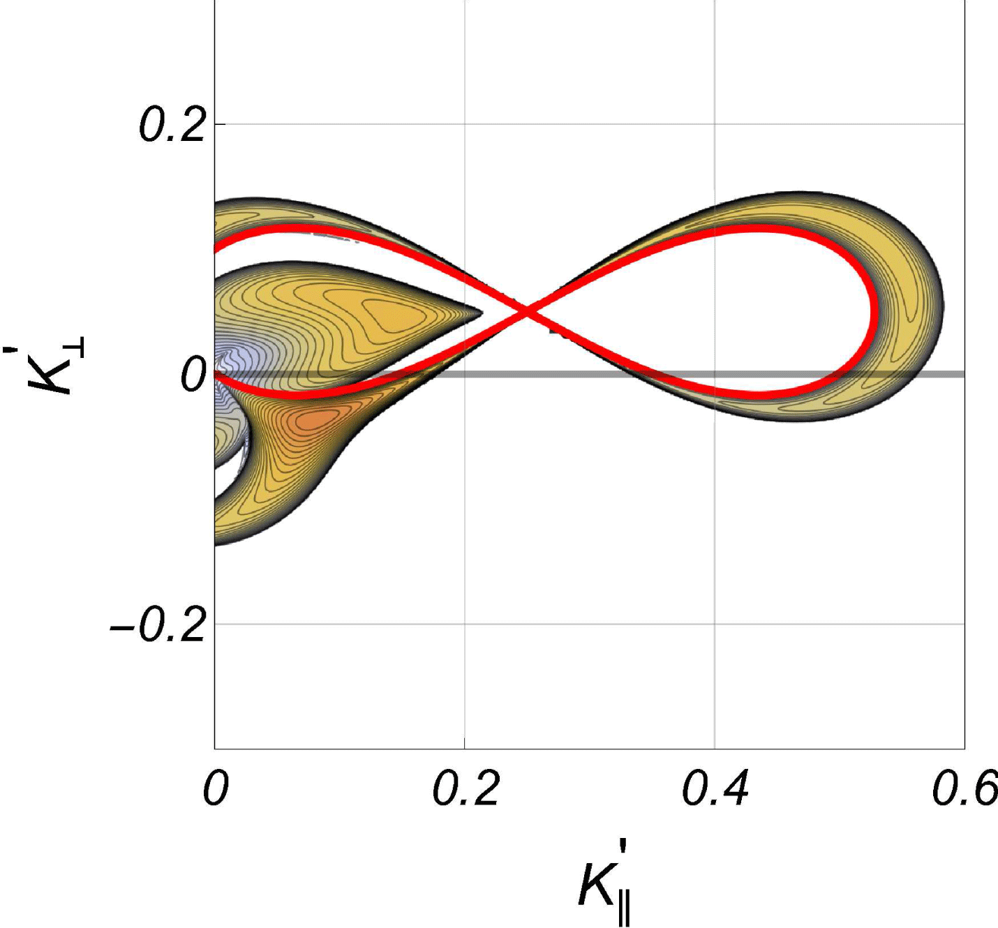
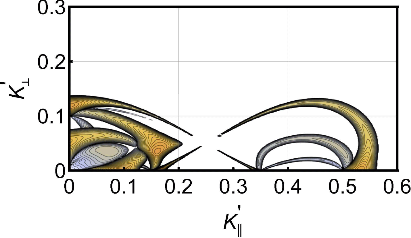
One basic nonlinear wave phenomenon accounted for by our basic relation (4.5) is the decay of electron plasma waves to another electron plasma wave and one of the ion wave branches seen in figure 2, the process subject to wavenumber and frequency matching conditions. In figures 3 and 4 we show two examples for the wave vectors of the ion waves participating in such a decay, given an initial plane electron plasma wave with wavenumber $\boldsymbol{K}_{0}^{\prime }$ , where the corresponding frequency $\unicode[STIX]{x1D6FA}_{0}$ is found from the dispersion relation, see for instance figure 1. The corresponding values for the electron plasma ‘daughter’ wave is found by the wavenumber matching conditions. It is instructive to compare these result with those found for the simpler Langmuir wave decay in unmagnetized plasmas (Kono & Pécseli Reference Kono and Pécseli2016). As a reminder of the three-dimensional nature of the problem, we inserted in figure 3 a presentation of a part of the ion wave decay vectors in a fully three-dimensional wave vector space. It is important to note that the possibility of decay does not imply that the decay will actually occur, and also we will in general have a decay rate that varies along the curves.

Figure 4.

Illustration of the possible wave vectors of the ion waves participating in the decay of electron plasma waves, to be compared with figure 3. The present illustration has $\boldsymbol{K}_{0}^{\prime }=\{1.0,0,0.5\}$ in normalized units. The figure represents a cut in a three-dimensional presentation as in figure 3.

Figure 5.

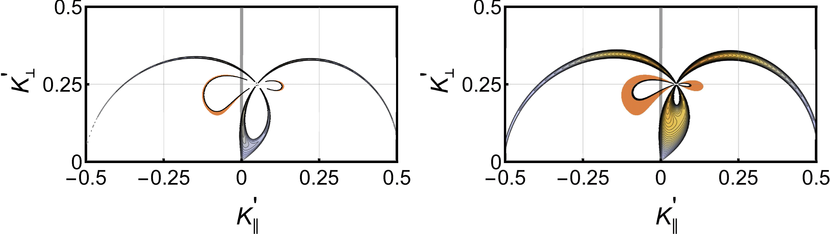
Illustration of the normalized growth rate for the parametric decay corresponding to figure 3 for the case where $A_{0}^{2}=0.005$ , see also figure 4. The maximum contour level for the growth rate is here $\text{Im}\{\unicode[STIX]{x1D6FA}^{\prime }\}=0.025$ in normalized units. We take $\unicode[STIX]{x1D701}=1$ .

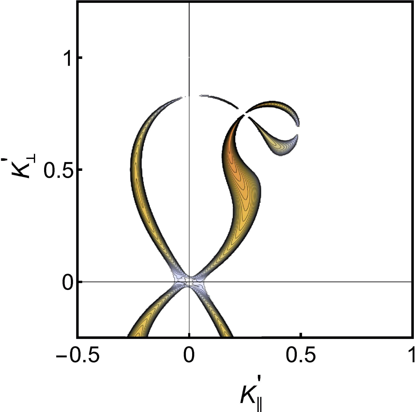
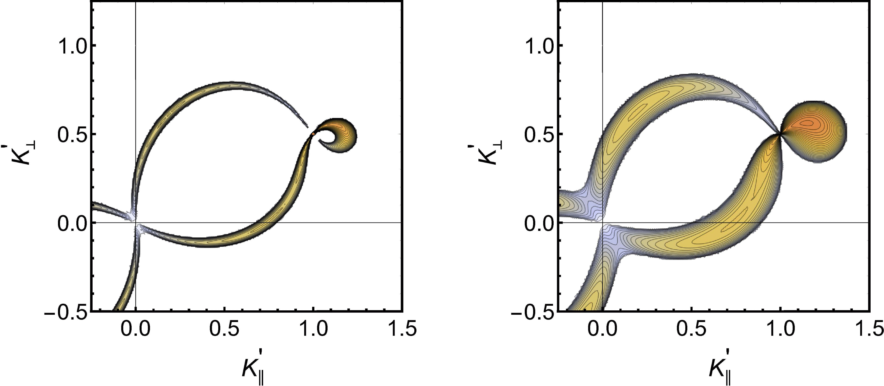
Solutions of the growth rate derived from the dispersion relation are shown in figures 5 and 6 for a selected set of parameters. Most of the relevant information is found in the plane spanned by $\boldsymbol{B}_{0}$ and $\boldsymbol{K}_{0}^{\prime }$ . Only the imaginary part $\text{Im}\{\unicode[STIX]{x1D6FA}^{\prime }\}$ is shown as the information in the real part is comparatively less important. In figures 5 and 6 we readily recognize the inner curve from figure 3, but there seems to be no decay to the outer elliptical branch. We found that this is due to the weak magnetic field limit considered in the present analysis. If we reduce the mass ratio to an artificially small number we find that also this branch becomes excited. A supplementary figure 7 shows results for a different carrier wave vector $\boldsymbol{K}_{0}^{\prime }$ .

Figure 6.

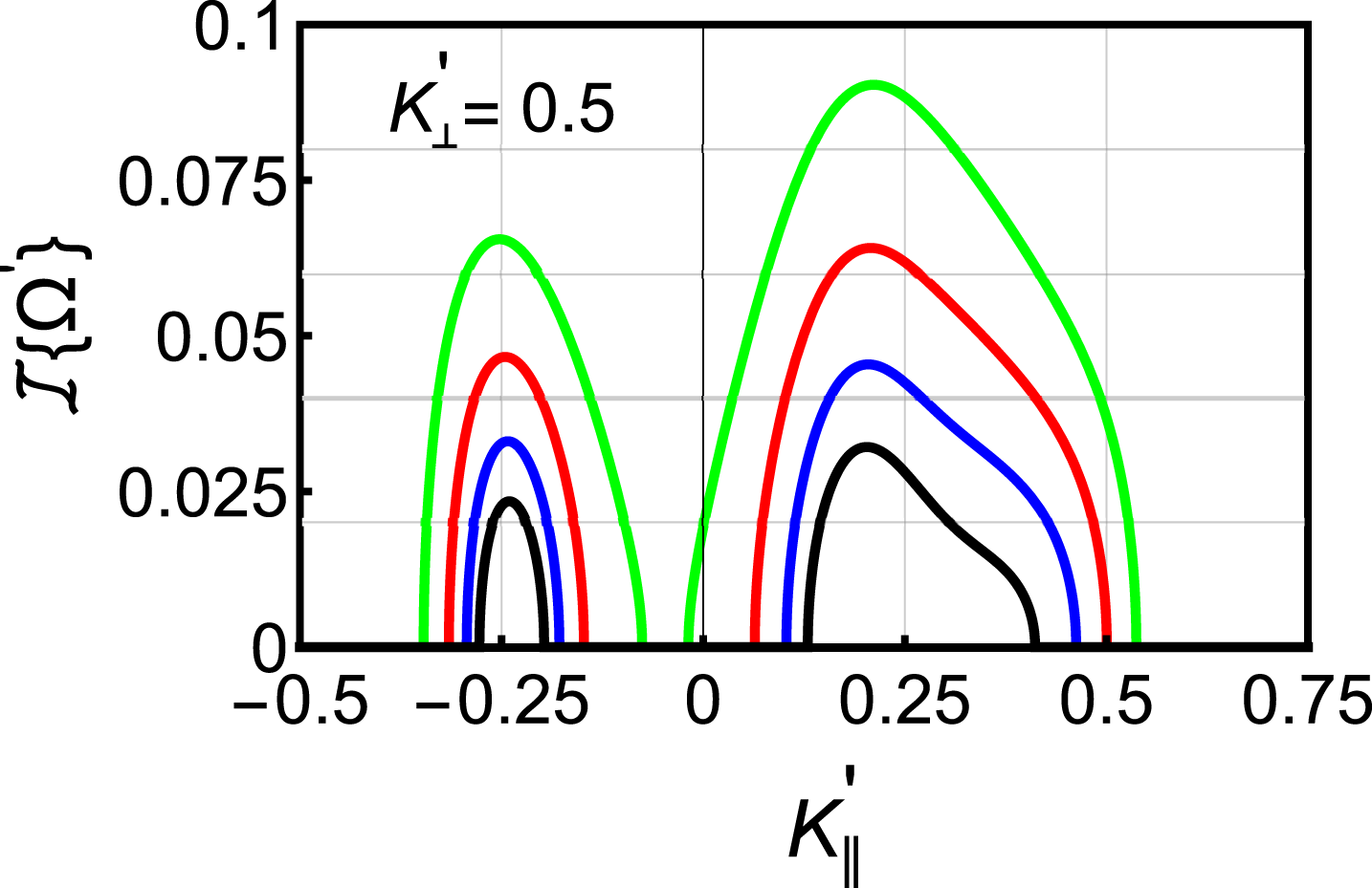
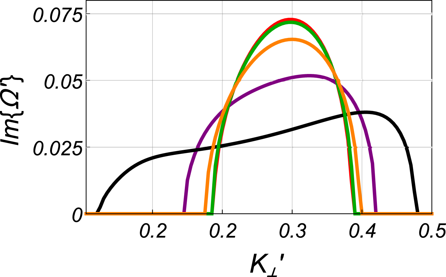
Illustration of the growth rate for varying $K_{\Vert }^{\prime }$ , and selected amplitudes, here $A_{0}^{2}=0.0125,0.025,0.05,0.1$ sampled at a constant $K_{\bot }^{\prime }=0.5$ , i.e. along a horizontal line in figure 5. The parameters correspond otherwise to those in figure 5. The peak value of the growth rate scales as $A_{0}$ to a good approximation. We find the same scaling for the width, at least for small $A_{0}$ .

Figure 7.

Illustrations of the growth rate for the parametric decay corresponding to figure 4 for two amplitudes, $A_{0}^{2}=0.005$ and $A_{0}^{2}=0.05$ . The maximum contour levels are 0.05 and 0.15, respectively, in normalized units.

In particular, in figure 6 we show the variation of local peak value of the normalized growth rate $\text{Im}\{\unicode[STIX]{x1D6FA}^{\prime }\}$ for selected amplitudes $A_{0}^{2}$ , for a fixed value of $K_{\bot }^{\prime }$ . To a good approximation we find the variation $\text{Im}\{\unicode[STIX]{x1D6FA}^{\prime }\}\sim A_{0}$ for $A_{0}^{2}\leqslant 0.5$ for this and other examples studied. The result is consistent with what is found for the unmagnetized case (Thornhill & ter Haar Reference Thornhill and ter Haar1978; Kono & Pécseli Reference Kono and Pécseli2016). The figure also illustrates the nonlinear line broadening for increasing $A_{0}^{2}$ . Enhancing the wave amplitude further than the range shown on the figure we find the two modes of propagation to merge into one broad line. The decay curves in figures 3 and 4 are curves in a three-dimensional wave vector space. Due to the finite bandwidth, the growth rates illustrated in figures 5–7 represent ‘cuts’ in a three-dimensional volume in a wave vector space. The same comment applies to a number of figures in the following.

4.3.2 Modulational instability

The results presented so far refer to parametric decay of electron plasma waves. The frequency and wave vector matching condition is here sufficient to give the contours for the decay, and only the growth rate of the decay instability needs to be determined. Modulational instabilities are of a different nature. This is a four wave process, and the decay product is no longer a wave mode satisfying a dispersion relation. Our dispersion relation (4.5) accounts for both decay and modulational instabilities.

For unmagnetized waves in the small amplitude limit the separation between decay and modulational instabilities is straight forward, at least as long as a fluid model is used. The point is here that modulational instabilities are found when the perturbations in plasma density is in counter-phase with the spatial variation of $|E|^{2}$ . This happens when a wave packet or a spatially modulated wavetrain propagates at a speed below $C_{s}$ . With the normalization used here this conditions implies $K^{\prime }<1/2$ for modulational instabilities in unmagnetized plasmas. The sign of the phase relation (in phase or counter-phase) is in this case given be the sign of $u_{g}^{2}-C_{s}^{2}$ , where $u_{g}$ is the group velocity of the Langmuir wave. The finite line width for increasing amplitudes ‘blurs’ the separation between modulational and decay instabilities (Kono & Pécseli Reference Kono and Pécseli2016). Similarly, a kinetic ion model will imply a complex relationship between perturbations in plasma density and the Miller force, and also in this case the range of decay and modulational instability will overlap.

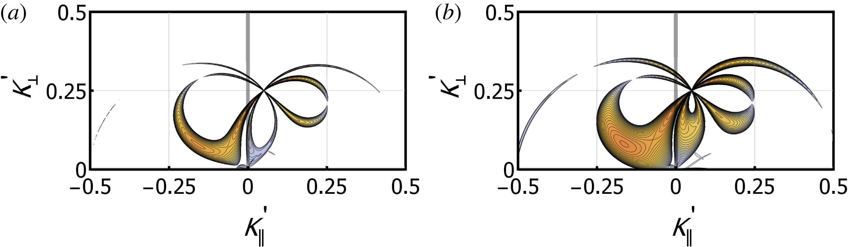
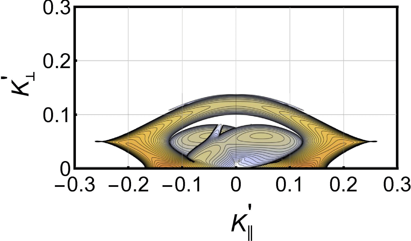
For magnetized plasmas the topology of the problem can in general be more complicated (Dysthe et al. Reference Dysthe, Mjølhus, Pécseli and Stenflo1978; Dysthe & Pécseli Reference Dysthe and Pécseli1978), and now contains too many parameters to allow presentation in a simple diagram. We present here an example where $\boldsymbol{K}_{0}^{\prime }=\{0.05,0,0.25\}$ in normalized units, see figure 8. For reference we show in figure 9 the decay products for theses parameters. We recognize in figure 8 the decay to the high-frequency ion branch, but find also here that the decay to the low-frequency branch is absent. In addition we find in figure 8 a growth rate for another mode type, the modulational instability. We thus find here a coexistence of decay and modulational instabilities. This coexistence has no counterpart in fluid models of unmagnetized weakly nonlinear electron plasma waves, as mentioned. We found that the growth rates for fixed $A_{0}^{2}$ become significantly reduced when the magnitude of wavenumber of the ‘mother wave’ is reduced. This feature is readily explained by noting that $A_{0}^{2}$ is the mean square of the potential of the electrostatic wave field, while it is the electric field that enters the nonlinear driving term, $E_{0}^{2}=(K_{0}A_{0})^{2}$ .

Figure 8.

Illustration of a case with coexistence of parametric decay and modulational instability for $\boldsymbol{K}_{0}^{\prime }=\{0.05,0,0.25\}$ with two amplitudes $A_{0}^{2}=0.1$ and $A_{0}^{2}=0.5$ . A small wavenumber component $K_{0\Vert }^{\prime }=0.05$ is included to break the symmetry. The maximum contours shown are at $\text{Im}\{\unicode[STIX]{x1D6FA}^{\prime }\}=0.015$ and $\text{Im}\{\unicode[STIX]{x1D6FA}^{\prime }\}=0.03$ in (a) and (b), respectively.

Figure 9.

Decay diagram for the case where $\boldsymbol{K}_{0}^{\prime }=\{0.05,0,0.25\}$ , see also figure 8.

In order to give analytical estimates for the growth rates of the modulational instabilities we rewrite the dispersion relation by introducing

(4.6) $$\begin{eqnarray}\unicode[STIX]{x1D6FA}_{L\pm }^{\prime }(\boldsymbol{K}^{\prime })\equiv \frac{1}{\sqrt{2}}\sqrt{K^{\prime ^{2}}+\frac{m}{M}\unicode[STIX]{x1D701}^{2}\pm \sqrt{\frac{m^{2}}{M^{2}}\unicode[STIX]{x1D701}^{4}+K^{\prime 4}-2\frac{m}{M}\unicode[STIX]{x1D701}^{2}(K^{\prime ^{2}}-2K_{\bot }^{\prime 2})}},\end{eqnarray}$$

and

(4.7) $$\begin{eqnarray}\unicode[STIX]{x1D6FA}_{H}^{\prime }(\boldsymbol{K}^{\prime })\equiv K^{\prime 2}+\frac{1}{3}\unicode[STIX]{x1D701}^{2}\frac{K_{\bot }^{\prime 2}}{K^{\prime 2}},\end{eqnarray}$$

and we can for instance write $\unicode[STIX]{x1D6FC}_{H}^{\prime }(\boldsymbol{K}^{\prime },\unicode[STIX]{x1D6FA}^{\prime })=[\unicode[STIX]{x1D6FA}^{\prime }-\unicode[STIX]{x1D6FA}_{H}^{\prime }(\boldsymbol{K}^{\prime })]K^{\prime 2}$ , see figure 1 for illustration. We use also the abbreviation $\unicode[STIX]{x1D6FA}_{0}^{\prime }(\boldsymbol{K}^{\prime })\equiv \sqrt{(m/M)\unicode[STIX]{x1D701}^{2}K_{\bot }^{\prime 2}/K^{\prime 2}}$ . With this notation we can write the dispersion relation for the perturbation of one single mode $A_{0}^{2}\unicode[STIX]{x1D6FF}(\boldsymbol{K}^{\prime }-\boldsymbol{K}_{0}^{\prime })$ as

(4.8) $$\begin{eqnarray}\displaystyle & & \displaystyle \frac{(\unicode[STIX]{x1D6FA}^{\prime 2}-\unicode[STIX]{x1D6FA}_{L-}^{\prime 2}(\boldsymbol{K}^{\prime }))(\unicode[STIX]{x1D6FA}^{\prime 2}-\unicode[STIX]{x1D6FA}_{L+}^{\prime 2}(\boldsymbol{K}^{\prime }))}{\displaystyle \unicode[STIX]{x1D6FA}^{\prime 2}-\frac{m}{M}\unicode[STIX]{x1D701}^{2}+\unicode[STIX]{x1D6FA}_{0}^{\prime 2}(\boldsymbol{K}^{\prime })}\nonumber\\ \displaystyle & & \displaystyle \quad =A_{0}^{2}\frac{K^{\prime 2}}{2}\left(\frac{[\boldsymbol{K}_{0}^{\prime }\boldsymbol{\cdot }(\boldsymbol{K}_{0}^{\prime }-\boldsymbol{K}^{\prime })]^{2}}{(\boldsymbol{K}_{0}^{\prime }-\boldsymbol{K}^{\prime })^{2}}\frac{1}{\unicode[STIX]{x1D6FA}_{H}^{\prime }(\boldsymbol{K}_{0}^{\prime })-\unicode[STIX]{x1D6FA}^{\prime }-\unicode[STIX]{x1D6FA}_{H}^{\prime }(\boldsymbol{K}_{0}^{\prime }-\boldsymbol{K}^{\prime })}\right.\nonumber\\ \displaystyle & & \displaystyle \qquad +\left.\frac{[\boldsymbol{K}_{0}^{\prime }\boldsymbol{\cdot }(\boldsymbol{K}_{0}^{\prime }+\boldsymbol{K}^{\prime })]^{2}}{(\boldsymbol{K}_{0}^{\prime }+\boldsymbol{K}^{\prime })^{2}}\frac{1}{\unicode[STIX]{x1D6FA}_{H}^{\prime }(\boldsymbol{K}_{0}^{\prime })+\unicode[STIX]{x1D6FA}^{\prime }-\unicode[STIX]{x1D6FA}_{H}^{\prime }(\boldsymbol{K}_{0}^{\prime }+\boldsymbol{K}^{\prime })}\right).\end{eqnarray}$$

We can rewrite (4.8) as

(4.9) $$\begin{eqnarray}\displaystyle & & \displaystyle (\unicode[STIX]{x1D6FA}^{\prime }+\unicode[STIX]{x1D6FA}_{H}^{\prime }(\boldsymbol{K}_{0}^{\prime })-\unicode[STIX]{x1D6FA}_{H}^{\prime }(\boldsymbol{K}_{0}^{\prime }+\boldsymbol{K}^{\prime }))(\unicode[STIX]{x1D6FA}^{\prime }-\unicode[STIX]{x1D6FA}_{H}^{\prime }(\boldsymbol{K}_{0}^{\prime })+\unicode[STIX]{x1D6FA}_{H}^{\prime }(\boldsymbol{K}_{0}^{\prime }-\boldsymbol{K}^{\prime }))\nonumber\\ \displaystyle & & \displaystyle \quad =-A_{0}^{2}\frac{K^{\prime 2}}{2}\left(\frac{[\boldsymbol{K}_{0}^{\prime }\boldsymbol{\cdot }(\boldsymbol{K}_{0}^{\prime }-\boldsymbol{K}^{\prime })]^{2}}{(\boldsymbol{K}_{0}^{\prime }-\boldsymbol{K}^{\prime })^{2}}(\unicode[STIX]{x1D6FA}^{\prime }+\unicode[STIX]{x1D6FA}_{H}^{\prime }(\boldsymbol{K}_{0}^{\prime })-\unicode[STIX]{x1D6FA}_{H}^{\prime }(\boldsymbol{K}_{0}^{\prime }+\boldsymbol{K}^{\prime }))\right.\nonumber\\ \displaystyle & & \displaystyle \qquad -\left.\frac{[\boldsymbol{K}_{0}^{\prime }\boldsymbol{\cdot }(\boldsymbol{K}_{0}^{\prime }+\boldsymbol{K}^{\prime })]^{2}}{(\boldsymbol{K}_{0}^{\prime }+\boldsymbol{K})^{\prime 2}}(\unicode[STIX]{x1D6FA}^{\prime }-\unicode[STIX]{x1D6FA}_{H}^{\prime }(\boldsymbol{K}_{0}^{\prime })+\unicode[STIX]{x1D6FA}_{H}^{\prime }(\boldsymbol{K}_{0}^{\prime }-\boldsymbol{K}^{\prime }))\right)\nonumber\\ \displaystyle & & \displaystyle \qquad \times \,\frac{\displaystyle \unicode[STIX]{x1D6FA}^{\prime 2}-\frac{m}{M}\unicode[STIX]{x1D701}^{2}+\unicode[STIX]{x1D6FA}_{0}^{\prime 2}(\boldsymbol{K}^{\prime })}{(\unicode[STIX]{x1D6FA}^{\prime 2}-\unicode[STIX]{x1D6FA}_{L-}^{\prime 2}(\boldsymbol{K}^{\prime }))(\unicode[STIX]{x1D6FA}^{\prime 2}-\unicode[STIX]{x1D6FA}_{L+}^{\prime 2}(\boldsymbol{K}^{\prime }))}.\end{eqnarray}$$

With a little algebra we can rewrite the left-hand side of (4.9) as

(4.10) $$\begin{eqnarray}\displaystyle & & \displaystyle (\unicode[STIX]{x1D6FA}^{\prime }+\unicode[STIX]{x1D6FA}_{H}^{\prime }(\boldsymbol{K}_{0}^{\prime })-\unicode[STIX]{x1D6FA}_{H}^{\prime }(\boldsymbol{K}_{0}^{\prime }+\boldsymbol{K}^{\prime }))(\unicode[STIX]{x1D6FA}^{\prime }-\unicode[STIX]{x1D6FA}_{H}^{\prime }(\boldsymbol{K}_{0}^{\prime })+\unicode[STIX]{x1D6FA}_{H}^{\prime }(\boldsymbol{K}_{0}^{\prime }-\boldsymbol{K}^{\prime }))\nonumber\\ \displaystyle & & \displaystyle \quad =(\unicode[STIX]{x1D6FA}^{\prime }-{\textstyle \frac{1}{2}}[\unicode[STIX]{x1D6FA}_{H}^{\prime }(\boldsymbol{K}_{0}^{\prime }+\boldsymbol{K}^{\prime })-\unicode[STIX]{x1D6FA}_{H}^{\prime }(\boldsymbol{K}_{0}^{\prime }-\boldsymbol{K}^{\prime })])^{2}\nonumber\\ \displaystyle & & \displaystyle \qquad -\,(\unicode[STIX]{x1D6FA}_{H}^{\prime }(\boldsymbol{K}_{0}^{\prime })-{\textstyle \frac{1}{2}}[\unicode[STIX]{x1D6FA}_{H}^{\prime }(\boldsymbol{K}_{0}^{\prime }+\boldsymbol{K}^{\prime })+\unicode[STIX]{x1D6FA}_{H}^{\prime }(\boldsymbol{K}_{0}^{\prime }-\boldsymbol{K}^{\prime })])^{2}.\end{eqnarray}$$

As an approximation for small $|\boldsymbol{K}^{\prime }|$ we have $(1/2)(\unicode[STIX]{x1D6FA}_{H}^{\prime }(\boldsymbol{K}_{0}^{\prime }+\boldsymbol{K}^{\prime })-\unicode[STIX]{x1D6FA}_{H}^{\prime }(\boldsymbol{K}_{0}^{\prime }-\boldsymbol{K}^{\prime }))\approx \boldsymbol{K}^{\prime }\boldsymbol{\cdot }\unicode[STIX]{x1D735}_{\boldsymbol{K}^{\prime }}\unicode[STIX]{x1D6FA}_{H}^{\prime }(\boldsymbol{K}^{\prime })\equiv \boldsymbol{K}^{\prime }\boldsymbol{\cdot }\boldsymbol{u}g(\boldsymbol{K}^{\prime })$ , and similarly $(1/2)[\unicode[STIX]{x1D6FA}_{H}^{\prime }(\boldsymbol{K}_{0}^{\prime }+\boldsymbol{K}^{\prime })+\unicode[STIX]{x1D6FA}_{H}^{\prime }(\boldsymbol{K}_{0}^{\prime }-\boldsymbol{K}^{\prime })-2\unicode[STIX]{x1D6FA}_{H}^{\prime }(\boldsymbol{K}_{0}^{\prime })]\approx (1/2)\unicode[STIX]{x1D735}_{\boldsymbol{K}^{\prime }}\unicode[STIX]{x1D735}_{\boldsymbol{K}^{\prime }}\unicode[STIX]{x1D6FA}_{H}^{\prime }(\boldsymbol{K}^{\prime })\boldsymbol{ : }\boldsymbol{K}^{\prime }\boldsymbol{K}^{\prime }$ . As a first approximation we can use $\unicode[STIX]{x1D6FA}^{\prime }\approx (1/2)[\unicode[STIX]{x1D6FA}_{H}^{\prime }(\boldsymbol{K}_{0}^{\prime }+\boldsymbol{K}^{\prime })-\unicode[STIX]{x1D6FA}_{H}^{\prime }(\boldsymbol{K}_{0}^{\prime }-\boldsymbol{K}^{\prime })]$ corresponding to wave packets propagating with the group velocity without changing their shape. A slow spatial dispersion of the wave packets is accounted for by the second term. As an approximation we can now write

(4.11) $$\begin{eqnarray}\displaystyle & & \displaystyle \unicode[STIX]{x1D6FA}^{\prime }\approx {\textstyle \frac{1}{2}}[\unicode[STIX]{x1D6FA}_{H}^{\prime }(\boldsymbol{K}_{0}^{\prime }+\boldsymbol{K}^{\prime })-\unicode[STIX]{x1D6FA}_{H}^{\prime }(\boldsymbol{K}_{0}^{\prime }-\boldsymbol{K}^{\prime })]\nonumber\\ \displaystyle & & \displaystyle \quad \pm \,\sqrt{(\unicode[STIX]{x1D6FA}_{H}^{\prime }(\boldsymbol{K}_{0}^{\prime })-{\textstyle \frac{1}{2}}(\unicode[STIX]{x1D6FA}_{H}^{\prime }(\boldsymbol{K}_{0}^{\prime }+\boldsymbol{K}^{\prime })+\unicode[STIX]{x1D6FA}_{H}^{\prime }(\boldsymbol{K}_{0}^{\prime }-\boldsymbol{K}^{\prime })))^{2}-{\textstyle \frac{1}{2}}A_{0}^{2}K^{\prime 2}\unicode[STIX]{x1D6FD}(\boldsymbol{K}_{0}^{\prime },\boldsymbol{K}^{\prime })},\qquad\end{eqnarray}$$

where we have defined

(4.12) $$\begin{eqnarray}\displaystyle \unicode[STIX]{x1D6FD}(\boldsymbol{K}_{0}^{\prime },\boldsymbol{K}^{\prime }) & \equiv & \displaystyle (\unicode[STIX]{x1D6FA}_{H}^{\prime }(\boldsymbol{K}_{0}^{\prime })-\frac{1}{2}[\unicode[STIX]{x1D6FA}_{H}^{\prime }(\boldsymbol{K}_{0}^{\prime }+\boldsymbol{K}^{\prime })+\unicode[STIX]{x1D6FA}_{H}^{\prime }(\boldsymbol{K}_{0}^{\prime }-\boldsymbol{K}^{\prime })])\nonumber\\ \displaystyle & & \displaystyle \times \,\left(\frac{[\boldsymbol{K}_{0}^{\prime }\boldsymbol{\cdot }(\boldsymbol{K}_{0}^{\prime }-\boldsymbol{K}^{\prime })]^{2}}{(\boldsymbol{K}_{0}^{\prime }-\boldsymbol{K}^{\prime })^{2}}+\frac{[\boldsymbol{K}_{0}^{\prime }\boldsymbol{\cdot }(\boldsymbol{K}_{0}^{\prime }+\boldsymbol{K}^{\prime })]^{2}}{(\boldsymbol{K}_{0}^{\prime }+\boldsymbol{K}^{\prime })^{2}}\right)\nonumber\\ \displaystyle & & \displaystyle \times \,\frac{\displaystyle \frac{1}{4}[\unicode[STIX]{x1D6FA}_{H}^{\prime }(\boldsymbol{K}_{0}^{\prime }+\boldsymbol{K}^{\prime })-\unicode[STIX]{x1D6FA}_{H}^{\prime }(\boldsymbol{K}_{0}^{\prime }-\boldsymbol{K}^{\prime })]^{2}-\frac{m}{M}\unicode[STIX]{x1D701}^{2}+\unicode[STIX]{x1D6FA}_{0}^{\prime 2}(\boldsymbol{K}^{\prime })}{\displaystyle \left(\frac{1}{4}[\unicode[STIX]{x1D6FA}_{H}^{\prime }(\boldsymbol{K}_{0}^{\prime }+\boldsymbol{K}^{\prime })-\unicode[STIX]{x1D6FA}_{H}^{\prime }(\boldsymbol{K}_{0}^{\prime }-\boldsymbol{K}^{\prime })]^{2}-\unicode[STIX]{x1D6FA}_{L-}^{\prime 2}(\boldsymbol{K}^{\prime })\right)}\nonumber\\ \displaystyle & & \displaystyle \times \,\frac{1}{\displaystyle \left(\frac{1}{4}[\unicode[STIX]{x1D6FA}_{H}^{\prime }(\boldsymbol{K}_{0}^{\prime }+\boldsymbol{K}^{\prime })-\unicode[STIX]{x1D6FA}_{H}^{\prime }(\boldsymbol{K}_{0}^{\prime }-\boldsymbol{K}^{\prime })]^{2}-\unicode[STIX]{x1D6FA}_{L+}^{\prime 2}(\boldsymbol{K}^{\prime })\right)}.\end{eqnarray}$$

Provided $\unicode[STIX]{x1D6FD}(\boldsymbol{K}_{0}^{\prime },\boldsymbol{K}^{\prime })>0$ we will have instability for sufficiently large values of $A_{0}^{2}$ for any $(\boldsymbol{K}_{0}^{\prime },\boldsymbol{K}^{\prime })$ . The expression (4.11) has the form, or structure, that is characteristic for modulational instabilities of plane waves (Thornhill & ter Haar Reference Thornhill and ter Haar1978). Apart from a region of small frequencies and wavenumbers we might here ignore $\unicode[STIX]{x1D701}^{2}m/M$ . In this limit we have $\unicode[STIX]{x1D6FA}_{0}^{\prime 2}(\boldsymbol{K}^{\prime })\approx 0$ , $\unicode[STIX]{x1D6FA}_{L+}^{\prime 2}(\boldsymbol{K}^{\prime })\approx K^{\prime 2}$ and $\unicode[STIX]{x1D6FA}_{L-}^{\prime 2}(\boldsymbol{K}^{\prime })\approx 0$ thereby simplifying $\unicode[STIX]{x1D6FD}(\boldsymbol{K}_{0}^{\prime },\boldsymbol{K}^{\prime })$ . The sign of $\unicode[STIX]{x1D6FD}(\boldsymbol{K}_{0}^{\prime },\boldsymbol{K}^{\prime })$ is then determined by the sign of

(4.13) $$\begin{eqnarray}\frac{\unicode[STIX]{x1D6FA}_{H}^{\prime }(\boldsymbol{K}_{0}^{\prime })-\frac{1}{2}\left[\unicode[STIX]{x1D6FA}_{H}^{\prime }(\boldsymbol{K}_{0}^{\prime }+\boldsymbol{K}^{\prime })+\unicode[STIX]{x1D6FA}_{H}^{\prime }(\boldsymbol{K}_{0}^{\prime }-\boldsymbol{K}^{\prime })\right]}{[\unicode[STIX]{x1D6FA}_{H}^{\prime }(\boldsymbol{K}_{0}^{\prime }+\boldsymbol{K}^{\prime })-\unicode[STIX]{x1D6FA}_{H}^{\prime }(\boldsymbol{K}_{0}^{\prime }-\boldsymbol{K}^{\prime })]^{2}-4\unicode[STIX]{x1D6FA}_{L+}^{\prime 2}(\boldsymbol{K}^{\prime })}.\end{eqnarray}$$

The sign of the denominator in (4.13) determines the sign of the nonlinear frequency shify as for unmagnetized waves (Dysthe & Pécseli Reference Dysthe and Pécseli1977) through the relative magnitudes of the group velocity and the sound velocity. Recalling the approximation for the group velocity and the wave vector derivative of the group velocity mentioned before, the criterion of $\unicode[STIX]{x1D6FD}(\boldsymbol{K}_{0}^{\prime },\boldsymbol{K}^{\prime })>0$ can be seen as an equivalent of the Lighthill criterion (Kadomtsev & Karpman Reference Kadomtsev and Karpman1971) for the modulational instability of a finite amplitude plane wave. The case where the ion magnetization is important is discussed elsewhere (Dysthe et al. Reference Dysthe, Mjølhus, Pécseli and Stenflo1978; Dysthe & Pécseli Reference Dysthe and Pécseli1978; Pécseli Reference Pécseli1985).

An illustrative result of (4.11) is shown in figure 10 for the parameters corresponding to figure 8. We find the agreement to be satisfactory. The results for the modulational instability are faithfully reproduced, apart from two small lobes that are ‘quenched’ by the decay instability (figure 10, these lobes are saturated in the colour coding). We observed also previously (Kono & Pécseli Reference Kono and Pécseli2016) that in regions where two dispersion relations were close, they were mutually distorted. The analytical expression was tested also on other parameters where the modulational instability could be observed, and the agreement with direct solution of the dispersion relation was good also in these cases. The analytical approximation (4.11) has the amplitude variation $\text{Im}\{\unicode[STIX]{x1D6FA}^{\prime }\}\sim A_{0}$ for small $A_{0}^{2}$ as found to be standard for modulational instabilities (Thornhill & ter Haar Reference Thornhill and ter Haar1978).

Figure 10.

Illustration of the analytical solution (4.11) for the case where $\boldsymbol{K}_{0}^{\prime }=\{0.05,0,0.25\}$ with two amplitudes $A_{0}^{2}=0.1$ and $A_{0}^{2}=0.5$ , see also figures 8 and 9. In the present calculation we ignored terms containing the mass ratio $m/M$ .

We consider the filamentation instability where $\boldsymbol{K}^{\prime }\bot \boldsymbol{K}_{0}^{\prime }$ as a special case of the modulational instability. When $\boldsymbol{K}_{0}^{\prime }\Vert \boldsymbol{B}_{0}$ or $\boldsymbol{K}_{0}^{\prime }\bot \boldsymbol{B}_{0}$ this instability will be absolute, but can be convective for other directions of $\boldsymbol{K}_{0}^{\prime }$ (Shukla Reference Shukla1977). 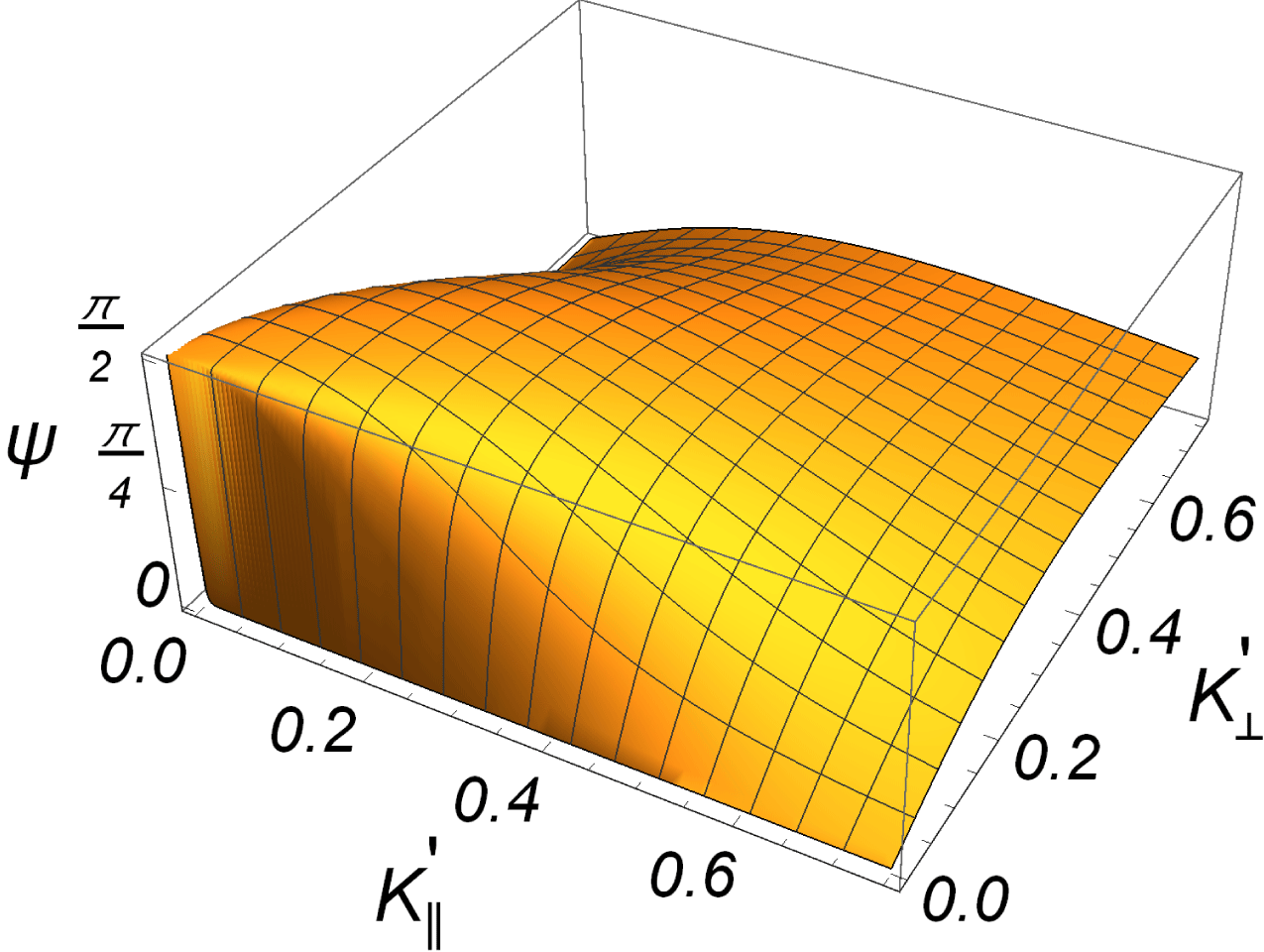The real part of the frequency will be $\boldsymbol{u}_{g}\boldsymbol{\cdot }\boldsymbol{K}^{\prime }$ to lowest approximation. In figure 11 we show for reference the angle $\unicode[STIX]{x1D713}$ between $\boldsymbol{K}_{0}^{\prime }$ and the group velocity $\boldsymbol{u}_{g}^{\prime }(\boldsymbol{K}^{\prime })\equiv \unicode[STIX]{x1D735}_{\boldsymbol{K}^{\prime }}\unicode[STIX]{x1D6FA}^{\prime }(\boldsymbol{K}^{\prime })$ .

Figure 11.

Angle $\unicode[STIX]{x1D713}$ between the group velocity $\boldsymbol{u}_{g}^{\prime }(\boldsymbol{K}^{\prime })\equiv \unicode[STIX]{x1D735}_{\boldsymbol{K}^{\prime }}\unicode[STIX]{x1D6FA}^{\prime }(\boldsymbol{K}^{\prime })$ and the wave vector $\boldsymbol{K}^{\prime }$ for the electron plasma waves, shown here for the case where $\unicode[STIX]{x1D701}=1$ . A singularity at $\boldsymbol{K}^{\prime }=\{0,0,0\}$ is caused by the omission of an electromagnetic component.

4.4 Two waves

As the first step towards a spectrum of waves we can consider a superposition of two plane electron plasma waves. Two counter-propagating electron plasma waves have been studied analytically (Pavlenko & Petviashvili Reference Pavlenko and Petviashvili1977) as well as experimentally (Wong & Quon Reference Wong and Quon1975; Michelsen et al. Reference Michelsen, Pécseli, Rasmussen and Sato1977; Leung, Tran & Wong Reference Leung, Tran and Wong1982), so we choose this particular example.

Figure 12.

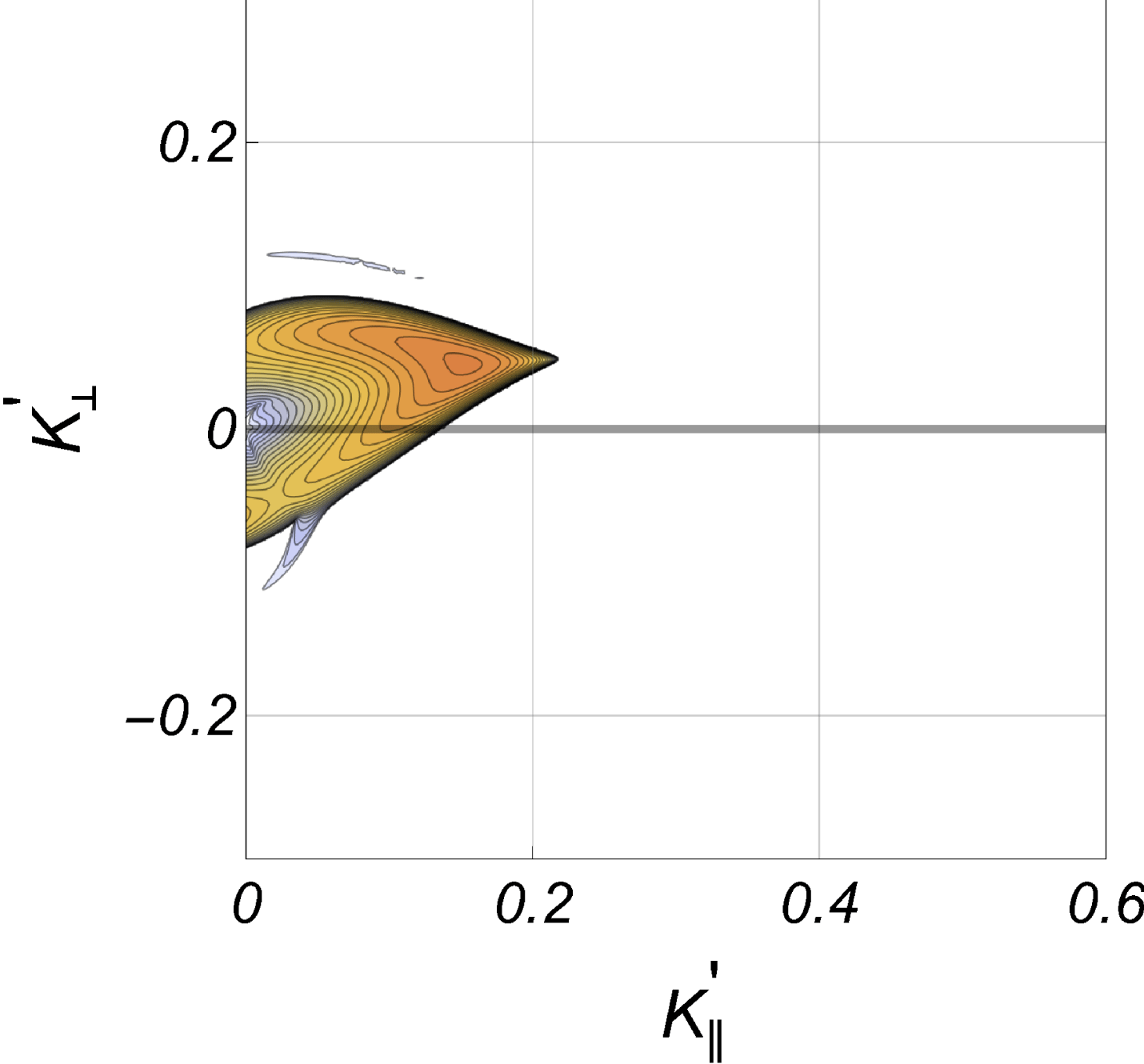
$\text{Im}\{\unicode[STIX]{x1D6FA}^{\prime }\}$ for a reference plane wave with $\boldsymbol{K}_{0}^{\prime }=\{0.25,0,0.05\}$ and $A_{0}^{2}=0.5$ . A small wavenumber component $\bot \boldsymbol{B}_{0}$ is included to break the symmetry. The maximum contour level is at 0.025. For these parameters we can have no decay to the high-frequency ion branch, and the growth rates shown are for the modulational instability, as confirmed also by (4.11).

Figure 13.

$\text{Im}\{\unicode[STIX]{x1D6FA}^{\prime }\}$ for two counter-propagating plane waves with $\boldsymbol{K}_{0}^{\prime }=\pm \{0.25,0,0.05\}$ and equal amplitudes $A_{0}^{2}=0.5$ . Superimposed on the figure we have the contour corresponding to the decay into $\unicode[STIX]{x1D6FA}_{L-}^{\prime }(\boldsymbol{K}^{\prime })$ in (4.6), as in e.g. figures 3 and 4. See figure 12 for the characteristics of one of the waves entering the construction for the present figure: the colour coding is the same for these two figures. The present figure is symmetric with respect to the origin.

In nature, and the Earth’s ionosphere in particular, we are most likely to find $\boldsymbol{K}_{0}^{\prime }$ nearly parallel to $\boldsymbol{B}_{0}$ since electron waves are there excited most easily by low density magnetic field aligned electron beams (Guio & Forme Reference Guio and Forme2006) propagating along $\boldsymbol{B}_{0}$ . In figure 12 taken together with figure 13 we show a generalization of the single wave case where now the modulational instability dominates. The decay to the high-frequency branch $\unicode[STIX]{x1D6FA}_{L+}^{\prime }(\boldsymbol{K}^{\prime })$ is not accessible for the present parameters, and figure 12 for the reference plane wave accounts for the modulational instability only. When we have two waves with twice the net wave energy density, see figure 13, we find a slight modification of the growth rate of the modulational instability as compared to the single mode case. More importantly we observe decay to the low-frequency branch $\unicode[STIX]{x1D6FA}_{L-}^{\prime }(\boldsymbol{K}^{\prime })$ in (4.6), which has otherwise not been found in any calculation for a single plane wave. The figure changes if we ignore the magnetic field in the description of the low-frequency ion dynamics. Although it might be tempting to ignore the terms containing $m/M$ due to the smallness of the electron–ion mass ratio, we find that for spectra deviating from a single plane wave, this ‘near-zero-frequency’ branch can nonetheless have importance for the nonlinear electron waves in even weakly magnetized plasmas. For most relevant decay products we have wave vectors $K>\unicode[STIX]{x1D6FA}_{\text{ci}}/C_{s}$ , implying that the phase velocities associated with this branch are much smaller than $C_{s}$ . In the following this will be referred to as ‘the slow mode’. For the relevant particular case with $K\sim \sqrt{m/M}/\unicode[STIX]{x1D706}_{\text{De}}$ we find a characteristic velocity for the slow mode to be ${\sim}C_{s}(\unicode[STIX]{x1D714}_{\text{ce}}/\unicode[STIX]{x1D714}_{\text{pe}})\ll C_{s}$ for our conditions. Incidentally, we note faint signs of this slow mode being excited already in figure 12, near $K_{\bot }^{\prime }\approx 0.1$

Figure 14.

$\text{Im}\{\unicode[STIX]{x1D6FA}^{\prime }\}$ for two counter-propagating plane waves with $\boldsymbol{K}_{0}^{\prime }=\{\pm 0.25,0,0.05\}$ and equal amplitudes $A_{0}^{2}=0.5$ . The maximum contour level is at 0.03. See again figure 12 for the characteristics of one of the waves entering the construction for the present figure. From $\text{Re}\{\unicode[STIX]{x1D6FA}^{\prime }\}$ we find that in the present case the waves are propagating, i.e. they do not correspond to the quasi-stationary mode. The symmetry axis is horizontal at $K_{\bot }^{\prime }=0$ in this figure.

When interpreting figure 13 we bear in mind that implicit in the derivation is that the phases of the two waves are random and independent, as implied in what is often termed the ‘random phase approximation’ (Nicholson Reference Nicholson1983; Pécseli Reference Pécseli2014, Reference Pécseli2016). Physically, this can be realized by reflection of a plane wave from a slowly moving or oscillating reflector (Dysthe, Pécseli & Trulsen Reference Dysthe, Pécseli and Trulsen1983).

An interesting interpretation of the slow mode relates to observations of naturally enhanced ion acoustic lines (NEIALs). Here non-thermal asymmetric up and down propagating sound waves are observed, but in addition also an enhanced or anomalous level of slow or stationary plasma density variations are found (Rietveld, Collis & St-Maurice Reference Rietveld, Collis and St-Maurice1991; Buchert et al. Reference Buchert, van Eyken, Ogawa and Watanabe1999; Sedgemore-Schulthess & St-Maurice Reference Sedgemore-Schulthess and St-Maurice2001). An interpretation in terms of strongly nonlinear Langmuir waves has been suggested (Guio & Forme Reference Guio and Forme2006; Isham et al. Reference Isham, Rietveld, Guio, Forme, Grydeland and Mjølhus2012), where localized quasi-stationary wave filled cavities develop. Our results indicate that slow or stationary plasma density variations can be found for weakly magnetized plasmas even for weakly nonlinear electron plasma waves, without cavity formation.

We point out, however, that the slow mode is not excited in all multi-wave cases. We show as an example two obliquely propagating waves with $\boldsymbol{K}_{0}^{\prime }=\{\pm 0.05,0,0.25\}$ in figure 14. We find that the decay waves are propagating here. The growth rate of the modulational instability found for one of the plane wave components is on the other hand strongly modified in this case. The results in figure 13 refer to a near ‘head on’ reflection of a wave, while figure 14 corresponds to oblique reflection, reminiscent of, for instance, Lloyd’s single mirror experiment.

4.5 Four waves

With some imposed symmetry conditions it is possible to solve the basic equation also for more than 2 wave modes. As an illustration we show here results for the case where 4 waves are excited with equal amplitudes, where $\boldsymbol{K}_{0}^{\prime }=\{\pm 0.05,0,\pm 0.25\}$ , see figure 15. The maximum growth rate is decreased in comparison to the one found for the 2 wave mode case illustrated in figures 13 and 14 which involves the same magnitude of the wavenumber components. Also in figure 15 we find the slow mode to be excited.

Figure 15.

Average $\text{Im}\{\unicode[STIX]{x1D6FA}^{\prime }\}$ for the case where 4 plane waves are excited with $\boldsymbol{K}_{0}^{\prime }=\{\pm 0.25,0,\pm 0.05\}$ and equal amplitudes $A_{0}^{2}=0.25$ . The maximum contour level is 0.015. The full figure is symmetric with respect to both the vertical and horizontal axes.

As expected, we find that the increased number of wave modes gives rise to an increasing complexity of the dispersion relation. The most conspicuous new feature of the four wave case is however the excitation of two dispersion relation branches to reach substantial growth rates. The imaginary part of the average of these two branches is shown in figure 15. Also in this case we find excitation of the ‘slow mode’, substantiating the claim that this mode is generated by distributions of wave modes over a substantial region of the wavenumber space, when the average of the wave vectors is at or near the origin $\boldsymbol{K}_{0}^{\prime }=\{0,0,0\}$ . A general plausible conclusion from the limited number of cases studied here is that the number of low-frequency modes being excited is increased for increasing number of high frequency modes, covering a wide range in $\boldsymbol{K}_{0}^{\prime }$ space. Also the maximum growth rate is decreasing and, as mentioned, we find a possibility for exciting slow modes. These observations were also confirmed by considering a three wave case.

The many mode case has several similarities with the Vlasov equation describing collisionless plasmas. The one mode case corresponds to a single cold beam in such a kinetic model. Addition of many plane waves corresponds to increasing the number of cold beams in the Vlasov model (Marcuvitz Reference Marcuvitz1980; Kontar Reference Kontar2001). Indeed, this similarity has been pursued with some success in numerical simulations (Tappert & Cole Reference Tappert and Cole1971; Pécseli & Trulsen Reference Pécseli and Trulsen1990, Reference Pécseli and Trulsen1992), although seemingly only in a one-dimensional case so far. The analogy with the Vlasov equation is only complete if we ignore the dispersion of the propagating wave packets, i.e. wave packets are only analogous to particles when their dispersion is ignored. This feature is included in the present analysis, as already mentioned, so the present results are more general than those derived from the standard wave kinetic equation (Camac et al. Reference Camac, Kantrowitz, Litvak, Patrick and Petschek1962; Kadomtsev Reference Kadomtsev1965; Vedenov, Gordeev & Rudakov Reference Vedenov, Gordeev and Rudakov1967; Shukla & Farid Reference Shukla and Farid1999). An often used argument for the validity of these quasi-particle models is that for wide band spectra the dispersion of a spatially localized wave field due to distributed group velocities is dominating the dispersion due to what is determined by the curvature of the dispersion relation. It should be noted however that a correct account for this latter dispersion introduces a characteristic length scale particularly relevant for modulational instabilities (Pécseli Reference Pécseli2014; Kono & Pécseli Reference Kono and Pécseli2016). This length scale is not present in the quasi-particle model.

5.1 Decay instability

We here show illustrative results for the case with a ‘cigar’ or ‘needle’ shaped decaying spectra, centred at some $\boldsymbol{K}_{0}^{\prime }$ defining the average wavenumber of propagation, in the present case along $\boldsymbol{B}_{0}$ . This condition is relevant for electron waves excited by magnetic field aligned electron beams with a large velocity spread. The wave spectrum is one-dimensional but the decay products have distributed directions, so the problem as such is fully three-dimensional. The model is restrictive, but relevant nonetheless for realistic conditions. The single mode, plane wave, case is similar to the one illustrated in figure 7, but for the present problem with $K_{\bot }^{\prime }=0$ being the symmetry axis. The wave spectrum is widened along $\boldsymbol{B}_{0}$ by increasing $\unicode[STIX]{x1D6E5}_{\Vert }^{\prime }$ , keeping $\unicode[STIX]{x1D6E5}_{\bot }^{\prime }=0$ . Results are shown in figures 16 and 17. In particular in figure 17 it is understood that we have $\unicode[STIX]{x1D6E5}^{\prime }\rightarrow \unicode[STIX]{x1D6E5}_{\Vert }^{\prime }$ for the curve given by the full line, while $\unicode[STIX]{x1D6E5}^{\prime }\rightarrow \unicode[STIX]{x1D6E5}_{\bot }^{\prime }$ for the dashed line. We have in all cases $\int \text{d}\boldsymbol{K}^{\prime }G(\boldsymbol{K}^{\prime })=\text{const.}$ while $\unicode[STIX]{x1D6E5}^{\prime }$ varies. Wider spectra give reduced $\text{Im}\{\unicode[STIX]{x1D6FA}^{\prime }\}$ and wider decay ranges as evidenced by the $K_{\bot }^{\prime }$ -variation of $\text{Im}\{\unicode[STIX]{x1D6FA}^{\prime }\}$ . The stabilizing effect of the spectral broadening is evident. The effect is most pronounced for small spectral power densities.

In figure 17 we included with dashed lines the results for the case where $\boldsymbol{K}_{0}^{\prime }\bot \boldsymbol{B}_{0}$ and the spectrum is widened along the direction $\bot \boldsymbol{B}_{0}$ , i.e. along the $x$ -axis. The main features of the results are the same in all of the cases shown, apart from some changes in numerical factors. All curves shown in figure 17 will depend on the sampling wavenumbers. The main characteristics are the same in all cases, although waves with a dominant direction of propagation $\bot \boldsymbol{B}_{0}$ appear less sensitive to spectral broadening than those propagating along $\boldsymbol{B}_{0}$ . For the range of the spectra considered here we do not find the excitation of the ‘slow mode’ low-frequency waves seen in figure 13. Since the wave spectrum has an average propagation along $\boldsymbol{B}_{0}$ , excitation of the slow wave mode is not to be expected here.

5.2 Modulational instability

We studied the effect of varying $\unicode[STIX]{x1D6E5}_{\Vert }^{\prime }$ on $\text{Im}\{\unicode[STIX]{x1D6FA}^{\prime }\}$ also for the modulational instability. The results are shown in figure 18. The plane wave, single mode, equivalent of this case is similar to that shown in figure 12 except with $K_{\bot }^{\prime }=0$ being the symmetry axis. The wave spectrum is also here needle or cigar shaped along $\boldsymbol{B}_{0}$ and narrow in the direction $\bot \boldsymbol{B}_{0}$ .

Figure 18.

Variation of the growth rate for the modulational instability for varying $\unicode[STIX]{x1D6E5}_{\Vert }^{\prime }$ . We have $A_{0}^{2}=0.4$ , $K_{0\Vert }^{\prime }=0.25$ , and $\unicode[STIX]{x1D6E5}_{\Vert }^{\prime }=0.01,0.02,0.05,0.1$ and $0.2$ . The variation of the maximum value of $\text{Im}\{\unicode[STIX]{x1D6FA}^{\prime }\}$ is sampled at $K_{\Vert }^{\prime }=0.1$ . The results apply for the uncompensated case with $\int \text{d}\boldsymbol{K}^{\prime }G(\boldsymbol{K}^{\prime })=\text{const}$ .

The results if figure 18 assume $\int \text{d}\boldsymbol{K}^{\prime }G(\boldsymbol{K}^{\prime })=\text{const}$ . The wave energy density is thus not kept constant for this case. To illustrate the difference between this and the energy density conserving case we show in figure 19 the corresponding results when the electric field power density $\int \text{d}\boldsymbol{K}^{\prime }K^{\prime 2}G(\boldsymbol{K}^{\prime })=\text{const}$ . The two results are nearly identical for small $\unicode[STIX]{x1D6E5}^{\prime }$ . More generally, we find here that an increasing spectral width gives rise to a steadily decreasing growth rate of the modulational instability, best seen at $K_{\bot }^{\prime }\approx 0$ . The increase in bandwidth is nearly the same for figure 18 and for figure 19, at least for the $\unicode[STIX]{x1D6E5}^{\prime }$ interval shown.

Figure 19.

Illustration of the compensated case where $\int \text{d}\boldsymbol{K}^{\prime }K^{\prime 2}G(\boldsymbol{K}^{\prime })=\text{const.}$ , showing the variation of the growth rate for the modulational instability for varying $\unicode[STIX]{x1D6E5}_{\Vert }^{\prime }$ . As in figure 18, we have $A_{0}^{2}=0.4$ , $K_{0\Vert }^{\prime }=0.25$ and $\unicode[STIX]{x1D6E5}_{\Vert }^{\prime }=0.01,0.02,0.05,0.1$ and $0.2$ . The variation of the maximum value of $\text{Im}\{\unicode[STIX]{x1D6FA}^{\prime }\}$ is sampled at $K_{\Vert }^{\prime }=0.1$ .

The variation of $\text{Im}\{\unicode[STIX]{x1D6FA}^{\prime }\}$ with varying spectral width $\unicode[STIX]{x1D6E5}_{\Vert }^{\prime }$ for given $\boldsymbol{K}_{0}^{\prime }$ depends in general on $\boldsymbol{K}^{\prime }$ . For the modulational instability, in the present case with a magnetic field aligned ‘cigar-like’ spectrum, the dependence is weakest for the filamentation instability where $\boldsymbol{K}^{\prime }\bot \boldsymbol{K}_{0}^{\prime }$ .