2.1 Cell-free layer calculation

A fundamental component to the present analysis is the means by which the CFL is determined. The methodologies used to determine the CFL in previous experimental works have typically involved constructing some form of an RBC core used in conjunction with the location of the vessel walls. Among these works, however, different approaches have been taken. Earlier in vivo works (e.g. Bloch Reference Bloch1962; Tateishi et al. Reference Tateishi, Suzuki, Soutani and Maeda1994; Soutani et al. Reference Soutani, Suzuki, Tateishi and Maeda1995; Maeda et al. Reference Maeda, Suzuki, Tanaka and Tateishi1996) and in vitro works (e.g. Bugliarello & Sevilla Reference Bugliarello and Sevilla1970; Reinke et al. Reference Reinke, Gaehtgens and Johnson1987) determined the CFL thickness by visual observation and analysis of video images. More recently, in vivo works such as Kim et al. (Reference Kim, Kong, Popel, Intaglietta and Johnson2006) or Ong et al. (Reference Ong, Jain, Namgung, Woo, Sakai, Lim, Chun and Kim2011) have developed automated image analysis methods to digitally construct the RBC core and cell-free regions at individual instants in time. Specifically, the method developed in Kim et al. (Reference Kim, Kong, Popel, Intaglietta and Johnson2006) constructed the core and cell-free regions as a binary image which assumed a continuous core between any plasma gaps separating individual RBCs along the length. Ong et al. (Reference Ong, Jain, Namgung, Woo, Sakai, Lim, Chun and Kim2011) improved on this with a greyscale image-based method that provides increased accuracy in faint areas.

Somewhat similar approaches have been adopted in previous computational modelling. Fedosov et al. (Reference Fedosov, Caswell, Popel and Karniadakis2010) simulated RBCs flowing in a straight tube using a dissipative particle dynamics method, and constructed an RBC core by projecting the cell outline along the vessel length onto a 2D plane in a manner similar to Kim et al. (Reference Kim, Kong, Popel, Intaglietta and Johnson2006). Yin & Zhang (Reference Yin and Zhang2012), for their 2D lattice-Boltzmann simulations, determined the CFL as the average of the closest cell-wall distances between each side of the vessel. For the simulations in Yin et al. (Reference Yin, Thomas and Zhang2013), the CFL thickness was determined as the boundary of the region near the wall that is occupied by 2.5 % of the total RBC volume, while Ye et al. (Reference Ye, Ju and Kim2016) used an occurrence frequency distribution of CFL values at locations in the modelled vessel.

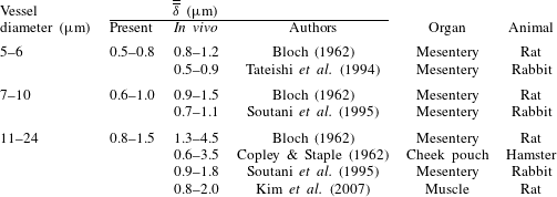
Evidently, a wide variety of approaches have been used to determine the CFL in prior works. In the present work, because of the geometric complexity of the microvascular networks, and the resulting effect on the formation of the RBC core, a 2D projection of the core to determine the CFL would not be sufficient. Furthermore, the distribution of the RBCs across a network is highly heterogeneous, and constantly changes over time. As such, the CFL distribution across the network is heterogeneous and time-dependent. Owing to the heterogeneity of the RBC distribution, some vessels are constantly filled with cells, while some have intermittent flows of cells. In many vessels, especially in the small capillaries, there are instants when only one or two cells are flowing through a vessel, or cells flow through a vessel in a manner in which there are plasma gaps in between the cells along the vessel length. A methodology is thus needed for the present work to accurately compute the 3D time-dependent CFL under these different flow conditions. As such, the procedure developed for calculation of the CFL in the present work is given in appendix A. Also included is a comparison with in vivo values from the literature.

3.1 Three-dimensionality of cell-free layer

We first describe the general 3D nature of the CFL as predicted in the simulated networks. The analysis of the underlying mechanisms is presented in the subsequent sections.

Figure 2.

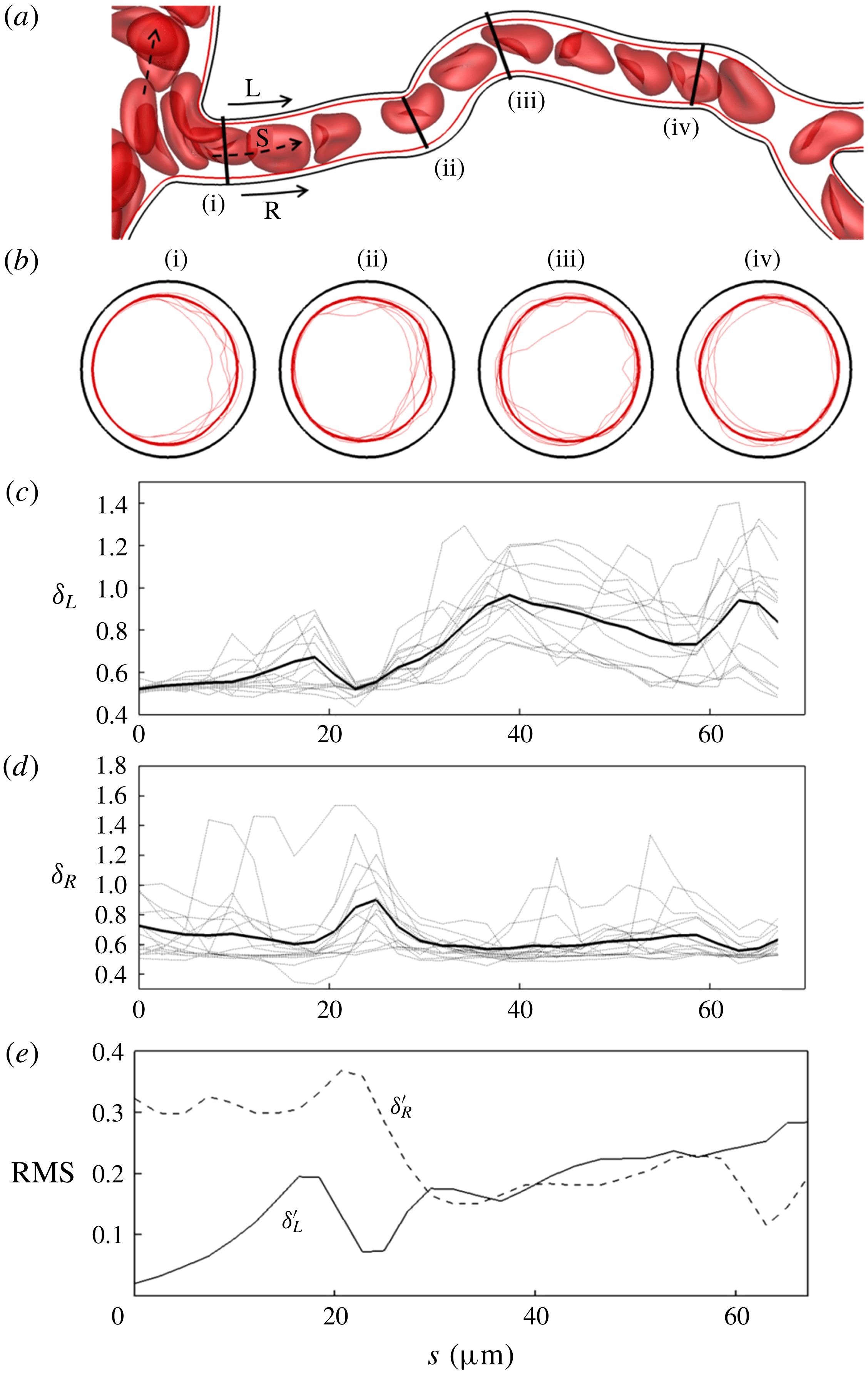
(a) An instant of RBCs flowing in an example vessel in one of the simulated networks. Here R and L denote the right and left sides in the plane of the figure, respectively. (b) The time-averaged (thick line) and instantaneous (thin lines; several instants are shown) RBC core over the vessel cross-section at four different axial locations. (c,d) Time-averaged (thick line) and instantaneous (thin lines) CFL thickness along L and R, respectively. (e) Root mean square (r.m.s.) of temporal fluctuations in the CFL thickness along L and R.

The three-dimensionality is first described using a representative vessel as shown in figure 2(a). The time-dependent profiles of the RBC core over the vessel cross-sections are shown in figure 2(b) at four different locations along the vessel length, along with the time-averaged profiles superimposed. As figure 2(b) suggests, the time-dependent profiles at any cross-section are highly non-circular, significantly distinct at each instant, and deviate significantly from the time-averaged profiles. Also, at any time instant the cross-sectional profiles are different at different locations. To further demonstrate the 3D and non-circular nature of the CFL, we consider its variation along the vessel length but at two diametrically opposite sides, L and R, as shown in figure 2(a). The CFL thicknesses along these sides are denoted as $\unicode[STIX]{x1D6FF}_{L}(s,t)$ and $\unicode[STIX]{x1D6FF}_{R}(s,t)$ , respectively, and both time-dependent and time-averaged results are presented in figure 2(c,d). While these quantities themselves give the thickness as in a 2D projection approach, when taken in conjunction with the cross-sectional profiles these collectively paint a 3D picture of the CFL. Figure 2(b–d) shows that both the time-dependent and time-averaged CFL vary significantly along the vessel length. The differences between $\unicode[STIX]{x1D6FF}_{L}$ and $\unicode[STIX]{x1D6FF}_{R}$ are significant, for both the time-dependent and time-averaged results, serving as evidence of the asymmetric nature of the CFL. While both time-averaged $\unicode[STIX]{x1D6FF}_{L}$ and $\unicode[STIX]{x1D6FF}_{R}$ vary along the length, $\unicode[STIX]{x1D6FF}_{L}$ shows a greater variation than $\unicode[STIX]{x1D6FF}_{R}$ . Furthermore, $\unicode[STIX]{x1D6FF}_{L}$ generally increases along the vessel length while $\unicode[STIX]{x1D6FF}_{R}$ does not have a net change between the vessel entrance and exit. The root mean square (r.m.s.) values of the temporal fluctuations of $\unicode[STIX]{x1D6FF}_{L}$ and $\unicode[STIX]{x1D6FF}_{R}$ scaled by the time-averaged thickness at each location along the length are shown in figure 2(e). Interestingly, temporal fluctuations in $\unicode[STIX]{x1D6FF}_{L}$ generally increase along the vessel length, while those in $\unicode[STIX]{x1D6FF}_{R}$ decrease.

Figure 2 generally shows that not only is the time-dependent CFL highly 3D and asymmetric, but the time-averaged CFL is as well. In contrast, for a fully developed flow in straight tubes of circular cross-section, though the time-dependent CFL is generally 3D, the time-averaged CFL is axisymmetric. Thus in the present work we primarily focus on studying the three-dimensionality in the time-averaged CFL as it arises in complex networks.

To quantify the 3D and asymmetric nature of the time-averaged CFL, first we consider an asymmetry parameter defined as

(3.1) $$\begin{eqnarray}\unicode[STIX]{x1D700}(s)=\frac{\overline{\unicode[STIX]{x1D6FF}}_{max}(s)}{\overline{\unicode[STIX]{x1D6FF}}_{min}(s)},\end{eqnarray}$$

where $\overline{\unicode[STIX]{x1D6FF}}_{max}(s)$ and $\overline{\unicode[STIX]{x1D6FF}}_{min}(s)$ are the maximum and minimum values, respectively, of the time-averaged CFL thickness over the vessel cross-section $(0\leqslant \unicode[STIX]{x1D703}<2\unicode[STIX]{x03C0})$ at any location $s$ along the vessel length. This gives a value of one for a symmetric profile, and values greater than one for increasing asymmetry. The $\unicode[STIX]{x1D700}(s)$ value is plotted in figure 3(a) for a few representative vessels with length-to-diameter ratio in the range of 10–15. Several important observations are made here. First, this shows that, even for relatively long vessels, the time-averaged CFL does not become axisymmetric over the length. While for some vessels the profile becomes more symmetric near the end, for others it becomes more asymmetric. Second, while there may be a net increase or decrease in $\unicode[STIX]{x1D700}$ between the inlet and exit of a vessel, there is a significant fluctuation along the vessel length. This often results in the extremum of $\unicode[STIX]{x1D700}$ occurring at locations in the middle of the vessels rather than at the inlet and exit. In vessels where the extremum of $\unicode[STIX]{x1D700}$ does occur at the inlet and outlet, $\unicode[STIX]{x1D700}$ does not typically change monotonically along the length but rather fluctuates significantly as well. Even when $\unicode[STIX]{x1D700}$ is nearly the same at the inlet and outlet, in between, fluctuations of large magnitudes are observed. These results are in contrast to what would happen in a straight tube, where any CFL asymmetry at the inlet would monotonically decrease over the vessel length.

Figure 3.

(a) The CFL asymmetry parameter $\unicode[STIX]{x1D700}$ along the length for several representative vessels in the network. (b) The change in asymmetry, $\unicode[STIX]{x1D700}|_{s=L}-\unicode[STIX]{x1D700}|_{s=0}$ , between vessel inlet and outlet versus the cumulative change $\unicode[STIX]{x0394}\unicode[STIX]{x1D700}$ over the entire length, for all vessels (data points). The straight lines correspond to a monotonic change in $\unicode[STIX]{x1D700}$ over the length.

To quantify the CFL asymmetry $\unicode[STIX]{x1D700}$ for all vessels in the network, we compute the difference between $\unicode[STIX]{x1D700}$ at the beginning and end of each vessel, i.e.  $\unicode[STIX]{x1D700}|_{s=L}-\unicode[STIX]{x1D700}|_{s=0}$ , and plot this with respect to the cumulative change in $\unicode[STIX]{x1D700}$ over the length defined as $\unicode[STIX]{x0394}\unicode[STIX]{x1D700}=\sum _{i}|\text{d}\unicode[STIX]{x1D700}(s_{i})|$ . Here, $\unicode[STIX]{x0394}\unicode[STIX]{x1D700}$ is evaluated by dividing each vessel into $N$ finite segments, each given by the index $i$ . The relationship between these quantities is presented in figure 3(b). If $\unicode[STIX]{x1D700}$ were to change monotonically over the length, then $\unicode[STIX]{x0394}\unicode[STIX]{x1D700}$ would equal the magnitude of $\unicode[STIX]{x1D700}|_{s=L}-\unicode[STIX]{x1D700}|_{s=0}$ . This relationship is given by two straight lines in figure 3(b): the line $\unicode[STIX]{x0394}\unicode[STIX]{x1D700}=-(\unicode[STIX]{x1D700}|_{s=L}-\unicode[STIX]{x1D700}|_{s=0})$ corresponds to a straight tube, where an asymmetric CFL profile at the vessel entrance monotonically shifts towards a symmetric one with increasing axial distance. In contrast, the line $\unicode[STIX]{x0394}\unicode[STIX]{x1D700}=+(\unicode[STIX]{x1D700}|_{s=L}-\unicode[STIX]{x1D700}|_{s=0})$ means the asymmetry at the inlet monotonically increases along the length. As figure 3(b) shows, most data points from the simulations lie above the lines, i.e.  $\unicode[STIX]{x0394}\unicode[STIX]{x1D700}>|(\unicode[STIX]{x1D700}|_{s=L}-\unicode[STIX]{x1D700}|_{s=0})|$ , meaning that the CFL does not change monotonically along the vessel length. Even for vessels in which $\unicode[STIX]{x1D700}|_{s=L}-\unicode[STIX]{x1D700}|_{s=0}\approx 0$ , $\unicode[STIX]{x0394}\unicode[STIX]{x1D700}$ may have large values. Furthermore, of the points that do nearly fall on the lines, some of them are on the $\unicode[STIX]{x0394}\unicode[STIX]{x1D700}=+(\unicode[STIX]{x1D700}|_{s=L}-\unicode[STIX]{x1D700}|_{s=0})$ line, which means the asymmetry at the inlet monotonically increases with length. Overall, figure 3(b) suggests that, while there may be a net increase or decrease in $\unicode[STIX]{x1D700}$ between the inlet and outlet, the evolution of $\unicode[STIX]{x1D700}$ over the length is much more complex, and, in most vessels, the time-averaged CFL profile varies significantly and non-monotonically along the vessel length.

Figure 4.

Axial variation of the angular locations on the vessel cross-section where the maximum and minimum time-averaged CFL thicknesses occur, denoted by the angles $\unicode[STIX]{x1D703}_{\unicode[STIX]{x1D6FF}=\unicode[STIX]{x1D6FF}\,max}$ and $\unicode[STIX]{x1D703}_{\unicode[STIX]{x1D6FF}=\unicode[STIX]{x1D6FF}\,min}$ , respectively. Results are shown for the same six vessels as in figure 3(a), with angles given as fractions of  $\unicode[STIX]{x03C0}$ .

The number of segments $N$ used in the above analysis typically corresponded to a spacing of roughly one-quarter of the vessel diameter. This was found to be fine enough to capture variations of the RBC core along vessel lengths, and resolve the curvature of the vessel centreline. Since these variations are adequately captured, the resolution is deemed sufficient.

Additional quantification of the 3D, non-symmetric nature of the time-averaged CFL is made by considering the angular locations on the vessel cross-section where the maximum and minimum thickness values occur, denoted by the angles $\unicode[STIX]{x1D703}_{\unicode[STIX]{x1D6FF}=\unicode[STIX]{x1D6FF}\,max}$ and $\unicode[STIX]{x1D703}_{\unicode[STIX]{x1D6FF}=\unicode[STIX]{x1D6FF}\,min}$ , respectively. As noted in appendix A, $\unicode[STIX]{x1D703}$ is defined using the vessel centreline as the origin and looking downstream in the flow direction. Here, $\unicode[STIX]{x1D703}=0$ is located on the plane passing through the vessel centreline at the location on the perimeter closest to the upstream bifurcation (see figure 21 in appendix A). Figure 4 presents the variations in $\unicode[STIX]{x1D703}_{\unicode[STIX]{x1D6FF}=\unicode[STIX]{x1D6FF}\,max}$ and $\unicode[STIX]{x1D703}_{\unicode[STIX]{x1D6FF}=\unicode[STIX]{x1D6FF}\,min}$ over the length of the same representative vessels as considered in figure 3(a). When plotting these values along the vessel length, the sign of $\unicode[STIX]{x1D703}$ was chosen so as to result in a smooth curve without discontinuities. Figure 4 shows that there are significant variations in $\unicode[STIX]{x1D703}_{\unicode[STIX]{x1D6FF}=\unicode[STIX]{x1D6FF}\,max}$ and $\unicode[STIX]{x1D703}_{\unicode[STIX]{x1D6FF}=\unicode[STIX]{x1D6FF}\,min}$ along the vessel length. Another interesting observation in figure 4 is that $\unicode[STIX]{x1D703}_{\unicode[STIX]{x1D6FF}=\unicode[STIX]{x1D6FF}\,min}\approx 0$ at vessel entrances, meaning that the location of the minimum CFL thickness occurs on the side of the vessel that is closest to the upstream bifurcation. In contrast, $\unicode[STIX]{x1D703}_{\unicode[STIX]{x1D6FF}=\unicode[STIX]{x1D6FF}\,max}$ at vessel entrances is such that the maximum thickness is observed to occur at any location over the perimeter. Additional analysis of $\unicode[STIX]{x1D703}_{\unicode[STIX]{x1D6FF}=\unicode[STIX]{x1D6FF}\,max}$ and $\unicode[STIX]{x1D703}_{\unicode[STIX]{x1D6FF}=\unicode[STIX]{x1D6FF}\,min}$ and the underlying cellular-scale mechanisms will be considered in later sections. It is noted that, while these examples utilize vessels on the arterial side, similar fluctuations and variations with vessel length were observed in post-capillary venules as well.

Together, figures 2–4 demonstrate the highly complex, 3D and asymmetric nature of the time-averaged CFL in the vessels comprising the network. Next, we identify and analyse the mechanisms that give rise to such complexity. These mechanisms are discussed as they arise in three different facets of the networks, namely, along the vessel lengths, and over the bifurcations and the mergers.

3.2 Mechanism causing cell-free layer variations along vessel length

In this section, we identify a primary mechanism causing the axial variations in the time-averaged CFL. In general, the CFL at the entrance to a vessel in the networks is asymmetric due to the presence of the upstream bifurcation or merger. If the vessel were straight, the asymmetric CFL at the entrance would gradually shift towards a symmetric profile with increasing axial distance. This has been shown in vivo in such works as Ong et al. (Reference Ong, Jain and Kim2012), and in silico in Katanov et al. (Reference Katanov, Gompper and Fedosov2015), among others. Most vessels in the networks are, however, winding. We find that vessel tortuosity results in the increased asymmetry of the CFL along the length, as discussed below.

To quantify the effect of vessel tortuosity, we consider the curvature of the vessel centreline, defined as $\unicode[STIX]{x1D705}(s)=R/r(s)$ , where $r(s)$ is the radius of curvature of the vessel centreline at an axial location $s$ , and $R$ is the vessel radius. As a measure of tortuosity, the mean absolute curvature is defined as

(3.2) $$\begin{eqnarray}\overline{\unicode[STIX]{x1D705}}=\frac{\displaystyle \mathop{\sum }_{i=1}^{N}|\unicode[STIX]{x1D705}(s_{i})|}{N},\end{eqnarray}$$

which is computed by dividing each vessel into $N$ finite segments, as previously described. In addition, as a measure of the axial variation of the CFL, we define the mean absolute change in the asymmetry parameter $\unicode[STIX]{x1D700}$ as

(3.3) $$\begin{eqnarray}\overline{\unicode[STIX]{x0394}\unicode[STIX]{x1D700}}=\frac{\displaystyle \mathop{\sum }_{i=1}^{N}|\text{d}\unicode[STIX]{x1D700}(s_{i})|}{N}.\end{eqnarray}$$

In figure 5, we plot $\overline{\unicode[STIX]{x0394}\unicode[STIX]{x1D700}}$ as a function of $\overline{\unicode[STIX]{x1D705}}$ for all vessels. This figure shows that $\overline{\unicode[STIX]{x0394}\unicode[STIX]{x1D700}}$ generally increases with increasing $\overline{\unicode[STIX]{x1D705}}$ , which implies that the CFL asymmetry is higher in winding vessels. The plot, however, also shows a noticeable scatter, which will be discussed later.

Figure 5.

Effect of vessel tortuosity. The mean absolute change in asymmetry, $\overline{\unicode[STIX]{x0394}\unicode[STIX]{x1D700}}$ , is presented as a function of the mean absolute curvature, $\overline{\unicode[STIX]{x1D705}}$ , for every vessel. The red dashed line is a linear regression of the data.

It is noted that $\unicode[STIX]{x0394}\unicode[STIX]{x1D700}$ is the change in CFL asymmetry, not the asymmetry itself. The trend that $\unicode[STIX]{x0394}\unicode[STIX]{x1D700}\rightarrow$ 0 as $\unicode[STIX]{x1D705}\rightarrow 0$ as in figure 5 means that, for a relatively straight vessel, the change in the CFL asymmetry over the vessel length tends to be very small. This is expected, for example, because the CFL profile can be asymmetric at the inlet to a vessel, but if the vessel has a small curvature the change in the CFL asymmetry will be small.

Figure 6.

Effect of vessel centreline curvature on the time-averaged CFL profile. (a) A representative vessel showing the time-averaged RBC core and the cross-sectional profiles at four axial locations marked as (i)–(iv). Here $\overline{\unicode[STIX]{x1D6FF}_{L}}(s)$ and $\overline{\unicode[STIX]{x1D6FF}_{R}}(s)$ are the CFL thicknesses along the left and right sides of the vessel, respectively, in the plane of the figure looking in the flow direction (arrow). (b) Plots of $\overline{\unicode[STIX]{x1D6FF}_{L}}/\overline{\unicode[STIX]{x1D6FF}_{R}}$ (dashed line, left axis) and centreline curvature $\unicode[STIX]{x1D705}$ (solid line, right axis) along the vessel length.

Having established that the CFL asymmetry generally increases with increasing vessel tortuosity, we now consider how the CFL profile at an axial location is affected by the centreline curvature at that location. This is illustrated in figure 6 using a representative vessel from one network. The time-averaged RBC core along the vessel length is shown, along with the cross-sectional profiles at four different axial locations. The centreline curvature, and the ratio $\overline{\unicode[STIX]{x1D6FF}_{L}}(s)/\overline{\unicode[STIX]{x1D6FF}_{R}}(s)$ , which is the ratio of the time-averaged CFL thickness on diametrically opposite sides of the vessel in the plane of the figure, are plotted in figure 6(b). In the present orientation, a negative curvature occurs when a vessel bends to the left looking downstream in the flow direction, and vice versa. At location (i), which is near the entrance, the profile is asymmetric $(\overline{\unicode[STIX]{x1D6FF}_{L}}>\overline{\unicode[STIX]{x1D6FF}_{R}})$ , due to the influence of the upstream bifurcation. As the flow naturally develops along the axial direction, the CFL becomes symmetric at location (ii). This symmetric profile however becomes asymmetric again at location (iii) where $\overline{\unicode[STIX]{x1D6FF}_{L}}>\overline{\unicode[STIX]{x1D6FF}_{R}}$ . Beyond location (iii), the RBC core gradually shifts towards the left side of the vessel, and at location (iv), $\overline{\unicode[STIX]{x1D6FF}_{L}}\lesssim \overline{\unicode[STIX]{x1D6FF}_{R}}$ . Hence, when the vessel bends to the right, the RBC core also shifts to the right, resulting in a thinner CFL on the right side but a thicker CFL on the left. Conversely, when the vessel bends to the left, the RBC core shifts to the left, resulting in a thinner CFL on the left side of the vessel and a thicker CFL on the right.

What these results imply is the presence of a curvature-induced migration of the RBCs. To further illustrate this phenomenon, we simulate the flow of an isolated RBC in a semicircular tube as shown in figure 7. The flow is driven by a pressure difference between the inlet and outlet, and the cell is initially placed symmetrically on the centreline of the tube. If the tube were straight, the cell would flow along the centreline. However, for the curved tube, the predicted trajectory shows that the cell deviates from the centreline and migrates towards the side of the vessel that has higher curvature. The hydrodynamic origin of such migration is as follows. In the absence of inertia, as is the case for the present work, no secondary flow exists in a bending vessel of constant curvature. The pressure is then constant over each subsequent cross-section, and varies only along the axial direction. As such, the axial pressure gradient is larger for a streamline that is closer to the side of the vessel with shorter length than the one that is closer to the other side. This causes the maximum velocity of the undisturbed flow to be shifted towards the side of the vessel with smaller arclength, as predicted in figure 7. This shift in the velocity profile in the absence of inertia has been noted in a number of previous works (e.g. Murata, Miyake & Inaba Reference Murata, Miyake and Inaba1976; Chadwick Reference Chadwick1985; Wang & Bassingthwaighte Reference Wang and Bassingthwaighte2003; Verkaik et al. Reference Verkaik, Beulen, Bogaerds, Rutten and van de Vosse2009). Since a deformable cell tends to migrate in the direction of decreasing velocity gradient (e.g. Coupier et al. Reference Coupier, Kaoui, Podgorski and Misbah2008), the shifted velocity profile causes the cell to migrate away from the vessel centreline and towards the side of the vessel with the shorter arclength.

Figure 7.

Curvature-induced migration of an RBC. The motion of an RBC in a semicircular tube is simulated in the absence of inertia. The flow is driven by constant pressures over the cross-sections at the inlet and outlet. The vessel centreline is given by the dashed line, and the trajectory of the RBC centre of mass is given by the continuous line. The cell trajectory deviates from the centreline and towards the side of the vessel with the shorter arclength. The contour on the right shows the velocity magnitude of the undisturbed flow in cross-section A–B looking in the flow direction. The maximum velocity is shifted towards A.

It should be noted that the mechanism presented in figure 7 is not the only mechanism leading to the CFL formation in a curved vessel. The equilibrium CFL in a suspension of cells is established under the balance of multiple forces. In particular, for a straight vessel, the two dominant forces are the hydrodynamic lift and the shear-induced diffusion. What figure 7 suggests is that, in a vessel such as this, the lift force that would be experienced in a straight vessel is modified by the vessel curvature. Similar to the hydrodynamic lift that acts on a single cell in a straight vessel, this curvature-induced migration caused by the modified lift force also acts on a single cell. Therefore, when a suspension of cells flows in a curved vessel, the CFL is established under the balance of the curvature-modified hydrodynamic lift and shear-induced diffusion due to cell–cell interactions. Just as the hydrodynamic lift in a straight tube can be explained in terms of the velocity profile of the undisturbed flow, so can the curvature-induced migration be explained using the undisturbed velocity profile.

The mechanism of curvature-induced migration given by the example in figure 7 is generic. We have performed additional simulations by varying the tube diameter, radius of curvature and flow rate. The resulting RBC shape (e.g. parachute versus slipper shapes) depends on such parameters, but a migration off-centre is always observed. The example considered in figure 7 provides a good framework for studying not only the curvature-induced migration of a single cell, but also how the geometry of a curved vessel modulates the lift–diffusion balance leading to the CFL for a cell suspension. For such a case, the precise means by which this balance is modulated by the geometry will depend on many factors. These probably include haematocrit profile at the entrance to the curved vessel, vessel radius, vessel curvature, changes in vessel curvature along the length, vessel haematocrit and flow rate. At present we have identified this mechanism underlying increased CFL asymmetry in curved vessels within complex networks. A more detailed parametric/benchmark study could be used to delve further into the underlying principles using an idealized geometry such as a U-shaped tube, although this is beyond the scope of the present work.

When considering the effect of the curvature-induced migration on the CFL profile in a curved vessel, this indicates that the local CFL thickness would be smaller on the side of the vessel with a higher curvature, and vice versa. Hence, the vessel curvature causes increased asymmetry of the CFL. If the vessel bends more often, the cross-sectional CFL profile would shift from one side to the other along the length.

In addition to the curvature itself, the rate of change in curvature also locally enhances the CFL asymmetry. In figure 6(b) it can be seen that $\unicode[STIX]{x1D705}$ drops abruptly near profile (ii) and increases abruptly near profile (iii), which corresponds to the locations where $\unicode[STIX]{x1D6FF}_{\overline{L}}/\unicode[STIX]{x1D6FF}_{\overline{R}}$ most abruptly decreases and increases, respectively. Since the fluid velocity would be more skewed with increasing curvature, when the curvature changes over a small length it can induce an additional shift in the RBC core and enhance the asymmetry in the CFL. Such behaviour is in fact observed in the simple example in figure 7, where the most abrupt changes to the RBC trajectory occur at the two locations where the vessel curvature changes (i.e. at the location where the vessel changes from straight to curved, and then back from curved to straight).

To quantify the effect of curvature change, we define a mean absolute change in vessel curvature as

(3.4) $$\begin{eqnarray}\overline{\unicode[STIX]{x0394}\unicode[STIX]{x1D705}}=\frac{\displaystyle \mathop{\sum }_{i=1}^{N}|\text{d}\unicode[STIX]{x1D705}(s_{i})|}{N},\end{eqnarray}$$

where $\text{d}\unicode[STIX]{x1D705}(s_{i})$ is the change in curvature in segment $i$ along the length. The mean absolute change in the CFL asymmetry, $\overline{\unicode[STIX]{x0394}\unicode[STIX]{x1D700}}$ , is plotted against $\overline{\unicode[STIX]{x0394}\unicode[STIX]{x1D705}}$ in figure 8. The general trend in the data suggests that $\overline{\unicode[STIX]{x0394}\unicode[STIX]{x1D700}}$ increases with increasing $\overline{\unicode[STIX]{x0394}\unicode[STIX]{x1D705}}$ , and implies that curvature fluctuations lead to CFL asymmetry variations.

Figure 8.

Influence of change in curvature on the CFL asymmetry. Plotted here is the cumulative change in centreline curvature versus the cumulative change in $\unicode[STIX]{x1D700}$ for each vessel in the network. The red dashed line is a linear regression of the data.

With regard to the data scatter in figures 5 and 8, it should be noted that, in a microvascular network, the haemodynamic quantities such as flow rate and haematocrit are highly heterogeneous. As such, the CFL and its characteristics, such as the asymmetry, are also widely varying between different vessels, resulting in data scatter. Additionally, the mean absolute change in asymmetry can be relatively small for some vessels with larger mean absolute curvature. This occurs in vessels where the RBC core at the entrance is skewed towards the side with higher curvature. Since the profile is already shifted towards the side favoured by curvature, the average change in the CFL profile over the vessel length would be small. Changes to the CFL due to changes in curvature, however, are less affected by this, as is evident from the higher average slope of the data in figure 8 than in figure 5. It may be noted that $\overline{\unicode[STIX]{x0394}\unicode[STIX]{x1D705}}$ can also be considered as a measure of the vessel tortuosity, further bolstering the connection between vessel tortuosity and CFL asymmetry.

3.3 Development of cell-free layer over bifurcations

On the arterial side of the network, vessels continually bifurcate until the terminal capillaries are reached. The time-averaged CFL profiles are observed to change over the bifurcations. This is illustrated in figure 9 using polar plots, with the radial coordinate representing $\overline{\unicode[STIX]{x1D6FF}}_{min}$ or $\overline{\unicode[STIX]{x1D6FF}}_{max}$ , and the angular coordinate representing $\unicode[STIX]{x1D703}_{\unicode[STIX]{x1D6FF}=\unicode[STIX]{x1D6FF}\,max}$ or $\unicode[STIX]{x1D703}_{\unicode[STIX]{x1D6FF}=\unicode[STIX]{x1D6FF}\,min}$ . Data are shown at locations immediately upstream of bifurcations, and at locations immediately downstream of bifurcations (as marked in figure 9 a). In the discussion and analysis within this section, the $\overline{\unicode[STIX]{x1D6FF}}_{min}$ and $\overline{\unicode[STIX]{x1D6FF}}_{max}$ values are computed at $s=L$ in vessels feeding a bifurcation (i.e. locations immediately upstream of the bifurcation), and at $s=0$ in the daughter vessels (i.e. locations immediately downstream). Owing to the complex geometry, when a vessel bifurcates there is generally a small region at the inlet of a daughter vessel where the diameter is transitioning to its smaller, given diameter. The value $s=0$ is taken to be the axial location $0.5D$ downstream from the location at the inlet where the vessel first reaches this given diameter. Similarly, $s=L$ in the vessel feeding a bifurcation is defined as the axial location $0.5D$ upstream of the point where the vessel diameter begins to change from that of the feeding vessel.

A clear pattern is noted in the data for the downstream locations: $\overline{\unicode[STIX]{x1D6FF}}_{min}$ is pre-dominantly localized near $\unicode[STIX]{x1D703}=0$ , which is the side of a daughter vessel closest to the bifurcation, and $\overline{\unicode[STIX]{x1D6FF}}_{max}$ predominantly occurs in the range $\unicode[STIX]{x03C0}/2<\unicode[STIX]{x1D703}<3\unicode[STIX]{x03C0}/2$ , that is, near the side farther away from the bifurcation. In contrast, $\overline{\unicode[STIX]{x1D6FF}}_{min}$ and $\overline{\unicode[STIX]{x1D6FF}}_{max}$ in the upstream location feeding the bifurcation are not localized, but rather occur all over $\unicode[STIX]{x1D703}$ . Thus for most bifurcations, the CFL downstream narrows on the side of the daughter vessel that is closer to the bifurcation, and widens away from this side.

Figure 9.

(a) Schematic of a bifurcation showing the feeding vessel (F), and daughter vessels (D $_{1}$ and D $_{2}$ ). Arrows indicate flow directions, and dashed lines indicate upstream and downstream locations where CFL properties are extracted. (b,c) Polar plots showing how a bifurcation affects the CFL asymmetry. The radial coordinate gives $\overline{\unicode[STIX]{x1D6FF}}_{max}$ (filled, black circles) and $\overline{\unicode[STIX]{x1D6FF}}_{min}$ (open, red circles) in $\unicode[STIX]{x03BC}\text{m}$ , while the angular coordinate gives their angular positions ( $\unicode[STIX]{x1D703}_{\unicode[STIX]{x1D6FF}=\unicode[STIX]{x1D6FF}max}$ and $\unicode[STIX]{x1D703}_{\unicode[STIX]{x1D6FF}=\unicode[STIX]{x1D6FF}min}$ ). As shown in (a), for the feeding vessel $\unicode[STIX]{x1D703}=0$ corresponds to the rightmost side of the vessel; for the daughter vessels, $\unicode[STIX]{x1D703}=0$ corresponds to the side that is nearest to the bifurcation; $\unicode[STIX]{x1D703}=0,\unicode[STIX]{x03C0}$ is the plane of bifurcation.

The predominant mechanisms by which the above changes in the CFL over a bifurcation occur are shown in figure 10. The RBC core in the feeding vessel splits as it traverses a bifurcation, and the resulting cores in the downstream daughter vessels are typically shifted towards the inside edge of the bifurcation $(\unicode[STIX]{x1D703}=0)$ . This happens because the RBCs from the central region of the feeding vessel directly flow into the daughter vessels via the inside edge of the bifurcation. As a result, the thickness of the CFL is smallest near this edge, but increases towards the opposite side. Additional discussions about figure 10 are provided later.

Figure 10.

Change in the CFL profiles over bifurcations. Cross-sectional profiles are shown upstream (feeding vessel) and downstream (daughter vessels) for four bifurcations. Profiles are looking downstream in the flow direction. (a) A nearly symmetric profile in the feeding vessel becomes asymmetric in the daughter vessels as mirror images of one another. (b) A nearly symmetric profile upstream becomes more asymmetric in one daughter vessel (D $_{1}$ ) than in the other (D $_{2}$ ). (c) An asymmetric profile upstream becomes more asymmetric in one daughter vessel (D $_{1}$ ), but less asymmetric in the other (D $_{2}$ ). (d) An asymmetric profile upstream becomes more symmetric in both daughter vessels. In (a–d), behaviours labelled I–IV correspond to those identified in the phase diagram of figure 11(b).

This change in the CFL characteristics causes a change in the CFL asymmetry between the upstream and downstream locations of a bifurcation. The change in the CFL asymmetry over all bifurcations in the simulated networks is presented in figure 11(a) where the asymmetry parameter downstream ( $\unicode[STIX]{x1D700}_{D1}$ and $\unicode[STIX]{x1D700}_{D2}$ ) is plotted against the upstream asymmetry $\unicode[STIX]{x1D700}_{F}$ . In figure 11(a), the straight line gives $\unicode[STIX]{x1D700}_{D1},\unicode[STIX]{x1D700}_{D2}=\unicode[STIX]{x1D700}_{F}$ , and the closed and open black circles are data points above and below this line, respectively. Here, 70 % of the data points lie above this line, which shows that in the majority of the bifurcations the asymmetry downstream has increased relative to that upstream. The remaining points which lie below the line, however, show that for these bifurcations the asymmetry decreases in one or both daughter vessels. This will be discussed later.

Figure 11.

(a) CFL asymmetry upstream $(\unicode[STIX]{x1D700}_{F})$ and downstream ( $\unicode[STIX]{x1D700}_{D1}$ and $\unicode[STIX]{x1D700}_{D2}$ ) of bifurcations. The straight line gives $\unicode[STIX]{x1D700}_{D1},\unicode[STIX]{x1D700}_{D2}=\unicode[STIX]{x1D700}_{F}$ , and the closed and open black circles are data points above and below this line, respectively. (b) Plot of $\unicode[STIX]{x1D700}_{D1}/\unicode[STIX]{x1D700}_{F}$ versus $\unicode[STIX]{x1D700}_{D2}/\unicode[STIX]{x1D700}_{F}$ . The regions marked as (I)–(IV) correspond to the behaviours (a–d), respectively, as described in figure 10.

The change in the CFL asymmetry can be explained by looking at how the RBC core upstream splits into the daughter vessels as it flows through a bifurcation. This is shown in figure 10. As seen in figure 10(a), a nearly symmetric CFL profile upstream becomes asymmetric downstream such that the profiles are essentially mirror images of one another. Similar asymmetries in the cross-sectional profiles downstream of a bifurcation have been predicted in theoretical analyses (e.g. Enden & Popel Reference Enden and Popel1994). In figure 10(b), the asymmetry increases in both daughter vessels, but this increase is more pronounced in one than the other. Here the CFL profile is nearly symmetric upstream, but the haematocrit profile upstream is skewed towards one daughter vessel. As such, this daughter vessel is on average more filled with RBCs resulting in reduced $\overline{\unicode[STIX]{x1D6FF}}_{max}$ , while the other daughter vessel receives fewer RBCs resulting in an increased $\overline{\unicode[STIX]{x1D6FF}}_{max}$ . In figure 10(c), the asymmetry increases in one daughter vessel but decreases in the other. This happens when the CFL profile upstream is already asymmetric. For example, if the upstream profile is shifted to the right, then the asymmetry would decrease in the right daughter vessel since the RBC core is more directly fed into this vessel. For the opposite reason, the asymmetry increases in the left daughter vessel. Such a discrepancy in the CFL between the daughter vessels is also observed when they have different diameters, with the larger asymmetry typically occurring in the smaller vessel. Lastly, in figure 10(d) an asymmetric CFL in the feeding vessel splits into less asymmetric profiles in both daughter vessels. Such behaviour is observed in bifurcations with feeding vessels that are relatively shorter in length, where the effects of the upstream bifurcation come into play, or when one daughter vessel emanates as a small side branch from the feeding vessel. As such, this behaviour is dictated by the geometry. This happens, however, in only a few bifurcations in the network.

The behaviours described in figure 10 are identified in a phase plot in figure 11(b), which presents $\unicode[STIX]{x1D700}_{D1}/\unicode[STIX]{x1D700}_{F}$ versus $\unicode[STIX]{x1D700}_{D2}/\unicode[STIX]{x1D700}_{F}$ . The line marked as (I) represents $\unicode[STIX]{x1D700}_{D1}=\unicode[STIX]{x1D700}_{D2}$ and, hence, the behaviour shown by figure 10(a). The regions (II), (III) and (IV) represent the behaviours shown by figures 10(b), 10(c) and 10(d), respectively.

An important conclusion that is readily derived from figure 11(b) is that, for many bifurcations, $\unicode[STIX]{x1D700}_{D1}\neq \unicode[STIX]{x1D700}_{D2}$ . What this means is that a discrepancy between the CFL asymmetry in the two daughter vessels is commonly observed. This can also be seen in the examples shown in figure 10(b,c). This discrepancy arises primarily due to the discrepancy in $\overline{\unicode[STIX]{x1D6FF}}_{max}$ in the daughter vessels. As noted previously in figure 9, the values of $\overline{\unicode[STIX]{x1D6FF}}_{max}$ at the downstream locations of the bifurcations have a much wider range, while the values of $\overline{\unicode[STIX]{x1D6FF}}_{min}$ have a very narrow range. It appears, as discussed below, that $\overline{\unicode[STIX]{x1D6FF}}_{max}$ is dependent on specific haemodynamic conditions which are generally different in the daughter vessels.

We now consider the CFL discrepancy between the two daughter vessels in a bifurcation, and show that it is directly related to cell partitioning at the bifurcation. We consider the difference of $\overline{\unicode[STIX]{x1D6FF}}_{max}$ between the two daughter vessels, namely $\overline{\unicode[STIX]{x1D6FF}}_{max,D1}-\overline{\unicode[STIX]{x1D6FF}}_{max,D2}$ , as a measure of the discrepancy of the CFL. Note that this CFL discrepancy between two daughter vessels is not the same as the difference between the CFL thicknesses in two independent isolated vessels, because of the way cells behave near a bifurcation as discussed above. To relate this discrepancy to the cell partitioning, one needs to consider not the flow rate or haematocrit, but rather the discrepancy in the flow rates and the RBC fluxes between the two daughter vessels. Note that the flow rate $Q$ and RBC flux $N$ are conserved over a bifurcation, that is, $Q_{F}=Q_{D1}+Q_{D2}$ and $N_{F}=N_{D1}+N_{D2}$ . The relevant dimensionless quantities are the volume flow ratio $(Q^{\ast })$ and the RBC flow ratio $(N^{\ast })$ between a daughter branch and feeding vessel, defined as

(3.5a,b ) $$\begin{eqnarray}Q_{D1}^{\ast }=\frac{Q_{D1}}{Q_{F}}\quad \text{and}\quad N_{D1}^{\ast }=\frac{N_{D1}}{N_{F}}\end{eqnarray}$$

for daughter vessel D $_{1}$ , and similarly for D $_{2}$ . The computation of these quantities from the simulation data has been described in Balogh & Bagchi (Reference Balogh and Bagchi2018). The quantities $Q^{\ast }$ and $N^{\ast }$ represent how the flow rate and RBCs in the feeding vessel are distributed to the daughter vessels. If $Q^{\ast }=N^{\ast }$ , the RBCs distribute in proportion to the flow rate, and the distribution is called proportionate. Previous studies have shown that, in general, the distribution is disproportionate, that is, $Q^{\ast }\neq N^{\ast }$ . Hence, if $Q_{D1}^{\ast }>N_{D1}^{\ast }$ , then $Q_{D2}^{\ast }<N_{D2}^{\ast }$ , and vice versa. This means that, if the flow rate ratio is higher than the RBC flux ratio in one daughter vessel, the opposite is the case in the other daughter vessel. Therefore, when considering the comparative CFL behaviour between the two daughter vessels, in one the flow rate effect will be more pronounced than the haematocrit effect, while in the other it will be reversed. For vessels where $Q^{\ast }$ exceeds $N^{\ast }$ , the cells will tend to focus more towards the vessel centre, and thus $\overline{\unicode[STIX]{x1D6FF}}_{max}$ will tend to be greater than in the other daughter vessel where $Q^{\ast }$ is less than $N^{\ast }$ . Therefore, if $Q_{1}^{\ast }-N_{1}^{\ast }>0$ , then $\overline{\unicode[STIX]{x1D6FF}}_{max,D1}-\overline{\unicode[STIX]{x1D6FF}}_{max,D2}>0$ , and vice versa. This analysis, therefore, suggests that the CFL discrepancy between the daughter vessels in a bifurcation can be directly related to the disproportionality in cell partitioning, i.e.  $Q_{1}^{\ast }-N_{1}^{\ast }$ .

In figure 12 we plot $Q_{1}^{\ast }-N_{1}^{\ast }$ versus $\overline{\unicode[STIX]{x1D6FF}}_{max,D1}-\overline{\unicode[STIX]{x1D6FF}}_{max,D2}$ . Here we consider those bifurcations that follow the examples shown in figure 10(a–c). We do not consider the ones that exhibit the behaviour given by figure 10(d). This is because, as noted previously, the CFL behaviour given by figure 10(d) is dictated by the geometry, while those given by figure 10(a–c) are dictated by flow conditions. As seen in figure 12, for nearly 80 % of the data points, $\overline{\unicode[STIX]{x1D6FF}}_{max,D1}-\overline{\unicode[STIX]{x1D6FF}}_{max,D2}>0$ if $Q_{1}^{\ast }-N_{1}^{\ast }>0$ , and vice versa, supporting the above analysis that the CFL discrepancy between the daughter vessels can be expressed in terms of the disproportionality in cell partitioning. It may be noted that previous works have shown that CFL thickness in individual isolated vessels is dependent on haematocrit and flow rate (e.g. Kim et al. Reference Kim, Kong, Popel, Intaglietta and Johnson2007; Fedosov et al. Reference Fedosov, Caswell, Popel and Karniadakis2010). What we have shown here is that it is not the individual $Q^{\ast }$ or $N^{\ast }$ , but rather $Q^{\ast }-N^{\ast }$ , which represents the disproportionality in cell partitioning, that is directly correlated to CFL discrepancy between daughter branches in a complex network. Additional discussion on phase separation as it pertains to the present results is provided in the next section.

Figure 12.

A hydrodynamic basis of CFL discrepancy between two daughter vessels downstream of a bifurcation. Plotted here are flow rate and RBC flux discrepancy $Q_{1}^{\ast }-N_{1}^{\ast }$ for one daughter vessel versus the difference in the maximum CFL thickness between the daughter vessels, $\overline{\unicode[STIX]{x1D6FF}}_{max,D1}-\overline{\unicode[STIX]{x1D6FF}}_{max,D2}$ . The red dashed line is a linear regression of the data.

3.3.1 Influence of the cell-free layer and its symmetry on phase separation

The quantity $Q^{\ast }-N^{\ast }$ in the previous discussion quantifies the disproportionality in the flow–cell partitioning behaviour, which is also commonly referred to as phase separation. As mentioned previously, the CFL is related to this phase separation, typically in the context of plasma skimming analyses (e.g. Perkkio & Keskinen Reference Perkkio and Keskinen1983; Yan et al. Reference Yan, Acrivos and Weinbaum1991; Enden & Popel Reference Enden and Popel1994). In these previous works it is the CFL thickness that is directly related to the plasma skimming phenomenon. Of interest here is the connection between the degree of symmetry of the 3D CFL at bifurcations and the degree of phase separation. To investigate this, we plot the CFL asymmetry ahead of a bifurcation ( $\unicode[STIX]{x1D700}_{F}$ ) versus the degree of phase separation $Q^{\ast }-N^{\ast }$ in figure 13(a). The scatter of the data in this figure suggests that there is no strong correlation between the CFL asymmetry in the feeding vessel and the degree of phase separation. A direct connection between these two quantities would probably exist if the cells were treated as volume-less tracers with a uniform distribution and specified CFL ahead of a bifurcation. This is because, in such a case, any asymmetry in the haematocrit profile is specified by asymmetry in the CFL profile, and it was shown in our previous work (Balogh & Bagchi Reference Balogh and Bagchi2018) that the degree of phase separation at a bifurcation is dictated by the haematocrit profile upstream. Thus, the absence of a strong connection in the current simulations is because $\unicode[STIX]{x1D700}_{F}$ does not necessarily follow the asymmetry of the upstream haematocrit profile. This is due to the finite size of the cells, cell–cell interactions and the influence of bifurcations further upstream.

However, a strong correlation between phase separation and CFL symmetry was observed when we plotted the CFL discrepancy in the daughter vessels $(\overline{\unicode[STIX]{x1D6FF}}_{max,D1}-\overline{\unicode[STIX]{x1D6FF}}_{max,D2})$ versus $Q^{\ast }-N^{\ast }$ , as already discussed in the previous section (figure 12).

The quantity that is most directly connected to phase separation is the skewness in the upstream haematocrit profile. This is demonstrated in figure 13(b), where we plot the haematocrit skewness in the feeding vessels versus $Q^{\ast }-N^{\ast }$ . The haematocrit skewness $S_{h}$ at the inlet to a bifurcation is defined as (Balogh & Bagchi Reference Balogh and Bagchi2018)

(3.6) $$\begin{eqnarray}S_{h}=\text{sign}\left\{\frac{\displaystyle \int _{S_{1/2}}U(r,\unicode[STIX]{x1D703})\,\text{d}A}{Q_{0}}-0.5\right\}\left|\frac{\displaystyle \int _{0}^{r}\int _{\unicode[STIX]{x1D703}_{1}}^{\unicode[STIX]{x1D703}_{1}+\unicode[STIX]{x03C0}}H_{t}(r,\unicode[STIX]{x1D703})\,\text{d}A}{\displaystyle \int _{0}^{r}\int _{\unicode[STIX]{x1D703}_{1}}^{\unicode[STIX]{x1D703}_{1}+2\unicode[STIX]{x03C0}}H_{t}(r,\unicode[STIX]{x1D703})\,\text{d}A}-0.5\right|.\end{eqnarray}$$

Here, $U$ and $H_{t}$ are the time-averaged blood velocity and haematocrit over the vessel cross-section at the chosen location, $S_{1/2}$ is the cross-sectional area on one side of the separation surface, and $\unicode[STIX]{x1D703}_{1}$ to $\unicode[STIX]{x1D703}_{1}+\unicode[STIX]{x03C0}$ is the part of the circumference that lies on the same side. The value of $S_{h}$ represents the fraction of the profile residing on one side of the vessel centreline, while the sign specifies which side. The skewness is positive if the haematocrit profile is skewed towards the daughter vessel that gets more flow, and vice versa. Figure 13(b) shows that a strong correlation exists between $S_{h}$ and $Q^{\ast }-N^{\ast }$ . From this figure it can be seen that, as the RBC flow ratio increasingly exceeds the volume flow ratio (i.e.  $Q^{\ast }-N^{\ast }<0$ ), a positive haematocrit skewness results, and vice versa.

Figure 13.

(a) Degree of phase separation $(Q^{\ast }-N^{\ast })$ versus asymmetry in the feeding vessel ( $\unicode[STIX]{x1D700}_{F}$ ) for all bifurcations. The scatter in the data demonstrates the weak connection between these two quantities. (b) Haematocrit skewness $S_{h}$ in the feeding vessel versus degree of phase separation $Q^{\ast }-N^{\ast }$ .

3.4 Development of cell-free layer over mergers

On the venous side of a network, starting with the terminal capillaries, vessels continually merge to form larger venules. The CFL profiles are observed to change over the mergers. This is illustrated in figure 14 using polar plots, with the radial coordinate representing $\overline{\unicode[STIX]{x1D6FF}}_{min}$ or $\overline{\unicode[STIX]{x1D6FF}}_{max}$ , and the angular coordinate representing $\unicode[STIX]{x1D703}_{\unicode[STIX]{x1D6FF}=\unicode[STIX]{x1D6FF}\,max}$ or $\unicode[STIX]{x1D703}_{\unicode[STIX]{x1D6FF}=\unicode[STIX]{x1D6FF}\,min}$ . Data are shown at locations immediately upstream and downstream of the mergers. Note that $\unicode[STIX]{x1D703}=0,\unicode[STIX]{x03C0}$ is the plane of merger, and that for this section the $\overline{\unicode[STIX]{x1D6FF}}_{min}$ and $\overline{\unicode[STIX]{x1D6FF}}_{max}$ values are computed at $s=L$ in vessels feeding a merger (i.e. locations immediately upstream), and at $s=0$ in the merged vessel (i.e. immediately downstream). At the downstream locations, $\overline{\unicode[STIX]{x1D6FF}}_{min}$ is predominantly localized near $\unicode[STIX]{x1D703}=0$ and $\unicode[STIX]{x03C0}$ , while $\overline{\unicode[STIX]{x1D6FF}}_{max}$ mostly occurs offset from these regions and around $\unicode[STIX]{x1D703}=\pm \unicode[STIX]{x03C0}/2$ . In contrast, upstream $\overline{\unicode[STIX]{x1D6FF}}_{min}$ and $\overline{\unicode[STIX]{x1D6FF}}_{max}$ are not localized. This implies that, for most mergers, the CFL downstream narrows in the plane of merger, but widens away from this plane.

Figure 14.

(a) Schematic of a merger showing the feeding vessels (F $_{1}$ and F $_{2}$ ), and the merged vessel (M). For the feeding vessels, $\unicode[STIX]{x1D703}=0$ corresponds to the side of the vessels nearest to the merger and in the plane of merger. For the merged vessel, $\unicode[STIX]{x1D703}=0$ corresponds to the right side (looking down the flow direction) of the vessel in the plane of merger. (b,c) Polar plots showing how CFL changes over the mergers. The radial coordinate gives $\overline{\unicode[STIX]{x1D6FF}}_{max}$ (filled, black circles) and $\overline{\unicode[STIX]{x1D6FF}}_{min}$ (open, red circles) in $\unicode[STIX]{x03BC}\text{m}$ , while the angular coordinate gives their angular positions ( $\unicode[STIX]{x1D703}_{\unicode[STIX]{x1D6FF}=\unicode[STIX]{x1D6FF}\,max}$ and $\unicode[STIX]{x1D703}_{\unicode[STIX]{x1D6FF}=\unicode[STIX]{x1D6FF}\,min}$ ).

The mechanisms by which the change in the CFL occurs over the mergers are identified in figure 15 using two example mergers selected from the simulated networks. For the example in figure 15(a), the RBC core downstream is flattened at the top and bottom ( $\unicode[STIX]{x1D703}\approx \unicode[STIX]{x03C0}/2,3\unicode[STIX]{x03C0}/2$ ). As such, the CFL widens near these locations. This behaviour is reminiscent of the so-called geometric focusing that is observed in vessels with a rapid expansion in diameter (e.g. Faivre et al. Reference Faivre, Abkarian, Bickraj and Stone2006). An important distinction should be noted when considering geometric focusing in a single vessel as opposed to two merging vessels. For a single vessel with uniformly expanding diameter, the focusing is uniform over the cross-section. However, as our results show, for the mergers the focusing occurs at the top and bottom regions of the merged vessels. This is due to the two merging streams of RBCs which cause the focusing to occur away from the merger plane.

Figure 15.

Mechanisms of change in CFL profiles over the mergers. Cross-sectional profiles of RBC cores are shown looking downstream in the flow direction. Dashed line is the plane of the merger, and R and L mean right and left sides of a vessel in this plane, respectively. (a) Geometric focusing effect results in an increase in the CFL thickness near the top and bottom ( $\unicode[STIX]{x1D703}\approx \unicode[STIX]{x03C0}/2,3\unicode[STIX]{x03C0}/2$ ) regions of the merged vessel. (b) The angle effect. The RBC core in the merged vessel (solid, red line) and those in the feeding vessels (dashed, red lines) are plotted together to show that the CFL changes more on the right side in the plane of merger than on the left side. (c) Discrepancy in flow rates and RBC fluxes in the two feeding vessels can cause nearly symmetric upstream CFL profiles to become asymmetric in the merged vessel.

The second mechanism is concerned with the angles at which two feeding vessels merge. As can be seen in figure 15(a), in the plane of the merger the CFL downstream is not the same on the right and left sides; it is smaller on the right side than on the left. This happens because the feeding vessel F $_{2}$ is nearly perpendicular to the merged vessel, while vessel F $_{1}$ is mostly aligned. The CFL on the rightmost side of F $_{2}$ decreases as it enters the merged vessel due to the abrupt change in flow direction, or more specifically the abrupt change in curvature on that side of the vessel. The CFL on the leftmost side of F $_{1}$ mostly stays the same due to the alignment with the merged vessel (see figure 15 b). Together, this leads to the unequal narrowing of the profile on either side in the merger plane.

The angle effect can be most easily identified when the flow rates and RBC fluxes from the two feeding vessels are equally balanced, for example, for the merger given in figure 15(a,b). When the flow rates and RBC fluxes in the feeding vessels are different, their discrepancy contributes to the downstream CFL profile. Another example merger is shown in figure 15(c). Here the merged vessel receives approximately 75 % of both the flow and cells from F $_{1}$ , and 25 % from F $_{2}$ . Accordingly, the focusing observed is more enhanced on the right side of the merged vessel, which is the side nearest F $_{2}$ . It is noted that for this example the angle made by each feeding vessel is much smaller than that of the previous example, and thus the narrowing of the profile that occurs in the plane of the merger is nearly equal between the left and right sides. Furthermore, while the contribution fraction from each feeding vessel is different for this example, the distribution is proportionate, or $Q^{\ast }\sim N^{\ast }$ for both F $_{1}$ and F $_{2}$ . An unequal narrowing between the sides was in fact observed in mergers with relatively small angles, but this occurred for cases where $Q^{\ast }\neq N^{\ast }$ for each feeding vessel. This is analogous to what was observed in bifurcations for $Q^{\ast }-N^{\ast }$ dependence. Here, the CFL thickness was observed to be larger on the side of the merged vessel closer to the feeding vessel with $Q^{\ast }-N^{\ast }>0$ . Such unequal narrowing was also observed downstream of a merger in vivo (Namgung & Kim Reference Namgung and Kim2014).

The focusing effect is observed to be more dominant in the simulated networks than the angle effect. It can be isolated by considering the CFL thickness at the top and bottom, $\unicode[STIX]{x1D703}=\pm \unicode[STIX]{x03C0}/2$ . Then, the change in the CFL due to focusing alone is quantified by the ratio of the CFL thickness downstream of a merger to that upstream, both evaluated at $\unicode[STIX]{x1D703}=\pm \unicode[STIX]{x03C0}/2$ , that is, $\overline{\unicode[STIX]{x1D6FF}}_{\pm \unicode[STIX]{x03C0}/2,M}/\overline{\unicode[STIX]{x1D6FF}}_{\pm \unicode[STIX]{x03C0}/2,F1}$ and $\overline{\unicode[STIX]{x1D6FF}}_{\pm \unicode[STIX]{x03C0}/2,M}/\overline{\unicode[STIX]{x1D6FF}}_{\pm \unicode[STIX]{x03C0}/2,F2}$ . In terms of geometry alone, the focusing effect will depend on the increase in vessel diameter over the merger segment. We introduce a focusing parameter $f_{p}$ defined as

(3.7) $$\begin{eqnarray}f_{p}=\frac{r_{m}-r_{f}}{l_{s}},\end{eqnarray}$$

where $r_{m}$ and $r_{f}$ are the radii of the merged and feeding vessels, respectively, and $l_{s}$ is the axial distance between them through the merger. Then, $f_{p}$ quantifies the rate of increase in vessel size over the merger. In terms of defining $l_{s}$ , as a vessel merges and expands in diameter, the inlet of the merger is defined as that 0.5 $D$ upstream of the axial location at which the vessel diameter began to increase. Similarly, the outlet is defined as 0.5 $D$ downstream from the axial location at which the merged vessel diameter has increased to its given value. The focusing effect is expected to increase with increasing rate of diameter change, and would be the maximum for an abrupt change in diameter. In figure 16, we plot $f_{p}$ versus $\overline{\unicode[STIX]{x1D6FF}}_{\pm \unicode[STIX]{x03C0}/2,M}/\overline{\unicode[STIX]{x1D6FF}}_{\pm \unicode[STIX]{x03C0}/2,F1}$ and $\overline{\unicode[STIX]{x1D6FF}}_{\pm \unicode[STIX]{x03C0}/2,M}/\overline{\unicode[STIX]{x1D6FF}}_{\pm \unicode[STIX]{x03C0}/2,F2}$ for all mergers. As is evident, for most mergers the ratio is greater than one, and it increases with increasing  $f_{p}$ .

Figure 16.

The focusing effect on the change in the CFL over the mergers. Plotted here is the focusing parameter $f_{p}$ versus $\overline{\unicode[STIX]{x1D6FF}}_{\pm \unicode[STIX]{x03C0}/2,M}/\overline{\unicode[STIX]{x1D6FF}}_{\pm \unicode[STIX]{x03C0}/2,F1}$ and $\overline{\unicode[STIX]{x1D6FF}}_{\pm \unicode[STIX]{x03C0}/2,M}/\overline{\unicode[STIX]{x1D6FF}}_{\pm \unicode[STIX]{x03C0}/2,F2}$ .

Finally, we quantify the change in CFL over the mergers by considering the CFL asymmetry upstream in the feeding vessels, $\unicode[STIX]{x1D700}_{F1}$ and $\unicode[STIX]{x1D700}_{F2}$ , and downstream in the merged vessel, $\unicode[STIX]{x1D700}_{M}$ . Figure 17 shows $\unicode[STIX]{x1D700}_{F1}$ and $\unicode[STIX]{x1D700}_{F2}$ versus $\unicode[STIX]{x1D700}_{M}$ . For more than 70 % of the feeding vessels, the asymmetry increases over the mergers. The increase in asymmetry is primarily caused by the focusing and angle effects as noted before, in conjunction with cell–flow discrepancies. For some mergers, the asymmetry decreases in the merged vessel relative to the feeding vessel. This occurs in feeding vessels with proportionate cell–flow distributions that have small values of $f_{p}$ so that the focusing effect is small, or vessels that are aligned with the merged vessel so that the angle effect is small. Furthermore, if the asymmetry in the feeding vessel is such that $\overline{\unicode[STIX]{x1D6FF}}_{max}$ occurs near $=0$ , and $\overline{\unicode[STIX]{x1D6FF}}_{min}$ occurs near $\unicode[STIX]{x1D703}=\unicode[STIX]{x03C0}$ , then the CFL profile in the merged vessel is generally more symmetric.

Figure 17.

Change in CFL asymmetry over the mergers. CFL asymmetry upstream of the mergers (in the feeding vessels) $\unicode[STIX]{x1D700}_{F1}$ and $\unicode[STIX]{x1D700}_{F2}$ versus that downstream (in the merged vessel) $\unicode[STIX]{x1D700}_{M}$ is plotted. The straight line represents $\unicode[STIX]{x1D700}_{F1},\unicode[STIX]{x1D700}_{F2}=\unicode[STIX]{x1D700}_{M}$ . Filled and open circles represent increase and decrease, respectively, in CFL asymmetry.

3.5 Connection between cell-free layer and flow resistance

It is generally accepted that a smaller CFL thickness tends to correspond to an increased flow resistance, and vice versa. This follows from the idea that an increase in haematocrit, which generally correlates to a decreased CFL thickness, results in an increased viscosity (e.g. Fedosov et al. Reference Fedosov, Caswell, Popel and Karniadakis2010).

For the present work, a strong correlation was observed in the relationship between time-averaged CFL thickness per vessel (i.e.  $\overline{\overline{\unicode[STIX]{x1D6FF}}}$ ) and the time-averaged vessel flow resistance, $R$ . Figure 18 provides a plot of $\overline{\overline{\unicode[STIX]{x1D6FF}}}$ versus $R$ for all vessels in the networks. As in Balogh & Bagchi (Reference Balogh and Bagchi2017b ), $R$ is calculated as $R=\unicode[STIX]{x0394}P^{\prime }/Q$ , where $\unicode[STIX]{x0394}P^{\prime }$ is the vessel pressure drop per length, and $Q$ is the volume flow rate.

Figure 18.

Time-averaged CFL thickness ( $\overline{\overline{\unicode[STIX]{x1D6FF}}}$ ) versus resistance per length ( $R$ ). Each data point is for an individual vessel, with data given for all simulations. The $\overline{\overline{\unicode[STIX]{x1D6FF}}}$ value is given in $\unicode[STIX]{x03BC}\text{m}$ , while $R$ is given in $\text{Pa}~(\text{m}^{3}~\text{s}^{-1})^{-1}~\unicode[STIX]{x03BC}\text{m}^{-1}\times 10^{-11}$ . The dashed red line is a power regression given by $\overline{\overline{\unicode[STIX]{x1D6FF}}}=1.692R^{-0.158}$ , with a correlation coefficient of 93 %.

This generally shows the expected trend that CFL thickness decreases with increasing flow resistance. It is also evident from figure 18 that the relationship between $\overline{\overline{\unicode[STIX]{x1D6FF}}}$ and $R$ follows a power law. This type of behaviour is expected, as it is generally in line with the well-known power-law relationship between CFL thickness and viscosity as given by the core–annular blood flow model (Pozrikidis Reference Pozrikidis2003). However, we did not notice any correlation between CFL asymmetry and flow resistance. This may be due to the highly complex nature of the spatial variation in the CFL as discussed previously.

3.6 Red blood cell migration trends, and effects of geometry

It is widely accepted that the CFL arises in vessels as the net result of the balance between a number of forces (Coupier et al. Reference Coupier, Kaoui, Podgorski and Misbah2008; Kumar & Graham Reference Kumar and Graham2012; Zhao et al. Reference Zhao, Shaqfeh and Narsimhan2012; Grandchamp et al. Reference Grandchamp, Coupier, Srivastav, Minetti and Podgorski2013; Katanov et al. Reference Katanov, Gompper and Fedosov2015; Secomb Reference Secomb2017). Most prominent among these is a lift force on the cells away from the walls due to their deformability and wall effects, which is countered by a shear-induced diffusion arising from the interactions between cells which tends to disperse them over the cross-section. In terms of quantifying this balance and elucidating the underlying physics, a straight tube or channel provides an ideal framework, as considered in the aforementioned studies. For example, Katanov et al. (Reference Katanov, Gompper and Fedosov2015) in their simulations of RBCs in a straight tube, utilized a theoretical model to quantify this in terms of a balance between pressures on the RBC core; an outward pressure force within the RBC core due to cell collisions was balanced by a compressive pressure force on the surface of the RBC core due to the lift and other repulsive forces. Grandchamp et al. (Reference Grandchamp, Coupier, Srivastav, Minetti and Podgorski2013) studied the lift and shear-induced diffusion components in separate experimental studies specifically designed to capture these. The lift component was studied in a Couette shear flow device, and they found that tumbling RBCs follow the same scaling laws as tank-treading RBCs with regard to the migration velocity. For diffusion, this involved an RBC suspension flowing through a microfluidic channel, and different diffusivities were found in the shear and vorticity directions.

However, unlike in a straight tube or channel, in a network of interconnected and winding vessels it is difficult to isolate the lift and diffusion components, for several reasons. First, the idea behind diffusion is generally based on the interactions between multiple cells (often, multiple layers of cells spanning the vessel cross-section) over long vessels. Approximately 76 % of the vessels in the simulated networks are less than $12~\unicode[STIX]{x03BC}\text{m}$ in diameter; thus the RBC lateral diffusion will be highly hindered. Furthermore, in approximately 70 % of vessels RBCs are observed to flow in either a single- or double-file manner. So the actual meaning of shear-induced diffusion in these vessels is questionable.

Second, diffusion is generally a slow process. For example, Katanov et al. (Reference Katanov, Gompper and Fedosov2015) studied CFL development along the length of a tube, and mentioned an initial fast time scale corresponding to RBC migration away from the wall, and a second slower time scale related to cell–cell interactions. The authors showed that the axial length required for the full development was approximately 25 times the tube diameter. Based on Zhao et al. (Reference Zhao, Shaqfeh and Narsimhan2012), it requires approximately 70 equivalent diameters for the haematocrit profile to become stationary. In contrast, the ratio of length to diameter for the vessels in our simulated networks is typically in the range of 5–10, which is significantly less than the axial lengths required for the diffusion to fully establish. One consequence of these factors is that the predicted CFL in many vessels in the networks does not relax to a symmetric profile, as seen in figures 3 and 4.

Figure 19.

In-plane $(\unicode[STIX]{x1D6E5}_{L}(t)/R)$ and out-of-plane $(\unicode[STIX]{x1D6E5}_{V}(t)/R)$ radial displacements of RBCs. (a–c) Time-dependent displacements of an RBC in an arteriole, capillary and venule, respectively, as a function of RBC axial location scaled by vessel length, $s/L$ . (d,e) Average displacements of RBCs in each vessel.

Third, the shear-induced diffusion and other factors affecting the CFL are functions of haematocrit and shear rates. Accordingly, the aforementioned balance of lift and diffusion is generally studied for a given vessel haematocrit and shear rate (e.g. Katanov et al. Reference Katanov, Gompper and Fedosov2015; Kruger Reference Kruger2016). In our simulated networks, we do not control haematocrit and shear rates in individual vessels. These two quantities vary in space and time, even within a single vessel. This makes it difficult to define a representative shear rate or haematocrit per vessel in a consistent manner.

Because of these complexities, the microvascular networks simulated here are not the appropriate framework to study the balance of lift and shear-induced diffusion. In order to isolate these two factors and systematically study the effect of geometry, one needs to consider an idealized and well-defined geometry, such as a curved tube with a constant curvature. This is beyond the scope of the current study as the networks considered here are naturally very irregular.

However, the result of the balance between hydrodynamic lift and shear-induced diffusion is closely related to the radial displacement of the cells, which can be quantified from our simulations. Radial displacement of each individual cell as it traverses a vessel, as well as the average displacement of all cells traversing a vessel, are directly related to the CFL. Given the planar nature of the networks, we consider two components of radial displacement: the in-plane component $\unicode[STIX]{x1D6E5}_{L}(t)$ representing the displacement of a cell centroid in the plane intersecting the vessel centrelines, and the out-of-plane component $\unicode[STIX]{x1D6E5}_{V}(t)$ that is normal to this plane. Both are computed relative to the initial radial position when a cell entered the vessel. The time signals for $\unicode[STIX]{x1D6E5}_{L}(t)$ and $\unicode[STIX]{x1D6E5}_{V}(t)$ as computed for an individual RBC flowing through three representative vessels are shown in figure 19(a–c), for an arteriole, a capillary and a venule, respectively. A positive displacement means cell motion towards the vessel wall, and vice versa. For each of these vessels, the in-plane components are negative, meaning the cell moves away from the wall. The displacements for the vessels in figure 19(a,b) are not monotonic, and, following § 3.2, the variations arise due to the vessel curvature. In contrast, the out-of-plane component is negative in the arteriole, nearly negligible in the capillary, but positive in the venule. Overall, the general picture that arises is that, for the in-plane displacement, the direction is away from the walls, with fluctuations occurring due to vessel curvature. For the out-of-plane component, it tends to be away from the wall in vessels on the arterial side, but opposite on the venous side.

Figure 19(d,e) presents displacements averaged over all cells for each vessel, versus vessel diameter. As can be seen, the in-plane component tends to be negative in all vessels, while the out-of-plane component tends to be negative in arteries and positive in venules.

The explanation for the observed in-plane migration trends follows from what has been presented in §§ 3.3 and 3.4 in terms of cell behaviour at bifurcations and mergers. Regarding trends within arteries and capillaries, as RBCs enter a daughter vessel of a bifurcation, they flow near the side of the vessel that is closer to the bifurcation. This resulted in the minimum CFL thickness occurring on the side of the cross-section nearest the bifurcation. At this location, the cells experience a large velocity gradient, and a large hydrodynamic lift, resulting in a fast radial movement away from the wall. This can be seen in figure 19(a,b), and is in agreement with the observation of Katanov et al. (Reference Katanov, Gompper and Fedosov2015). Regarding trends within venules, at the exit of mergers RBCs tend to flow closer to the side nearest the feeding vessel from which they came. This initial near-wall position in the venule is also conducive to a greater in-plane displacement from the wall. For all vessels, over the lengths the vessel curvature modulates the in-plane displacement of the cell.

The trends observed for the out-of-plane component are also due to the geometry of the networks. As cells in vessels on the arterial side flow through a bifurcation and into a smaller-diameter vessel, the initial position tends to be near the upper and lower portions of the cross-section. This happens because of the relative increase in confinement due to the decrease in diameter. As the cells proceed along the length they subsequently migrate inwards, away from the wall. In venules, the average outward migration of the cells can be explained by a similar but opposite feature of the geometry. That is, as the cells flow through a merger and into a larger-diameter vessel, the initial position of the cells is relatively closer to the centreline. The CFL profile associated with the geometric focusing effect identified in § 3.4 is suggestive of a lower concentration near the upper and lower portions of the cross-section. This then lends itself to generally promoting out-of-plane motion towards the walls in venules.

Figure 20.

Average lateral distance $\unicode[STIX]{x1D709}$ (in $\unicode[STIX]{x03BC}\text{m}$ ) travelled by all cells in each vessel versus cumulative change in CFL asymmetry $\unicode[STIX]{x0394}\unicode[STIX]{x1D700}$ as presented in figure 3. The dashed line is a linear regression.

We further investigate the relation between the total lateral (cross-stream) distance travelled by the cells in a vessel and the cumulative change in the CFL asymmetry (figure 20). As can be seen, a positive correlation is observed. It was shown in figures 5 and 8 that CFL asymmetry increases with increasing vessel tortuosity. Therefore, figure 20 implies that as vessel tortuosity increases, so does the average cross-stream movement of RBCs, and the asymmetry in the CFL.

Overall, these trends observed in the RBC migration tendencies further demonstrate that the most significant factors dictating the observed CFL patterns in the networks are the specific geometric features of the vasculature, such as bifurcations, mergers and vessel tortuosity.

4.1 Generality of results

The design of each of the microvascular networks, while based on in vivo images and data, does not represent any specific network from a particular organ of a particular animal. Their features are in line with in vivo microvasculature architectures in the sense that they include winding, interconnected vessels with lengths and diameters in general agreement with and of the same order as what occurs in vivo. Details can be found in Balogh & Bagchi (Reference Balogh and Bagchi2017b ). The three networks as considered here were developed to be inclusive in terms of the diverse features of microvascular networks in vivo. A comparison of different haemodynamic quantities predicted from the model and obtained in vivo in specific organs of different animals shows a good agreement (Balogh & Bagchi Reference Balogh and Bagchi2017b ), suggesting the generality of the simulated networks. Such generality can be further demonstrated using the predicted CFL thickness. A comparison between average CFL thickness values per vessel and that reported in vivo from different studies is presented in appendix A. As noted therein, the in vivo thicknesses come from different organs and/or different animals, and as such do not come from one particular kind of network geometry. Yet, a general agreement between the simulation results and in vivo values is observed, which provides a quantitative measure that demonstrates generality in this sense, in terms of the CFL thickness. The generality of the results can also be shown in terms of other hydrodynamic quantities. A comparison between the hydrodynamic resistance in each vessel from the simulations with reported in vivo data from the mesentery of a cat (Lipowsky et al. Reference Lipowsky, Kovalcheck and Zweifach1978) is provided in the supplementary material. Also included is a comparison between the time-averaged wall shear stress in each vessel from the simulations with in vivo data from networks in the human retina (Koutsiaris et al. Reference Koutsiaris, Tachmitzi, Batis, Kotoula, Karabatsas, Tsironi and Chatzoulis2007). While from different animals and organs, each of these agreed well with the in vivo data, providing a further quantitative measure of the generality.

Generality can also be demonstrated in a phenomenological sense, by considering phase separation at bifurcations. In Balogh & Bagchi (Reference Balogh and Bagchi2018), cell partitioning at bifurcations was studied in the present networks, and disproportionate partitioning was predicted to a widely varying degree. Such disproportionality is a hallmark of microvascular blood flow, as has been observed in vivo in a wide variety of network topologies not specific to any particular organ or animal.

4.2 Influence of entrance haematocrit

As discussed in § 2, for each of the simulations the haematocrit is maintained in the main feeding artery at approximately 30 %. We did not perform a parametric study by varying the feeding artery haematocrit, because the chosen value corresponds to a typical tube haematocrit under normal physiological conditions. The objective of the current study is to represent a physiological situation as best as possible. Thus, a parametric study by varying the feeding artery haematocrit is not considered. Choice of a different inlet haematocrit value would possibly affect the CFL thickness, but not necessarily the CFL behaviours (such as the 3D structure) as discussed here. It may also be noted that, although the feeding artery haematocrit is maintained at 30 %, haematocrits in different vessels in the networks show large differences (e.g. see Balogh & Bagchi Reference Balogh and Bagchi2017b ), as is the case in vivo. These haematocrit values in individual vessels in our simulated networks arise naturally because of the way cells are partitioned at each bifurcation; they are not specified or varied. Nevertheless, the effect of this inlet haematocrit value on the results could be of interest; however, given the extensive computation required for the present simulations, this is left for future work.

4.3 Influence of vessel diameter

The vessel diameters in the networks vary over a significant range as noted in § 2. It was generally observed that the average CFL thickness increased with increasing diameter (table 1 of appendix A), which is an expected trend. Aside from this, analysis of the three-dimensionality of the CFL, as well as the behaviour along vessel length and through bifurcations and mergers, did not exhibit prominent trends when considering the influence of diameter itself, as discussed below.

Along vessel lengths, trends in the asymmetry variation most strongly depended on the vessel curvature. Granted, the vessel curvature used for the analysis in § 3.2 was non-dimensionalized by the vessel radius, which introduces some dependence on diameter, this was done merely to provide a consistent scale for comparing results between all vessels. At bifurcations, the only notable diameter dependence was with regard to behaviour (III) in figure 10(c). As noted in § 3.2, for bifurcations with daughter vessels of different diameter, an asymmetric inlet profile was observed to result in an increased asymmetry in the daughter vessel with the smaller diameter. This was because the inlet asymmetry was typically such that the RBC core was shifted towards the larger daughter vessel as it generally received a greater fraction of the flow. Because the RBC core was then more directly fed into the larger-diameter vessel, the smaller daughter vessel had an increase in CFL asymmetry. For mergers, the influence of diameter comes into play with the focusing parameter, where as per (3.7) the difference in radius between the feeding and merged vessels was directly proportional to $f_{p}$ . In this sense, for a given distance through a merger, a greater increase in diameter would lead to a greater focusing effect.

4.4 Potential impact of red blood cell aggregation

The present model does not account for RBC aggregation. As such, the simulations represent a period of time during which RBC aggregates do not form in the simulated section of the microvasculature. While aggregation is known to occur at low shear rates or under diseased conditions, it has also been shown to occur under normal physiological conditions involving high shear rates (Brust et al. Reference Brust, Aouane, Thiebaud, Flormann, Verdier, Kaestner, Laschke, Selmi, Benyoussef, Podgorski, Coupier, Misbah and Wagner2014). Consideration of RBC aggregation, and its potential role in stabilizing clusters of cells, may influence the CFL behaviours observed in the present work, as discussed below.

In general, RBC aggregation has been shown to increase the thickness of the CFL (e.g. Reinke et al. Reference Reinke, Gaehtgens and Johnson1987; Ng et al. Reference Ng, Namgung, Tien, Leo and Kim2016). This is because the resulting RBC clusters tend to flow more within the central core region of vessels. With regard to the CFL development over bifurcations, this could affect the entrance profiles observed in figure 10, and, in turn, the daughter branch profiles. Ong et al. (Reference Ong, Namgung, Johnson and Kim2010) showed that RBC aggregation caused CFL thicknesses on either side of a daughter branch to be affected differently, which provides evidence that the degree of 3D asymmetry observed here may change. Though the general behaviours described in figure 10 would still exist, it is possible that the magnitudes of the asymmetries may vary. Another consideration is that, in the smallest capillary bifurcations, where the cells must significantly deform to enter, as clusters of cells caused by RBC aggregation pass through, this may lead to a reduced asymmetry in daughter vessels. Without aggregation, RBC clusters may break up as they squeeze to enter the smallest bifurcations, causing the cells to flow in one-by-one shifted to the side of the daughter vessel. Aggregation-stabilized RBC clusters may more easily flow as a group and thus more uniformly fill the cross-section.

RBC aggregation could also lead to an increased variation in asymmetry along the length of a vessel due to curvature-induced migration. Aggregation-derived attraction forces are known to enhance axial migration effects (Kim, Ong & Johnson Reference Kim, Ong and Johnson2009a ), which could increase the degree to which the RBC core shifts following the vessel curvature. RBC aggregation may also potentially enhance the geometric focusing effect observed at the outlet to mergers. If the cells in the vessels feeding the merger are on average located more within the central core region, then as the vessels merge the CFL thickness associated with the focusing effect may become more pronounced.