

After having made several attempts to produce a series of chronological charts without suggesting too much of what is not known, the writer called to mind the words of Hooton, who, when he felt that he should prepare a family tree to illustrate evolutionary relationships among mankind, quoted plaintively, ‘Only God can make a tree.’ The writer is inclined to think that the observation applies equally well to chronological charts.
[Mulloy Reference Mulloy1958:218–219]
Though archaeological chronology building across North America has come a long way in the 60 years since Mulloy (Reference Mulloy1958:218–219) expressed frustration with this venture, the refinement of radiocarbon dating and construction of large radiocarbon date databases (e.g., Zahid et al. Reference Zahid, Robinson and Kelly2015) has opened up a new era of (pre)historic temporal understanding. One manifestation of this includes the widespread use of Bayesian age-depth models through the freeware radiocarbon calibration program OxCal (Bronk Ramsey Reference Bronk Ramsey2009), which can also identify temporal boundaries or hiatuses between archaeological occupations (e.g., Kennett Reference Kennett, Culleton, Dexter, Mensing and Thomas2014). These uses have led archaeologists to recognize that the lines they draw between phases and periods in culture historical sequences are arbitrary constructs. Archaeologists now have the tools and data necessary to understand cultural transitions with greater diachronic complexity than was previously possible. Identifying phase boundaries and estimating the duration of archaeological transitions, the subject of this paper, require methods that carefully consider how calibrated and summed radiocarbon dates are interpreted (e.g., Bamforth and Grund Reference Bamforth and Grund2012).
By examining the chronology of the late Holocene transition between atlatl and bow technology in northwestern Subarctic Canada, we introduce a method for determining the temporal shape of archaeological transitions using Bayesian statistical theory and Monte Carlo methods, all implemented in the open-source programming environment R (R Core Team 2015). Monte Carlo procedures involve randomly resampling possible data values from within a range of parameters. Deterministic values are computed from each iteration of the Monte Carlo experiment and aggregated to provide quantitative archaeological outcomes capturing what we might expect to see given a variety of modeled (pre)historic scenarios. The results of these Monte Carlo iterations may be used in tandem with Bayesian statistics, combining prior knowledge of an event with new data in order to compute the probability of that event's occurrence. This provides an updated quantitative understanding of the event (Buck and Meson Reference Buck and Meson2015; Buck et al. Reference Buck, Cavanagh and Litton1996).
Using various aspects of these statistical frameworks, we address three chronological questions relevant to this particular case study in northwest Canada, but the theory and methods introduced here would be applicable to any other dateable archaeological transitions. Specifically, (1) what is the minimum sample size of radiocarbon dates needed from each time period to understand the timing of the transition? (2) was the transition immediate, or was there temporal overlap in the two projectile technologies? and (3) if there was significant overlap, how long did that overlap last?
Background
The timing of the replacement of atlatl by bow technology across North America is controversial because of the poor preservation of organic artifacts and a paucity of direct dates due to the perceived destructive nature of radiocarbon dating (Whittaker Reference Whittaker and Ferguson2010:199).Footnote 1 Some archaeologists suggest long periods of overlap where atlatls and bows were employed simultaneously for hundreds to thousands of years (Ames et al. Reference Ames, Fuld and Davis2010; Bradbury Reference Bradbury1997; Nassaney and Pyle Reference Nassaney and Pyle1999; Rorabaugh and Fulkerson Reference Rorabaugh and Fulkerson2015; Shott Reference Shott1993:436–438; VanPool Reference VanPool2006; Walde Reference Walde2014), while others propose rapid adoption of the bow over decades (Blitz Reference Blitz1988; Hare et al. Reference Hare, Greer, Gotthardt, Farnell, Bowyer, Schweger and Strand2004; Hildebrandt and King Reference Hildebrandt and King2012). The transition possibly varied regionally due to differences in environmental circumstances across the continent.
Proposed dates characterizing this technological shift generally rely on differentiating between large and small projectile points, as the former are assumed to represent dart points and the latter arrow points (Shott Reference Shott1997; Thomas Reference Thomas1978). However, this may not always be the case, since large points could be used on arrows and small points on darts (Browne Reference Browne1938, Reference Browne1940). Changes in projectile point size do not necessarily reflect a shift in the technologies used to propel them, as the presence of fletching (Hughes Reference Hughes1998:367) and/or the use of poison (see Jones Reference Jones2007) might allow for decreased dart point sizes without diminishing hunting effectiveness. Empirically defining the chronological shape of this transition, therefore, requires a large sample of radiocarbon dates on diagnostic, organic portions of weapons systems, a feat rarely accomplished thus far (but see, e.g., Andrews, MacKay, and Andrew Reference Andrews, MacKay and Andrew2012; Hare et al. Reference Hare, Greer, Gotthardt, Farnell, Bowyer, Schweger and Strand2004; Hare et al. Reference Hare, Thomas, Topper and Gotthardt2012; Keddie and Nelson Reference Keddie and Nelson2005; Kuzyk et al. Reference Kuzyk, Russell, Farnell, Gotthardt, Hare and Blake1999; Lee and Puseman Reference Lee and Puseman2017; Reckin Reference Reckin2013 and references therein; Vanderhoek et al. Reference Vanderhoek, Dixon, Jarman and Tedor2012).
Two archaeological projects in northwest Canada—one in the western Northwest Territories (Andrews, MacKay, and Andrew Reference Andrews, MacKay and Andrew2012; Andrews, Mackay, Andrew et al. Reference Andrews, MacKay and Andrew2012) and the other in the southwest Yukon (Farnell et al. Reference Farnell, Hare, Blake, Bowyer, Schweger, Greer and Gotthardt2004; Hare et al. Reference Hare, Greer, Gotthardt, Farnell, Bowyer, Schweger and Strand2004; Hare et al. Reference Hare, Thomas, Topper and Gotthardt2012) have dedicated nearly two decades to surveying ice patches and collecting the organic components of atlatl and bow technological systems melting out of them. The archaeologists affiliated with these projects have generously published large numbers of radiocarbon dates for this region, making statistical analysis possible (see also Alix et al. Reference Alix, Gregory Hare, Andrews and MacKay2012, Helwig et al. Reference Helwig, Monahan, Poulin and Andrews2014). The southwest Yukon and western Northwest Territories survey regions lie only about 200 km apart (Figure 1; Alix et al. Reference Alix, Gregory Hare, Andrews and MacKay2012:97; Helwig et al. Reference Helwig, Monahan, Poulin and Andrews2014:658), so we have aggregated dates from both projects for this statistical analysis (Supplemental Table 1).
Map of the ice patches yielding atlatl and bow radiocarbon dates. Locations of ice patches were digitized from Helwig et al. (Reference Helwig, Monahan, Poulin and Andrews2014:658). Radiocarbon dates are linked to specific alphanumeric ice patch names in their source publications (see Supplemental Table 1).

Interpreting culture historical sequences in the western Subarctic is challenging, since temporally diagnostic artifacts are relatively rare, some regions are difficult to access, degree of preservation is often low in acidic Subarctic soils, and many sites are poorly stratified or contain thin, low-density occupational levels (Gotthardt Reference Gotthardt1990; Hare Reference Hare1995; Hare et al. Reference Hare, Hammer, Gotthardt, Carlson and Magne2008; Moss Reference Moss2004; Pilon Reference Pilon2001). Before the 1990s–2000s, archaeologists did not understand the transition from atlatl to bow in this region with chronological precision, and primarily based the chronology on a change in the presumed function of projectile point morphologies over time. Archaeologists assumed that only darts were used during the Champagne phase (9000–7000 BP), during which hunters focused on buffalo and elk while only occasionally taking musk ox and caribou (MacNeish Reference MacNeish1964:288). During the Little Arm (7000–5000 BP), Gladstone (5000–4000 BP), Taye Lake (4000–2000 BP), and possibly Aishihik (2000–1000 BP) phases, both darts and arrows may have been employed, with an overall shift toward smaller game (although large game continued to be targeted) and increased resource processing over time (MacNeish Reference MacNeish1964:289, 291, 293). Archaeologists suggested that by the Bennet Lake phase (1000 BP to historic times) only bows were used, but were still employed for hunting both large and small game (MacNeish Reference MacNeish1964:296; see also Workman Reference Workman1978:362–413).
In 1995, Hare revised this culture history, named two new phases in the southern Yukon, and suggested that the late Holocene transition from atlatl to bow occurred sometime around 1250 BP, between the Taye Lake phase and the Late Prehistoric (a combination of phases that had previously been named Aishihik and Bennet Lake; Hare Reference Hare1995:17, 130; Heffner Reference Heffner2002; Thomas Reference Thomas2003). Based on their contemporary compilation of radiocarbon dates, Hare and colleagues (Reference Hare, Greer, Gotthardt, Farnell, Bowyer, Schweger and Strand2004) and Hare and colleagues (Reference Hare, Thomas, Topper and Gotthardt2012) most recently have suggested a rapid adoption of the bow after approximately 1200 BP.
The bow and atlatl technologies collected from northwest Subarctic Canadian ice patches considered in this study were presumably lost by hunters targeting caribou (Rangifer tarandus) that sought ice patches for relief from heat and insects (Andrews, MacKay, and Andrew Reference Andrews, MacKay and Andrew2012; Andrews, Mackay, Andrew et al. Reference Andrews, MacKay and Andrew2012). Andrews, MacKay, and Andrew (Reference Andrews, MacKay and Andrew2012) argue that the past 5,000 years in this region witnessed ice patch longevity and stability, relatively static paleoenvironmental conditions, and genetic continuity of caribou (citing Galloway et al. Reference Galloway, Adamczewski, Schock, Andrews, MacKay, Bowyer, Meulendyk, Moorman and Kutz2012; Letts et al. Reference Letts, Fulton, Stiller, Andrews, MacKay, Popko and Shapiro2012; Meulendyk et al. Reference Meulendyk, Moorman, Andrews and MacKay2012). However, two volcanic eruptions at approximately 1830 and 1147 cal BP may have displaced human populations and/or decreased the intensity of use in this study region and beyond (Mullen Reference Mullen2012). These eruptions occurred temporally close to the technological transition between atlatl and bow, and may have proximately contributed to this shift in some way.
Other environmental changes occurred around this time frame as well. Palynological studies suggest that pine (Pinus sp.) may have been absent from the region until 1,900 years ago, when it significantly increased (Farnell et al. Reference Farnell, Hare, Blake, Bowyer, Schweger, Greer and Gotthardt2004 citing Bowyer and Schweger Reference Bowyer and Schweger2001). A progressively more forested environment may have favored the adoption of the bow over the atlatl for terrestrial hunting (Christenson Reference Christenson1986:117–118). However, similar game species were targeted in similar microenvironments (ice patches) before, throughout, and after this transitional period, tentatively suggesting that increased warfare (Maschner and Mason Reference Maschner and Mason2013) and/or changes in social organization may have favored this shift more strongly than changes in subsistence strategies in the western Canadian Subarctic. This remains to be tested.
Methods
Sample Collection
We compiled a database of suitable radiocarbon dates on atlatl and bow technology from those dates published by archaeological ice patch projects in northwest Canada (Supplemental Table 1). Our subset database includes all dates published in Hare and colleagues (Reference Hare, Greer, Gotthardt, Farnell, Bowyer, Schweger and Strand2004), Hare and colleagues (Reference Hare, Thomas, Topper and Gotthardt2012), Andrews, MacKay, and Andrew (Reference Andrews, MacKay and Andrew2012), and Andrews, Mackay, Andrew, and colleagues (Reference Andrews, MacKay, Andrew, Stephenson, Barker and Alix2012) on organic, diagnostic elements of atlatl and bow technological systems. Thus, the sample includes arrows (identified by diagnostic u- and v-shaped nocks), darts (with proximal cups), and bows. We excluded dates on osseous points.
We also excluded dates on hesitantly identified artifacts, but report these at the end of Supplemental Table 1 for clarity and comprehensiveness of the subset database. We excluded three potential dart shaft fragments because they lacked proximal cups for affixing them to the spur of a throwing board and, according to the authors, their “unequivocal classification as throwing darts remains slightly problematic” (Andrews, MacKay, and Andrew Reference Andrews, MacKay and Andrew2012:10). We excluded one potential arrow because it may not be an arrow (Alix et al. Reference Alix, Gregory Hare, Andrews and MacKay2012:111; Hare et al. Reference Hare, Greer, Gotthardt, Farnell, Bowyer, Schweger and Strand2004:268). This artifact was radiocarbon dated twice, at 3510 ± 70 and 3600 ± 40 BP, approximately 2,300 radiocarbon years older than the oldest unequivocal date on bow technology included within this subset database (1300 ± 60 BP). Ethnographic accounts of arrow making from the northwest coast and southern Alaska report that well-seasoned wood, sometimes even driftwood, was preferred for manufacturing arrow shafts (Alix et al. Reference Alix, Gregory Hare, Andrews and MacKay2012:102); thus, this artifact could be an arrow made from old wood. Alternatively, it could be a dart recovered by hunters and subsequently retooled into an arrow, or it could provide evidence of a brief introduction of bow technology from the Arctic Small Tool tradition (Hare et al. Reference Hare, Thomas, Topper and Gotthardt2012:125) that occurred prior to the late Holocene transition we address in this paper. Though interesting, this artifact is currently too contentious and anomalous to include in the database used here.
When multiple dates are available for a single artifact, the older date was used for atlatl technology and the younger date ignored. On bow technology, the younger date was used and the older date ignored. We employed this strategy because of its conservatism in relation to prior temporal characterizations of this technological change. The current understanding of the bow to atlatl transition in this study area posits that it occurred “abrupt[ly]” at around 1200 BP (Hare et al. Reference Hare, Greer, Gotthardt, Farnell, Bowyer, Schweger and Strand2004), spanning only “two generations” (Hare as quoted in Saunders Reference Saunders2004:6), or perhaps “between about 1200 and 1100 14C yr BP” (Hare et al. Reference Hare, Thomas, Topper and Gotthardt2012:133). Choosing more widely separated dates for this analysis avoids inflating the apparent magnitude of any potential technological overlap. In this particular database, no atlatl components were dated multiple times, but two bow artifacts were dated twice. Therefore, younger dates were used in these two cases.
The following statistical procedures are divided into three parts. Part 1 details a method for establishing the minimum sample size necessary to characterize a technological transition. Part 2 introduces a procedure for establishing whether a transition occurred abruptly or whether technologies chronologically overlapped for a significant amount of time. Part 3 describes how to determine the most likely number of years that the two technologies overlapped given currently available radiocarbon dates. These procedures are largely based on the results of thousands of models that compare the actual radiocarbon dates to a variety of hypothetical (pre)historic scenarios.
Ice patches accumulate during periods of high winter precipitation and cool summers. Under these conditions, new layers of ice amass annually. However, ice patches also experience periods of catastrophic melting during warmer conditions. Catastrophic melting events create palimpsest the upper layers of ice (Meulendyk et al. Reference Meulendyk, Moorman, Andrews and MacKay2012), potentially introducing taphonomic bias. Taphonomic processes certainly do influence ice patches and the organic artifacts they contain, but these are poorly understood at present (but see Farnell et al. Reference Farnell, Hare, Blake, Bowyer, Schweger, Greer and Gotthardt2004: 253–256; Meulendyk et al. Reference Meulendyk, Moorman, Andrews and MacKay2012). There is some precedence for treating ice patches “as traps that can accumulate datable material, but . . . cannot lose them” (Mullen Reference Mullen2012:38). Therefore, no attempt to correct for taphonomic bias is made in this particular study. In other studies using these procedures, taphonomic bias may need to be accounted for, depending on the conditions under which artifacts are deposited (Surovell et al. Reference Surovell, Finley, Smith, Brantingham and Kelly2009; Williams Reference Williams2012).
Part 1: Minimum Necessary Sample Size
Subarctic northwestern Canada has a larger number of published dates on the organic components of bow and atlatl technologies than any other region in North America, but is this sample size large enough to answer the temporal questions addressed in this paper? What is the minimum number of dates necessary to date a technological transition? The following procedure was employed to answer this question. We implemented the statistical analysis in the programming language R, using the package Bchron (Parnell Reference Parnell2015), and IntCal13 (Reimer et al. Reference Reimer, Bard, Bayliss, Beck, Blackwell, Ramsey, Buck, Cheng, Edwards, Friedrich, Grootes, Guilderson, Haflidason, Hajdas, Hatté, Heaton, Hoffmann, Hogg, Hughen, Kaiser, Kromer, Manning, Niu, Reimer, Richards, Scott, Southon, Staff, Turney and van der Plicht2013). For raw code, see Supplemental Text 1.
First, we defined the sample space. The sample space consists of all possible calendar dates of manufacture for atlatls and bows gathered from the area. In this case, the oldest atlatl date is 8360 ± 60 BP (with a 2σ range of 9539–9030 cal BP). Therefore, we conservatively set the oldest possible atlatl date at 9539 cal BP. The youngest bow date selected for analysis is 90 ± 40 BP (with a 2σ range of 294-0 cal BP), leading us to set the youngest possible bow date at 0 cal BP.
Next, we estimated the chronological midpoint of the transition. Hare and colleagues (Reference Hare, Thomas, Topper and Gotthardt2012) posit that it occurred abruptly at around 1200 BP (with a 2σ range of 1297–931 cal BP). Therefore, we set the estimated midpoint of the transition in the middle of this range, at 1114 cal BP. These values could potentially be assigned through other means if radiocarbon dates were not currently available for the given study region. For example, one could employ previously established point typologies or cultural chronologies in lieu of an extant radiocarbon date database.
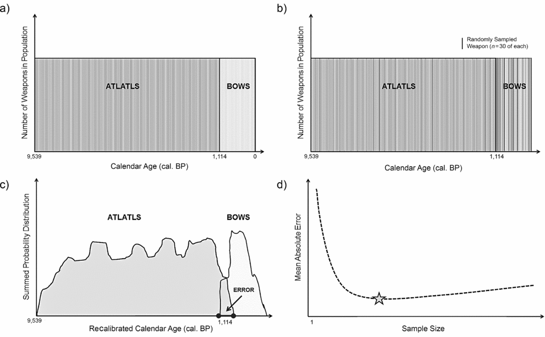
To establish minimum sample sizes, imagine a hypothetical scenario in which the number of weapons deposited yearly is constant and all weapons have an equal chance of survival regardless of age, as well as an equal chance of being sampled and dated by researchers. In this hypothetical scenario, the late Holocene transition from atlatl to bow occurred instantaneously at exactly 1114 cal BP. This produces a hypothetical population of atlatls and bows characterized by two discrete and contiguous uniform distributions within the sampling space (Figure 2a). Assume that the minimum sample size of dates required to fully represent the bow and atlatl temporal spans within this hypothetical sample space are equal.
Steps for determining minimum sample size given the sampling space and timing of the transition on the radiocarbon calibration curve. (a) Hypothetical, uniformly distributed population of atlatls and bows. (b) Randomly sampled dates for n = 30 atlatls and n = 30 bows. (c) Summed probability distributions for recalibrated “R_Simulate(_)” dates indicating overlap error measurement. (d) Mean absolute error versus sample size. The star indicates the minimum sample size, as it represents the minimum sample size at which the time span for both technologies is fully represented by the sample. Left of the star, the calibrated summed probability distributions tend to be separated. Right of the star, the calibrated summed probability distributions tend to overlap.

In order to ascertain the minimum sample size for this sample space and its estimated midpoint, the following procedure must be repeated through many iterations using various hypothetical sample sizes. Let us assume that the various sample sizes to be considered will comprise a set of n = {1, 2, 3, . . . , 100} dates on atlatls and n = {1, 2, 3, . . . , 100} dates on bows in order to produce a clear optimality curve for sample size. For the hypothetical population illustrated in Figure 2a, the actual overlap of atlatl and bow use is zero calendar years. Likewise, the separation between atlatl and bow years is zero.
In our illustrated example (Figure 2), n is equal to 30 atlatls and 30 bows. These artifacts are randomly selected from each population (Figure 2b). To simulate the process through which actual radiocarbon dates are obtained, the calendar date for each selected atlatl and bow is reverse calibrated in order to probabilistically provide a radiocarbon date plus or minus one standard error.Footnote 2 These reverse-calibrated “radiocarbon dates” are then recalibrated to calendar years and combined into summed probability distributions (Figure 2c). In this study, we re-calibrate with a conservative σ of ± 50 radiocarbon years (the mean error in the subset database is ± 44), but a larger or smaller standard error could be used if appropriate. The shape of these summed probability distributions depends on the calendar ages of the randomly sampled dates as well as their location on the radiocarbon calibration curve. Due to error and the nature of the radiocarbon calibration curve, these probability distributions inevitably overlap or are separated by some number of years on the calendar age scale. Thus, we can quantify the magnitude of the error while going through this process for each random sample as the number of years of overlap or separation present between the two summed probability distributions of the re-calibrated dates, since overlap in the hypothetical scenario was equal to zero.
This procedure is repeated 1,000 times for each sample size, n = {1, 2, 3, . . . , 100}, and the mean absolute error for each is calculated and graphed (Figure 2d). The point that minimizes sample size and minimizes the mean absolute error represents the minimum sample size (n oab). The graph's minimum represents the sample size at which the “error” between recalibrated atlatl and bow calendar ranges switches from separation to overlap, meaning that it is the sample size at which both temporal ranges are fully represented by the sample. This maximizes error predictability while minimizing overall cost and artifact sampling in cases where published radiocarbon dates do not already exist.
Additional analysis can minimize the sample size further. Recall that minimum sample size is calculated above assuming equal sample sizes of dates on bow and atlatl technology. Since the estimated atlatl time span is approximately seven times longer than the estimated bow time span, it follows that fewer bow dates are required to fully represent the bow time span. Therefore, the above procedure can be repeated by holding the atlatl sample size constant (using the minimum value for n oab [now n oa] obtained above), and iterating through possible bow sample sizes until the minimum bow sample size (n ob) is obtained.
Part 2: Determine Whether Overlap Is Significant
In Part 1, minimum sample sizes for atlatl (n oa) and bow (n ob) dates were calculated. Once adequate sample sizes of radiocarbon dates are compiled, further analysis will show whether the technologies significantly overlapped in time, or whether the transition was abrupt. This section tests the null hypothesis that there is no actual overlap in calibrated dates; any overlap observed is a product of sampling error (Supplemental Text 2).
The first step is to create a summed probability distribution for each population of actual atlatl (n a) and bow (n b) dates and calculate the number of calendar years for which the summed probability distributions overlap (positive numbers) or are separated (negative numbers). Then, we determine the actual sampling space for each technology: within what calendar range do the radiocarbon dates (± 2σ) for each technology actually fall? Finally, we estimate the sampled midpoint of the transition as the midpoint of overlap or separation in summed probability distributions.
In order to determine whether the overlap/separation in dates is significant, a probability distribution unique to this position on the radiocarbon curve and this sample size is created by repeating the following procedure over 1,000 iterations:
-
1. Given the actual sampling space and midpoint of the transition, randomly draw n a calendar dates from the atlatl range and n b calendar dates from the bow range. As before, random samples are taken from hypothetical, uniform, discrete, and contiguous atlatl and bow distributions.
-
2. Reverse calibrate (R_Simulate) these calendar dates.
-
3. Recalibrate the “radiocarbon” dates.
-
4. Calculate the amount of overlap/separation in the recalibrated dates’ summed probability distributions.
These simulated data are then used to create a histogram of modeled overlap/separation for this particular sample size and range on the radiocarbon calibration curve; the histogram estimates a probability distribution.
If the observed overlap in actual dates is greater than 95% of modeled cases where no original overlap occurred, we consider the overlap significant and reject the null hypothesis. Conversely, if the observed separation in actual dates is less than 95% of modeled cases, the atlatl and bow dates represent significantly discrete time periods and the transition likely occurred abruptly.
Part 3: If Overlap/Separation in Dates Is Significant, Determine Its Magnitude
If the overlap/separation in dates is significant, additional analysis can determine the actual temporal range of the transition, with an uncertainty estimate (Supplemental Text 2). To determine the most probable length of the transition, we construct a hypothetical population of atlatl and bow dates as above with n a and n b in the given atlatl and bow sample spaces. However, rather than constructing discrete and contiguous populations, the atlatl and bow time periods overlap in multiple runs of 1,000 iterations each for {2, 4, 6, . . . , z} calendar years.
For each of these overlapping populations, n a and n b calendar years are randomly sampled from each sample space. These calendar years are reverse calibrated to produce a radiocarbon date and recalibrated to give a calendar date. The observed amount of overlap/separation from each iteration is measured in calendar years. This process is repeated 1,000 times for each modeled amount of initial overlap between {2, 4, 6, . . . , z} years.
Model iterations at each sample size are compared to the observed “overlap” in summed probability distributions of the actual bow and atlatl radiocarbon dates. This allows us to determine how likely it is that an initial overlap of x actual calendar years would produce y years of observed overlap in the summed probability distributions. We use the compiled data from all of these runs and iterations in a simple application of Bayes’ Theorem to create a probability distribution showing the most likely length of the transition given an interval around the overlap (Supplemental Text 3).
Results
Part 1: Minimum Sample Size
In the first part of the analysis, we calculated the minimum sample size for bow and atlatl dates assuming equal numbers of dates on each technology; this result appears in Figure 3. The minimum mean absolute error occurs at a sample size of n oab = 29; therefore, the minimum sample size is n oab = 29.
This graph illustrates the minimum sample size when assuming equal sample sizes of bow and atlatl dates. Minimum sample size is 29 (circled in gray) when sample sizes are equal. Error bars represent standard error of the mean absolute error.

In the second portion of this analysis, we held sample size on atlatl technology constant at n oa = 29, while calculating the minimum bow sample size (n ob). Since the potential time span of bow technology is much shorter than that of atlatl technology, its representation requires fewer dates; the results of this analysis appear in Figure 4. Holding the sample size of atlatl dates constant while iterating through potential bow date sample sizes places the minimum mean absolute error at n ob = 19, giving the minimum sample sizes for atlatls as n oa = 29 and for bows as n ob = 19.
This graph shows the same information as Figure 3, but with a minimum atlatl sample size held constant at 29. When atlatl sample size is held constant, minimum bow sample size is further reduced to 19.

The radiocarbon dates from northwestern Subarctic Canada used in this paper (Supplemental Table 1) include 42 on diagnostic atlatl (n a) and 29 dates on diagnostic bow (n b) technologies. Therefore, both minimum sample sizes are met and exceeded.
Part 2: Is Overlap Significant?
The summed probability distributions for actual atlatl and bow dates appear in Figure 5. Using these dates, the actual sampling space for atlatls lies between 9539 and 937 cal BP. The actual sampling space for bows lies between 1403 and 0 cal BP, and the actual sampled midpoint of the transition lies at 1170 cal BP. The apparent calendric overlap in summed bow and atlatl probability distributions produced using these dates is 466 calendar years.
Summed probability distributions for actual atlatl (left) and bow (right) dates. The y-axis represents summed probability and the x-axis is the date in calendar years. This image was produced with the BChronDensity() function in program R's Bchron package. The summed probability distributions overlap for 466 years.

Randomly sampling atlatl and bow sample spaces using n a and n b over 1,000 iterations produces the estimated probability distribution shown in Figure 6. The apparent overlap of 466 summed probability distribution calendar years is greater than the overlap observed in 992/1,000 runs of a model where no initial overlap occurred. The magnitude of apparent overlap observed in summed probability distributions produced by actual bow and atlatl dates is therefore > 95% of modeled cases where no initial overlap occurred; in fact, it is actually > 99.2% of cases, so we can say with 99.2% probability that the two technologies significantly overlapped.
Probability distribution histogram with bin widths of 10 calendar years on the x-axis. This shows the amount of apparent overlap for 1,000 model runs sampling bow and atlatl dates from contiguous, uniform, non-overlapping populations with a sampled transition midpoint at 1170 cal BP. Since the observed overlap in actual dates on bows and atlatls from late Holocene Subarctic northwest Canada is greater than 99.2% of modeled cases where no initial overlap occurred, the two technologies likely overlapped in prehistory.

Part 3: Magnitude of Actual Overlap in Prehistory
Even though summed probability distributions on bow and atlatl technologies apparently overlap for 466 calibrated calendar years, this does not mean that the actual number of calendar years that they overlapped was equal to 466. The apparent overlap in summed probability distributions will be greater or less than actual calendar years of overlap because the process of collecting and calibrating radiocarbon dates inherently introduces calendric uncertainty (error) into the final dates that archaeologists are able to interpret.
Compiling data from all model runs and iterations in Part 3 yields a probability distribution showing how likely it is that {2, 4, . . . , 800} years of actual calendar overlap would produce an apparent overlap of 466 years; this probability distribution appears in Figure 7 (see Supplemental Text 3). Figure 7 shows that bow and atlatl technology likely overlapped for 174 years with one standard deviation of ± 135 years. From the probability distribution, we can compute the probability of the overlap within this one standard deviation range to be 66%. Alternatively, using the quantiles of the probability distribution, the overlap lies between 24 and 698 calendar years with 95% probability.
Probability distribution for actual years of temporal overlap between bows and atlatls during the late Holocene in Subarctic northwest Canada, based on the 466 years of apparent overlap produced by radiocarbon dates from this region. The two technologies likely overlapped for 174 ± 135 actual calendar years in (pre)history. See Supplemental Text 3 for a detailed explanation of how this probability distribution was produced.

Conclusion
The sample size of radiocarbon dates necessary to securely date and understand the nature of the transition between atlatl and bow technology depends on its position on the radiocarbon calibration curve,Footnote 3 sampling bias, population size and discard rate, and taphonomic bias. We have accounted for the first two issues in this paper. Bayesian statistics and Monte Carlo methods facilitate determining the actual meaning of radiocarbon dates on atlatl and bow technology. Computer modeling allows us to simulate the process by which radiocarbon dates are produced, sampled by archaeologists, calibrated, and subsequently interpreted.
In the northwestern Canadian Subarctic, the minimum number of dates required to understand the chronological shape of the late Holocene transition between atlatl and bow technology is 29 atlatls and 19 bows. Since 42 atlatl and 29 bow dates on diagnostic ice patch artifacts were previously published (Supplemental Table 1), these minimum sample sizes were met and exceeded. Based on our analysis, bow and atlatl technologies significantly overlapped temporally within this study region. The most likely magnitude of this overlap is 174 years (between 1257 and 1083 cal BP) with a 66% probability interval between 39 and 309 calendar years.
Understanding the nature and shape of technological transitions with greater precision will allow archaeologists to focus on times of change, rather than drawing arbitrary lines between periods and phases in prehistory. In the northwestern Canadian Subarctic, atlatl and bow technology likely co-occurred for around nine generations during the late Holocene (using a 20-year generation interval). The next question to ask is whether these technologies overlapped in space for nine generations. Bow and atlatl technology may not have been used in tandem by the same groups. Instead, perhaps it took nine generations for bows to diffuse from one portion of the study area to another. With the high-resolution temporal understanding enabled by analyses like these, we might ask whether the rate of diffusion is best explained by cultural or demic processes (e.g., Fort and Méndez Reference Fort and Méndez1999; Pinhasi et al. Reference Pinhasi, Fort and Ammerman2005). We could also, for example, test hypotheses to explain technological shifts intra- and inter-culturally under frameworks of cultural transmission (Boyd and Richerson Reference Boyd and Richerson1985; Richerson and Boyd Reference Richerson and Boyd2005) and diffusion of innovations (Rogers Reference Rogers2003) theories. Conducting detailed studies on periods of (pre)historic change is now possible through the analysis of radiocarbon date databases, the processing power of desktop computers, open-source programs such as R, and new statistical procedures developed specifically with archaeological interpretation in mind.
Acknowledgments
Thanks to Todd Surovell, Robert L. Kelly, Melissa S. Murphy, Rick Weathermon, Robert L. Bettinger, and several others for providing constructive commentary on previous drafts of this paper. We must express deep gratitude to the Canadian archaeologists who published remarkable databases of radiocarbon dates in a format that we could use and learn from. Though we may not agree on everything, Yukon archaeologists Greg Hare and Christian Thomas generously sent us helpful feedback that significantly improved our research. Pablo Gerónimo Messineo kindly translated our abstract into Spanish. Our work was partially supported by the University of Wyoming and a Jason C. Reher Memorial Fellowship, presented to the first author as part of her doctoral studies. In the spirit of this fellowship, any merits of our work are dedicated to Jason Reher's memory.
Data Availability Statement
The radiocarbon dates we used were previously published. The R code we used to run our models is attached to this paper as supplemental material.
Supplemental Materials
For supplemental material accompanying this paper, visit SAA member login at https://doi.org/10.1017/aaq.2017.53.
Supplemental Table 1. Database of radiocarbon dates used in analysis
Supplemental Text 1. Code for determining minimum sample size
Supplemental Text 2. Code for establishing probable range of overlap
Supplemental Text 3. Code for calculating the probability of observed overlap given models of known initial overlap