INTRODUCTION
Animal diseases are important from many perspectives: agricultural productivity, animal welfare, human nutrition and health and the environment. Much has been learnt from the study of animal diseases that is relevant to disease in humans, at least partly because data collection and experimentation may proceed more easily. Study of disease often has the aims of understanding, control and eradication. General principles for studying diseases are widely documented (e.g. Anderson & May Reference Anderson and May1991). However, it is perhaps endlessly arguable whether disease models for urgent practical application need to be ‘heavy-weight’ computationally, even though the mathematical principles may remain simple, or whether simpler approaches can be equally or even more effective.
In many areas of science, a range of models exists, from the simple to the highly complex model, each fulfilling a role. Simple models usually provide understanding more readily than highly detailed models, as well as being far easier to use and apply. More detailed approaches can involve stratification of age, space or both, or may represent stochasticity, possibly using Monte-Carlo simulation. Too much complexity can make a model difficult to explore and obscure qualitative insights. Indeed, urgent rapid application of a model to help control a disease outbreak may be greatly facilitated by a model of appropriate simplicity, which can also provide a valuable, although limited, understanding. As experience in parts of chemistry and physics has shown, scientific reductionism is not a tool that is to be applied mechanistically. Rather, it may be useful to find useful approximations, even constructing new intermediate levels of description, which can aid computation and facilitate joined-up thinking across a range of levels especially for real-world applications where, although realism and accuracy must be taken seriously, it should not be forgotten that understanding is often limited and the data may be sparse and uncertain from a modeller's viewpoint. An important maxim is to build the simplest model which seems able to satisfy modelling objectives and proceeds to elaborate the model only when there is a clear failure. That is, fewer pools are generally easier to handle than many; and there is preference of determinism over stochasticity until the former unequivocally fails. The availability of mathematical or computational methods does not always mean that they are needed. Indeed, their indiscriminate use may obscure important principles.
Bovine spongiform encephalopathy (BSE) or ‘mad-cow’ disease has received much attention in recent years due to outbreaks in various countries. The impact on animal health, the meat trade and farm economics is severe. Concern for better understanding and control is heightened by human health implications with the emergence of a new (variant) form of Creutzfeldt-Jakob disease (vCJD) and its possible links with BSE (Ghani Reference Ghani2002; Beghi et al. Reference Beghi, Gandolfo, Ferrarese, Rizzuto, Poli, Tonini, Vita, Leone, Logroscino, Granieri, Salemi, Savettieri, Frattola, Ru, Mancardi and Messina2004; Belay & Schonberger Reference Belay and Schonberger2005). Models of BSE epidemics have previously been reported (see below). Due to the lack of an in vivo test for infection (now remedied, see Ghani Reference Ghani2002), firm data supporting parameters and detailed model structure were often missing. Anderson et al. (Reference Anderson, Donnelly, Ferguson, Woolhouse, Watt, Udy, Mawhinney, Dunstan, Southwood, Wilesmith, Ryan, Hoinville, Hillerton, Austin and Wells1996) discuss key epidemiological processes with respect to the UK BSE epidemic. That paper was followed by a more complete analysis and account of the modelling approaches applied (Ferguson et al. Reference Ferguson, Donnelly, Woolhouse and Anderson1997). The approach is mathematically complex, combining stratification and stochasticity, with the advantages and disadvantages of such methods (see preceding paragraph). Doherr et al. (Reference Doherr, Heim, Vandevelde and Fatzer1999) modelled the expected numbers of preclinical BSE cases in Switzerland. Their model, although not explained in detail, appears to have some features in common with the model described in the current paper. Magdoń-Maksymowicz et al. (Reference Magdoń-Maksymowicz, Maksymowicz and Goldasz2006) applied cellular-automata theory to BSE propagation. The technique has been used to describe short-range interactions in dense populations. They use a half-filled 1000×1000 two-dimensional lattice of cells, with each cell being free or occupied by one item. Each time step a set of transition rules is applied. It is difficult to translate their method into what is known about BSE epidemiology. The authors state in their introduction that the approach ‘may correspond to the BSE disease propagation’. The current authors are not aware of other BSE models at a phenomenological level (e.g. such as those described by Anderson et al. Reference Anderson, Donnelly, Ferguson, Woolhouse, Watt, Udy, Mawhinney, Dunstan, Southwood, Wilesmith, Ryan, Hoinville, Hillerton, Austin and Wells1996; Ferguson et al. Reference Ferguson, Donnelly, Woolhouse and Anderson1997; Doherr et al. Reference Doherr, Heim, Vandevelde and Fatzer1999, and the model described in the current paper). Attention is now focusing more on the mechanisms of neurodegeneration (Brown Reference Brown2002), and also on modelling possible epidemics of CJD (Boëlle et al. Reference Boëlle, Thomas, Valleron, Cesbron and Will2003).
The public is presently little concerned with BSE and related diseases, owing to a perception, arguably realistic, that they are no longer a threat. However, scientifically, there are still many puzzles concerning BSE aetiology and transmission (Brown Reference Brown2002; Ghani et al. Reference Ghani, Donnelly, Ferguson and Anderson2002; Aguzzi Reference Aguzzi2006).
The objective of the current paper is to construct a very simple dynamic deterministic compartmental model of BSE and explore its behaviour thoroughly. Such a model fills an important gap in the spectrum of BSE models, contributing a biological transparency and ease of use which is not conferred by some of the models reviewed above. Indeed, the authors do not believe that more complex models (of which three have been constructed) give significantly greater insights into disease dynamics or the problems of control than simpler approaches – in fact, the contrary was the case. The model is applied to the recent UK BSE outbreak. The model captures, it is suggested, most of the relevant biology in a few meaningful parameters, and is able effectively to simulate the data on the recent UK BSE epidemic.
OVERVIEW OF BSE
The current view of BSE is as follows. A glycoprotein, called a prion protein, is widespread in the animal (in the spinal cord, brain, retina and distal ileum; Beghi et al. Reference Beghi, Gandolfo, Ferrarese, Rizzuto, Poli, Tonini, Vita, Leone, Logroscino, Granieri, Salemi, Savettieri, Frattola, Ru, Mancardi and Messina2004); it is a surface protein and, in its normal form, is designated PrPc (PrP denotes prion protein). PrPc can adopt a different pathogenic form, denoted PrPSc, known as a structural isomer. That is, PrPSc has the same amino acid sequence as PrPc but is folded into a different shape, with a decrease in alpha-helical structure and an increase in beta-sheet structure (Pan et al. Reference Pan, Baldwin, Nguyen, Gasset, Serban, Groth, Mehlhorn, Huang, Fetterick and Cohen1993). PrPSc exhibits different activities than PrPc. A neurological cell or neurone containing the normal prion form PrPc, when exposed to the isomer PrPSc, dies, and there is a conversion of PrPc to PrPSc. This leads to extensive destruction of brain tissue and death of the animal. The prion protein is not wholly inactivated by normal cooking, or the treatments which usually inactivate viruses.
Transmission of the pathological form PrPSc can, at least theoretically, occur in four ways: first via contaminated feed, involving recycling infective tissue from slaughtered cattle back into feed without adequate sterilizing treatment; second by maternal transmission; third ‘horizontally’ from another infected animal and fourth spontaneously via the incorrect folding or refolding of the normal form of prion protein PrPc to give the alternative pathological form PrPSc. The evidence is that the first of these processes was the cause of the recent UK epidemic. There is no unequivocal evidence that any of the last three mechanisms, either maternal or horizontal transmission or spontaneous (endogenous) infection, is important, although none has been ruled out (but see Cummins et al. Reference Cummins, Grace, Mcdonnell and Ward2001). No immune response, with possible recovery, is induced following infection (Aguzzi Reference Aguzzi2006).
DETERMINISTIC THREE-POOL BSE MODEL
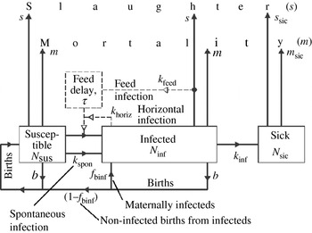
The scheme is drawn in Fig. 1. It is highly aggregated, with no representation of age of animal. The three pools (state variables) are: susceptible animals (N sus), infected animals (N inf) and clinically sick animals (N sic). The sick pool is kept at a low level by high mortality and slaughter rates (m sic, s sic).
Three-compartment BSE model. State variables are N sus (animals which are susceptible to possible infection), N inf (infected animals) and N sic (clinically sick animals). m and m sic (/year) are mortality rates applying as shown; s and s sic (/year) are slaughter rates; b (births/animal/year) is the birth rate. f binf is the fraction of births from infected animals which is infected. k feed and k horiz (/year) are infection rate constants representing infection through re-cycled feed and other horizontal infection mechanisms. τ (year) is the delay in the feed re-infection process. k spon (/year) denotes possible spontaneous infection. k inf (/year) is an incubation rate, leading to clinically sick animals.

Because animals are assumed not to recover and acquire immunity, the model cannot generate oscillations naturally as many disease simulators can. Susceptible and infected animals cannot (here) be distinguished; they are therefore assigned the same slaughter rates (s) and mortality rates (m). Similarly, the first two pools have the same birth rates (b). It is assumed that the birth rate of the sick pool is zero. Fraction f binf of births from the infected pools may be infected by maternal transmission (in the simulations reported below it is assumed that f binf=0). There is also the possibility of horizontal infection (in Fig. 1, k horiz) occurring by direct transmission from the infected pool, or via recycled feed (k feed) with a possible delay of τ (year). The latter mechanism depends on the slaughtering of infected animals. Additionally spontaneous infection is included as a possible infection route, presumably due to misfolding of prion protein (k spon). In the simulations reported here the re-cycled feed infection route is operative alone (k feed in Fig. 1), although the three other infection routes have been investigated and the results are outlined below. Disease control is achieved by cutting this re-infection pathway by making k feed=0; this essentially signals the end of the epidemic.
The three differential equations for the model are
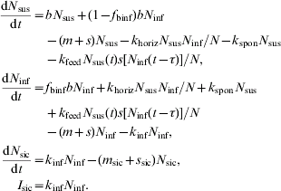
In the first differential equation for susceptibles (N sus), on the right side the terms are: births from susceptible mothers; uninfected offspring from infected mothers (f binf is the fraction of births from infected animals which are infected); mortality (m) and slaughter (s); horizontal infection (k horiz); spontaneous infection (k spon) and feed-mediated infection (k feed) with a possible delay (τ) (Fig. 1). Note that horizontal infection (k horiz) and feed-mediated infection (k feed) terms are divided by N (total number of animals, Eqns (2)); this may or may not be biologically reasonable (arguments for and against can be made), but it has the mathematical advantage of making all terms scale linearly with animal number. Solutions are then independent of animal numbers, apart from a scaling factor. In the second differential equation for infected animals, the positive terms are: births of infected offspring, horizontal infections, spontaneous infections and feed-mediated infections. The negative terms are: mortality and slaughter, and disease development (incubation) which moves infected animals (N inf) into the sick pool (N sic). The third differential equation has an input from the infected animal pool, and outputs to mortality (m sic) and slaughter (s sic). The variable I sic (animals/year), the instantaneous per year input to the sick pool, is regarded as a surrogate for the number of BSE cases reported per year, and it is explicitly defined here for simulation purposes and for comparison with data (Fig. 7).
Two auxiliary equations are required: for total animal numbers, N; and actual slaughter rate, s (which are variables, but not state variables). These are
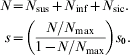
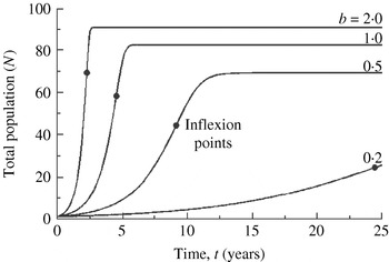
Slaughter rate s is assumed to be variable, having a small value when total population N is small, but increasing without limit as N increases towards N max, a theoretical carrying capacity, which is greater than the actual asymptote of the growth curve. This formulation gives skewed logistic-type growth (Thornley & France Reference Thornley and France2007, Section 5.4; Eqn (5.17)), towards but not achieving N max with the inflexion point closer to the asymptote than is normal for the logistic (Thornley & France Reference Thornley and France2007, pp. 715–716, 800) (Fig. 2). If N max is set to a large number, so that slaughter rates are effectively zero, then exponential growth or decline occurs. The reason for this assumption of a variable slaughter rate is that it was felt to be more realistic to simulate disease progression in an essentially static population rather than in a rapidly growing one.
Disease-free simulation of population growth as given by Fig. 1 and Eqns (1)–(3) or (5) for four values of birth rate b: 0·2, 0·5, 1 and 2/year. This gives skewed logistic-type growth of the population. Inflexion points are indicated by closed circles. Integration is by Euler's method with a fixed step of 1/128 year (1/8 year is stable and accurate enough in integration but numerical estimation of the inflexion point is not accurate enough).

Default parameters for the model
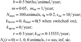
Sick animals are given a high slaughter rate (s sic). Two of the parameters in Eqns (3) (k feed and k inf) have been adjusted so that feed-mediated infection gives results close to those observed in the recent UK BSE outbreak (Fig. 7) (see the Simulation section and the discussion of Fig. 7 for details).
In the uninfected steady state, birth rate b, mortality m and slaughter rate s are related by (in Eqns (1), put dN sus/dt=0, N inf=N sic=0)

The asymptotic value of N takes a value (Eqn (6)) such that s determined by Eqns (2) satisfies Eqn (4). High birth rates b imply high slaughter rates s, natural mortality m remaining constant. Slaughter rate, and therefore birth rate, has an effect on the perceived dynamics of a BSE epidemic, because infected animals are more likely to fall sick (and therefore be counted) if the slaughter rate is low. If birth rate and hence slaughter rate are high, infected animals may be more likely to be slaughtered than to fall sick.
The growth equation for the uninfected state is (N=N sus, N inf=N sic=0; combine the first of Eqns (1) with (2))

Parameters b, m, s 0 and N max are given in Eqns (3). Equation (5) results in quasi-logistic growth.
The asymptote, N asym, as a fraction of N max, is given by (equate Eqn (5) to zero with N=N asym)
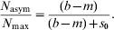
This expression approaches unity as b−m increases or s 0 decreases, and zero if b−m approaches zero or s 0 is large.
Although the inflection point of Eqn (5) for uninfected growth is defined by a quadratic, a numerical method was used for extracting the inflection point as this is generally applicable for all infected as well as uninfected conditions.
SIMULATIONS
The model was programmed in ACSL (Advanced Continuous Simulation Language, Aegis Research, Huntsville, AL), a Fortran-based non-procedural language which essentially allows Eqns (1)–(3) to be directly coded as they are. ACSL looks after the housekeeping chores of dynamic simulation, providing valuable input/output facilities and graphing, and permitting an easy interaction with the parameters representing the biology of the problem. No problems were encountered in model implementation.
Having programmed the model, the first task is to understand the impact of various parameters on dynamical responses, both of the disease-free and the diseased system (modellers sometimes find it easier to construct and program a model than to understand all ramifications of what has been assembled).
Figure 2 depicts skewed logistic-type growth in an uninfected population for four values of birth parameter, b (Eqns (3)): 0·2, 0·5, 1 and 2/year (Eqn (5)).
Respectively, the asymptotes (N asym, Eqn (6)) are 50, 69, 82 and 90 animals, compared with a maximum value of N max=100; N asym approaches N max more closely as b increases or s 0 decreases. Increasing b causes inflexion to appear earlier in time (Fig. 2), but later in the sense that it is at an increasing fraction of the asymptote. For b−m decreasing or s 0 increasing, inflexion fraction (N at inflexion/N asym) approaches 0·5, as is the case for a normal logistic equation (Thornley & France Reference Thornley and France2007). Steady-state slaughter rates are 0·15, 0·45, 0·95 and 1·95/year respectively, as determined by birth rate and mortality (Eqn (4)). Infection dynamics depends on slaughter rate, which itself depends on birth rate. Birth rate can therefore have an important effect on disease dynamics.
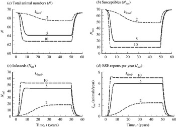
Figure 3 illustrates the infection growth curve with feed-transmitted infection (see the k feed term in the first of Eqns (1)) with a feed delay τ=0·3 year (about 3·6 months). k feed is assigned three different values, as indicated. In the simulations shown the initial total number of animals was 69·2 (the uninfected asymptote; Fig. 2, b=0·5). After 1 year, one of the uninfected animals is transferred into the infected pool, giving 68·2 susceptible animals and one infected animal in the N inf pool at time t=1 year, and k feed is assigned a non-zero value, as shown. The simulation is continued until 50 years, at which time the diseased state has come to an equilibrium. Control is applied at 50 years, by setting k feed to zero. I sic, the instantaneous number per year of new BSE cases reported, is the input into the sick box (Fig. 1, the last of Eqns (1)). This simulation procedure separates cleanly the beginning of the epidemic from the end of the epidemic, which is helpful in understanding the influence of parameters on the different phases of the disease.
Feed-mediated infection growth and decline for different values of infectivity parameter, k feed (/year; Fig. 1), as indicated. Other parameters are as in Eqns (3). After one year in the disease-free steady state (N=N sus=69·2, k feed=0; Fig. 2, b=0·5/year), infection is introduced at time t=1 year, by transferring one susceptible animal to the infected category (Fig. 1), to give t=1 year values of N sus=68·2, N inf=1, and setting k feed to a non-zero value. The delay in feed recycling is τ=0·3 year (3·6 months). After 50 years, when the infected state is in equilibrium, k feed is reset to zero to break the infection cycle. (a) Total animal numbers, N, is defined in Eqns (2). (b, c) Susceptibles N sus and infecteds N inf are state variables (Fig. 1, Eqns (1)). (d) Instantaneous number per year of new BSE reports, I sic (last of Eqns (1), the input to the sick pool) is shown. Integration is by Euler's method with a fixed step of 1/128 year.

The disease causes only a small decline (less than 10%) in total population, N (Fig. 3a), from 69·2 initially, with increasing k feed. This results from the higher (overall) mortality of infected animals (infected animals become sick, and then die or are slaughtered more quickly; Eqns (3)). The potency of feed-mediated re-infection is demonstrated in Figs 3b and 3c: increasing k feed from two to five causes a massive change in the numbers of susceptibles and infecteds. The highest value of k feed applied (10) gives an overshoot in the number of infected animals, N inf, also seen in the new BSE reports (I sic, Fig. 3d). Figure 3d plots the instantaneous value of the numbers falling sick on a per year basis (I sic, last of Eqns (1)). An important point is apparent in Fig. 3 in general and Figure 3d in particular: parameter k feed affects the leading edge of the epidemic, and not at all the trailing edge where k feed is reset to zero (even indirectly through the altered values of the state variables). Plotting the proportional rate of change of I sic makes this obvious. This result is significant when fitting the model to data.
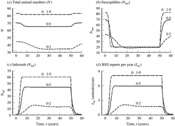
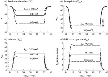
Figure 4 examines the effects of different values of birth rate b (Eqns (3)) on the dynamics of infection growth. Remember that birth rate b determines slaughter rate s (Eqn (4)), and slaughter provides infected feed, strengthening the re-infection cycle. A high slaughter rate makes it more likely that an infected animal will be slaughtered rather than fall sick (Fig. 1) and be counted. k feed is 5/year throughout. Steady-state uninfected animal numbers N depend on birth rate b (Fig. 2, Eqn (6) for N asym), decreasing with decreasing b. With disease (Fig. 4a), animal numbers decrease, the decrease increasing relatively and absolutely as b decreases, due to the increased overall death rate of infected animals. Figures 4b and 4c illustrate that the susceptibles decrease most for the higher birth rates. In the diseased steady state, the absolute number of susceptibles is approximately independent of birth rate (denoting the number of susceptibles in the diseased steady state by N sus*, it can be shown that N sus*=[N max(m+k inf)+N(s 0−m−k inf)]/(k feeds 0); for the parameters of Eqns (3), this is almost independent of N and hence birth rate b). Infected numbers increase with increasing b (Fig. 4c), as do BSE reports per year (Fig. 4d). Note that birth rate b affects both the leading and trailing edges of the epidemic. The influence of b on the trailing edge is via slaughter rate s and its effect on the emptying rate of the infected pool, N inf (Fig. 1).
Feed-mediated infection growth and decline for different values of birth rate, b (/year; Fig. 1), as indicated. Other parameters are as in Eqns (3). After one year in the disease-free steady state (N=N sus=69·2, k feed=0; Fig. 2), infection is introduced at time t=1 year, by transferring one susceptible animal to the infected category (Fig. 1), and setting k feed to 5/year. The delay in feed recycling is τ=0·3 year (3·6 months). After 50 years, when the infected state is in equilibrium, k feed is reset to zero to break the infection cycle. (a) Total animal numbers, N, is defined in Eqns (2). (b, c) Susceptibles N sus and infecteds N inf are state variables (Fig. 1, Eqns (1)). (d) Instantaneous number per year of new BSE reports, I sic (last of Eqns (1), the input to the sick pool) is shown. Integration is by Euler's method with a fixed step of 1/128 year.

Figure 5 depicts the consequences of different values of incubation rate k inf (per year) on infection dynamics. Remember that incubation time is 1/k inf so that increasing k inf is equivalent to decreasing incubation time. The default value of k inf (Eqns (3)) has been halved and doubled. Note that (Fig. 1, N inf pool) k inf competes with mortality (m) and slaughter rate (s). k inf produces the flux into the sick pool, which has higher mortality (m sic). The N inf pool, via slaughter rate s, leads to feed infection. With increasing k inf, there are small decreases of up to about 10% in total animal numbers N due to increases in overall mortality (Fig. 5a). Slaughter rate s is also decreased (not shown, but see Eqns (2) – decreased N implies decreased s). Susceptibles N sus increase greatly proportionately (Fig. 5b). Higher k inf gives rise to lower infected numbers N inf (Fig. 5c), although these lower numbers cause more BSE reports per year (Fig. 5d; see last of Eqns (1)). This is not generally the case for a more realistic model, where for instance there may be an incubation period until animals are infectious, and a second incubation up to the time when clinical sickness is observable.
Feed-mediated infection growth and decline for different values of incubation rate, k inf (/year; Fig. 1), as indicated. Other parameters are as in Eqns (3). After one year in the disease-free steady state (N=N sus=69·2, k feed=0; Fig. 2, b=0·5/year), infection is introduced at time t=1 year, by transferring one susceptible animal to the infected category (Fig. 1), to give t=1 year values of N sus=68·2, N inf=1; k feed is set to 5/year. The delay in feed recycling is τ=0·3 year (3·6 months). After 50 years, when the infected state is in equilibrium, k feed is reset to zero to break the infection cycle. (a) Total animal numbers, N, is defined in Eqns (2). (b, c) Susceptibles N sus and infecteds N inf are state variables (Fig. 1, Eqns (1)). (d) Instantaneous number per year of new BSE reports, I sic (last of Eqns (1), the input to the sick pool) is shown. Integration is by Euler's method with a fixed step of 1/128 year.

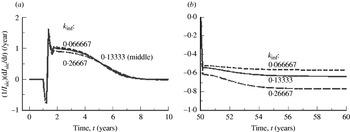
Of particular interest is the effect of incubation rate k inf on the initial and trailing edges of an epidemic (Fig. 5d). This is made clearer in Fig. 6, where the proportional rate of change of annual BSE reports is plotted until the 10th year, and for 10 years after feed infection is turned off. It is seen (Fig. 6a) that k inf has little effect on proportional growth rate: that is, it does not affect the initial stages of disease spread which is determined by other factors (feed infectivity, k feed, Fig. 3; and linked birth and slaughter rates, Fig. 4). The transient immediately after infection is introduced at time t=1 year in Fig. 6a is due to the feed infection delay of 0·3 year and is of little significance. However, k inf does very directly affect the final stages of an epidemic (Fig. 6b), after the feed infection route is broken. Note that a more complex representation, where the infected pool is divided into several sequential infected pools, in order to represent the delays after infection before an animal becomes first infectious and then sick, does not show such a simple result. In this case incubation rate k inf can influence both the leading and trailing edges of an epidemic.
As for Fig. 5 but showing the proportional rate of change in BSE reports per year for (a) the first 10 years of simulation – an infected animal is introduced at t=1 year and (b) the 10 years following the breaking of the feed-infection cycle at t=50 year when the diseased state is in equilibrium. I sic is the instantaneous per year input to the sick pool (Fig. 1; Eqns (1), last equation), which approximates the annual BSE cases reported per year. Its proportional rate of change is (1/I sic) (dI sic/dt).

The horizontal transmission route (Fig. 1) gives very similar results to feed-mediated infection; the lack of a feed delay is the only difference between these two routes.
A spontaneous infection is not generally effective unless there is also a mechanism (via feed or horizontal transmission) for amplifying the infection.
With maternally transmitted infection alone, an infection (that is, a single animal is transferred from the N sus box to the N inf box (Fig. 1) when the herd is in an equilibrium state) always dies out when the total number of animals is restricted as in Eqns (2) by parameter N max. Even for exponential growth of total animal number (simulated by making N max very large), although the number of infected animals may increase or decrease, the fraction of infected animals always decreases.
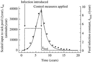
Figure 7 illustrates application of the model to data for the recent UK BSE outbreak during years 1987–2003 (quoted and used by Nowak Reference Nowak2005 who uses data supplied by the UK Department for Environment, Food and Rural Affairs). Control was applied by breaking the feed-mediated re-infection route by setting k feed=0 (instead of 5). Parameters were adjusted ‘by eye’. For the present study, this was thought to be more satisfactory than using approaches which can be insensitive to the biological meaning of key parameters (Hopkins & Leipold Reference Hopkins and Leipold1996). Least squares procedures were abandoned in the current study because linear least squares did not weight the points reasonably, and some predicted zeros caused logarithmic least squares to be unsatisfactory. Four adjustments were made to items that were considered to be adjustable or which pertained to BSE and whose values were uncertain. The fit shown in Fig. 7 was quickly obtained. Two times and two parameters were adjusted. These were: (i) the time when the infection was introduced (N inf=1 at t=1 year); (ii) the value of feed infection constant k feed when switched on at t=1 year (at the same time as infection is introduced) – this determines the initial slope of the epidemic (Fig. 3); (iii) the time (7 years) when control is applied by setting k feed=0 and the feed infection cycle is broken, marking the beginning of the end of the epidemic and last (iv) k inf, which determines the mean incubation time, equal to 1/k inf, which is known by measurement to be rather variable, but between 2 and 8 years with a mean of 5 years (Beghi et al. Reference Beghi, Gandolfo, Ferrarese, Rizzuto, Poli, Tonini, Vita, Leone, Logroscino, Granieri, Salemi, Savettieri, Frattola, Ru, Mancardi and Messina2004) – the value in the present study (Eqn (3)) is equivalent to 6 years. k inf determines the exit slope of the epidemic (Figs 5 and 6). The parameters and times are round numbers, rather than having been exhaustively tuned. Some parameters of the model (Eqns (3)), such as birth and mortality rates, b and m, slaughter parameter, s 0, and scaling parameter, N max, were regarded as fixed, outside the scope of a possible BSE epidemic, at least until the epidemic is underway and visible. Other parameters, mortality and slaughter rates of sick animals, m sic and s sic, and feed delay, τ, are not significant so long as their values are reasonable. The addition to the model of more infected pools and/or age stratification smoothes the abrupt change in slope at t=7 years, and allows more sensitive adjustments of the leading and trailing edges of the epidemic. But this extra complexity does not lead to qualitatively new behaviour or improve our general biological understanding significantly. The equivalent parameters for feed infection and for incubation, which now become vectors or matrices, modify epidemic dynamics similarly, with the exception that incubation rates can now influence the leading edge (growth rate) of the epidemic as well as the trailing edge. The fit is discussed further in the next section.
Application of 3-pool BSE model (Fig. 1) to data on the recent UK BSE outbreak. Parameters are as in Eqns (3). Two times and two of these (Eqns (3)) parameters were adjusted by eye. Initially the uninfected population is in an equilibrium state. The first time adjusted was the time when infection was introduced, set to 1 year: 1 infected animal was introduced into the N inf pool (at the same time subtracting 1 from the N sus pool and making the feed-infection rate constant k feed=5/year. The second time adjusted is the time control is simulated by making parameter k feed=0 breaking the feed-infection loop; this was set to 7 years. Parameters k feed (feed infection rate) and k inf (incubation rate) were adjusted; these affect the initial and trailing slopes of the epidemic respectively (Figs 3 and 5). The scaled input to the sick animal pool, I sic (continuous line; Eqns (1), last line), is compared to the number of cases reported per year (solid circles). A scaling factor of 7000 is applied to I sic, the input to the sick animal pool, for comparability with the data.

It should be noted that, although Fig. 7 is similar to some typical SIR epidemic curves, this is accidental. SIR denotes susceptible, infected, recovered; these categories were widely used in early epidemic modelling. Most ‘normal’ diseases require at least five categories: SIISR, denoting (1) susceptible, (2) infected but not infectious, (3) infected and now infectious, (4) sick (which may also be infectious) and (5) recovered (which are often but not always immune to re-infection). BSE has no ‘resistant’ or ‘recovered’ state (Fig. 1), which is crucial for the end phase of the usual epidemic. The shape of Fig. 7 is rather due to exponential or autocatalytic infection growth, followed by the elimination of re-infection after the cause of that re-infection (recycled feed) is switched off, with exponential decay at rate k inf.
DISCUSSION
The fit shown in Fig. 7 is satisfactory for such a basic model that, because it is easy to programme and quick to execute, is well suited for some purposes.
The way in which four of the model's parameters determine the characteristics of an epidemic is highly visible. The time when the infection is introduced defines the beginning of the epidemic. The feed infection parameter, k feed (Fig. 1; Eqns (1) and (3)) regulates the rate at which the epidemic takes hold and its intensity (Fig. 3). The beginning of the end of the epidemic is demarcated by the time when the feed re-infection loop is broken by setting k feed equal to zero. Thus the length of the epidemic is determined by the time when infection is introduced, and the time when the re-infection loop is broken. The speed with which the epidemic dies away is regulated by the incubation rate, k inf (Figs 5 and 6), which has little effect (here) on initial slope and intensity. Reasons for not adjusting other parameters have been given above. If the re-infection loop is broken before an equilibrium diseased state is established (true for Fig. 7 but not for Fig. 3), then disease intensity depends also on this time (as well as k feed).
Although the model performs quite well in terms of its predictions, current knowledge indicates that there are mechanistic limitations in the Fig. 1 representation which may not be acceptable for some applications.
A single infected pool emptying at rate constant (say) k 1 (as in Fig. 1) gives a distribution f(τ) of incubation times τ equal to k 1[exp(−k 1τ)] with a maximum at τ=0. The mean incubation time is <τ>=1/k 1. f(τ) is normalized to unity. This negative exponential distribution does not agree with observed data on incubation times (see above). Nonetheless, if the mean incubation time is about right, it is possible that predictions of an epidemic time course can be satisfactory, as indeed they seem to be (Fig. 7). With two infected pools each emptying at rate constant k 2, the first into the second and the second into the sick pool, the incubation time distribution is equal to k 22τ[exp(−k 2τ)] with a maximum at τ=1/k 2. This distribution is more realistic, being bell-shaped and zero at τ=0. The mean incubation time is <τ>=2/k 2, giving the same mean incubation time as for one pool if k 2=2k 1. Each of the two pools empties at twice the rate, so the overall transit time is unchanged. Model performance is improved, both at the level of assumptions (of incubation time distribution) and the level of predictions (of epidemic dynamics). With three infected pools each emptying at rate constant k 3, the incubation time distribution is equal to k 33τ2[exp(−k 3τ)]/2 with a maximum at τ=2/k 3. This has a sharper peak than the two-infected-pool model. The mean incubation time is <τ>=3/k 3, giving the same value as for one pool if k 3=3k 1. This process, of sequentially adding infected pools (which can also be assigned different levels of infectiousness), can be continued as far as is warranted by data and objectives. (For further discussion of the dynamics of linear compartmental systems and the gamma function, see, for example, Thornley & France Reference Thornley and France2007.) Models with one (as here), two and three infected pools were built, run and applied to the data shown in Fig. 7. A model with more infected pools can give small improvements in predictive performance, but be more realistic at the mechanistic level (of incubation time distributions: time to infectiousness and time to clinical sickness).
None of the three models mentioned above takes account of age of animal, and age of animal when infected. There is evidence that age may be important: first, susceptibility to infection (infection rate for a given exposure) may depend on age; second, once infected, the incubation characteristic may depend on the age at which infection occurred (Donnelly et al. Reference Donnelly, Ferguson, Ghani, Woolhouse, Watt and Anderson1997; Ferguson et al. Reference Ferguson, Donnelly, Woolhouse and Anderson1997; Ghani et al. Reference Ghani, Donnelly, Ferguson and Anderson2002). We also have constructed a model in which 20 age cohorts describe the population: age a=1, 2, …, 20. There are therefore 20 cohorts of susceptible animals, N sus(a). Infected animals are described by N inf (a, b), where a, as before, denotes age, and now b is age when infection occurred. b⩽a because age at infection is necessarily less than or equal to actual age. There are 210 (20×21÷2) elements in array N inf. The model can, as is the model described in detail above, be formulated using deterministic ordinary differential equations. At the predictive level, the model performs only slightly better than models with just 1-, 2- or 3-infected pools. At the mechanistic level of assumptions, the age-stratified model is now connected to reality at many more points.
The present authors do not understand the comment of Ferguson et al. (Reference Ferguson, Donnelly, Woolhouse and Anderson1997): that a deterministic compartmental approach cannot simulate different incubation period distributions. This seems unlikely because, for instance, deterministic compartments can simulate any gamma function ranging from the negative exponential up to a Dirac delta function, and surely any distribution can be decomposed into a sum of such functions. In the current work, in epidemiology and other areas, compartmental models have been used to simulate various distributions. This is of concern because others, reading the comment, may be deterred from using a deterministic compartmental approach when it could be of value, and legitimately and helpfully precedes a corresponding probabilistic model. Of course, a deterministic model can only predict determined (some sort of mean value) outcomes and these might not satisfy modelling objectives.
To refer to the stated objective (Introduction, last paragraph): a simple model, perhaps the simplest possible for this application, has been constructed; its behaviour has been thoroughly explored in Figs 2–6. Because of biological understanding of the role played by the significant parameters in the model's predictions, it was easy to ‘fit’ the model to data (Fig. 7). It is suggested that the following lessons may be learned from this exercise. For exploratory and didactic purposes a very simple model is valuable: it captures the relevant biology, and it provides a user-friendly tool. It can be completely surveyed and understood. Even for prediction of epidemic data, it is reasonable (Fig. 7). There are only four significant quantities whose adjustment is sufficient to fit the UK BSE epidemic (penultimate paragraph of Simulations section). For better quantitative agreement with data, but especially for better mechanistic representation of the underlying processes (which are being increasingly defined), a more articulated and flexible scheme may be required. This could involve, for example, recently infected, mature infected and older infected pools or, in more detail, a thorough stratification by age and age at infection. All these models have been constructed and used, and generally, experience reinforces the conclusions drawn from the model of Fig. 1 and described here. These refinements can remain deterministic, where they added little new qualitatively to the picture drawn from the investigation described in Fig. 1.
When determinism fails, then stochasticity is an option. The rate constants of a deterministic compartment model (Fig. 1; Eqns (3)), can be regarded as probabilities per unit time. The transition from determinism to stochasticity is, in principle, straightforward (e.g. Thornley & France Reference Thornley and France2007, pp. 98–101). A compartmental scheme such as Fig. 1 can be simulated deterministically or stochastically – the former is usually rather easy; the latter is mostly much more difficult to apply and interpret, but might give importantly different results (than the deterministic treatment) and be required by the problem.
The deterministic approach to modelling BSE contrasts with detailed probabilistic treatments applied (ab initio, perhaps) by other research groups (Ghani et al. Reference Ghani, Ferguson, Donnelly and Anderson2000; Huillard d'Aignaux et al. Reference Huillard, Cousens and Smith2001). When modelling, there is usually no definitive answer to the question of which is the ‘best’ modelling approach. Because models are necessarily incomplete representations of reality, they can all, to a degree, give misleading or even incorrect predictions. In addition modelling objectives vary. In modelling, whatever ‘works’, however that is defined, can have value. Nevertheless, the present authors are concerned by the propensity of parts of the modelling community to build highly sophisticated models before simpler approaches have been investigated, thoroughly understood and found wanting. Concepts are crucial for the advancement and intelligent application of science, and concepts are almost always better exposed by simpler models.
The model described above has not been ‘validated’. Validation is a demonstration that a model, within a specified domain of application, has acceptable predictive accuracy over that domain (Rykiel Reference Rykiel1996). A model may be valid for some situations (for example, Britain) and not for others (South America). Validity is not a property of the model alone. Neither is it an all-or-nothing concept; rather it lies on a scale between unity and zero. It could be difficult to design a viable protocol for a validation procedure for a disease such as BSE, where agricultural practices are so important, varied and labile. The current model has objectives of developing understanding by focussing on simplicity and transparency. Of course the model must work tolerably well when measured against data (Fig. 7). Although a real-world validation of the model would be desirable, such a validation would be impractical or almost impossible to devise. Furthermore, since the major cause of spread of the recent BSE outbreaks has been identified and agricultural industries worldwide have instigated procedures to prevent contamination of feed with infected material, it is unlikely that there will be further epidemics of BSE by this route.
Whether models can help in designing control measures is a matter for debate. Because models may not capture all important aspects of biological system, and they can therefore sometimes be wrong in unpredictable ways, models should never be used alone to design a control strategy, and any measures that models may suggest must be tempered by the views of experienced veterinarians and livestock farmers, who are au fait with current practices in an industry which is continually changing. However, models, especially of the simpler variety, are invaluable for clarifying thought and showing how parts of the system interact. They do therefore contribute to the control measure debate.
We thank Dr Bruce McNab, Office of the Chief Veterinarian for Ontario, Ontario Ministry of Agriculture Food and Rural Affairs for helpful discussions. This research was undertaken, in part, thanks to funding from the Canada Research Chairs Program.