1 Introduction
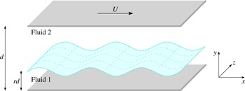
A two-layer Couette flow consists of two immiscible superposed layers of different viscous fluids confined between two horizontal plates and driven by the motion of one of the walls, as shown in figure 1. An exact steady-state solution of the Navier–Stokes equations exists with a flat interface and constant but different shear supported in each fluid region. Yih (Reference Yih1967) first showed that the flow can be linearly unstable to long waves for all non-zero Reynolds numbers, as long as the two fluids have different viscosities. The relative thicknesses and viscosities of the undisturbed layers play a crucial role and lead to the so-called thin layer effect (other parameters such as the density ratio and the surface tension being held fixed): long waves can be stabilised by placing the less viscous fluid in a relatively thin undisturbed layer, and short waves can be stabilised by a sufficient amount of surface tension (see Joseph & Renardy Reference Joseph and Renardy1992).
Following Yih’s seminal work, Hooper & Boyd (Reference Hooper and Boyd1983) focused on instabilities intrinsic to the interface by examining unbounded viscous two-fluid flows, and found that the flow is always unstable to short waves if surface tension is absent. In a related study, Hooper (Reference Hooper1985) considered the semi-infinite problem (the upper wall of the channel is moved to infinity) so that the thinner layer of fluid is always at the wall. The results reveal that the flow is always linearly stable if the lower fluid is less viscous than the upper fluid, in line with the thin layer effect. Furthermore, Hooper showed that the presence of one wall causes long-wavelength instabilities with higher growth rates than those found by Yih, confirming that the presence of a second wall on the flow is stabilising. The long-wave assumption was removed by Renardy (Reference Renardy1985, Reference Renardy1987), who solved the linear problem numerically and determined the spectrum for arbitrary flow parameters and wavenumbers. Based on the same flow configuration used by Hooper (Reference Hooper1985), Hooper & Boyd (Reference Hooper and Boyd1987) demonstrated that the semi-bounded problem can be destabilised by three types of instability. They discovered a new instability confined to the lower bounded layer, leaving the upper unbounded fluid relatively undisturbed. A ‘phase diagram’ of interfacial instabilities in two-layer Couette flows was provided by Charru & Hinch (Reference Charru and Hinch2000). The authors also proposed a physical explanation of the instabilities arising in two-layer Couette flows. In a long-wave weakly nonlinear study that retains surface tension (it needs to be asymptotically large), Hooper & Grimshaw (Reference Hooper and Grimshaw1985) derived and studied a Kuramoto–Sivashinsky equation for the interface, showing that surface tension and nonlinearity saturate the inertial instability to produce non-uniform states.
The presence of insoluble surfactants in two-fluid shear flows can induce destabilising Marangoni forces. It was shown by Frenkel & Halpern (Reference Frenkel and Halpern2002) and Halpern & Frenkel (Reference Halpern and Frenkel2003) that surfactants can produce linear instability even at zero Reynolds number (the former paper carries out a long-wavelength expansion, and the latter considers arbitrary perturbations under Stokes flow conditions). Viscosity stratification is not required (in contrast to the instability found by Yih (Reference Yih1967)) and the instability is switched off in the absence of shear or interfacial surfactant. Interestingly, the presence of a wall appears to be a necessary but not sufficient condition for the Marangoni instability – see the analysis discussion by Pozrikidis & Hill (Reference Pozrikidis and Hill2011). A recent review of Marangoni instabilities in thin films can be found in Craster & Matar (Reference Craster and Matar2009).
Geometry of the problem: two superposed fluids in a channel, driven by the motion of the upper wall with horizontal speed
 $U$
. The walls are separated by a distance
 $d$
and the flat interface is located at
 $rd$
. The wavy surface represents the disturbed interface.

The effect of inertia on the Marangoni instability of the interface was studied numerically by Pozrikidis (Reference Pozrikidis2004) and by a linear stability analysis in Blyth & Pozrikidis (Reference Blyth and Pozrikidis2004b ) for arbitrary-wavelength perturbations based on the Orr–Sommerfeld equation. The role of inertia was further investigated by Frenkel & Halpern (Reference Frenkel and Halpern2005) for perturbations of long wavelength. The results of these papers suggest that increased inertia acts to widen the range of unstable wavenumbers, making the flow more susceptible to linear instability. The findings of Frenkel and Halpern regarding Marangoni instability in the presence of insoluble surfactants were confirmed by Blyth & Pozrikidis (Reference Blyth and Pozrikidis2004a ). These authors also included the effects of gravity and surfactant surface diffusivity in a generalisation of the linear stability analysis to arbitrary wavenumbers. They also presented direct numerical simulations on relatively small periodic domains that reveal saturated nonlinear travelling wave solutions. We note that direct simulations on large domains that support intricate dynamics are quite challenging and hence dimensionally reduced models are very useful in mapping out the underlying nonlinear phenomena for wide parameter ranges. Additional nonlinear aspects of the flow using model equations valid when one of the fluid layers is thin relative to the other were carried out by Frenkel & Halpern (Reference Frenkel and Halpern2006). The authors considered waves on longer periodic domains and presented computations that indicate the disappearance of the nonlinear travelling waves predicted by Blyth & Pozrikidis (Reference Blyth and Pozrikidis2004a ). More specifically, Frenkel & Halpern (Reference Frenkel and Halpern2006) assume that the upper fluid is unbounded and derive a system of weakly nonlinear evolution equations coupling the film thickness and the local surfactant concentration in regimes where the fluid dynamics of the upper fluid does not enter into the final equations. Numerical solutions of these equations demonstrate that as the domain size is increased, the solutions become unstable to smaller wavenumber perturbations.
More recently, Bassom, Blyth & Papageorgiou (Reference Bassom, Blyth and Papageorgiou2010) considered the problem of two-layer Couette flows when the lower layer is thin compared to the upper layer and derived a pair of weakly nonlinear equations describing the coupled interfacial and surfactant dynamics. The equation contains a linear non-local integral term (a pseudo-differential operator) which couples the film and upper fluid dynamics (such non-local couplings have been found in core-annular flows also, both in the absence and presence of surfactants – see Papageorgiou, Maldarelli & Rumschitzki (Reference Papageorgiou, Maldarelli and Rumschitzki1990) and Kas-Danouche, Papageorgiou & Siegel (Reference Kas-Danouche, Papageorgiou and Siegel2009)). Numerical calculations have been carried out for a local approximation of the system (the non-local operator is approximated by a truncation of its long-wave expansion in Fourier space, making it a linear combination of partial derivatives) for asymptotically small and finite Reynolds numbers in the upper layer. For asymptotically small Reynolds number, finite-amplitude travelling waves emerge, while periodic travelling waves, chaotic solutions and complex dynamics result in the case of order-one Reynolds number. The full non-local system at asymptotically small Reynolds numbers was solved by Kalogirou, Papageorgiou & Smyrlis (Reference Kalogirou, Papageorgiou and Smyrlis2012), who found intricate dynamical phenomena (quasi-periodicity, chaos) that have not been explored in Bassom et al. (Reference Bassom, Blyth and Papageorgiou2010) (the authors showed travelling wave solutions only). Furthermore, Kalogirou et al. (Reference Kalogirou, Papageorgiou and Smyrlis2012) compared local and non-local computations with a good agreement. The present study is devoted to the nonlinear dynamics of the problem at order-one Reynolds numbers via a systematic analytical and computational study of the full non-local equations. A more recent study by Samanta (Reference Samanta2013) considers the linear problem governed by an Orr–Sommerfeld system, along with model equations derived using depth-averaging methods; our study is quite distinct from this since we consider the non-local coupling between a thin fluid layer with another layer of order-one thickness. The innovation of this work also lies in the study of the stability of three-dimensional flows via investigation of validity of a Squire’s type theorem. The stability in three-dimensions of the nonlinear travelling wave solutions observed in the two-dimensional flow is also examined.
The structure of the paper is as follows. Section 2 provides the governing equations and boundary conditions, while in § 3 the derivation of the underlying evolution equations is briefly described. In § 4 we provide the linear stability properties of the system and prove a Squire’s type theorem in the absence of inertia. We then present numerical solutions obtained by solving initial value problems; we first pursue a detailed numerical study of the two-dimensional flow in § 5 and then study the stability of one-dimensional interfacial travelling wave solutions to spanwise perturbations in § 6. We conclude by discussing our results in § 7.
2 Governing equations
Consider the flow of two immiscible, incompressible viscous fluids of equal density
 $\unicode[STIX]{x1D70C}$
in a channel of height
 $d$
, driven by the motion of the upper plate with velocity
 $U$
– see figure 1. Using Cartesian coordinates, the walls are at
 $y=0$
and
 $y=d$
, the lower fluid
 $1$
occupies
 $0<y<S(x,z,t)$
and the upper fluid
 $2$
lies in the region
 $S(x,z,t)<y<d$
;
 $y=S(x,z,t)$
is the position of the interface between the fluids and
 $t$
is time. The fluids have unequal viscosities
 $\unicode[STIX]{x1D707}_{1}$
and
 $\unicode[STIX]{x1D707}_{2}$
, and an insoluble surfactant with local concentration
 $\unicode[STIX]{x1D6E4}(x,z,t)$
is present on the interface and acts to lower the interfacial tension
 $\unicode[STIX]{x1D6FE}$
. In the undisturbed state the interface is assumed to be at
 $y=rd$
, where
 $0<r<1$
is a constant.
We non-dimensionalise lengths with
 $d$
, velocities with
 $U$
, pressures with
 $\unicode[STIX]{x1D70C}U^{2}$
, time with
 $d/U$
, surface tension by its clean value
 $\unicode[STIX]{x1D6FE}_{c}$
and the surfactant concentration by the maximum packing value
 $\unicode[STIX]{x1D6E4}_{\infty }$
. The Navier–Stokes equations in each phase
 $i=1,2$
are
 $$\begin{eqnarray}\displaystyle \frac{\unicode[STIX]{x2202}\boldsymbol{u}_{i}}{\unicode[STIX]{x2202}t}+\boldsymbol{u}_{i}\boldsymbol{\cdot }\unicode[STIX]{x1D735}\boldsymbol{u}_{i} & = & \displaystyle -\unicode[STIX]{x1D735}p_{i}+\frac{1}{Re_{i}}\unicode[STIX]{x1D6FB}^{2}\boldsymbol{u}_{i},\end{eqnarray}$$
 $$\begin{eqnarray}\displaystyle \unicode[STIX]{x1D735}\boldsymbol{\cdot }\boldsymbol{u}_{i} & = & \displaystyle 0,\end{eqnarray}$$
 $\boldsymbol{u}_{i}=(u_{i},v_{i},w_{i})^{\text{T}}$
is the velocity field and
 $Re_{i}$
are the Reynolds numbers in each fluid
 $$\begin{eqnarray}Re_{1}=\frac{\unicode[STIX]{x1D70C}Ud}{\unicode[STIX]{x1D707}_{1}},\quad Re_{2}=\frac{\unicode[STIX]{x1D70C}Ud}{\unicode[STIX]{x1D707}_{2}}=\frac{Re_{1}}{m},\end{eqnarray}$$
with
 $m=\unicode[STIX]{x1D707}_{2}/\unicode[STIX]{x1D707}_{1}$
the viscosity ratio. In addition to the no-slip conditions at the walls
 $$\begin{eqnarray}u_{1}=v_{1}=w_{1}=0\quad \text{at }y=0,\end{eqnarray}$$
 $$\begin{eqnarray}u_{2}=1,\quad v_{2}=w_{2}=0\quad \text{at }y=1,\end{eqnarray}$$
there are several boundary conditions to be imposed at the interface
 $y=S(x,z,t)$
. These are continuity of velocities
 $$\begin{eqnarray}u_{1}=u_{2},\quad v_{1}=v_{2},\quad w_{1}=w_{2}\quad \text{at }y=S(x,z,t),\end{eqnarray}$$
a kinematic condition
 $$\begin{eqnarray}v_{i}=S_{t}+u_{i}S_{x}+w_{i}S_{z},\quad i=1,2,\end{eqnarray}$$
and continuity of normal and tangential stresses
 $$\begin{eqnarray}\displaystyle & & \displaystyle \displaystyle \left[-p_{i}(1+S_{x}^{2}+S_{z}^{2})+\frac{2}{Re_{i}} (\!S_{x}^{2}u_{ix}+S_{z}^{2}w_{iz}+v_{iy}-S_{x}(u_{iy}+v_{ix})-S_{z}(v_{iz}+w_{iy})\right.\nonumber\\ \displaystyle & & \displaystyle \displaystyle \quad \left.+\,S_{x}S_{z}(u_{iz}+w_{ix})\!)\right]_{2}^{1}=\frac{(1-\unicode[STIX]{x1D6FD}\unicode[STIX]{x1D6E4})}{We}\left(\frac{(1+S_{x}^{2})S_{zz}-2S_{x}S_{z}S_{xz}+(1+S_{z}^{2})S_{xx}}{\sqrt{1+S_{x}^{2}+S_{z}^{2}}}\right),\end{eqnarray}$$
 $$\begin{eqnarray}\displaystyle & & \displaystyle \displaystyle \left[m_{i}(2S_{x}(u_{ix}-v_{iy})+S_{z}(u_{iz}+w_{ix})+S_{x}S_{z}(v_{iz}-w_{iy})+(S_{x}^{2}-1)(u_{iy}+v_{ix}))\right]_{2}^{1}\nonumber\\ \displaystyle & & \displaystyle \displaystyle \quad =Ma\,\unicode[STIX]{x1D6E4}_{x}\sqrt{1+S_{x}^{2}+S_{z}^{2}},\end{eqnarray}$$
 $$\begin{eqnarray}\displaystyle & & \displaystyle \displaystyle \left[m_{i}(2S_{z}(w_{iz}-v_{iy})+S_{x}(u_{iz}+w_{ix})+S_{x}S_{z}(u_{iy}+v_{ix})+(S_{z}^{2}-1)(v_{iz}+w_{iy}))\right]_{2}^{1}\nonumber\\ \displaystyle & & \displaystyle \displaystyle \quad =Ma\,\unicode[STIX]{x1D6E4}_{z}\sqrt{1+S_{x}^{2}+S_{z}^{2}},\end{eqnarray}$$
 $[f_{i}]_{2}^{1}=f_{1}-f_{2}$
is used. Here,
 $m_{1}=1$
,
 $m_{2}=m$
,
 $We=\unicode[STIX]{x1D70C}U^{2}d/\unicode[STIX]{x1D6FE}_{c}$
is the Weber number,
 $Ma=\unicode[STIX]{x1D6FD}/Ca$
is the Marangoni number with
 $Ca=\unicode[STIX]{x1D707}_{1}U/\unicode[STIX]{x1D6FE}_{c}$
the Capillary number. The terms
 $\unicode[STIX]{x1D6E4}_{x}$
and
 $\unicode[STIX]{x1D6E4}_{z}$
in (2.6b
) and (2.6c
), respectively, are the Marangoni forces arising from variations in the surface tension and play an important role in the dynamics. In deriving (2.6), we have assumed an equation of state
 $\unicode[STIX]{x1D6FE}=\unicode[STIX]{x1D6FE}(\unicode[STIX]{x1D6E4})$
for the dimensionless surface tension in terms of the local surfactant concentration – see Frumkin & Levich (Reference Frumkin and Levich1947), Levich (Reference Levich1962), Edwards, Brenner & Wasan (Reference Edwards, Brenner and Wasan1991). When surfactant is present in dilute concentrations, a linear Gibbs’ isotherm can be used of the form
 $$\begin{eqnarray}\unicode[STIX]{x1D6FE}=1-\unicode[STIX]{x1D6FD}\unicode[STIX]{x1D6E4},\end{eqnarray}$$
where
 $\unicode[STIX]{x1D6FD}=RT\unicode[STIX]{x1D6E4}_{\infty }/\unicode[STIX]{x1D6FE}_{c}$
is a parameter that measures the sensitivity of interfacial tension to changes in the surfactant concentration,
 $R$
is the universal gas constant and
 $T$
is the absolute temperature. Note that in the weakly nonlinear analysis that follows the use of (2.7) is fully justified. Finally, we require a conservation equation for
 $\unicode[STIX]{x1D6E4}$
and this reads (Stone & Leal Reference Stone and Leal1990; Wong, Rumschitzki & Maldarelli Reference Wong, Rumschitzki and Maldarelli1996; Li & Pozrikidis Reference Li and Pozrikidis1997)
 $$\begin{eqnarray}\displaystyle \frac{\unicode[STIX]{x2202}\unicode[STIX]{x1D6E4}}{\unicode[STIX]{x2202}t} & - & \displaystyle \frac{S_{t}}{(1+S_{x}^{2}+S_{z}^{2})}(\unicode[STIX]{x1D6E4}_{x}S_{x}+\unicode[STIX]{x1D6E4}_{z}S_{z})\nonumber\\ \displaystyle & + & \displaystyle \frac{1}{\sqrt{1+S_{x}^{2}+S_{z}^{2}}}\left[\frac{\unicode[STIX]{x2202}}{\unicode[STIX]{x2202}x}\left(\sqrt{1+S_{x}^{2}+S_{z}^{2}}u^{1}\unicode[STIX]{x1D6E4}\right)+\frac{\unicode[STIX]{x2202}}{\unicode[STIX]{x2202}z}\left(\sqrt{1+S_{x}^{2}+S_{z}^{2}}u^{2}\unicode[STIX]{x1D6E4}\right)\right]\nonumber\\ \displaystyle & + & \displaystyle \frac{\unicode[STIX]{x1D6E4}(u_{I}S_{x}-v_{I}+w_{I}S_{z})}{\sqrt{1+S_{x}^{2}+S_{z}^{2}}}\left(\frac{(1+S_{x}^{2})S_{zz}-2S_{x}S_{z}S_{xz}+(1+S_{z}^{2})S_{xx}}{\sqrt{1+S_{x}^{2}+S_{z}^{2}}}\right)\nonumber\\ \displaystyle & - & \displaystyle \frac{1}{Pe}\frac{1}{\sqrt{1+S_{x}^{2}+S_{z}^{2}}}\left[\frac{\unicode[STIX]{x2202}}{\unicode[STIX]{x2202}x}\left(\frac{\unicode[STIX]{x1D6E4}_{x}(1+S_{z}^{2})-\unicode[STIX]{x1D6E4}_{z}S_{x}S_{z}}{\sqrt{1+S_{x}^{2}+S_{z}^{2}}}\right)\right.\nonumber\\ \displaystyle & + & \displaystyle \left.\frac{\unicode[STIX]{x2202}}{\unicode[STIX]{x2202}z}\left(\frac{\unicode[STIX]{x1D6E4}_{z}(1+S_{x}^{2})-\unicode[STIX]{x1D6E4}_{x}S_{x}S_{z}}{\sqrt{1+S_{x}^{2}+S_{z}^{2}}}\right)\right]\nonumber\\ \displaystyle & = & \displaystyle 0,\end{eqnarray}$$
where
 $$\begin{eqnarray}\left.\begin{array}{@{}c@{}}\displaystyle u^{1}=\frac{(u_{I}+v_{I}S_{x})(1+S_{z}^{2})-(v_{I}S_{z}+w_{I})S_{x}S_{z}}{1+S_{x}^{2}+S_{z}^{2}},\\ \displaystyle u^{2}=\frac{(v_{I}S_{z}+w_{I})(1+S_{x}^{2})-(u_{I}+v_{I}S_{x})S_{x}S_{z}}{1+S_{x}^{2}+S_{z}^{2}},\end{array}\right\}\end{eqnarray}$$
and
 $u_{I},v_{I},w_{I}$
are the velocities at the interface. Here,
 $Pe=Ud/D_{s}$
is the Péclet number for constant surfactant diffusivity
 $D_{s}$
.
The system of equations and boundary conditions (2.1)–(2.8) admits an exact parallel flow solution
 $\boldsymbol{u}_{1}=(\overline{U}_{1}(y),0,0)$
,
 $\boldsymbol{u}_{2}=(\overline{U}_{2}(y),0,0)$
, with a flat interface at
 $y=r$
(without loss of generality,
 $\overline{P}_{1}=\overline{P}_{2}=0$
). The solution is
 $$\begin{eqnarray}\displaystyle \overline{U}_{1}=\frac{my}{r(m-1)+1},\quad \overline{U}_{2}=\frac{y+r(m-1)}{r(m-1)+1}. & & \displaystyle\end{eqnarray}$$
In what follows, we make analytical progress by developing a weakly nonlinear theory when one of the fluid layers is thin relative to the channel thickness. We describe an asymptotic theory that retains the effect of inertia in the thicker layer in order to generate dynamics that extends beyond the reach of usual lubrication theories. The resulting equations are found to be useful in describing interfacial shapes observed in experiments and this study is currently under way.
3 Derivation of the evolution equations
A detailed derivation of the evolution equations in the two-dimensional flow case was presented by Bassom et al. (Reference Bassom, Blyth and Papageorgiou2010), where the equations were analysed in the special limit of localising non-local operators in Fourier space. Our objective here is to solve the full equations and study the stability of solutions to spanwise perturbations. Hence, a brief sketch of the derivation based on a three-dimensional flow configuration is included for completeness.
The lower layer is assumed thin and has undisturbed thickness
 $r=\unicode[STIX]{x1D716}\ll 1$
. Interfacial and surfactant perturbations are introduced by
 $S(x,z,t)=\unicode[STIX]{x1D716}+\unicode[STIX]{x1D6FF}_{1}(\unicode[STIX]{x1D716})H(x,z,t)$
,
 $\unicode[STIX]{x1D6E4}(x,z,t)=\unicode[STIX]{x1D6E4}_{0}+\unicode[STIX]{x1D6FF}_{2}(\unicode[STIX]{x1D716})\unicode[STIX]{x1D6E4}^{\prime }(x,z,t)$
, with
 $\unicode[STIX]{x1D6FF}_{1}(\unicode[STIX]{x1D716}),\unicode[STIX]{x1D6FF}_{2}(\unicode[STIX]{x1D716})\ll 1$
selected to ensure coupling between the two layers and the presence of Marangoni forces at leading order. The scalings of Kas-Danouche et al. (Reference Kas-Danouche, Papageorgiou and Siegel2009) (also adopted by Bassom et al. (Reference Bassom, Blyth and Papageorgiou2010)) follow,
 $$\begin{eqnarray}\unicode[STIX]{x1D6FF}_{1}=\unicode[STIX]{x1D716}^{2},\quad \unicode[STIX]{x1D6E4}_{0}=\unicode[STIX]{x1D6FF}_{2}\unicode[STIX]{x1D6E4}_{0}^{\prime },\quad Ca=\unicode[STIX]{x1D716}Ca_{0},\quad Ma=\unicode[STIX]{x1D716}^{2}\unicode[STIX]{x1D6FF}_{2}^{-1}Ma_{0},\quad Pe=\unicode[STIX]{x1D716}^{-2}Pe_{0},\end{eqnarray}$$
where
 $\unicode[STIX]{x1D6E4}_{0}^{\prime },Ca_{0},Ma_{0},Pe_{0}$
are of
 $O(1)$
, while
 $\unicode[STIX]{x1D6FF}_{2}$
is not given a canonical scaling; it is sufficient to have
 $\unicode[STIX]{x1D6FF}_{2}\rightarrow 0$
as
 $\unicode[STIX]{x1D716}\rightarrow 0$
. The surfactant concentration scaling corresponds to the dilute limit and allows Marangoni forces to influence the nonlinear dynamics (otherwise linear dynamics ensue – Wei (Reference Wei2005)). It follows, then, that
 $\unicode[STIX]{x1D6E4}(x,z,t)=\unicode[STIX]{x1D6FF}_{2}\tilde{\unicode[STIX]{x1D6E4}}(x,z,t)$
where
 $\tilde{\unicode[STIX]{x1D6E4}}(x,z,t)=\unicode[STIX]{x1D6E4}_{0}^{\prime }+\unicode[STIX]{x1D6E4}^{\prime }$
, and this will be used as a dependent variable in the sequel. Introducing a stretched variable
 $\unicode[STIX]{x1D701}=y/\unicode[STIX]{x1D716}$
in region
 $1$
(the undisturbed interface is at
 $\unicode[STIX]{x1D701}=1$
), we expand variables there as
 $u_{1}=\overline{U}_{1}(y)+\unicode[STIX]{x1D716}^{3}U_{1}(x,\unicode[STIX]{x1D701},z,t)+\cdots \,$
,
 $v_{1}=\unicode[STIX]{x1D716}^{4}V_{1}(x,\unicode[STIX]{x1D701},z,t)+\cdots \,$
,
 $w_{1}=\unicode[STIX]{x1D716}^{3}W_{1}(x,\unicode[STIX]{x1D701},z,t)+\cdots \,$
,
 $p_{1}=\unicode[STIX]{x1D716}P_{1}(x,\unicode[STIX]{x1D701},z,t)+\cdots \,$
, while in region 2 we write
 $u_{2}=\overline{U}_{2}(y)+\unicode[STIX]{x1D716}^{2}U_{2}(x,y,z,t)+\cdots \,$
,
 $v_{2}=\unicode[STIX]{x1D716}^{2}V_{2}(x,y,z,t)+\cdots \,$
,
 $w_{2}=\unicode[STIX]{x1D716}^{2}W_{2}(x,y,z,t)+\cdots \,$
,
 $p_{2}=\unicode[STIX]{x1D716}^{2}P_{2}(x,y,z,t)+\cdots \,$
. These expansions are motivated by requiring a leading-order balance between the pressure gradient and viscous terms in the momentum equations, and continuity of velocities at the perturbed interface. Substituting these expansions into the Navier–Stokes equations (2.1) and the normal and tangential stress balances (2.6) yields, to leading order
 $$\begin{eqnarray}V_{1}|_{\unicode[STIX]{x1D701}=1}=-\frac{1}{3Ca_{0}}(H_{xxxx}+2H_{xxzz}+H_{zzzz})+\frac{Ma_{0}}{2}(\unicode[STIX]{x1D6E4}_{xx}^{\prime }+\unicode[STIX]{x1D6E4}_{zz}^{\prime })-\frac{m}{2}T|_{y=0},\end{eqnarray}$$
where
 $T(x,y,z)=U_{2xy}+V_{2xx}+V_{2zz}+W_{2zy}$
is found by solving the problem in the upper layer. Introducing the Galilean transformation
 $\tilde{x}=x-\overline{U}_{1}(\unicode[STIX]{x1D716})t$
and the slow time scale
 $\tilde{t}=\unicode[STIX]{x1D716}^{2}t$
, casts the kinematic condition (2.5) into
 $$\begin{eqnarray}H_{\tilde{t}}+mHH_{\tilde{x}}=V_{1}|_{\unicode[STIX]{x1D701}=1},\end{eqnarray}$$
while using the same transformations in the surfactant equation (2.8) yields at leading order
 $$\begin{eqnarray}\tilde{\unicode[STIX]{x1D6E4}}_{\tilde{t}}+m(H\tilde{\unicode[STIX]{x1D6E4}})_{\tilde{x}}=\frac{1}{Pe_{0}}(\tilde{\unicode[STIX]{x1D6E4}}_{\tilde{x}\tilde{x}}+\tilde{\unicode[STIX]{x1D6E4}}_{zz}).\end{eqnarray}$$
Coupling between the layers takes place through
 $T|_{y=0}$
which depends on the size of the Reynolds number in the upper layer. Inertia enters when
 $Re_{2}=O(1)$
and in what follows we use
 $R_{e}$
in place of
 $Re_{2}$
. A linearised Navier–Stokes system results at leading order; transformation into Fourier space, use of the function
 $f=-\unicode[STIX]{x2202}\hat{V}_{2}/\unicode[STIX]{x2202}y$
(hat denotes Fourier transform) and elimination of the pressure, provides
 $$\begin{eqnarray}\left(\frac{\unicode[STIX]{x2202}^{4}\hat{V}_{2}}{\unicode[STIX]{x2202}y^{4}}-2(k_{1}^{2}+k_{2}^{2})\frac{\unicode[STIX]{x2202}^{2}\hat{V}_{2}}{\unicode[STIX]{x2202}y^{2}}+(k_{1}^{2}+k_{2}^{2})^{2}\hat{V}_{2}\right)-\text{i}k_{1}R_{e}y\left(\frac{\unicode[STIX]{x2202}^{2}\hat{V}_{2}}{\unicode[STIX]{x2202}y^{2}}-(k_{1}^{2}+k_{2}^{2})\hat{V}_{2}\right)=0,\end{eqnarray}$$
which is an Orr–Sommerfeld type equation. The boundary conditions are
 $$\begin{eqnarray}\left.\begin{array}{@{}rl@{}}\displaystyle \hat{V}_{2}=0,\quad \hat{V}_{2y}=0\quad & \text{at }y=1,\\ \displaystyle \hat{V}_{2}=0,\quad \hat{V}_{2y}=-\text{i}k_{1}(m-1){\hat{H}}\quad & \text{at }y=0,\end{array}\right\}\end{eqnarray}$$
and represent no-slip at the upper wall and continuity of velocities at the interface. Writing
 $\hat{V}_{2}=-\text{i}k_{1}(m-1){\hat{H}}F(y)$
, yields the following normalised boundary value problem for
 $F(y)$
 $$\begin{eqnarray}(F^{\prime \prime \prime \prime }-2k^{2}F^{\prime \prime }+k^{4}F)-\text{i}k_{1}R_{e}y(F^{\prime \prime }-k^{2}F)=0,\end{eqnarray}$$
 $$\begin{eqnarray}F(0)=0,\quad F^{\prime }(0)=1,\quad F(1)=0,\quad F^{\prime }(1)=0,\end{eqnarray}$$
with
 $k=\sqrt{k_{1}^{2}+k_{2}^{2}}$
. Even though a solution can be written in terms of Airy functions and their integrals (see for example Hooper & Boyd (Reference Hooper and Boyd1983) and Kalogirou (Reference Kalogirou2014)), it is much more straightforward to obtain numerical solutions directly; this is achieved here using a finite difference method. Once
 $F(y;k_{1},k_{2})$
is known, we can take inverse transforms to readily obtain
 $$\begin{eqnarray}T|_{y=0}=\frac{\text{i}}{2\unicode[STIX]{x03C0}^{2}}(1-m)\int _{-\infty }^{+\infty }\int _{-\infty }^{+\infty }{\mathcal{N}}(k_{1},k_{2}){\hat{H}}(k_{1},k_{2})\text{e}^{\text{i}(k_{1}x+k_{2}z)}\,\text{d}k_{1}\,\text{d}k_{2},\end{eqnarray}$$
where
 $$\begin{eqnarray}{\mathcal{N}}(k_{1},k_{2})=-\frac{k_{1}}{2}F^{\prime \prime }(0).\end{eqnarray}$$
With
 $T|_{y=0}$
known in terms of the interfacial shape
 $H$
, (3.2) is then used in the kinematic equation (3.3), which along with the surfactant transport equation (3.4), provide the following system (with a canonical rescaling applied and the tildes dropped from all terms)
 $$\begin{eqnarray}\displaystyle & \displaystyle H_{t}+HH_{x}+\unicode[STIX]{x1D6FB}^{4}H & \displaystyle \nonumber\\ \displaystyle & \displaystyle \quad +\,\frac{\text{i}\unicode[STIX]{x1D6EC}}{4\unicode[STIX]{x03C0}^{2}}\int _{-\infty }^{+\infty }\int _{-\infty }^{+\infty }{\mathcal{N}}(k_{1},k_{2}){\hat{H}}(k_{1},k_{2})\text{e}^{\text{i}k_{1}x+\text{i}k_{2}z}\,\text{d}k_{1}\,\text{d}k_{2}-\unicode[STIX]{x1D6FB}^{2}\unicode[STIX]{x1D6E4}=0, & \displaystyle\end{eqnarray}$$
 $$\begin{eqnarray}\displaystyle & \displaystyle \unicode[STIX]{x1D6E4}_{t}+(H\unicode[STIX]{x1D6E4})_{x}-\unicode[STIX]{x1D702}\unicode[STIX]{x1D6FB}^{2}\unicode[STIX]{x1D6E4}=0. & \displaystyle\end{eqnarray}$$
The parameters
 $\unicode[STIX]{x1D6EC}$
and
 $\unicode[STIX]{x1D702}>0$
represent viscosity stratification effects and surfactant diffusivity, respectively, and are given by
 $$\begin{eqnarray}\unicode[STIX]{x1D6EC}=3Ca_{0}m(1-m),\quad \unicode[STIX]{x1D702}=\frac{3Ca_{0}}{Pe_{0}}.\end{eqnarray}$$
Note that
 $\unicode[STIX]{x1D6EC}$
is positive if
 $m<1$
, i.e. when the film is more viscous than the upper layer fluid, and negative otherwise.
For ease of representation, the non-local term was developed using Fourier transforms; nevertheless, the problem is more appropriately defined on finite domains (typically periodic of size
 $2L_{x}\times 2L_{z}$
, say), so a Fourier series representation will be used – see § 5.1. The nonlinear system (3.10)–(3.11) retains three important physical mechanisms that we wish to study in detail: shear-induced instabilities through the
 $\unicode[STIX]{x1D6EC}$
term; Marangoni effects through the
 $\unicode[STIX]{x1D6FB}^{2}\unicode[STIX]{x1D6E4}$
term in (3.10); short-wave surface tension stabilisation through the
 $\unicode[STIX]{x1D6FB}^{4}H$
term in (3.10).
Considering the two-dimensional problem, i.e. setting
 $\unicode[STIX]{x2202}_{z}=0$
,
 $k_{2}=0$
(and
 $k_{1}=k$
), the set of equations (3.10)–(3.11) is simplified by
 $$\begin{eqnarray}\displaystyle & \displaystyle H_{t}+HH_{x}+H_{xxxx}+\frac{\text{i}\unicode[STIX]{x1D6EC}}{2\unicode[STIX]{x03C0}}\int _{-\infty }^{+\infty }{\mathcal{N}}(k){\hat{H}}(k)\text{e}^{\text{i}kx}\,\text{d}k-\unicode[STIX]{x1D6E4}_{xx}=0, & \displaystyle\end{eqnarray}$$
 $$\begin{eqnarray}\displaystyle & \displaystyle \unicode[STIX]{x1D6E4}_{t}+(H\unicode[STIX]{x1D6E4})_{x}-\unicode[STIX]{x1D702}\unicode[STIX]{x1D6E4}_{xx}=0. & \displaystyle\end{eqnarray}$$
Extensive numerical computations on the above one-dimensional system were carried and are presented in a later section.
4 Linear stability analysis
We now consider the linear stability properties of the system (3.10)–(3.11). Linearising about the base state
 $H=0,\unicode[STIX]{x1D6E4}=\unicode[STIX]{x1D6E4}_{0}$
and looking for normal mode solutions proportional to
 $\text{e}^{\text{i}k_{1}x+\text{i}k_{2}z+\unicode[STIX]{x1D70E}t}$
, where
 $k_{1}$
,
 $k_{2}$
are real wavenumbers in
 $x$
- and
 $z$
-directions respectively, yields the following dispersion relation for the growth rate
 $\unicode[STIX]{x1D70E}(k_{1},k_{2})$
 $$\begin{eqnarray}\unicode[STIX]{x1D70E}^{2}+(k^{4}+\text{i}\unicode[STIX]{x1D6EC}{\mathcal{N}}(k_{1},k_{2})+\unicode[STIX]{x1D702}k^{2})\unicode[STIX]{x1D70E}+(\unicode[STIX]{x1D702}k^{6}+\text{i}\unicode[STIX]{x1D702}\unicode[STIX]{x1D6EC}{\mathcal{N}}(k_{1},k_{2})k^{2}-\text{i}\unicode[STIX]{x1D6E4}_{0}k_{1}k^{2})=0,\end{eqnarray}$$
where
 $k=\sqrt{k_{1}^{2}+k_{2}^{2}}$
. There are two modes with growth rates
 $$\begin{eqnarray}\unicode[STIX]{x1D70E}_{1,2}=-\frac{k^{4}+\text{i}\unicode[STIX]{x1D6EC}{\mathcal{N}}(k_{1},k_{2})+\unicode[STIX]{x1D702}k^{2}}{2}\pm \frac{1}{2}\sqrt{(k^{4}+\text{i}\unicode[STIX]{x1D6EC}{\mathcal{N}}(k_{1},k_{2})-\unicode[STIX]{x1D702}k^{2})^{2}+4\text{i}\unicode[STIX]{x1D6E4}_{0}k_{1}k^{2}},\end{eqnarray}$$
where the plus sign corresponds to
 $\unicode[STIX]{x1D70E}_{1}$
and the minus sign to
 $\unicode[STIX]{x1D70E}_{2}$
; instability is possible if the real part of
 $\unicode[STIX]{x1D70E}_{1}$
or
 $\unicode[STIX]{x1D70E}_{2}$
is positive, i.e. if
 $s_{1,2}=\text{Re}(\unicode[STIX]{x1D70E}_{1,2})>0$
. For equal-viscosity fluids characterised by
 $\unicode[STIX]{x1D6EC}=0$
, the growth rates in the long-wave regime
 $k_{1},k_{2}\ll 1$
are
 $$\begin{eqnarray}s_{1,2}=\pm \sqrt{\frac{\unicode[STIX]{x1D6E4}_{0}}{2}}{k_{1}}^{1/2}k-\frac{\unicode[STIX]{x1D702}}{2}k^{2}+\cdots \,,\end{eqnarray}$$
thus the flow can be unstable in this case but only in the presence of surfactant, i.e. for
 $\unicode[STIX]{x1D6E4}_{0}\neq 0$
. On the contrary, for
 $\unicode[STIX]{x1D6EC}\neq 0$
and
 $k\ll 1$
, substitution of a localisation of
 ${\mathcal{N}}(k_{1},k_{2})$
(see appendix A for details) into the dispersion relation yields
 $$\begin{eqnarray}s_{1}=\frac{(\unicode[STIX]{x1D6E4}_{0}-2\unicode[STIX]{x1D702}\unicode[STIX]{x1D6EC})}{2\unicode[STIX]{x1D6EC}}k^{2}+O(k^{3}),\quad s_{2}=\frac{(R_{e}\unicode[STIX]{x1D6EC}^{2}-30\unicode[STIX]{x1D6E4}_{0})}{60\unicode[STIX]{x1D6EC}}k_{1}^{2}-\frac{\unicode[STIX]{x1D6E4}_{0}}{2\unicode[STIX]{x1D6EC}}k_{2}^{2}+O(k^{3}).\end{eqnarray}$$
4.1 Two-dimensional perturbations
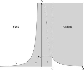
Stability diagram corresponding to two-dimensional flows, showing regions of stability (white) and instability (grey) in the
 $\unicode[STIX]{x1D6EC}-R_{e}$
parameter space. The critical points are
 $\unicode[STIX]{x1D6EC}_{c}=\unicode[STIX]{x1D6E4}_{0}/2\unicode[STIX]{x1D702}$
and
 $R_{ec}=30\unicode[STIX]{x1D6E4}_{0}/\unicode[STIX]{x1D6EC}_{c}^{2}=120\unicode[STIX]{x1D702}^{2}/\unicode[STIX]{x1D6E4}_{0}$
.

For two-dimensional perturbations, the growth rates are obtained by setting
 $k_{2}=0$
in (4.3) and (4.4) and are identical to the ones found by Bassom et al. (Reference Bassom, Blyth and Papageorgiou2010) and reduce to the ones derived by Frenkel & Halpern (Reference Frenkel and Halpern2002) and Wei (Reference Wei2005) in appropriate limits. A stability diagram showing neutral curves in
 $\unicode[STIX]{x1D6EC}-R_{e}$
parameter space is given in figure 2. Instability regions are shaded while the flow is linearly stable in the unshaded regions. One observation from the diagram is that instability always exists for
 $\unicode[STIX]{x1D6EC}=0$
at any Reynolds number, in complete agreement with the findings of Frenkel & Halpern (Reference Frenkel and Halpern2002) and Halpern & Frenkel (Reference Halpern and Frenkel2003), who found that Marangoni instability exists even for fluids with equal viscosities. Moreover, increasing
 $\unicode[STIX]{x1D6EC}>0$
destabilises the flow above the critical value
 $(30\unicode[STIX]{x1D6E4}_{0}/R_{e})^{1/2}$
(i.e. beyond the curve
 $R_{e}\unicode[STIX]{x1D6EC}^{2}=30\unicode[STIX]{x1D6E4}_{0}$
). Decreasing
 $\unicode[STIX]{x1D6EC}<0$
leads to the opposite effect; this suggests a viscosity stratification stabilisation of the Marangoni instability, as found by Kalogirou et al. (Reference Kalogirou, Papageorgiou and Smyrlis2012). Note that in the absence of surfactants (this corresponds to infinite surfactant diffusivity
 $\unicode[STIX]{x1D702}\rightarrow \infty$
and
 $\unicode[STIX]{x1D6E4}_{0}=0$
), the curves in figure 2 shrink to zero and the line
 $\unicode[STIX]{x1D6EC}=\unicode[STIX]{x1D6EC}_{c}$
coincides with the
 $\unicode[STIX]{x1D6EC}=0$
axis. In this case, the only unstable region is the first quadrant
 $\unicode[STIX]{x1D6EC}>0$
,
 $R_{e}>0$
. This is consistent with stability results for two-layer Couette flows without surfactants – it is known that the flow is linearly unstable if
 $\unicode[STIX]{x1D6EC}>0$
and
 $R_{e}>0$
, while the flow is stable for
 $\unicode[STIX]{x1D6EC}<0$
at any Reynolds number, in agreement with the results of Yih (Reference Yih1967) and Hooper (Reference Hooper1985).
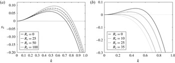
Effect of the Reynolds number on unstable growth rates of two-dimensional flows for
 $\unicode[STIX]{x1D6E4}_{0}=1$
,
 $\unicode[STIX]{x1D702}=1$
. (a) Positive
 $\unicode[STIX]{x1D6EC}=0.25$
: increasing
 $R_{e}=0,25,50,100$
leads to larger unstable region. (b) Negative
 $\unicode[STIX]{x1D6EC}=-1.0$
: increasing
 $R_{e}=0,10,25,35$
shrinks the unstable region and eventually stabilises the problem above a cutoff Reynolds number value.

Another remark is that, for
 $R_{e}=0$
, the flow is unstable as long as
 $\unicode[STIX]{x1D6EC}$
remains smaller than the critical value
 $\unicode[STIX]{x1D6EC}_{c}=\unicode[STIX]{x1D6E4}_{0}/2\unicode[STIX]{x1D702}$
, as found by Kalogirou et al. (Reference Kalogirou, Papageorgiou and Smyrlis2012). An increase in the Reynolds number stabilises the flow if
 $\unicode[STIX]{x1D6EC}<0$
and destabilises the flow if
 $\unicode[STIX]{x1D6EC}>0$
. This result is consistent with previous studies that demonstrate that inertial effects increase the growth of the Marangoni instability to produce new regions of instability, as long as the film is more viscous than the overlying fluid (Pozrikidis Reference Pozrikidis2004; Blyth & Pozrikidis Reference Blyth and Pozrikidis2004b
; Frenkel & Halpern Reference Frenkel and Halpern2005). This is also confirmed by figure 3(a) for the unstable case
 $\unicode[STIX]{x1D6EC}=0.25$
,
 $\unicode[STIX]{x1D6E4}_{0}=1$
,
 $\unicode[STIX]{x1D702}=1$
, where the growth rates are shown as functions of the wavenumber for
 $R_{e}=0,25,50,100$
. The cutoff wavenumbers below which the flow becomes stable are
 $k_{c}=0.718,0.758,0.787,0.814$
, respectively, showing that increasing inertia enhances the already present Marangoni instability, as expected. The short-wave stabilisation is due to surface tension effects (Hooper & Boyd Reference Hooper and Boyd1983), represented by the
 $H_{xxxx}$
term in the evolution equation for the film thickness (note that the large
 $k$
behaviour of
 ${\mathcal{N}}(k)\sim k^{2}$
(Kalogirou Reference Kalogirou2014) is subdominant relative to that of
 $H_{xxxx}$
). If the film is less viscous than the upper fluid, inertial effects cause stabilisation of long waves. Growth rates for
 $\unicode[STIX]{x1D6EC}=-1.0$
,
 $\unicode[STIX]{x1D6E4}_{0}=1$
,
 $\unicode[STIX]{x1D702}=1$
at different
 $R_{e}$
are given in figure 3(b), and it is seen that the growth rates decrease with increasing Reynolds numbers.
4.2 Three-dimensional perturbations
In the case of three-dimensional disturbances, a sufficient condition for instability follows if one of the growth rates in the long-wave approximations (4.4) is positive. We will discuss the cases
 $\unicode[STIX]{x1D6EC}>0$
and
 $\unicode[STIX]{x1D6EC}<0$
separately.
In the case of a more viscous film (
 $\unicode[STIX]{x1D6EC}>0$
), this is true if
 $$\begin{eqnarray}\unicode[STIX]{x1D6E4}_{0}-2\unicode[STIX]{x1D702}\unicode[STIX]{x1D6EC}>0\quad \text{or}\quad R_{e}\unicode[STIX]{x1D6EC}^{2}-30\unicode[STIX]{x1D6E4}_{0}>0.\end{eqnarray}$$
The first of conditions (4.5) can be satisfied in one of three physical ways: by either having a sufficiently large initial surfactant concentration
 $\unicode[STIX]{x1D6E4}_{0}$
, a sufficiently small surfactant diffusion coefficient
 $\unicode[STIX]{x1D702}$
or by decreasing the viscosity difference between the two fluids so that
 $\unicode[STIX]{x1D6EC}$
is small. The second condition in (4.5) is physically possible by either imposing a considerable viscosity contrast between the two fluids (i.e.
 $\unicode[STIX]{x1D6EC}$
large), by having a sufficiently large Reynolds number or by having a small initial surfactant concentration
 $\unicode[STIX]{x1D6E4}_{0}$
. Note that for three-dimensional perturbations the two neutral stability hyperbolae in figure 2 (defined by
 $R_{e}=30\unicode[STIX]{x1D6E4}_{0}/\unicode[STIX]{x1D6EC}^{2}$
in the figure), become
 $R_{e}=(30\unicode[STIX]{x1D6E4}_{0}/\unicode[STIX]{x1D6EC}^{2})(1+(k_{2}^{2}/k_{1}^{2}))$
. For non-zero values of
 $k_{2}$
these curves shift upwards (compared to the original curves that correspond to
 $k_{2}=0$
) implying that for
 $\unicode[STIX]{x1D6EC}>0$
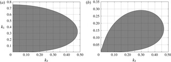
, three-dimensional perturbations are more stable than two-dimensional ones. This result is also present in figure 4(a), where the instability region is shown in the
 $k_{1}-k_{2}$
space for
 $Re=25$
,
 $\unicode[STIX]{x1D6EC}=0.25$
,
 $\unicode[STIX]{x1D6E4}_{0}=1$
,
 $\unicode[STIX]{x1D702}=1$
; we have established (data not shown) that the maximum growth occurs on the axis
 $k_{2}=0$
.
On the other hand, for
 $\unicode[STIX]{x1D6EC}<0$
this shift of the stability curves increases the region of instability, causing regions corresponding to two-dimensional stability in
 $\unicode[STIX]{x1D6EC}-R_{e}$
space (unshaded regions in figure 2) to move into the unstable grey shaded region. In particular, the point marked ‘x’ in figure 2 will now fall into the unstable region and this is also confirmed in figure 4(b), where the region of instability is portrayed for
 $Re=35$
,
 $\unicode[STIX]{x1D6EC}=-1.0$
,
 $\unicode[STIX]{x1D6E4}_{0}=1$
,
 $\unicode[STIX]{x1D702}=1$
. The choice of parameter values is such that the corresponding two-dimensional perturbations are stable (in particular, they are stable for any
 $R_{e}>30$
), and this is also seen from figure 4(b) where the instability region does not include the axis
 $k_{2}=0$
.
Unstable growth rates of three-dimensional flows showing regions of instability (grey) and stability (white) against
 $k_{1}$
,
 $k_{2}$
for
 $\unicode[STIX]{x1D6E4}_{0}=1$
,
 $\unicode[STIX]{x1D702}=1$
. (a)
 $Re=25$
,
 $\unicode[STIX]{x1D6EC}=0.25$
, corresponding to the unstable point ‘o’ on the stability diagram in figure 2. (b)
 $Re=35$
,
 $\unicode[STIX]{x1D6EC}=-1.0$
, corresponding to the stable point ‘x’ on the stability diagram in figure 2.

The above results motivate the investigation of the validity of a Squire’s type theorem in two-layer parallel flows with surfactants. In the absence of surfactants, it is known that if a three-dimensional perturbation is unstable, then a two-dimensional perturbation having the same flow parameters exists and is more unstable (Hesla, Pranckh & Preziosi Reference Hesla, Pranckh and Preziosi1986). As discussed in the previous paragraph, for order-one Reynolds numbers there exist three-dimensional perturbations that are more unstable than two-dimensional ones, hence Squire’s theorem cannot hold. The theorem holds for zero Reynolds number, however, as shown below – an alternative derivation can be found in Halpern & Frenkel (Reference Halpern and Frenkel2003). The dispersion relation (4.1) with
 $Re=0$
and use of the local system expansions (see appendix A), becomes
 $$\begin{eqnarray}\unicode[STIX]{x1D70E}^{2}+p_{1}(k_{1},k_{2})\unicode[STIX]{x1D70E}+p_{0}(k_{1},k_{2})=0,\end{eqnarray}$$
where
 $p_{0}(k_{1},k_{2})$
,
 $p_{1}(k_{1},k_{2})$
are polynomials. Denote the positive growth rate by
 $\unicode[STIX]{x1D70E}_{1}$
, i.e.
 $$\begin{eqnarray}\unicode[STIX]{x1D70E}_{1}=-\frac{p_{1}}{2}+\frac{\sqrt{p_{1}^{2}-4p_{0}}}{2}.\end{eqnarray}$$
The goal is to find the critical point
 $(k_{1}^{\ast },k_{2}^{\ast })$
where
 $\unicode[STIX]{x1D70E}_{1}$
has a local (and global) maximum. This can be done by finding the values
 $(k_{1}^{\ast },k_{2}^{\ast })$
where
 $$\begin{eqnarray}\frac{\unicode[STIX]{x2202}\unicode[STIX]{x1D70E}_{1}}{\unicode[STIX]{x2202}k_{1}}=0,\quad \frac{\unicode[STIX]{x2202}\unicode[STIX]{x1D70E}_{1}}{\unicode[STIX]{x2202}k_{2}}=0\quad \text{and}\quad \frac{\unicode[STIX]{x2202}^{2}\unicode[STIX]{x1D70E}_{1}}{\unicode[STIX]{x2202}k_{1}^{2}}\frac{\unicode[STIX]{x2202}^{2}\unicode[STIX]{x1D70E}_{1}}{\unicode[STIX]{x2202}k_{2}^{2}}-\frac{\unicode[STIX]{x2202}^{2}\unicode[STIX]{x1D70E}_{1}}{\unicode[STIX]{x2202}k_{1}k_{2}}>0,\quad \frac{\unicode[STIX]{x2202}^{2}\unicode[STIX]{x1D70E}_{1}}{\unicode[STIX]{x2202}k_{1}^{2}}<0.\end{eqnarray}$$
It can be shown that
 $\unicode[STIX]{x2202}\unicode[STIX]{x1D70E}_{1}/\unicode[STIX]{x2202}k_{2}=0$
if and only if
 $k_{2}=0$
; moreover,
 $\unicode[STIX]{x2202}\unicode[STIX]{x1D70E}_{1}/\unicode[STIX]{x2202}k_{1}=0$
for a
 $k_{1}^{\ast }\neq 0$
. At the point
 $(k_{1}^{\ast },0)$
, the second derivative criteria in (4.8) also hold, thus
 $\unicode[STIX]{x1D70E}_{1}$
has its only maximum there and its real part
 $s_{1}=\text{Re}(\unicode[STIX]{x1D70E}_{1})$
is a maximum at the same point. As an example, in the case
 $\unicode[STIX]{x1D6EC}=0.25$
,
 $\unicode[STIX]{x1D6E4}_{0}=1$
,
 $\unicode[STIX]{x1D702}=1$
, the critical point is
 $(k_{1}^{\ast },k_{2}^{\ast })\approx (0.4757,0)$
. Hence perturbations having
 $k_{2}=0$
are more unstable as shown analytically – calculations using the full dispersion relation also confirm this result. In closing, we note that at zero Reynolds number the maximum growth rate is attained at
 $k_{2}=0$
, while for order-one Reynolds numbers,
 $\unicode[STIX]{x1D70E}_{1}$
attains its maximum at wavenumbers
 $(k_{1}^{\ast },k_{2}^{\ast })\neq (0,0)$
.
5 Numerical solutions of the evolution equations
5.1 Numerical methods
The governing equations (3.10)–(3.11) are posed on
 $2L_{x}\times 2L_{z}$
-periodic domains. We begin by rescaling the evolution equations into the canonical domain
 $[0,2\unicode[STIX]{x03C0}]\times [0,2\unicode[STIX]{x03C0}]$
by applying the following transformations
 $$\begin{eqnarray}x\rightarrow \frac{L_{x}}{\unicode[STIX]{x03C0}}x,\quad z\rightarrow \frac{L_{z}}{\unicode[STIX]{x03C0}}z,\quad t\rightarrow \left(\frac{L_{x}}{\unicode[STIX]{x03C0}}\right)^{2}t,\quad H\rightarrow \frac{\unicode[STIX]{x03C0}}{L_{x}}H,\quad \unicode[STIX]{x1D6E4}\rightarrow \frac{\unicode[STIX]{x03C0}}{L_{x}}\unicode[STIX]{x1D6E4}.\end{eqnarray}$$
On
 $2\unicode[STIX]{x03C0}\times 2\unicode[STIX]{x03C0}$
-periodic domains, the non-local term in (3.10), which from now on will be denoted by
 ${\mathcal{P}}H$
, can be expressed as the following Fourier series
 $$\begin{eqnarray}{\mathcal{P}}H=\frac{\text{i}\unicode[STIX]{x1D6EC}}{\unicode[STIX]{x1D708}_{1}}\mathop{\sum }_{k_{1}=-\infty }^{+\infty }\mathop{\sum }_{k_{2}=-\infty }^{+\infty }{\mathcal{N}}(k_{1}\sqrt{\unicode[STIX]{x1D708}_{1}},k_{2}\sqrt{\unicode[STIX]{x1D708}_{2}})\widehat{H}(k_{1},k_{2})\text{e}^{\text{i}k_{1}x+\text{i}k_{2}z},\end{eqnarray}$$
where
 $$\begin{eqnarray}\widehat{H}(k_{1},k_{2})=\frac{1}{(2\unicode[STIX]{x03C0})^{2}}\int _{0}^{2\unicode[STIX]{x03C0}}\int _{0}^{2\unicode[STIX]{x03C0}}H(\unicode[STIX]{x1D709},\unicode[STIX]{x1D701},t)\text{e}^{-\text{i}k_{1}\unicode[STIX]{x1D709}-\text{i}k_{2}\unicode[STIX]{x1D701}}\,\text{d}\unicode[STIX]{x1D709}\,\text{d}\unicode[STIX]{x1D701},\end{eqnarray}$$
are the Fourier coefficients of
 $H(x,z,t)$
and
 $\unicode[STIX]{x1D708}_{1}$
,
 $\unicode[STIX]{x1D708}_{2}$
are new bifurcation parameters given by
 $$\begin{eqnarray}\unicode[STIX]{x1D708}_{1}=\left(\frac{\unicode[STIX]{x03C0}}{L_{x}}\right)^{2},\quad \unicode[STIX]{x1D708}_{2}=\left(\frac{\unicode[STIX]{x03C0}}{L_{z}}\right)^{2}.\end{eqnarray}$$
The parameters
 $\unicode[STIX]{x1D708}_{1}$
,
 $\unicode[STIX]{x1D708}_{2}$
(called ‘viscosity’ parameters in the literature), decrease as the streamwise and lateral lengths of the system
 $L_{x}$
,
 $L_{z}$
increase, and more linearly unstable modes enter into the dynamics. The transformed two-dimensional equations (corresponding to three-dimensional flows) become
 $$\begin{eqnarray}\displaystyle & \displaystyle H_{t}+HH_{x}+\left(\unicode[STIX]{x1D708}_{1}H_{xxxx}+2\unicode[STIX]{x1D708}_{2}H_{xxzz}+\frac{\unicode[STIX]{x1D708}_{2}^{2}}{\unicode[STIX]{x1D708}_{1}}H_{zzzz}\right)+{\mathcal{P}}H-\left(\unicode[STIX]{x1D6E4}_{xx}+\frac{\unicode[STIX]{x1D708}_{2}}{\unicode[STIX]{x1D708}_{1}}\unicode[STIX]{x1D6E4}_{zz}\right)=0, & \displaystyle\end{eqnarray}$$
 $$\begin{eqnarray}\displaystyle & \displaystyle \unicode[STIX]{x1D6E4}_{t}+(H\unicode[STIX]{x1D6E4})_{x}-\unicode[STIX]{x1D702}\left(\unicode[STIX]{x1D6E4}_{xx}+\frac{\unicode[STIX]{x1D708}_{2}}{\unicode[STIX]{x1D708}_{1}}\unicode[STIX]{x1D6E4}_{zz}\right)=0, & \displaystyle\end{eqnarray}$$
with
 ${\mathcal{P}}H$
given by (5.2). The corresponding one-dimensional system (for two-dimensional perturbations) becomes
 $$\begin{eqnarray}\displaystyle & \displaystyle H_{t}+HH_{x}+\unicode[STIX]{x1D708}H_{xxxx}+\frac{\text{i}\unicode[STIX]{x1D6EC}}{\unicode[STIX]{x1D708}}\mathop{\sum }_{k=-\infty }^{+\infty }{\mathcal{N}}(k\sqrt{\unicode[STIX]{x1D708}}){\hat{H}}(k)\text{e}^{\text{i}kx}-\unicode[STIX]{x1D6E4}_{xx}=0, & \displaystyle\end{eqnarray}$$
 $$\begin{eqnarray}\displaystyle & \displaystyle \unicode[STIX]{x1D6E4}_{t}+(H\unicode[STIX]{x1D6E4})_{x}-\unicode[STIX]{x1D702}\unicode[STIX]{x1D6E4}_{xx}=0, & \displaystyle\end{eqnarray}$$
where
 $\unicode[STIX]{x1D708}=(\unicode[STIX]{x03C0}/L)^{2}$
.
The systems (5.5)–(5.6) and (5.7)–(5.8) are discretised in space using spectral methods and in time by implicit–explicit BDF (Backward Differentiation Formula) schemes with as much as sixth-order accuracy where desired – see Akrivis et al. (Reference Akrivis, Kalogirou, Papageorgiou and Smyrlis2016). All the results reported here were obtained using a second-order BDF scheme; for completeness, details of the scheme and its implementation for system (5.7)–(5.8) can be found in appendix B. It is straightforward to generalise the method to system (5.5)–(5.6).
5.2 Computational study for two-dimensional flows
This section presents results from a large number of numerical experiments that aim to elucidate the nonlinear dynamics of the one-dimensional system (5.7)–(5.8). We use several computational diagnostic tools to monitor and identify the different attractors obtained numerically. The use of such tools is essential, mainly due to the complexity of the dynamics, non-uniqueness of solutions and large number of bifurcations (for example, we wish to be able to identify whether a solution is chaotic or quasi-periodic in time). One useful tool is the energy
 $E(t)$
of the solution
 $H(x,t)$
, defined by the
 $L_{2}$
-norm
 $$\begin{eqnarray}E(t):=\Vert H(\cdot ,t)\Vert _{2}^{2}=\int _{0}^{2\unicode[STIX]{x03C0}}H^{2}(x,t)\,\text{d}x.\end{eqnarray}$$
The quadrature is performed with spectral accuracy (either using Parseval’s identity or trapezoidal quadrature), and
 $E(t)$
can be used in highly accurate phase-plane constructions (
 $E(t),{\dot{E}}(t)$
) and Poincaré maps (or return maps) satisfying
 ${\dot{E}}(t)=0$
. Such data analyses are useful in characterising the dynamical behaviour of the system, as seen later. To uniformly maintain accuracy, the calculation of
 ${\dot{E}}(t)$
also needs to be carried out with spectral accuracy (a low-order finite difference formula in time is not good enough). We achieve this by multiplying (5.7) by
 $H$
and integrating over a period, to find
 $$\begin{eqnarray}{\dot{E}}(t)=-2\unicode[STIX]{x1D708}\Vert H_{xx}\Vert _{2}^{2}-2\int _{0}^{2\unicode[STIX]{x03C0}}H({\mathcal{P}}H)\,\text{d}x+2\int _{0}^{2\unicode[STIX]{x03C0}}H\unicode[STIX]{x1D6E4}_{xx}\,\text{d}x.\end{eqnarray}$$
All integrals on the right-hand side of (5.10) can be computed with spectral accuracy once the Fourier coefficients of
 $H$
and
 $\unicode[STIX]{x1D6E4}$
are found. Next, the values of the minima (and maxima) of the energy
 $E(t)$
and the times of their occurrence are estimated from the discrete time series using a second-order polynomial interpolation in time. Denoting the minima (maxima) by the set
 $E_{n},n=1,2,\ldots \,$
, we construct return maps by plotting the points
 $(E_{n},E_{n+1})$
,
 $n=1,2,\ldots \,$
, in the plane. The resulting geometrical object provides information about the attractor. If the return map contains
 $m$
isolated points, the flow is time-periodic with
 $m$
minima in the signal of
 $E(t)$
; the time period of the oscillations is estimated by calculating the time difference between
 $(m+1)$
consecutive minima. Continuous-looking curves that fill up with points as
 $n$
increases indicate quasi-periodic behaviour (analogous to flow on a torus), while foldings and geometrical self-similarity provide strong evidence for chaos – see Bergé, Pomeauc & Vidal (Reference Bergé, Pomeauc and Vidal1984) for such techniques used in physical experiments; numerical experiments have an advantage over physical experiments in that the data sets can be both much larger and also much more accurate.
For parameter values that support travelling wave solutions, the phase speed
 $c$
is calculated numerically by assuming wave solutions of permanent form given by
 $H(x,t)=H(x-ct)$
,
 $\unicode[STIX]{x1D6E4}(x,t)=\unicode[STIX]{x1D6E4}(x-ct)$
. We can calculate
 $c$
by computing the solutions at large times; if a travelling wave of permanent form emerges, then
 $c$
is given by
 $$\begin{eqnarray}c=\limsup _{t\rightarrow \infty }\frac{\displaystyle \int _{0}^{2\unicode[STIX]{x03C0}}\unicode[STIX]{x1D6E4}_{x}(H\unicode[STIX]{x1D6E4})_{x}\,\text{d}x}{\displaystyle \int _{0}^{2\unicode[STIX]{x03C0}}\unicode[STIX]{x1D6E4}_{x}^{2}\,\text{d}x}.\end{eqnarray}$$
Once again, the integrals in (5.11) can be calculated with spectral accuracy using Parseval’s theorem.
The initial conditions used in all reported simulations (unless stated otherwise) are
 $$\begin{eqnarray}H(x,0)={\textstyle \frac{1}{10}}\unicode[STIX]{x1D708}^{-1/2}\sin x,\quad \unicode[STIX]{x1D6E4}(x,0)=\unicode[STIX]{x1D6E4}_{0}\unicode[STIX]{x1D708}^{-1/2}.\end{eqnarray}$$
The factor
 $\unicode[STIX]{x1D708}^{-1/2}$
is used to ensure that for simulations performed for different
 $\unicode[STIX]{x1D708}$
with all other parameters fixed, the undisturbed physical film thickness and base surfactant concentration are the same irrespective of the unscaled domain length
 $2L$
(recall the transformation (5.1)).
All the results that follow in this section were calculated for initial surfactant concentration
 $\unicode[STIX]{x1D6E4}_{0}=1$
and surfactant diffusion coefficient
 $\unicode[STIX]{x1D702}=1$
. The equal viscosity flow having
 $\unicode[STIX]{x1D6EC}=0$
was studied first to confirm the results of Bassom et al. (Reference Bassom, Blyth and Papageorgiou2010). Our main interest lies in identifying the effect of the non-local term and the effect of the presence of inertia on the dynamics. To that end, hundreds of numerical experiments were carried out for different values of
 $\unicode[STIX]{x1D708}$
,
 $R_{e}$
and
 $\unicode[STIX]{x1D6EC}\neq 0$
. For
 $R_{e}=0$
, the flow is found to be stable for
 $\unicode[STIX]{x1D708}\geqslant 0.516$
, in complete agreement with Kalogirou et al. (Reference Kalogirou, Papageorgiou and Smyrlis2012). For
 $R_{e}\neq 0$
, the flow is unstable if
 $\unicode[STIX]{x1D6EC}<0.5$
or
 $R_{e}\unicode[STIX]{x1D6EC}^{2}>30$
when the film is more viscous (
 $\unicode[STIX]{x1D6EC}>0$
), or if
 $R_{e}\unicode[STIX]{x1D6EC}^{2}<30$
when the upper fluid is more viscous (
 $\unicode[STIX]{x1D6EC}<0$
). Numerical solution of the dispersion relation indicates that instability occurs below a critical value
 $\unicode[STIX]{x1D708}_{c}$
that depends on the values of
 $R_{e}$
and
 $\unicode[STIX]{x1D6EC}$
.
Dynamical behaviour of the solutions for decreasing values of
 $\unicode[STIX]{x1D708}$
, for
 $R_{e}=25$
,
 $\unicode[STIX]{x1D6EC}=0.25$
,
 $\unicode[STIX]{x1D6E4}_{0}=1$
,
 $\unicode[STIX]{x1D702}=1$
. Key to solution types: ST – stable flow; TW – travelling waves;
 $\text{PTW}[m]$
– time-periodic travelling waves with
 $m$
distinct minima in the
 $E(t)$
signal per time period; QP – quasi-periodic oscillations in time; C – chaotic oscillations in time.

5.2.1 Upper (thicker) layer less viscous,
 $\unicode[STIX]{x1D6EC}>0$

We begin with a typical case
 $R_{e}=25$
,
 $\unicode[STIX]{x1D6EC}=0.25$
, for which the flow is linearly unstable for
 $\unicode[STIX]{x1D708}<0.575$
. For
 $\unicode[STIX]{x1D708}\geqslant 0.575$
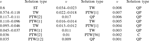
, large-time solutions tend to trivial steady states and non-trivial dynamics arises below this value. The results of extensive large-time computations for different values of
 $\unicode[STIX]{x1D708}$
are displayed in table 1 for the range
 $0.01\leqslant \unicode[STIX]{x1D708}\leqslant 0.6$
. The different attractors identified in the table are: TW – travelling waves of permanent form;
 $\text{PTW}[m]$
– periodic travelling waves that undergo time-periodic oscillations with
 $m$
distinct minima in the energy signal
 $E(t)$
(these are waves that after each period of oscillation return to their original form but are shifted spatially by a constant amount); QP – quasi-periodic oscillations in time; C – chaotic oscillations in time.
Coupled flow for
 $R_{e}=25$
,
 $\unicode[STIX]{x1D6EC}=0.25$
,
 $\unicode[STIX]{x1D6E4}_{0}=1$
,
 $\unicode[STIX]{x1D702}=1$
. (a) Interfacial (solid) and surfactant (dotted)
 $L_{2}$
-norms for
 $\unicode[STIX]{x1D708}=0.2$
. (b) Phase plane of the energy
 $E(t)$
for
 $\unicode[STIX]{x1D708}=0.1$
.

For values of
 $\unicode[STIX]{x1D708}$
close to (and smaller than) the bifurcation point
 $\unicode[STIX]{x1D708}_{c}=0.575$
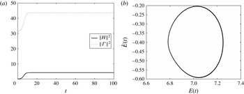
and for a relatively broad range of values, the solutions saturate to steady-state travelling waves; oscillations in the energy signal (if they exist) decay and the norms reach constant values. An example of this behaviour is provided in figure 5(a) for
 $\unicode[STIX]{x1D708}=0.2$
and it is seen that travelling waves are strongly attracting in the sense that they emerge relatively quickly in time. At
 $\unicode[STIX]{x1D708}\approx 0.117$
a Hopf bifurcation occurs giving rise to time-periodic travelling waves. As
 $\unicode[STIX]{x1D708}$
decreases from
 $0.117$
to
 $0.111$
, the energy
 $E(t)$
has two minima over its time period. At
 $\unicode[STIX]{x1D708}\approx 0.11$
another bifurcation occurs with time oscillations supporting one minimum in every period. These bifurcations can be identified by considering the energy phase plane that tends to a closed curve (periodic cycle) after a large time, as shown in figure 5(b) for
 $\unicode[STIX]{x1D708}=0.1$
. As
 $\unicode[STIX]{x1D708}$
decreases further, travelling wave solutions are interchanged with time-periodic solutions with the pattern persisting until
 $\unicode[STIX]{x1D708}\approx 0.017$
. For
 $\unicode[STIX]{x1D708}=0.017$
we find that the large-time solutions converge to a quasi-periodic attractor. To indicate the complexity of the solutions as
 $\unicode[STIX]{x1D708}$
decreases further, we note that for
 $\unicode[STIX]{x1D708}=0.01$
the flow is periodic and
 $56$
distinct isolated points can be identified in the return map – the energy
 $E(t)$
has
 $56$
local minima. As
 $\unicode[STIX]{x1D708}$
becomes even smaller, e.g.
 $\unicode[STIX]{x1D708}\leqslant 0.009$
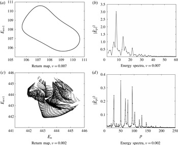
, the flow gets attracted to complex dynamical behaviour that is mainly quasi-periodic but also chaotic. Figure 6 illustrates return maps and the corresponding energy spectra for
 $\unicode[STIX]{x1D708}=0.007$
(a,b) and
 $\unicode[STIX]{x1D708}=0.002$
(c,d). The return map for
 $\unicode[STIX]{x1D708}=0.007$
consists of a continuous curve topologically equivalent to a circle (cf. flow on a torus) confirming quasi-periodicity, while for
 $\unicode[STIX]{x1D708}=0.002$
foldings in the return map are found and these suggest that the flow is chaotic.
Return maps and corresponding energy spectra for
 $\unicode[STIX]{x1D708}=0.007$
(a) and (b) and
 $\unicode[STIX]{x1D708}=0.002$
(c) and (d), for
 $R_{e}=25$
,
 $\unicode[STIX]{x1D6EC}=0.25$
,
 $\unicode[STIX]{x1D6E4}_{0}=1$
,
 $\unicode[STIX]{x1D702}=1$
. In the panels presenting the spectra of the energy signal,
 $|\hat{E}_{p}|^{2}$
denotes the Fourier coefficients found by taking an FFT (fast Fourier transform) of the energy signal in time. The results show complex dynamical phenomena, namely quasi-periodicity (results in (a,b)) and chaos (results in (c,d)).

Representative plots of the interfacial height
 $H$
(solid curve) and local surfactant concentration
 $\unicode[STIX]{x1D6E4}$
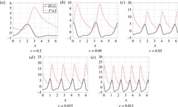
(dashed curve) are provided in figure 7 for all computed windows where travelling waves are found. In the first window which supports travelling waves (
 $0.118\leqslant \unicode[STIX]{x1D708}\leqslant 0.574$
), the waves are fully modal, i.e. all Fourier modes are present and the spatial period is
 $2\unicode[STIX]{x03C0}$
. Figure 7(a) shows typical solutions from this window for
 $\unicode[STIX]{x1D708}=0.2$
. In the second travelling wave window (
 $0.046\leqslant \unicode[STIX]{x1D708}\leqslant 0.095$
) the solutions become bimodal, i.e. their Fourier spectrum contains only even wavenumbers and the spatial period is
 $\unicode[STIX]{x03C0}$
, as illustrated in figure 7(b) for the case of
 $\unicode[STIX]{x1D708}=0.09$
. As
 $\unicode[STIX]{x1D708}$
decreases further, the travelling wave windows
 $0.023\leqslant \unicode[STIX]{x1D708}\leqslant 0.034$
,
 $0.014\leqslant \unicode[STIX]{x1D708}\leqslant 0.016$
and
 $\unicode[STIX]{x1D708}=0.011$
support waves that are tri-, tetra- and penta-modal, respectively, i.e. their basic spatial periods are
 $2\unicode[STIX]{x03C0}/3$
,
 $\unicode[STIX]{x03C0}/2$
and
 $2\unicode[STIX]{x03C0}/5$
and their non-zero Fourier modes are multiples of
 $3,4$
and
 $5$
, respectively. Figure 7(c–e) illustrates such solutions for
 $\unicode[STIX]{x1D708}=0.03$
,
 $\unicode[STIX]{x1D708}=0.015$
and
 $\unicode[STIX]{x1D708}=0.011$
. The results of figure 7 also show that as
 $\unicode[STIX]{x1D708}$
is reduced the amplitudes of the interfacial waves as well as the surfactant concentration increase. In fact their increase is proportional to
 $\unicode[STIX]{x1D708}^{-1/2}$
as found in our computations (Kalogirou Reference Kalogirou2014), confirming that the unscaled amplitudes remain of order one as seen from the transformation (5.1).
Wave profiles
 $H(x)$
(solid) and
 $\unicode[STIX]{x1D6E4}(x)$
(dashed) at time
 $t=100$
, for
 $R_{e}=25$
,
 $\unicode[STIX]{x1D6EC}=0.25$
,
 $\unicode[STIX]{x1D6E4}_{0}=1$
,
 $\unicode[STIX]{x1D702}=1$
. Each panel corresponds to an
 $n$
-modal travelling wave with spatial period
 $2\unicode[STIX]{x03C0}/n$
,
 $n=1,\ldots ,5$
, respectively.

Another notable feature of the solutions presented in figure 7 is that the surfactant concentration attains a local maximum or minimum in the vicinity of points where
 $H=0$
(this feature also appears in figure 10 presented later). To explain this physically we consider the total velocity at the interface
 $u_{I}=\overline{U}_{I}(\unicode[STIX]{x1D716})+m\unicode[STIX]{x1D716}^{2}H+\unicode[STIX]{x1D716}^{3}U_{1}+O(\unicode[STIX]{x1D716}^{4})$
, which shows that the leading-order perturbation of order
 $O(\unicode[STIX]{x1D716}^{2})$
is equal to
 $mH$
. This in turn implies that in the frame of reference moving with the undisturbed interfacial velocity, the horizontal velocity changes sign at points
 $x^{\ast }$
where
 $H(x^{\ast })=0$
– the point
 $x^{\ast }$
is a local stagnation point, to leading order and in the moving frame. The flow is inwards towards
 $x^{\ast }$
if
 $H^{\prime }(x^{\ast })<0$
and outwards if
 $H^{\prime }(x^{\ast })>0$
; in the former case the inwards flow sweeps surfactant to the vicinity of
 $x^{\ast }$
and so provides a local increase in surfactant concentration leading to a maximum in
 $\unicode[STIX]{x1D6E4}$
there – see figure 10 for regions ahead of local maxima of
 $H$
. When
 $H^{\prime }(x^{\ast })>0$
the flow sweeps surfactant away from
 $x^{\ast }$
and hence leads to a local minimum in
 $\unicode[STIX]{x1D6E4}$
(i.e. a depletion of surfactant) just behind local maxima of
 $H$
. Similar findings were reported in a study of surfactant-laden core-annular flows by Kas-Danouche et al. (Reference Kas-Danouche, Papageorgiou and Siegel2009).
5.2.2 Upper (thicker) layer more viscous,
$\unicode[STIX]{x1D6EC}<0$

We begin by presenting solutions for
 $\unicode[STIX]{x1D6EC}=-0.25$
, for which the flow is unstable for Reynolds numbers
 $R_{e}<480$
– we fix
 $R_{e}=25$
. For these parameters the flow is linearly unstable for
 $\unicode[STIX]{x1D708}<0.55$
and the solutions are mostly travelling waves of permanent form, except for
 $0.049\leqslant \unicode[STIX]{x1D708}\leqslant 0.053$
where the solutions are time-periodic travelling waves. Numerical calculations were performed for
 $\unicode[STIX]{x1D708}$
as small as
 $0.01$
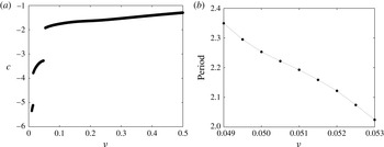
, but no intricate structures were observed (i.e. quasi-periodicity or chaos). In figure 8(a) the variation of the wave speed
 $c$
with
 $\unicode[STIX]{x1D708}$
is shown for all computed windows where travelling waves of permanent form emerge, while figure 8(b) depicts the variation of the period of oscillation with
 $\unicode[STIX]{x1D708}$
for solutions in the time-periodic window. It is seen that the travelling wave speed is monotonically decreasing as
 $\unicode[STIX]{x1D708}$
deceases, while in the case of time-periodic travelling waves the period of oscillation increases monotonically as
 $\unicode[STIX]{x1D708}$
decreases. The breaks in the curves of figure 8(a) are due to the existence of different solution branches at the same parameter values (this is caused by the nonlinearity – see Kevrekidis, Nicolaenko & Scovel (Reference Kevrekidis, Nicolaenko and Scovel1990) for a detailed bifurcation study of the various solutions of the Kuramoto–Sivashinsky equation).
Characteristics of (a) travelling wave speeds, and (b) periods of oscillation for time-periodic travelling waves, for
 $R_{e}=25$
,
 $\unicode[STIX]{x1D6EC}=-0.25$
,
 $\unicode[STIX]{x1D6E4}_{0}=1$
,
 $\unicode[STIX]{x1D702}=1$
.

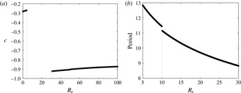
Effect of the Reynolds number
 $R_{e}$
on (a) travelling wave speeds and (b) periods of oscillation for time-periodic travelling waves, for
 $\unicode[STIX]{x1D708}=0.1$
,
 $\unicode[STIX]{x1D6EC}=0.25$
,
 $\unicode[STIX]{x1D6E4}_{0}=1$
,
 $\unicode[STIX]{x1D702}=1$
.

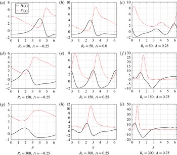
Representative wave profiles
 $H(x)$
(solid) and
 $\unicode[STIX]{x1D6E4}(x)$
(dashed) for different values of
 $\unicode[STIX]{x1D6EC}$
and
 $R_{e}=50$
(a–c),
 $R_{e}=150$
(d–f),
 $R_{e}=300$
(g–i) and
 $\unicode[STIX]{x1D708}=0.1$
,
 $\unicode[STIX]{x1D6E4}_{0}=1$
,
 $\unicode[STIX]{x1D702}=1$
.

Next we consider the effect of the Reynolds number on the characteristics of the flow for fixed
 $\unicode[STIX]{x1D708}$
(i.e. fixed domain size). We took the representative value
 $\unicode[STIX]{x1D708}=0.1$
and performed numerical calculations for the range of Reynolds numbers
 $0\leqslant R_{e}\leqslant 100$
. We find that solutions develop into travelling waves for the ranges
 $0\leqslant R_{e}\leqslant 4$
and
 $31\leqslant R_{e}\leqslant 100$
; the variation of the travelling wave speed
 $c$
with
 $R_{e}$
is shown in figure 9(a). As can be seen from the figure, no travelling waves emerge for the range
 $5\leqslant R_{e}\leqslant 30$
; the solutions here are time-periodic travelling waves instead and their period of oscillation is depicted in figure 9(b). The travelling waves on either side of the time-periodic window belong to different bifurcation branches, as confirmed by inspection of figure 9(a). Interestingly, the time-periodic travelling wave window is also split into two distinct branches above and below
 $R_{e}\approx 10$
. Our initial value problem computations converge to the most attracting solutions, and we have confirmed this numerically by starting with different initial conditions from (5.12) (namely
 $H(x,0)=\unicode[STIX]{x1D708}^{-1/2}(\sin x+0.5\cos 2x)/10$
,
 $\unicode[STIX]{x1D6E4}(x,0)=\unicode[STIX]{x1D6E4}_{0}\unicode[STIX]{x1D708}^{-1/2}$
), in which case we obtain different travelling wave solutions at the same parameters – a numerical bifurcation study can fully map out such structures but this is not pursued further here. An overall physical feature of the results is that the wave speed
 $c$
is negative and increases with the Reynolds number, at least where stable travelling waves exist. Furthermore, the period of oscillation of time-periodic travelling waves (where they are supported) is found to decrease monotonically with the Reynolds number.
We conclude this section by presenting solution features from different regions of the stability diagram 2. To fix matters we take
 $\unicode[STIX]{x1D6E4}_{0}=1$
,
 $\unicode[STIX]{x1D702}=1$
which in turn provide the critical values
 $\unicode[STIX]{x1D6EC}_{c}=0.5$
and
 $R_{ec}=120$
(recall from figure 2 that the flow can be linearly stable if
 $\unicode[STIX]{x1D6EC}>\unicode[STIX]{x1D6EC}_{c}$
and
 $R_{e}<R_{ec}$
or if
 $\unicode[STIX]{x1D6EC}<0$
and
 $R_{e}>R_{ec}$
). To quantify the effect of the Reynolds number and viscosity ratio on the flow, we computed the large-time solutions for a range of
 $R_{e}$
and
 $\unicode[STIX]{x1D6EC}$
. Here, we consider three different Reynolds numbers
 $R_{e}=50,150,300$
and for each one we compute the large-time behaviour of the solutions for three values of
 $\unicode[STIX]{x1D6EC}$
from the linearly unstable region (the shaded area) in figure 2. The computed solutions are travelling waves in all nine cases and are depicted in figure 10. Figure 10(a–c) corresponds to
 $R_{e}=50<R_{ec}=120$
and
 $\unicode[STIX]{x1D6EC}=-0.25$
(a),
 $\unicode[STIX]{x1D6EC}=0$
(b),
 $\unicode[STIX]{x1D6EC}=0.25<\unicode[STIX]{x1D6EC}_{c}=0.5$
(c), with each panel showing the interfacial profile (solid curve) and the corresponding local surfactant concentration (dashed curve). The amplitude of the interfacial profile increases when
 $\unicode[STIX]{x1D6EC}$
varies from
 $-0.25$
to
 $0$
, but then decreases again when
 $\unicode[STIX]{x1D6EC}$
changes to
 $0.25$
. In fact it is found that as
 $\unicode[STIX]{x1D6EC}$
gets closer to the critical value
 $\unicode[STIX]{x1D6EC}_{c}=0.5$
, the solution amplitudes decrease to zero. Such non-monotonic behaviour has also been computed in the case
 $R_{e}=0$
(see Kalogirou et al. (Reference Kalogirou, Papageorgiou and Smyrlis2012) and the bifurcation diagram in their figure 3b). An additional feature when inertia is present, is that a sufficiently large
 $\unicode[STIX]{x1D6EC}$
produces a non-trivial travelling wave solution as expected from the stability diagram in figure 2 (we have confirmed that a travelling wave emerges when
 $\unicode[STIX]{x1D6EC}=0.8$
– another branch of bifurcating travelling waves will start at
 $\unicode[STIX]{x1D6EC}\approx \sqrt{3/5}$
). At the value
 $R_{e}=150$
which is above the critical
 $R_{ec}$
, an increase in
 $\unicode[STIX]{x1D6EC}$
to positive values does not suppress the instability as in the previous case that supports a stability window; results are shown in figure 10(d–f) for the values
 $\unicode[STIX]{x1D6EC}=-0.25$
(d),
 $\unicode[STIX]{x1D6EC}=0.25$
(e) and
 $\unicode[STIX]{x1D6EC}=0.75$
(f). These results indicate that the wave amplitudes increase with
 $\unicode[STIX]{x1D6EC}$
– in fact the interfacial amplitudes are approximately equal to
 $3$
,
 $5$
and
 $17$
for
 $\unicode[STIX]{x1D6EC}$
equal to
 $-0.25$
,
 $0.25$
and
 $0.75$
, respectively. Figure 10(g–i) corresponds to
 $R_{e}=300$
with
 $\unicode[STIX]{x1D6EC}=-0.25$
(g),
 $\unicode[STIX]{x1D6EC}=0.25$
(h) and
 $\unicode[STIX]{x1D6EC}=0.75$
(i); once again we can conclude that the solution amplitudes increase as
 $\unicode[STIX]{x1D6EC}$
increases, analogously to the case of a lower
 $R_{e}$
. Another observation supported by our results is that for a fixed
 $\unicode[STIX]{x1D6EC}<0$
, the amplitudes of the solutions decrease as
 $R_{e}$
increases since in this case the Reynolds number has a stabilising effect on the flow – for example, see the results for
 $\unicode[STIX]{x1D6EC}=-0.25$
in figure 10(a,d,g). On the other hand, if
 $\unicode[STIX]{x1D6EC}>0$
and fixed, increasing the Reynolds number leads to an increase in the solution amplitudes (see the panels corresponding to
 $\unicode[STIX]{x1D6EC}=0.25$
in figure 10
c,f,i); such behaviour is consistent with the linear stability results summarised in figure 2.
6 Emergence of three-dimensional flows due to secondary spanwise instabilities
In the numerical results presented above we have shown that nonlinear travelling waves can be found for different values of the parameters
 $\unicode[STIX]{x1D708}$
,
 $R_{e}$
and
 $\unicode[STIX]{x1D6EC}$
. Physically, the system may also be susceptible to spanwise perturbations, and it is important to establish whether computed one-dimensional interfacial coherent structures are stable. In what follows we consider the stability (to spanwise perturbations) of travelling waves of the form
 $\overline{H}(\unicode[STIX]{x1D709})$
and
 $\overline{\unicode[STIX]{x1D6E4}}(\unicode[STIX]{x1D709})$
, where
 $\unicode[STIX]{x1D709}=x-ct$
and
 $c$
is the speed of propagation. Note that such waves are stable to streamwise disturbances in the
 $x$
-direction (of wavelengths no longer than the computational period) since they are computed as large-time solutions of initial value problems. One-dimensional interfacial travelling waves are characterised by a constant energy at large times and analogous diagnostics are used for three-dimensional flows by defining the energy
 $$\begin{eqnarray}\Vert H(\cdot ,\cdot ,t)\Vert _{2}^{2}=\int _{0}^{2\unicode[STIX]{x03C0}}\int _{0}^{2\unicode[STIX]{x03C0}}H^{2}(x,z,t)\,\text{d}x\,\text{d}z.\end{eqnarray}$$
We first investigate the linear stability of one-dimensional interfacial travelling wave solutions to three-dimensional disturbances by writing
 $$\begin{eqnarray}H(\unicode[STIX]{x1D709},z,t)=\overline{H}(\unicode[STIX]{x1D709})+\tilde{H}(\unicode[STIX]{x1D709},z,t),\quad \unicode[STIX]{x1D6E4}(\unicode[STIX]{x1D709},z,t)=\overline{\unicode[STIX]{x1D6E4}}(\unicode[STIX]{x1D709})+\tilde{\unicode[STIX]{x1D6E4}}(\unicode[STIX]{x1D709},z,t).\end{eqnarray}$$
Linearising with respect to tilde quantities and looking for solutions in the form
 $$\begin{eqnarray}\tilde{H}=f(\unicode[STIX]{x1D709})\text{e}^{\unicode[STIX]{x1D706}t}\text{e}^{\text{i}k_{2}z},\quad \tilde{\unicode[STIX]{x1D6E4}}=g(\unicode[STIX]{x1D709})\text{e}^{\unicode[STIX]{x1D706}t}\text{e}^{\text{i}k_{2}z},\end{eqnarray}$$
where
 $f(\unicode[STIX]{x1D709})$
and
 $g(\unicode[STIX]{x1D709})$
are
 $2\unicode[STIX]{x03C0}$
-periodic yields the following coupled system of ordinary differential equations to determine the eigenvalue
 $\unicode[STIX]{x1D706}$
,
 $$\begin{eqnarray}\displaystyle \unicode[STIX]{x1D706}f+(\overline{H}f)_{\unicode[STIX]{x1D709}}+\unicode[STIX]{x1D708}_{1}\left(\unicode[STIX]{x2202}_{\unicode[STIX]{x1D709}}^{2}-\frac{\unicode[STIX]{x1D708}_{2}}{\unicode[STIX]{x1D708}_{1}}k_{2}^{2}\right)^{2}f+\widehat{{\mathcal{P}}}_{k_{2}}f-\left(\unicode[STIX]{x2202}_{\unicode[STIX]{x1D709}}^{2}-\frac{\unicode[STIX]{x1D708}_{2}}{\unicode[STIX]{x1D708}_{1}}k_{2}^{2}\right)g & = & \displaystyle 0,\end{eqnarray}$$
 $$\begin{eqnarray}\displaystyle \unicode[STIX]{x1D706}g+(\overline{H}g)_{\unicode[STIX]{x1D709}}+(\overline{\unicode[STIX]{x1D6E4}}f)_{\unicode[STIX]{x1D709}}-\unicode[STIX]{x1D702}\left(\unicode[STIX]{x2202}_{\unicode[STIX]{x1D709}}^{2}-\frac{\unicode[STIX]{x1D708}_{2}}{\unicode[STIX]{x1D708}_{1}}k_{2}^{2}\right)g & = & \displaystyle 0.\end{eqnarray}$$
 $\widehat{{\mathcal{P}}}_{k_{2}}$
is the Fourier transform of the pseudo-differential operator
 ${\mathcal{P}}$
with respect to
 $z$
. The system is next cast into a matrix problem that can be readily used to compute the eigenvalues, by representing
 $f(\unicode[STIX]{x1D709})$
and
 $g(\unicode[STIX]{x1D709})$
in terms of their Fourier coefficients (this is also done for
 $\overline{H}(\unicode[STIX]{x1D709})$
and
 $\overline{\unicode[STIX]{x1D6E4}}(\unicode[STIX]{x1D709})$
which have known Fourier coefficients). The Fourier series are truncated appropriately to provide a finite-dimensional eigenvalue problem for
 $\unicode[STIX]{x1D706}(k_{2};\unicode[STIX]{x1D708}_{1},\unicode[STIX]{x1D708}_{2},R_{e},\unicode[STIX]{x1D6EC},\unicode[STIX]{x1D6E4}_{0},\unicode[STIX]{x1D702})$
, which is then solved for integer values of
 $k_{2}$
(for every value of
 $k_{2}\in \mathbb{Z}_{+}$
, a stability curve similar to figure 3 is obtained). If the real part of
 $\unicode[STIX]{x1D706}$
is positive for any
 $k_{2}$
, then instability is supported for spanwise perturbations of wavelength
 $2\unicode[STIX]{x03C0}/k_{2}$
(note that due to translational invariance in the
 $x$
-direction,
 $\unicode[STIX]{x1D706}=0$
is always an eigenvalue). In practice, since the system is long-wave unstable, setting
 $k_{2}=1$
and looking for at least one
 $\unicode[STIX]{x1D706}$
with positive real part is a sufficient condition for spanwise instability.
The analysis described above was first used to study the stability of the nonlinear one-dimensional interfacial travelling wave solution branches given in figure 9(a). The spectra were computed to establish (results not given for brevity) that both branches are linearly unstable to spanwise disturbances. Rather than presenting eigenvalue plots, we have followed the instabilities into the nonlinear regime to compute the two-dimensional solutions that arise. We solve the partial differential equations (PDEs) (5.5)–(5.6) subject to initial conditions
 $$\begin{eqnarray}H(x,z,0)=\overline{H}(\unicode[STIX]{x1D709})+{\mathcal{R}}(z),\quad \unicode[STIX]{x1D6E4}(x,z,0)=\overline{\unicode[STIX]{x1D6E4}}(\unicode[STIX]{x1D709})+{\mathcal{R}}(z),\end{eqnarray}$$
where
 $$\begin{eqnarray}{\mathcal{R}}(z)=\mathop{\sum }_{m=1}^{N}(\unicode[STIX]{x1D6FC}_{m}\sin mz+\unicode[STIX]{x1D6FD}_{m}\cos mz),\end{eqnarray}$$
and
 $\unicode[STIX]{x1D6FC}_{m},\unicode[STIX]{x1D6FD}_{m}\in [-0.1,0.1]$
are random Fourier coefficients; in the runs presented here we also pick
 $N=5$
– larger wavenumbers are damped significantly so this choice is appropriate. Typical results were computed for
 $\unicode[STIX]{x1D708}_{1}=\unicode[STIX]{x1D708}_{2}=0.1$
and
 $R_{e}=75,85,95$
(other parameters are as in figure 9
a), and the results are shown in figure 11. Figure 11(a–c) shows the unstable one-dimensional interfacial travelling waves
 $\overline{H}(\unicode[STIX]{x1D709})$
, while (d–f) provides the stable two-dimensional interfacial travelling waves at the three different values of
 $R_{e}$
.
Interfacial profiles for
 $\unicode[STIX]{x1D708}=0.1$
,
 $\unicode[STIX]{x1D6EC}=0.25$
,
 $\unicode[STIX]{x1D6E4}_{0}=1$
,
 $\unicode[STIX]{x1D702}=1$
and
 $R_{e}=75$
(a,d),
 $R_{e}=85$
(b,e),
 $R_{e}=95$
(c,f). The profiles in (a–c) are obtained from the one-dimensional initial value problem with the initial conditions (5.12). (d–f) Depict fully two-dimensional interfacial solutions for
 $\unicode[STIX]{x1D708}_{1}=\unicode[STIX]{x1D708}_{2}=0.1$
.

We also found that the flow can be linearly unstable to spanwise perturbations for several other choices of the parameter values. We illustrate the underlying instabilities by presenting numerical solutions of the nonlinear evolution equations (5.5)–(5.6) for the three set of parameter values corresponding to the marked points in figure 2. The first set of results are for
 $Re=25$
,
 $\unicode[STIX]{x1D6EC}=0.25$
,
 $\unicode[STIX]{x1D6E4}_{0}=1$
,
 $\unicode[STIX]{x1D702}=1$
. These parameters correspond to the point ‘o’ in the stability diagram in figure 2 – here the flat uniform state is unstable to streamwise perturbations and nonlinear travelling waves
 $\overline{H}(\unicode[STIX]{x1D709})$
and
 $\overline{\unicode[STIX]{x1D6E4}}(\unicode[STIX]{x1D709})$
arise. These travelling waves are computed by solving the one-dimensional equations (5.7)–(5.8) with
 $\unicode[STIX]{x1D708}=0.2$
, in order to find
 $\overline{H}(\unicode[STIX]{x1D709})$
and
 $\overline{\unicode[STIX]{x1D6E4}}(\unicode[STIX]{x1D709})$
to be used in (6.5) (more precisely, the travelling waves are recorded at
 $t=2000$
, long after any transient dynamics). Perturbations in the
 $z$
-direction are added according to (6.5)–(6.6) and new initial value problems are solved by fixing
 $\unicode[STIX]{x1D708}_{1}=0.2$
and taking decreasing values of
 $\unicode[STIX]{x1D708}_{2}$
starting from
 $\unicode[STIX]{x1D708}_{2}=0.2$
, i.e. starting from a wave on a square domain, and allowing the unscaled spanwise period to increase as
 $\unicode[STIX]{x1D708}_{2}$
decreases. We find that until approximately
 $\unicode[STIX]{x1D708}_{2}=0.06$
, the nonlinear solution is stable to spanwise disturbances and remains independent of
 $z$
. As
 $\unicode[STIX]{x1D708}_{2}$
decreases below
 $0.06$
, spanwise modes become unstable and two-dimensional interfacial travelling wave solutions emerge in the direction of the underlying flow. An example of such a solution is given for
 $\unicode[STIX]{x1D708}_{2}=0.03$
(in unscaled terms the wave dimensions are approximately
 $14\times 36$
units) in figures 12(a) and (b), which show the evolution of the energy (6.1) and the interfacial profile
 $H$
at
 $t=2000$
, respectively. As
 $\unicode[STIX]{x1D708}_{2}$
is decreased further a Hopf bifurcation takes place that leads to time-periodic travelling waves as can be seen by the case
 $\unicode[STIX]{x1D708}_{2}=0.0085$
(an unscaled domain of dimensions
 $14\times 68$
, approximately), shown in figure 12(c–d). The time-periodicity can be seen from the energy signal in (c) and the three-dimensionality of the flow is clearly identified by the interfacial profile in (d), selected at
 $t=2000$
.
Energy of two-dimensional solutions (a,c) and interfacial profiles (b,d) for
 $Re=25$
,
 $\unicode[STIX]{x1D6EC}=0.25$
,
 $\unicode[STIX]{x1D6E4}_{0}=1$
,
 $\unicode[STIX]{x1D702}=1$
. (a,b)
 $\unicode[STIX]{x1D708}_{1}=0.2$
,
 $\unicode[STIX]{x1D708}_{2}=0.03$
: interfacial travelling wave. (c,d)
 $\unicode[STIX]{x1D708}_{1}=0.2$
,
 $\unicode[STIX]{x1D708}_{2}=0.0085$
: time-periodic interfacial travelling wave. Both profiles are taken at time
 $t=2000$
.

The three-dimensionality of the flow was also quantified by calculating the difference of the
 $L_{2}$
-norms of the travelling wave profiles supported for every
 $\unicode[STIX]{x1D708}_{2}$
,
 $$\begin{eqnarray}d(H,\overline{H})=\Vert H(x,z,t)\Vert ^{2}-\Vert \overline{H}(\unicode[STIX]{x1D709})\Vert ^{2}.\end{eqnarray}$$
The results are shown in figure 13 as a function of
 $\unicode[STIX]{x1D708}_{2}^{-1}$
for those values of
 $\unicode[STIX]{x1D708}_{2}$
which support travelling wave solutions. For
 $0.06\leqslant \unicode[STIX]{x1D708}_{2}\leqslant 0.2$
the measure
 $d(H,\overline{H})=0$
, confirming that the travelling waves remain one-dimensional. For
 $\unicode[STIX]{x1D708}_{2}<0.06$
, two-dimensional interfacial waves emerge and become more pronounced as
 $\unicode[STIX]{x1D708}_{2}$
decreases. This pattern continues until
 $\unicode[STIX]{x1D708}_{2}\approx 0.03$
, below which a Hopf bifurcation takes place as discussed earlier.
Measure of three-dimensionality defined in (6.7) for
 $\unicode[STIX]{x1D708}_{1}=0.2$
and
 $Re=25$
,
 $\unicode[STIX]{x1D6EC}=0.25$
,
 $\unicode[STIX]{x1D6E4}_{0}=1$
,
 $\unicode[STIX]{x1D702}=1$
.

When
 $\unicode[STIX]{x1D6EC}<0$
, i.e. the less viscous liquid is in the thin layer, the base state in the absence of surfactants is linearly stable to two-dimensional perturbations but can be unstable in their presence. Such a case is noted on figure 2 with a star symbol for the parameters
 $Re=25$
,
 $\unicode[STIX]{x1D6EC}=-0.25$
,
 $\unicode[STIX]{x1D6E4}_{0}=1$
,
 $\unicode[STIX]{x1D702}=1$
and a computation of the evolution equations (5.7)–(5.8) with
 $\unicode[STIX]{x1D708}=0.25$
produces nonlinear one-dimensional interfacial travelling waves as expected. Even though the base state is stable to three-dimensional perturbations on a square domain at these parameter values, the one-dimensional interfacial travelling waves can lose stability to sufficiently long spanwise perturbations (equivalently if
 $\unicode[STIX]{x1D708}_{2}$
is sufficiently small in our scaled system (5.5)–(5.6)). The emerging solutions are travelling waves in the direction of the flow with two-dimensional interfacial and surfactant distributions. These results are illustrated in figure 14 for the parameters given above; (a) depicts the one-dimensional travelling wave interface (extended in the spanwise direction for illustration purposes) while (b) shows the large-time solution that results by perturbing this for
 $\unicode[STIX]{x1D708}_{2}=0.01$
. Both solutions are taken at
 $t=2000$
units which is sufficiently large for transients to die out. The three-dimensionality is clearly discernible and the profiles are qualitatively similar to those for
 $\unicode[STIX]{x1D6EC}=0.25$
given in figure 12.
Interfacial wave profiles for
 $Re=25$
,
 $\unicode[STIX]{x1D6EC}=-0.25$
,
 $\unicode[STIX]{x1D6E4}_{0}=1$
,
 $\unicode[STIX]{x1D702}=1$
. (a)
 $\unicode[STIX]{x1D708}=0.25$
: one-dimensional travelling wave due to surfactant-induced instability. (b)
 $\unicode[STIX]{x1D708}_{1}=0.25$
,
 $\unicode[STIX]{x1D708}_{2}=0.01$
: three-dimensional flow with a two-dimensional interfacial travelling wave profile. All profiles are taken at time
 $t=2000$
and travel along the
 $x$
-axis.

Finally, we consider cases for which the base flow is stable to two-dimensional linear perturbations but unstable to three-dimensional ones. As discussed already in § 4.2, in the presence of surfactants Squire’s theorem does not hold for order-one Reynolds numbers and we wish to follow such three-dimensional instabilities into the nonlinear regime. The example we select has parameters
 $Re=35$
,
 $\unicode[STIX]{x1D6EC}=-1.0$
,
 $\unicode[STIX]{x1D6E4}_{0}=1$
and
 $\unicode[STIX]{x1D702}=1$
– this is represented by a symbol ‘x’ in the two-dimensional stability diagram in figure 2 and is seen to be in the stable region. One-dimensional interfacial travelling wave solutions do not emerge in this case (at least for all initial conditions tested here – this is expected if the initial conditions are not too large) and computations are carried out by perturbing the flat base state. A representative example is given in figure 15 for
 $\unicode[STIX]{x1D708}_{1}=\unicode[STIX]{x1D708}_{2}=0.05$
(a square domain of size
 $28\times 28$
, approximately). Figure 15(a) shows the evolution of the energy norms of the interface and the surfactant concentration (
 $\Vert H\Vert ^{2}$
and
 $\Vert \unicode[STIX]{x1D6E4}\Vert ^{2}$
, respectively), while (b) and (c) show the corresponding profiles at
 $t=100$
, after the transient phase. The waves travel at an angle of
 $45^{\circ }$
relative to the base flow and are seen to be one-dimensional in the rotated frame, i.e. they are functions of
 $x+z-ct$
where
 $c$
is the speed of propagation. The emergence of these non-trivial waves for a set of parameter values that produce trivial solutions in two-dimensional flows can be explained by the shift of the stability curve in figure 2, producing a larger region of instability for
 $\unicode[STIX]{x1D6EC}<0$
(see the discussion in § 4) so that the point marked ‘x’ now falls into the unstable (grey) region.
 $L_{2}$
-norms and profiles showing interfacial shape and surfactant concentration at
 $t=100$
. The parameter values used are
 $\unicode[STIX]{x1D708}_{1}=\unicode[STIX]{x1D708}_{2}=0.05$
and
 $Re=35$
,
 $\unicode[STIX]{x1D6EC}=-1.0$
,
 $\unicode[STIX]{x1D6E4}_{0}=1$
,
 $\unicode[STIX]{x1D702}=1$
. The corresponding two-dimensional flow is stable.

It should be stressed that all of the two-dimensional interfacial solutions presented above are stable to perturbations that are no longer than the basic period in either the streamwise or spanwise direction. It would be interesting to consider longer wave perturbations to establish if the solutions are also modulationally stable, something that has not been addressed for multi-dimensional Kuramoto–Sivashinsky (KS) type equations (for the one-dimensional KS equation the reader is referred to Frisch, She & Thual (Reference Frisch, She and Thual1986), Papageorgiou, Papanicolaou & Smyrlis (Reference Papageorgiou, Papanicolaou, Smyrlis, Caflisch and Papanicolaou1992) and Barker et al. (Reference Barker, Johnson, Noble, Miguel Rodrigues and Zumbrun2013)). This is left for future investigations.
7 Conclusions
In this paper, the problem of two-layer Couette flows in the presence of surfactants is tackled analytically and numerically. Asymptotic analysis is used to derive a set of evolution equations for the interfacial shape and the local surfactant concentration on the interface. The analysis assumes that one of the layers is thin and that weakly nonlinear waves form with wavelengths that scale with the channel thickness. An interaction between the thin and thick layers produces a non-local coupling into the interfacial dynamics; the coupling arises by solving an Orr–Sommerfeld type problem in the thick layer that is valid at arbitrary (but not asymptotically large) Reynolds numbers. Two- and three-dimensional flows are considered and evolution equations are derived in both cases. The dynamical behaviour of the system is explored by undertaking extensive computations for a wide range of parameter values.
The non-local models derived here retain all salient physical mechanisms associated with two-fluid shear flows as we briefly list next. These include the inertial long-wave destabilisation of two-layer Couette (or Couette–Poiseuille) flows at non-zero Reynolds numbers (Yih Reference Yih1967) – this instability exists if the thinner fluid layer is more viscous, otherwise the flow is stable at any Reynolds number (Hooper Reference Hooper1985). Addition of surfactant can destabilise the flow even in the absence of inertia and independent from viscosity ratio values (even for equal viscosity fluids), see Frenkel & Halpern (Reference Frenkel and Halpern2002), Halpern & Frenkel (Reference Halpern and Frenkel2003). Moreover, inertial effects increase the growth of the surfactant-induced Marangoni instability and therefore produce new regions of instability as noted by Pozrikidis (Reference Pozrikidis2004), Blyth & Pozrikidis (Reference Blyth and Pozrikidis2004a ), Frenkel & Halpern (Reference Frenkel and Halpern2005). All of these physical mechanisms and their linear stability ramifications are summarised in the typical stability diagram in figure 2. The main objective of this work is to follow underlying instabilities into the nonlinear regime using our model and to obtain a complete picture of the dynamics that can arise.
The controlling parameters in our model equations are the Reynolds number
 $R_{e}$
, the parameter
 $\unicode[STIX]{x1D6EC}$
that involves the scaled Capillary number and the viscosity ratio (see (3.12) – this parameter can be positive or negative depending on the viscosity ratio), a dimensionless surfactant diffusion coefficient
 $\unicode[STIX]{x1D702}$
, as well as the size(s) of the periodic domain where the computations are carried out. The latter are crucial in studying the dynamical complexity of such long-wave unstable systems; as the domain size increases, additional linearly unstable modes enter and affect the nonlinear solutions.
Extensive computations are carried out for
 $\unicode[STIX]{x1D6EC}>0$
(upper layer less viscous – linearly unstable in the absence of surfactants) and
 $\unicode[STIX]{x1D6EC}<0$
(upper layer more viscous – linearly stable in the absence of surfactants). For
 $\unicode[STIX]{x1D6EC}>0$
and in the case of two-dimensional flows at finite
 $R_{e}$
, our computations reveal that as the system size increases (equivalently the parameter
 $\unicode[STIX]{x1D708}$
decreases) solutions become attracted to steady-state travelling waves, time-periodic travelling waves as well as quasi-periodic oscillations and spatio-temporal chaos (see table 1 for details in the case
 $\unicode[STIX]{x1D6EC}=0.25$
,
 $R_{e}=25$
,
 $\unicode[STIX]{x1D6E4}_{0}=1$
,
 $\unicode[STIX]{x1D702}=1$
). One notable difference between the present results and the inertialess ones of Kalogirou et al. (Reference Kalogirou, Papageorgiou and Smyrlis2012), is that chaos is supported on much smaller domains when
 $R_{e}\neq 0$
. For example, when
 $R_{e}=0$
a domain size of at least 100 units is required to see spatio-temporal chaos, whereas for
 $R_{e}=25$
it occurs for domains of approximately 30 units – see table 1. As the Reynolds number increases, therefore, chaotic solutions can emerge in relatively shorter channels.
When
 $\unicode[STIX]{x1D6EC}<0$
instabilities set in due to Marangoni effects. Computations into the nonlinear regime reveal that the dynamical complexity found for
 $\unicode[STIX]{x1D6EC}>0$
is no longer supported. Once again the most prevalent states are nonlinear travelling waves that undergo Hopf bifurcations to produce time-periodic travelling waves for a wide range of parameters. A particular feature is that the speed of the waves increases with the length of the domain (see figure 8, for example, for
 $R_{e}=25$
and
 $\unicode[STIX]{x1D6EC}=-0.25$
) in regions where travelling waves are supported. In addition, the speed of travelling waves is found to increase weakly with
 $R_{e}$
, and in regions where time-periodic solutions exist their period decreases with
 $R_{e}$
(see figure 9 for an example). It is also found that for a given
 $\unicode[STIX]{x1D6EC}<0$
, sufficiently large Reynolds numbers stabilise the flow. An inertial stabilisation of the Marangoni instability is developed as can be anticipated from figure 2 and confirmed through nonlinear computations. In addition, if
 $\unicode[STIX]{x1D6EC}$
is sufficiently large and negative, solutions are found to tend to the trivial flat state for fairly arbitrary initial conditions and any
 $R_{e}$
(again observed in figure 2). This is due to a stabilisation of the Marangoni instability by a competing (stabilising) viscosity stratification.
The present study also investigated the dynamics of three-dimensional flows and the stability of nonlinear one-dimensional interfacial travelling waves. At zero Reynolds number, a Squire’s type theorem holds and so two-dimensional perturbations are the most unstable. We have shown that this is no longer the case when inertia is present – see for example the symbol ‘x’ in figure 2, where two-dimensional perturbations are linearly stable but three-dimensional ones are not. It is also established that under certain conditions, wave shapes that are one-dimensional interfacial travelling waves can lose stability to spanwise perturbations to produce three-dimensional flows and novel two-dimensional interfacial waves that travel in the direction of the underlying shear. Such secondary instabilities are found when inertia is present (
 $R_{e}\neq 0$
) and for both less and more viscous films (see for example figures 11, 12 and 14).
Acknowledgements
The work of D.T.P. was partly supported by EPSRC grant EP/K041134/1. A.K. acknowledges doctoral support from EPSRC and a Roth Scholarship from Imperial College.
Appendix A. Asymptotic properties of
${\mathcal{N}}(k_{1},k_{2})$

We begin by considering small values of
 $k_{1}$
and
 $k_{2}$
(i.e. the long-wave limit) in order to localise the pseudo-differential operator (see Smyrlis & Papageorgiou (Reference Smyrlis and Papageorgiou1998) for comparisons between solutions of local and non-local PDEs of the Kuramoto–Sivashinsky type). To achieve this we consider a Taylor expansion of
 $F(y)$
in powers of
 $k_{1},k_{2}$
in (3.7a
), resulting in the leading-order expression
 $$\begin{eqnarray}F^{\prime \prime }(0)=-4-\frac{\text{i}R_{e}}{30}k_{1}-\left(\frac{4}{15}+\frac{R_{e}^{2}}{4200}\right)k_{1}^{2}-\frac{4}{15}k_{2}^{2}+\cdots \,,\end{eqnarray}$$
and thus
 $$\begin{eqnarray}{\mathcal{N}}(k_{1},k_{2})\approx 2k_{1}+\frac{\text{i}R_{e}}{60}k_{1}^{2}+\left(\frac{2}{15}+\frac{R_{e}^{2}}{8400}\right)k_{1}^{3}+\frac{2}{15}k_{1}k_{2}^{2},\end{eqnarray}$$
correct to second-order terms inclusive.
The short-wave asymptotic expression of
 ${\mathcal{N}}(k_{1},k_{2})$
as
 $k_{1,2}\rightarrow \infty$
, can be also obtained in an analogous manner. In this case the asymptotic solution for
 $F(y)$
can be found using boundary layer theory (near
 $y=0$
) and the method of matched asymptotic expansions. The leading-order asymptotic form of
 ${\mathcal{N}}(k_{1},k_{2})$
as
 $k_{1,2}\rightarrow \infty$
is found to be
 $$\begin{eqnarray}{\mathcal{N}}(k_{1},k_{2})\sim k_{1}k+\frac{\text{i}R_{e}}{4}\frac{k_{1}^{2}}{k^{2}},\quad k_{1},k_{2}\gg 1,\end{eqnarray}$$
where
 $k=\sqrt{k_{1}^{2}+k_{2}^{2}}$
. For details the reader is referred to Kalogirou (Reference Kalogirou2014).
Appendix B. Numerical time-stepping scheme
In what follows we present and analyse the schemes for the one-dimensional system (5.7)–(5.8), noting that the two-dimensional system (5.5)–(5.6) is treated analogously (see also Kalogirou Reference Kalogirou2014, Kalogirou, Keaveny & Papageorgiou Reference Kalogirou, Keaveny and Papageorgiou2015).
Following Akrivis, Papageorgiou & Smyrlis (Reference Akrivis, Papageorgiou and Smyrlis2011a ), we write (5.7)–(5.8) as
 $$\begin{eqnarray}\boldsymbol{u}_{t}+\boldsymbol{{\mathcal{L}}}\boldsymbol{u}=\boldsymbol{{\mathcal{B}}}(\boldsymbol{u}),\end{eqnarray}$$
where
 $\boldsymbol{u}=(u_{1},u_{2})^{\text{T}}=(H,\unicode[STIX]{x1D6E4})^{\text{T}}$
and
 $$\begin{eqnarray}\boldsymbol{{\mathcal{L}}}=\left(\begin{array}{@{}cc@{}}\displaystyle \frac{c}{\unicode[STIX]{x1D708}}+\unicode[STIX]{x1D708}\unicode[STIX]{x2202}_{x}^{4}+{\mathcal{P}} & 0\\ 0 & -\unicode[STIX]{x1D702}\unicode[STIX]{x2202}_{x}^{2}+\unicode[STIX]{x1D702}\end{array}\right),\quad \boldsymbol{{\mathcal{B}}}(\boldsymbol{u})=\left(\begin{array}{@{}c@{}}\displaystyle -u_{1}\unicode[STIX]{x2202}_{x}u_{1}+\frac{c}{\unicode[STIX]{x1D708}}u_{1}+\unicode[STIX]{x2202}_{x}^{2}u_{2}\\ -\unicode[STIX]{x2202}_{x}(u_{1}u_{2})+\unicode[STIX]{x1D702}u_{2}\end{array}\right),\end{eqnarray}$$
where the constant
 $c>0$
is determined later. The form (B 1) fits the class of abstract equations analysed by Akrivis & Crouzeix (Reference Akrivis and Crouzeix2004); they showed that if (i) the symmetric part of
 $\boldsymbol{{\mathcal{L}}}$
is self-adjoint and positive definite and (ii)
 $\boldsymbol{{\mathcal{B}}}$
is locally Lipschitz continuous, then linearly implicit methods are proved to converge to solutions of the PDEs. The constant
 $c$
is selected in order to ensure self-adjointness as we discuss briefly next – see also (Akrivis, Crouzeix & Makridakis Reference Akrivis, Crouzeix and Makridakis1998; Akrivis et al.
Reference Akrivis, Papageorgiou and Smyrlis2011a
; Akrivis, Papageorgiou & Smyrlis Reference Akrivis, Papageorgiou and Smyrlis2011b
; Akrivis & Smyrlis Reference Akrivis and Smyrlis2004, Reference Akrivis and Smyrlis2010).
We begin by writing
 $\boldsymbol{{\mathcal{L}}}=\boldsymbol{{\mathcal{A}}}+\boldsymbol{{\mathcal{D}}}$
where
 $\boldsymbol{{\mathcal{A}}}$
is the symmetric part and
 $\boldsymbol{{\mathcal{D}}}$
the antisymmetric part (i.e.
 $\boldsymbol{{\mathcal{D}}}$
is a dispersive operator),
 $$\begin{eqnarray}\boldsymbol{{\mathcal{A}}}=\left(\begin{array}{@{}cc@{}}{\mathcal{A}}_{1} & 0\\ 0 & {\mathcal{A}}_{2}\end{array}\right),\quad \boldsymbol{{\mathcal{D}}}=\left(\begin{array}{@{}cc@{}}\mathscr{D} & 0\\ 0 & 0\end{array}\right).\end{eqnarray}$$
The parameter
 $c$
is chosen such that both
 ${\mathcal{A}}_{1}$
and
 ${\mathcal{A}}_{2}$
are self-adjoint and positive definite. Then, it follows that the operator
 $$\begin{eqnarray}\boldsymbol{{\mathcal{A}}}u:=\left(\begin{array}{@{}cc@{}}{\mathcal{A}}_{1} & 0\\ 0 & {\mathcal{A}}_{2}\end{array}\right)\left(\begin{array}{@{}c@{}}u_{1}\\ u_{2}\end{array}\right)=\left(\begin{array}{@{}c@{}}{\mathcal{A}}_{1}u_{1}\\ {\mathcal{A}}_{2}u_{2}\end{array}\right),\end{eqnarray}$$
is also self-adjoint and positive definite. Note that the proof of
 $\boldsymbol{{\mathcal{B}}}$
being locally Lipschitz continuous is similar to the one in Akrivis et al. (Reference Akrivis, Papageorgiou and Smyrlis2011a
).
For a general dispersive operator
 $\boldsymbol{{\mathcal{D}}}$
, the system can be discretised in time by A-stable schemes of at most order 2 – (Akrivis & Smyrlis Reference Akrivis and Smyrlis2010; Akrivis et al.
Reference Akrivis, Papageorgiou and Smyrlis2011b
). However, this restriction can be removed if the differential operator
 $\boldsymbol{{\mathcal{D}}}$
is subdominant with respect to
 $\boldsymbol{{\mathcal{A}}}$
, in which case multistep schemes of higher orders are stable (up to order 6, see Akrivis et al. (Reference Akrivis, Papageorgiou and Smyrlis2011a
) and Akrivis & Smyrlis (Reference Akrivis and Smyrlis2004)). In Fourier space the operator
 $\mathscr{D}$
has a symbol
 ${\mathcal{N}}(k)$
and using the asymptotic property
 ${\mathcal{N}}(k)\sim k^{2}$
as
 $|k|\rightarrow \infty$
(see appendix A), we establish that
 $\mathscr{D}$
is subdominant to
 ${\mathcal{A}}_{1}$
whose symbol is proportional to
 $k^{4}$
due to the fourth-order derivative. Consequently, higher-order time-stepping schemes are stable and were used in some of our computations.
It is instructive to begin with the localised version of the equations as discussed in appendix A. Expanding
 ${\mathcal{N}}(k)$
for small
 $k$
up to and including order 3, casts the operators in (B 3) into
 $$\begin{eqnarray}{\mathcal{A}}_{1}u=\frac{c}{\unicode[STIX]{x1D708}}u+\frac{\unicode[STIX]{x1D6EC}R_{e}}{60}u_{xx}+\unicode[STIX]{x1D708}u_{xxxx},\quad {\mathcal{A}}_{2}u=-\unicode[STIX]{x1D702}(u_{xx}-u),\end{eqnarray}$$
 $$\begin{eqnarray}\mathscr{D}u=\frac{2\unicode[STIX]{x1D6EC}}{\sqrt{\unicode[STIX]{x1D708}}}\left(u_{x}-\unicode[STIX]{x1D708}\left(\frac{1}{15}+\frac{R_{e}^{2}}{16\,800}\right)u_{xxx}\right).\end{eqnarray}$$
Using the usual definition of inner products
 $(u,v)=\int _{0}^{2\unicode[STIX]{x03C0}}uv\,\text{d}x$
, along with periodicity in
 $x$
, it readily follows that
 $$\begin{eqnarray}({\mathcal{A}}_{1}u,v)=(u,{\mathcal{A}}_{1}v),\quad ({\mathcal{A}}_{2}u,v)=(u,{\mathcal{A}}_{2}v),\quad \forall u,v\in H_{per}^{4},\end{eqnarray}$$
and so
 ${\mathcal{A}}_{1}$
and
 ${\mathcal{A}}_{2}$
are self-adjoint. The operator
 ${\mathcal{A}}_{2}$
is also positive definite since
 $$\begin{eqnarray}({\mathcal{A}}_{2}u,u)=\unicode[STIX]{x1D702}(\Vert u\Vert ^{2}+\Vert u_{x}\Vert ^{2})\geqslant 0,\quad \forall u\in H_{per}^{1}.\end{eqnarray}$$
For
 ${\mathcal{A}}_{1}$
we find
 $$\begin{eqnarray}({\mathcal{A}}_{1}u,u)=\frac{c}{\unicode[STIX]{x1D708}}\Vert u\Vert ^{2}-\frac{\unicode[STIX]{x1D6EC}R_{e}}{60}\Vert u_{x}\Vert ^{2}+\unicode[STIX]{x1D708}\Vert u_{xx}\Vert ^{2},\quad \forall u\in H_{per}^{2},\end{eqnarray}$$
which is not always positive definite; the objective is to choose
 $c$
to make it positive definite. (Note also that we use the result
 $(\mathscr{D}u,u)=0$
which holds since
 $\mathscr{D}$
is an antisymmetric operator.) Clearly,
 ${\mathcal{A}}_{1}$
is positive definite for any
 $c>0$
as long as
 $\unicode[STIX]{x1D6EC}\leqslant 0$
(in our numerical experiments for this case we take
 $c=1$
). If
 $\unicode[STIX]{x1D6EC}>0$
, we proceed by use of Parseval’s identity in (B 8) and re-arranging terms (by adding and subtracting
 $(\unicode[STIX]{x1D6EC}R_{e}/60)\Vert u_{x}\Vert ^{2}$
to the right-hand side of (B 8)), to find
 $$\begin{eqnarray}\displaystyle ({\mathcal{A}}_{1}u,u)=2\unicode[STIX]{x03C0}\unicode[STIX]{x1D708}\mathop{\sum }_{k}\left(k^{4}-\frac{2\unicode[STIX]{x1D6EC}R_{e}}{60\unicode[STIX]{x1D708}}k^{2}+\frac{c}{\unicode[STIX]{x1D708}^{2}}\right)|\hat{u} _{k}|^{2}+2\unicode[STIX]{x03C0}\frac{\unicode[STIX]{x1D6EC}R_{e}}{60}\mathop{\sum }_{k}k^{2}|\hat{u} _{k}|^{2}. & & \displaystyle\end{eqnarray}$$
Choosing
 $c=(\unicode[STIX]{x1D6EC}R_{e}/60)^{2}$
in (B 9) results in
 $$\begin{eqnarray}({\mathcal{A}}_{1}u,u)=2\unicode[STIX]{x03C0}\unicode[STIX]{x1D708}\mathop{\sum }_{k}\left(k^{2}-\frac{\unicode[STIX]{x1D6EC}R_{e}}{60\unicode[STIX]{x1D708}}\right)^{2}|\hat{u} _{k}|^{2}+2\unicode[STIX]{x03C0}\frac{\unicode[STIX]{x1D6EC}R_{e}}{60}\mathop{\sum }_{k}k^{2}|\hat{u} _{k}|^{2}\geqslant 0,\end{eqnarray}$$
proving the desired positive-definite property of
 ${\mathcal{A}}_{1}$
.
For the pseudo-differential operator
 ${\mathcal{P}}$
that appears in (5.7)–(5.8) we can express the inner product as a Fourier series
 $$\begin{eqnarray}\displaystyle ({\mathcal{P}}u,u)=2\unicode[STIX]{x03C0}\unicode[STIX]{x1D6EC}\unicode[STIX]{x1D708}^{-1/2}\mathop{\sum }_{k=1}^{\infty }k\,\text{Im}(F^{\prime \prime }(0))|\hat{u} _{k}|^{2}. & & \displaystyle\end{eqnarray}$$
Numerical solutions of (3.7) show that
 $\text{Im}(F^{\prime \prime }(0))\leqslant 0$
and so if
 $\unicode[STIX]{x1D6EC}\leqslant 0$
then
 $({\mathcal{P}}u,u)\geqslant 0$
. Setting
 $$\begin{eqnarray}{\mathcal{A}}_{1}u:=\frac{c}{\unicode[STIX]{x1D708}}u+\unicode[STIX]{x1D708}u_{xxxx}+{\mathcal{P}}u\end{eqnarray}$$
(with
 $c>0$
, for example
 $c=1$
in our computations) and
 ${\mathcal{A}}_{2}$
defined as before in (B 5), ensures that
 $\boldsymbol{{\mathcal{A}}}$
is a self-adjoint and positive-definite operator. If
 $\unicode[STIX]{x1D6EC}>0$
the same definition for
 ${\mathcal{A}}_{1}$
is used but
 $c$
must be chosen appropriately to ensure the positive definiteness of
 ${\mathcal{A}}_{1}$
. Using the lower bound
 $\text{Im}(F^{\prime \prime }(0))\geqslant -|\min \{\text{Im}(F^{\prime \prime }(0))\}|=-F_{im}$
in (B 11) and inserting the result into
 $$\begin{eqnarray}({\mathcal{A}}_{1}u,u)=\frac{c}{\unicode[STIX]{x1D708}}\Vert u\Vert ^{2}+\unicode[STIX]{x1D708}\Vert u_{xx}\Vert ^{2}+({\mathcal{P}}u,u),\end{eqnarray}$$
we can estimate
 $$\begin{eqnarray}\displaystyle \frac{c}{\unicode[STIX]{x1D708}}\Vert u\Vert ^{2}+\unicode[STIX]{x1D708}\Vert u_{xx}\Vert ^{2}+({\mathcal{P}}u,u) & {\geqslant} & \displaystyle 4\unicode[STIX]{x03C0}\unicode[STIX]{x1D708}\mathop{\sum }_{k=1}^{\infty }\left(k^{4}-\frac{2\unicode[STIX]{x1D6EC}\unicode[STIX]{x1D708}^{-1/2}}{\unicode[STIX]{x1D708}}F_{im}k^{2}+\frac{c}{\unicode[STIX]{x1D708}^{2}}\right)|\hat{u} _{k}|^{2}\nonumber\\ \displaystyle & & \displaystyle +\,6\unicode[STIX]{x03C0}\mathop{\sum }_{k=1}^{\infty }\unicode[STIX]{x1D6EC}\unicode[STIX]{x1D708}^{-1/2}F_{im}k^{2}|\hat{u} _{k}|^{2}.\end{eqnarray}$$
Choosing the constant
 $c$
to be equal to
 $c=(\unicode[STIX]{x1D6EC}\unicode[STIX]{x1D708}^{-1/2}F_{im})^{2}$
leads to the desired result
 $$\begin{eqnarray}({\mathcal{A}}_{1}u,u)\geqslant \frac{3}{4}\left(\unicode[STIX]{x1D708}\Vert u_{xx}\Vert ^{2}+\frac{(\unicode[STIX]{x1D6EC}\unicode[STIX]{x1D708}^{-1/2}F_{im})^{2}}{\unicode[STIX]{x1D708}}\Vert u\Vert ^{2}\right)\geqslant 0.\end{eqnarray}$$
On implementing the scheme, the spatial domain
 $[0,2\unicode[STIX]{x03C0}]$
is split into
 $2M$
equidistant points and the time step is taken to be
 $\unicode[STIX]{x1D6FF}t$
. Letting
 $T$
be the final time, then
 $N=T/\unicode[STIX]{x1D6FF}t$
and
 $t_{n}=n\unicode[STIX]{x1D6FF}t$
for
 $n=0,1,2,\ldots ,N$
are the time levels at which the solution
 $\boldsymbol{u}$
will be calculated. The second-order BDF numerical method is given here to define approximations
 $\boldsymbol{u}^{n}$
to
 $\boldsymbol{u}(\cdot ,t_{n})$
by
 $$\begin{eqnarray}{\textstyle \frac{3}{2}}\boldsymbol{u}^{n+2}+\unicode[STIX]{x1D6FF}t\boldsymbol{{\mathcal{L}}}\boldsymbol{u}^{n+2}=2\boldsymbol{u}^{n+1}+2\,\text{d}t\boldsymbol{{\mathcal{B}}}(\boldsymbol{u}^{n+1})-{\textstyle \frac{1}{2}}\boldsymbol{u}^{n}-\unicode[STIX]{x1D6FF}t\boldsymbol{{\mathcal{B}}}(\boldsymbol{u}^{n}),\end{eqnarray}$$
for
 $n=0,1,2,\ldots ,N-2$
, where
 $\boldsymbol{{\mathcal{L}}}$
and
 $\boldsymbol{{\mathcal{B}}}$
are defined in (B 2). Note that to start the scheme off we need
 $\boldsymbol{u}^{1}$
using the known approximation for
 $\boldsymbol{u}^{0}$
from initial conditions. This is achieved by one step of the implicit Euler method. Spatial discretisations are obtained by considering (B 16) in Fourier space. The pseudo-differential operator
 ${\mathcal{P}}$
in Fourier space becomes
 $$\begin{eqnarray}(\widehat{{\mathcal{P}}u})_{k}=\text{i}\unicode[STIX]{x1D6EC}\unicode[STIX]{x1D708}^{-1}{\mathcal{N}}(k\sqrt{\unicode[STIX]{x1D708}})\hat{u} _{k}:=\text{i}d_{k}\hat{u} _{k},\quad k\in \mathbb{Z}_{+}.\end{eqnarray}$$
Thus (B 16) in Fourier space takes the form
 $$\begin{eqnarray}\displaystyle & & \displaystyle \frac{3}{2}\hat{\boldsymbol{u}}_{k}^{n+2}+\unicode[STIX]{x1D6FF}t\left(\begin{array}{@{}cc@{}}\displaystyle \frac{c}{\unicode[STIX]{x1D708}}+\unicode[STIX]{x1D708}k^{4}+\text{i}d_{k} & 0\\ 0 & \unicode[STIX]{x1D702}k^{2}+\unicode[STIX]{x1D702}\end{array}\right)\hat{\boldsymbol{u}}_{k}^{n+2}=\left[2I+2\,\text{d}t\left(\begin{array}{@{}cc@{}}\displaystyle \frac{c}{\unicode[STIX]{x1D708}} & -k^{2}\\ 0 & \unicode[STIX]{x1D702}\end{array}\right)\right]\hat{\boldsymbol{u}}_{k}^{n+1}\nonumber\\ \displaystyle & & \displaystyle \quad -\,\left[\frac{1}{2}I+\unicode[STIX]{x1D6FF}t\left(\begin{array}{@{}cc@{}}\displaystyle \frac{c}{\unicode[STIX]{x1D708}} & -k^{2}\\ 0 & \unicode[STIX]{x1D702}\end{array}\right)\right]\hat{\boldsymbol{u}}_{k}^{n}+2\,\text{d}t\left(\begin{array}{@{}c@{}}\hat{A}_{k}^{n+1}\\ \hat{B}_{k}^{n+1}\end{array}\right)-\unicode[STIX]{x1D6FF}t\left(\begin{array}{@{}c@{}}\hat{A}_{k}^{n}\\ \hat{B}_{k}^{n}\end{array}\right),\end{eqnarray}$$
where
 $\hat{A}_{k},\hat{B}_{k}$
are the Fourier coefficients of
 $-(H^{2}/2)_{x}$
and
 $-(H\unicode[STIX]{x1D6E4})_{x}$
respectively, i.e.
 $\hat{A}_{k}=-\text{i}k{\mathcal{F}}(H^{2}/2)$
and
 $\hat{B}_{k}=-\text{i}k{\mathcal{F}}(H\unicode[STIX]{x1D6E4})$
.
In practice, the computations are based on the solution of a
 $2M\times 2M$
system for the Fourier coefficients
 ${\hat{H}}_{k},\hat{\unicode[STIX]{x1D6E4}}_{k}$
. Note that even when modes evolve to higher frequencies, the nonlinear part of the system is dominated by low-frequency modes. This indicates that higher frequencies are ‘slaved’ by the low frequencies, which is typical in active-dissipative infinite-dimensional dynamical systems (Akrivis & Smyrlis Reference Akrivis and Smyrlis2004; Akrivis et al.
Reference Akrivis, Papageorgiou and Smyrlis2011a
).