1 Introduction
If the density of a stably stratified fluid depends on two scalars that diffuse at different rates, and if one of these scalars is unstably stratified, double-diffusive instabilities may arise (Turner Reference Turner1985; Radko Reference Radko2013). Examples include the ‘salt-fingering’ observed when warm salty water overlies cold fresh water and the ‘oscillatory convection’ that occurs in the reverse configuration. Double-diffusive instabilities are thought to be responsible for significant vertical mixing in the world’s oceans (Ruddick & Richards Reference Ruddick and Richards2003), and they are influential in such diverse contexts as magma dynamics, the formation of stars (Traxler, Garaud & Stellmach Reference Traxler, Garaud and Stellmach2011) and industrial applications.
Double-diffusive convection can furthermore be important within porous environments, such as for the dynamics of geothermal basins or with regard to
 $\text{CO}_{2}$
sequestration (Tsai, Riesing & Stone Reference Tsai, Riesing and Stone2013). Griffiths (Reference Griffiths1981) explored this flow regime by performing Hele-Shaw experiments that showed the ratio of the buoyancy fluxes to be proportional to the square root of the diffusivity ratio. Employing a salt–sugar system to study double-diffusive fingering in porous media, Imhoff & Green (Reference Imhoff and Green1988) found the vertical sugar transport to be two orders of magnitude larger than that due to molecular diffusion alone. For a stable salinity stratification in a porous layer heated from below, Murray & Chen (Reference Murray and Chen1989) measured a dramatic increase in the heat flux compared with single-component convection. Cooper, Glass & Tyler (Reference Cooper, Glass and Tyler1997) conducted experiments to test the applicability of stability criteria for double-diffusive fingering convection, while Cooper, Glass & Tyler (Reference Cooper, Glass and Tyler2001) investigated the effect of the buoyancy ratio on these flows. Pringle & Glass (Reference Pringle and Glass2002) explored the effect of the concentration level for fixed buoyancy ratios, while Pringle, Glass & Cooper (Reference Pringle, Glass and Cooper2002) focused on the temporal and spatial development of double-diffusive fingers. Nield (Reference Nield1968) performed a linear stability analysis for a horizontal layer of a saturated porous medium to quantify oscillatory convection as function of the thermal and solute Rayleigh numbers. Taunton, Lightfoot & Green (Reference Taunton, Lightfoot and Green1972) extended Nield’s investigation to salt-fingering convection, while Karimi-Fard, Charrier-Mojtabi & Mojtabi (Reference Karimi-Fard, Charrier-Mojtabi and Mojtabi1999) explored the onset of convection in a tilted porous cavity. Rudraiah, Srimani & Friedrich (Reference Rudraiah, Srimani and Friedrich1982) considered the linear and nonlinear stability of a two-component fluid in a saturated porous layer. A comprehensive review of double-diffusive convection in porous media is provided by Nield & Bejan (Reference Nield and Bejan2017).
Very recently, Alsinan, Meiburg & Garaud (Reference Alsinan, Meiburg and Garaud2017) addressed the stability of stably stratified two-component fluids governed by the Navier–Stokes equations, when the unstably stratified scalar gives rise to a settling velocity. Such situations may be encountered in the context of sediment transport, for example when a buoyant plume of sediment-laden freshwater is situated above denser salt water. The authors identified a novel instability mode driven by this settling velocity that gives rise to the growth of inclined waves, even if both scalars have identical diffusivities. For unequal diffusivities, this settling-driven instability mode competes with the traditional double-diffusive instability. Reali et al. (Reference Reali, Garaud, Alsinan and Meiburg2017) performed corresponding three-dimensional direct numerical simulations. These exhibited the formation of horizontal layers, whose existence was attributed to a secondary instability.
In the current investigation, we explore the influence of a settling velocity on the stability of two-component stably stratified fluids in vertical Hele-Shaw cells. This scenario is of interest in the context of hydraulic fracturing, where particulate proppants are injected into narrow vertical rock fractures (Valko & Economides Reference Valko and Economides1995). In these narrow rock fractures, inertial forces are likely to be important close to the injection point, but, deeper into the fracture, we expect the frictional forces from the sidewalls to dominate, so that Darcy’s law should be applicable.
We analyse the linear stability based on Darcy’s law, along with convection–diffusion equations for the temperature and sediment-concentration fields. The analysis demonstrates the existence of a settling-driven instability mode also for Hele-Shaw flows, corresponding to the finding by Alsinan et al. (Reference Alsinan, Meiburg and Garaud2017) for Navier–Stokes flows. We investigate the competition between this settling-driven instability mode and the traditional double-diffusive mode as a function of the governing dimensionless parameters. For vanishing settling velocities and lateral base state gradients, the current stability analysis reduces to the one of Rudraiah et al. (Reference Rudraiah, Srimani and Friedrich1982), if the inertial terms in their analysis are neglected. Neutral stability curves are discussed, along with various asymptotic behaviours.
2 Physical problem
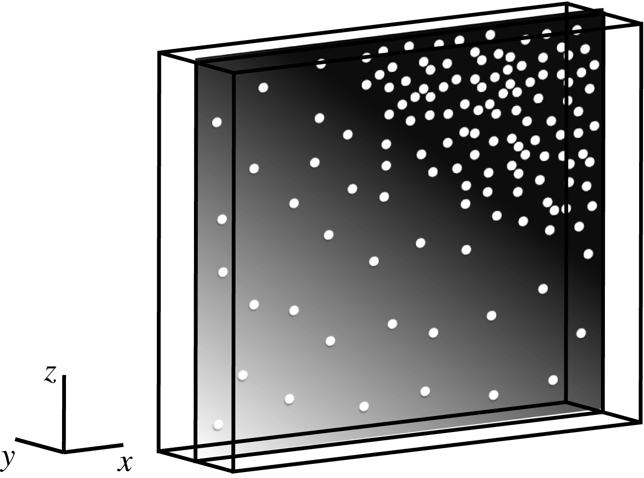
As base state, we consider a stably stratified incompressible Newtonian fluid at rest in a vertical Hele-Shaw cell, as shown in figure 1. The density of the fluid varies linearly in the vertical direction as a result of a stabilizing temperature gradient and a destabilizing sediment-concentration gradient. The sediment is characterized by a Stokes settling velocity and a constant diffusivity. We perform a linear stability analysis based on Darcy’s law, along with convection–diffusion equations for the temperature and sediment-concentration fields,
 $$\begin{eqnarray}\displaystyle & \boldsymbol{u}=-\unicode[STIX]{x1D735}p+Ra(T-C)\hat{\boldsymbol{k}}, & \displaystyle\end{eqnarray}$$
 $$\begin{eqnarray}\displaystyle & \displaystyle \frac{\unicode[STIX]{x2202}T}{\unicode[STIX]{x2202}t}+\boldsymbol{u}\boldsymbol{\cdot }\unicode[STIX]{x1D735}T=\unicode[STIX]{x1D6FB}^{2}T, & \displaystyle\end{eqnarray}$$
 $$\begin{eqnarray}\displaystyle & \displaystyle \frac{\unicode[STIX]{x2202}C}{\unicode[STIX]{x2202}t}+\boldsymbol{u}\boldsymbol{\cdot }\unicode[STIX]{x1D735}C-W_{st}\frac{\unicode[STIX]{x2202}C}{\unicode[STIX]{x2202}z}=\unicode[STIX]{x1D70F}\unicode[STIX]{x1D6FB}^{2}C, & \displaystyle\end{eqnarray}$$
 $$\begin{eqnarray}\displaystyle & \unicode[STIX]{x1D735}\boldsymbol{\cdot }\boldsymbol{u}=0. & \displaystyle\end{eqnarray}$$
In the above dimensionless equations,
 $\boldsymbol{u}=(u,w)$
indicates the gap-averaged fluid velocity,
 $p$
is the pressure,
 $\hat{\boldsymbol{k}}$
denotes the unit vector in the direction of gravity, and
 $T$
and
 $C$
represent the temperature and sediment-concentration fields respectively. Here, we assume that the density
 $\unicode[STIX]{x1D70C}$
depends linearly on
 $T$
and
 $C$
 $$\begin{eqnarray}\unicode[STIX]{x1D70C}=1-\unicode[STIX]{x1D6FC}(T-T_{m})+\unicode[STIX]{x1D6FD}(C-C_{m}),\end{eqnarray}$$
where
 $T_{m}$
and
 $C_{m}$
denote reference values, while
 $\unicode[STIX]{x1D6FC}$
and
 $\unicode[STIX]{x1D6FD}$
indicate constant expansion coefficients.
Schematic representation of a two-component stratified fluid in a vertical Hele-Shaw cell. Darker shading indicates higher temperature, and white dots represent settling particles.

The governing equations and the base state give rise to five dimensionless parameters,
 $$\begin{eqnarray}Ra=\frac{\unicode[STIX]{x1D6FC}b^{4}T_{0z}\unicode[STIX]{x1D70C}_{m}g}{12\unicode[STIX]{x1D707}\unicode[STIX]{x1D705}_{T}},\quad \unicode[STIX]{x1D70F}=\frac{\unicode[STIX]{x1D705}_{c}}{\unicode[STIX]{x1D705}_{T}},\quad W_{st}=\frac{W_{st}^{\ast }b}{\unicode[STIX]{x1D705}_{T}},\quad R_{\unicode[STIX]{x1D70C}}=\frac{\unicode[STIX]{x1D6FC}T_{0z}}{\unicode[STIX]{x1D6FD}C_{0z}},\quad \unicode[STIX]{x1D719}=\frac{T_{0x}}{T_{0z}}.\end{eqnarray}$$
These are obtained by introducing characteristic scales for length, time, velocity, temperature and sediment concentration respectively, in the form
 $[d]=b$
,
 $[t]=b^{2}/\unicode[STIX]{x1D705}_{T}$
,
 $[v]=\unicode[STIX]{x1D705}_{T}/b$
,
 $[T]=T_{0z}b$
and
 $[C]=\unicode[STIX]{x1D6FC}T_{0z}b/\unicode[STIX]{x1D6FD}$
. Here,
 $b$
denotes the gap width of the Hele-Shaw cell, while
 $\unicode[STIX]{x1D705}_{T}$
and
 $\unicode[STIX]{x1D705}_{C}$
indicate the thermal and sediment diffusivities respectively. The parameter
 $Ra$
represents a thermal Rayleigh number, which can be interpreted as the ratio of the pressure gradient due to the base state temperature gradient,
 $\unicode[STIX]{x1D6FC}T_{0z}b\unicode[STIX]{x1D70C}_{m}g$
, and a flow-induced pressure gradient,
 $12\unicode[STIX]{x1D707}\unicode[STIX]{x1D705}_{T}/b^{3}$
. The parameter
 $\unicode[STIX]{x1D70F}$
indicates the diffusivity ratio, and
 $W_{st}$
represents the Stokes settling velocity. The density ratio
 $R_{\unicode[STIX]{x1D70C}}$
arises from the base state profiles for the temperature and sediment concentration,
 $T_{0}$
and
 $C_{0}$
. The parameter
 $\unicode[STIX]{x1D719}$
accounts for linear horizontal gradients in the base state temperature and sediment-concentration profiles, which are assumed to be density-compensating, so that
 $\unicode[STIX]{x1D6FC}T_{0x}=\unicode[STIX]{x1D6FD}C_{0x}$
,
 $$\begin{eqnarray}T_{0}(x,z)=\unicode[STIX]{x1D719}x+z;\quad C_{0}(x,z,t)=\unicode[STIX]{x1D719}x+\frac{1}{R_{\unicode[STIX]{x1D70C}}}(z+W_{st}t).\end{eqnarray}$$
Realistic values of the governing parameters can be estimated along the following lines. The thermal diffusivity of water at room temperature is
 $\unicode[STIX]{x1D705}_{T}=0.145\times 10^{-6}~\text{m}^{2}~\text{s}^{-1}$
, the thermal expansion coefficient can be taken as
 $\unicode[STIX]{x1D6FC}=2\times 10^{-4}~\text{K}^{-1}$
, and
 $T_{0z}$
, in
 $^{\circ }\text{C}~\text{m}^{-1}$
, can range from
 $O(10^{-2})$
to
 $O(1)$
. In fact, in vertical fissures created by hydraulic fracturing, temperature gradients can change drastically, and variations between
 $T_{0z}=-0.8\,^{\circ }\text{C}~\text{m}^{-1}$
and
 $T_{0z}=2.7\,^{\circ }\text{C}~\text{m}^{-1}$
have been recorded (Dobkins Reference Dobkins1981). Following Reali et al. (Reference Reali, Garaud, Alsinan and Meiburg2017), the settling velocity can be estimated as
 $W_{st}=(b/\unicode[STIX]{x1D705}_{T})W_{st}^{\ast }=(b/\unicode[STIX]{x1D705}_{T})((2r^{2}(\unicode[STIX]{x1D70C}_{p}-\unicode[STIX]{x1D70C}_{m})g)/9\unicode[STIX]{x1D707})$
, where
 $r$
denotes the particle radius. The reference density,
 $\unicode[STIX]{x1D70C}_{m}$
, can vary from
 $800~\text{kg}~\text{m}^{-3}$
to
 $1200~\text{kg}~\text{m}^{-3}$
, spanning different materials such as oils, water and glycerin. On the other hand,
 $\unicode[STIX]{x1D70C}_{p}$
may range from
 $1200~\text{kg}~\text{m}^{-3}$
to
 $3900~\text{kg}~\text{m}^{-3}$
. It may represent the density of sediments, such as sand or clay, or of proppants used in hydraulic fracturing operations. These can comprise a variety of materials such as walnut shells, plastic, hollow glass, silica sand, resin-coated sand, ceramics and sintered bauxite (Liang et al.
Reference Liang, Sayed, Al-Munstasheri, Chang and Li2016). The dynamic viscosity can range from
 $\unicode[STIX]{x1D707}=1~\text{mPa}~\text{s}$
to
 $\unicode[STIX]{x1D707}=1000~\text{mPa}~\text{s}$
for oils or water–glycerin stable solutions. Based on these values, and considering gap sizes between 0.1 and 1 mm, the dimensionless settling velocity can be estimated as a function of the particle radius,
 $r$
. It can range from values as low as
 $W_{st}\approx 10^{-10}$
to as high as
 $W_{st}\approx 500$
for particle sizes from colloidal size to hundreds of microns. This provides the motivation for analysing the influence of this parameter across several orders of magnitude.
The diffusivity ratio can be estimated as in Reali et al. (Reference Reali, Garaud, Alsinan and Meiburg2017), from the sum of two contributions: Brownian motion and hydrodynamic diffusion of the individual grains due to their long-range interactions, which yields
 $\unicode[STIX]{x1D70F}=\unicode[STIX]{x1D705}_{c}/\unicode[STIX]{x1D705}_{T}=k_{B}T_{m}/6\unicode[STIX]{x03C0}\unicode[STIX]{x1D707}r\unicode[STIX]{x1D705}_{T}+(r/b)W_{st}$
. The first term dominates for submicron particles, while the second term becomes important for larger sediment grains. Using the above estimates, the Rayleigh number
 $Ra$
can be calculated to range from
 $7.2\times 10^{-11}$
to
 $3.7\times 10^{-3}$
.
3 Linear stability analysis
By decomposing the velocity, temperature and sediment-concentration fields into base states and perturbations, we can linearize (2.1)–(2.4) to obtain
 $$\begin{eqnarray}\displaystyle & \displaystyle u+\frac{\unicode[STIX]{x2202}p}{\unicode[STIX]{x2202}x}=0,\quad w+\frac{\unicode[STIX]{x2202}p}{\unicode[STIX]{x2202}z}-Ra(T-C)=0, & \displaystyle\end{eqnarray}$$
 $$\begin{eqnarray}\displaystyle & \displaystyle \frac{\unicode[STIX]{x2202}T}{\unicode[STIX]{x2202}t}+\unicode[STIX]{x1D719}u+w-\unicode[STIX]{x1D6FB}^{2}T=0, & \displaystyle\end{eqnarray}$$
 $$\begin{eqnarray}\displaystyle & \displaystyle \frac{\unicode[STIX]{x2202}C}{\unicode[STIX]{x2202}t}+\unicode[STIX]{x1D719}u+\frac{1}{R_{\unicode[STIX]{x1D70C}}}w-W_{st}\frac{\unicode[STIX]{x2202}C}{\unicode[STIX]{x2202}z}-\unicode[STIX]{x1D70F}\unicode[STIX]{x1D6FB}^{2}C=0, & \displaystyle\end{eqnarray}$$
 $$\begin{eqnarray}\displaystyle & \displaystyle \frac{\unicode[STIX]{x2202}u}{\unicode[STIX]{x2202}x}+\frac{\unicode[STIX]{x2202}w}{\unicode[STIX]{x2202}z}=0. & \displaystyle\end{eqnarray}$$
Elimination of the pressure by introducion of the vorticity variable yields
 $$\begin{eqnarray}\unicode[STIX]{x1D6FA}-Ra\frac{\unicode[STIX]{x2202}}{\unicode[STIX]{x2202}x}(T-C)=0,\quad \unicode[STIX]{x1D6FA}=\frac{\unicode[STIX]{x2202}w}{\unicode[STIX]{x2202}x}-\frac{\unicode[STIX]{x2202}u}{\unicode[STIX]{x2202}z},\end{eqnarray}$$
which demonstrates that the presence of vorticity is associated with horizontal temperature and sediment-concentration gradients.
The employment of normal modes
 $(u,w,T,C)\sim \text{Re}[(\hat{u} ,{\hat{w}},\hat{T},{\hat{C}})\exp (\unicode[STIX]{x1D706}t+\text{i}lx+\text{i}kz)]$
allows us to rewrite (3.2)–(3.5) in terms of the eigenfunctions
 $(\hat{u} ,{\hat{w}},\hat{T},{\hat{C}})$
and the vertical and horizontal real wavenumbers
 $(k,l)$
to obtain a quadratic equation for the complex growth rate
 $\unicode[STIX]{x1D706}$
, where
 $K^{2}=k^{2}+l^{2}$
,
 $$\begin{eqnarray}\displaystyle & \unicode[STIX]{x1D706}^{2}+a_{1}\unicode[STIX]{x1D706}+a_{2}=0, & \displaystyle\end{eqnarray}$$
 $$\begin{eqnarray}\displaystyle & \displaystyle a_{1}=K^{2}(1+\unicode[STIX]{x1D70F})+\frac{Ra\,l^{2}}{K^{2}}\left(1-\frac{1}{R_{\unicode[STIX]{x1D70C}}}\right)-\text{i}kW_{st}, & \displaystyle\end{eqnarray}$$
 $$\begin{eqnarray}\displaystyle & \displaystyle a_{2}=\unicode[STIX]{x1D70F}K^{4}+Ra\,l^{2}\left(\unicode[STIX]{x1D70F}-\frac{1}{R_{\unicode[STIX]{x1D70C}}}\right)+Ra\,l\unicode[STIX]{x1D719}k(1-\unicode[STIX]{x1D70F})-\text{i}kW_{st}\left[\frac{Ra\,l}{K^{2}}(l-\unicode[STIX]{x1D719}k)+K^{2}\right]\!. & \displaystyle\end{eqnarray}$$
We can relate this result to the linear stability analyses of Rudraiah et al. (Reference Rudraiah, Srimani and Friedrich1982) and Alsinan et al. (Reference Alsinan, Meiburg and Garaud2017). The former conducted an analysis of a two-component fluid in a saturated porous layer based on an extended version of Darcy’s law that included inertial effects, while the latter considered the Navier–Stokes equations in stratified fluids. Both analyses yielded cubic polynomials for the growth rate, which reduce to quadratic forms if the inertial terms in the momentum equation are neglected, or in the limit of infinite Prandtl number. In addition, the current result reduces to that of Rudraiah et al. (Reference Rudraiah, Srimani and Friedrich1982) when
 $\unicode[STIX]{x1D719}=0$
and
 $W_{st}=0$
. The above quadratic expression enables us to obtain exact forms of the neutral stability curves and to investigate limiting behaviours.
For the general case in which
 $W_{st}\neq 0$
, an implicit relationship for the neutral stability curve can be obtained by setting the real part of the growth rate to zero,
 $\unicode[STIX]{x1D706}_{R}=0$
. This criterion can be obtained by combining the roots of the quadratic equation (3.6) with an explicit representation of the square root of a complex number, i.e. by simplifying
 $\text{Re}(\sqrt{\unicode[STIX]{x1D6E5}})=(1/\sqrt{2})[(\text{Re}(\unicode[STIX]{x1D6E5})^{2}+\text{Im}(\unicode[STIX]{x1D6E5})^{2})^{1/2}+\text{Re}(\unicode[STIX]{x1D6E5})]^{1/2}=\text{Re}(a_{2})$
, where
 $\unicode[STIX]{x1D6E5}=a_{1}^{2}-4a_{2}$
,
 $$\begin{eqnarray}\displaystyle & & \displaystyle W_{st}^{2}k^{2}\left[K^{2}(\unicode[STIX]{x1D70F}-1)+\frac{Ra\,l^{2}}{K^{2}}\left(2\frac{k}{l}\unicode[STIX]{x1D719}-1-\frac{1}{R_{\unicode[STIX]{x1D70C}}}\right)\right]^{2}=\left[K^{2}(1+\unicode[STIX]{x1D70F})+\frac{Ra\,l^{2}}{K^{2}}\left(1-\frac{1}{R_{\unicode[STIX]{x1D70C}}}\right)\right]^{2}\nonumber\\ \displaystyle & & \displaystyle \quad \times \left[4\unicode[STIX]{x1D70F}K^{4}+4\,Ra\,l^{2}\left(\unicode[STIX]{x1D70F}-\frac{1}{R_{\unicode[STIX]{x1D70C}}}\right)+4\,Ra\,l\unicode[STIX]{x1D719}k(1-\unicode[STIX]{x1D70F})+W_{st}^{2}k^{2}\right]\!.\end{eqnarray}$$
In the following, we use the above equations to investigate how the dimensionless governing parameters influence the onset of double-diffusive and settling-driven instabilities.
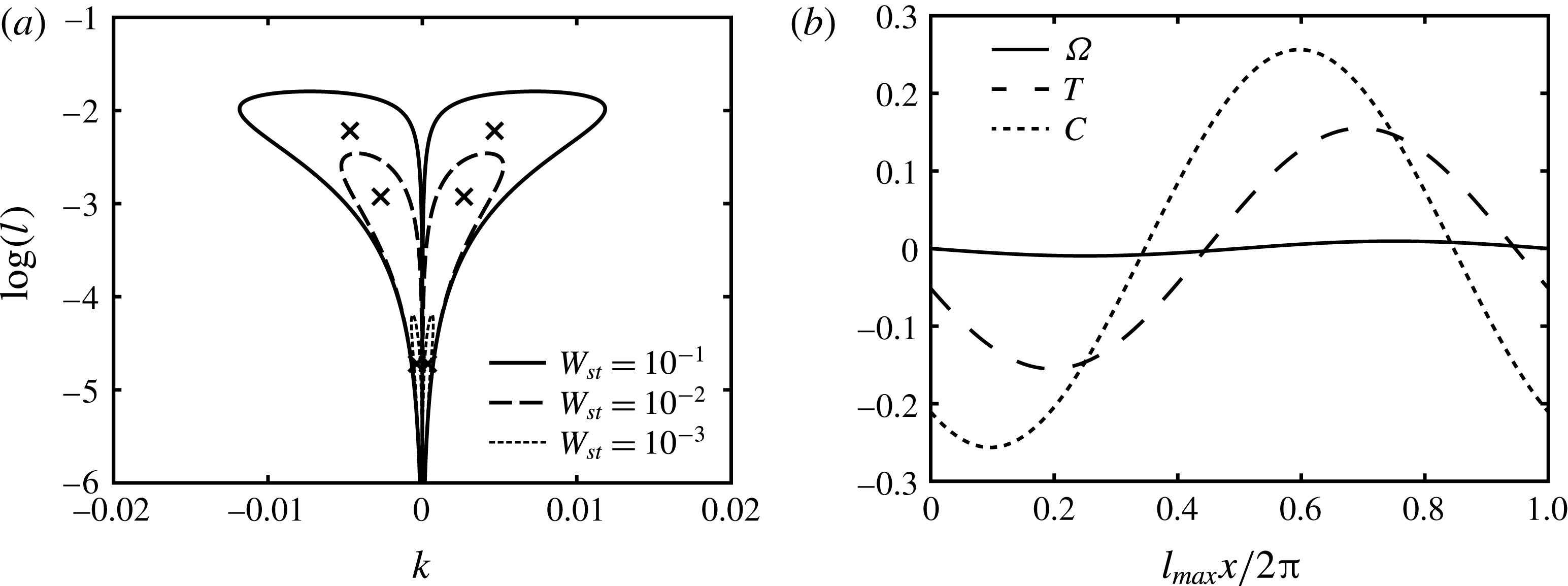
For
 $(Ra,\unicode[STIX]{x1D70F},R_{\unicode[STIX]{x1D70C}},\unicode[STIX]{x1D719})=(10^{-3},1,1.5,0)$
. (a) Neutral stability curve,
 $\unicode[STIX]{x1D706}_{R}=0$
, as a function of the vertical and horizontal wavenumbers
 $k$
and
 $l$
, for different values of
 $W_{st}$
. Pairs of wavenumbers
 $(\pm k,l)$
bounded by these contours have positive real parts of the growth rate,
 $\unicode[STIX]{x1D706}_{R}$
, and their corresponding maximum values are marked with an ‘
 $\times$
’. (b) Horizontal cross-sections,
 $z=0$
, of the normalized eigenfunctions,
 $\unicode[STIX]{x1D6FA}$
,
 $T$
and
 $C$
for
 $W_{st}=10^{-1}$
. For visualization purposes, the amplitudes of the
 $T$
and
 $C$
eigenfunctions are multiplied by
 $10^{-4}$
. The settling velocity creates a phase shift between the temperature and sediment-concentration perturbations. This corresponds to a phase shift between stabilizing
 $T$
and destabilizing
 $C$
waves that drives unstable growth.

3.1 Settling-driven instability
We begin by considering the case
 $\unicode[STIX]{x1D70F}=1$
, so that temperature and sediment diffuse at the same rate and double-diffusive instabilities are absent. In addition, we eliminate horizontal base state gradients by setting
 $\unicode[STIX]{x1D719}=0$
. In this configuration, the only potentially destabilizing mechanism is provided by the settling velocity. The corresponding Navier–Stokes situation was investigated by Alsinan et al. (Reference Alsinan, Meiburg and Garaud2017), who found that the settling velocity creates a destabilizing phase shift between the
 $T$
and
 $C$
perturbations. We observe a similar behaviour in the current Darcy environment, which again triggers the growth of inclined waves.
Figure 2(a) shows the neutral stability curve,
 $\unicode[STIX]{x1D706}_{R}=0$
, as a function of the vertical and horizontal wavenumbers
 $k$
and
 $l$
, for different values of the settling velocity
 $W_{st}$
and
 $(Ra,\unicode[STIX]{x1D70F},R_{\unicode[STIX]{x1D70C}},\unicode[STIX]{x1D719})=(10^{-3},1,1.5,0)$
. Positive
 $\unicode[STIX]{x1D706}_{R}$
values are found inside these contours, and the fastest growing modes are marked by an ‘
 $\times$
’. Symmetry across the
 $k=0$
line reflects the inclined nature of the settling-driven unstable waves. The phase shift between the
 $T$
and
 $C$
waves responsible for instability growth is shown in the horizontal cross-sections of the normalized eigenfunctions of
 $\unicode[STIX]{x1D6FA}$
,
 $T$
and
 $C$
in figure 2(b).
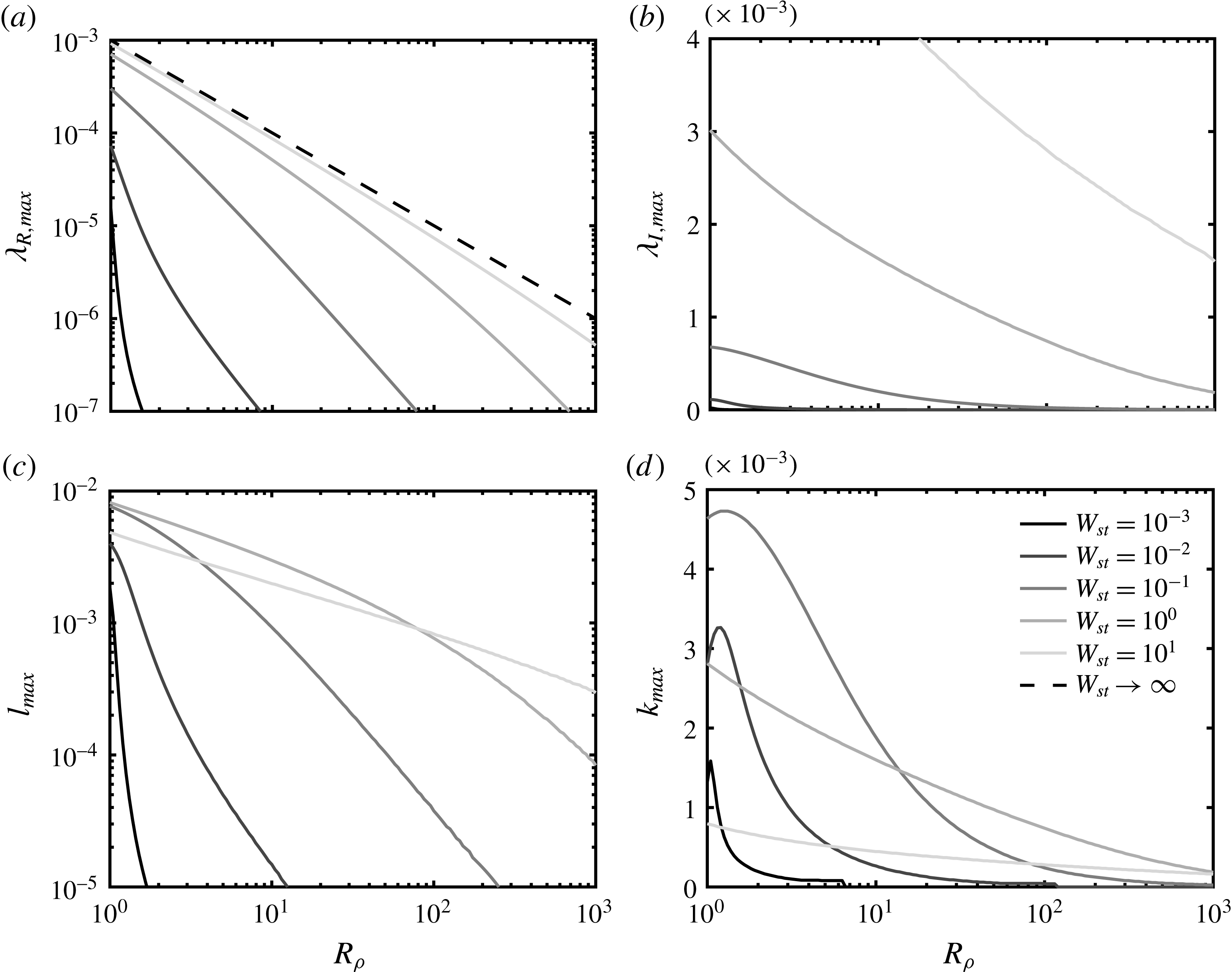
Properties of the fastest growing mode as a function of the density ratio
 $R_{\unicode[STIX]{x1D70C}}$
for a wide range of
 $W_{st}$
and
 $(Ra,\unicode[STIX]{x1D70F},\unicode[STIX]{x1D719})=(10^{-3},1,0)$
. Temperature and sediment diffuse at the same rate, so that the instability is purely settling-driven. (a) Real part of the maximum growth rate,
 $\unicode[STIX]{x1D706}_{R,max}$
, for different
 $W_{st}$
values, for large settling velocities,
 $\unicode[STIX]{x1D706}_{R,max}\sim R_{\unicode[STIX]{x1D70C}}^{-1}$
. (b) The imaginary part
 $\unicode[STIX]{x1D706}_{I,max}$
of the fastest growing mode, indicative of the wave velocity, increases with
 $W_{st}$
. (c) The horizontal wavenumber of the fastest growing mode decreases with
 $R_{\unicode[STIX]{x1D70C}}$
and increases with
 $W_{st}$
, until it peaks near
 $W_{st}\approx 0.35$
. (d) The dominant vertical wavenumber increases with
 $W_{st}$
up to
 $W_{st}\approx 0.11$
.

The dependence of the growth rate and wavenumbers of the settling-driven instability on the density ratio is shown in figure 3. For constant
 $W_{st}$
,
 $\unicode[STIX]{x1D706}_{R,max}$
decreases with increasing
 $R_{\unicode[STIX]{x1D70C}}$
, since the overall density gradient becomes more stable. For large settling velocities,
 $\unicode[STIX]{x1D706}_{R,max}\sim R_{\unicode[STIX]{x1D70C}}^{-1}$
, cf. figure 3(a), as
 $\unicode[STIX]{x1D706}_{R}$
approaches the limiting behaviour,
 $$\begin{eqnarray}\unicode[STIX]{x1D706}_{R}(W_{st}\rightarrow \infty )=\frac{Ra\,l}{K^{2}}\left(\frac{l}{R_{\unicode[STIX]{x1D70C}}}-k\unicode[STIX]{x1D719}\right)-\unicode[STIX]{x1D70F}K^{2}.\end{eqnarray}$$
The imaginary part of the growth rate shown in figure 3(b) increases monotonically with the settling velocity, indicating a growing phase shift between
 $T$
and
 $C$
waves. Figures 3(c) and 3(d), however, indicate that both the horizontal and the vertical wavenumbers reach maxima at moderate
 $W_{st}$
values.
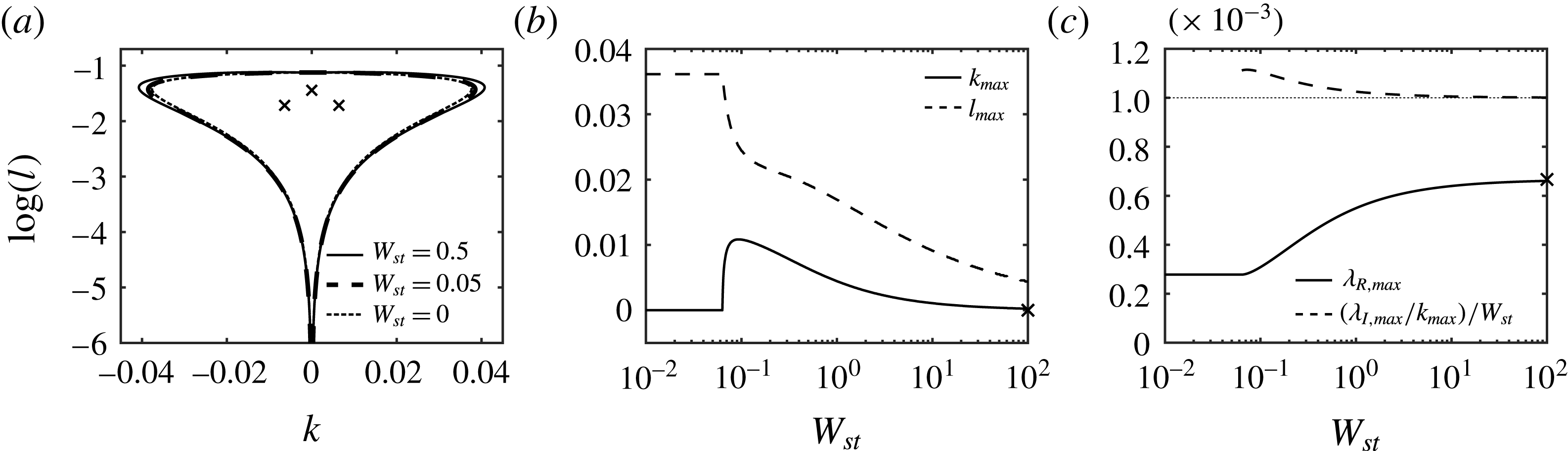
For
 $(Ra,\unicode[STIX]{x1D70F},R_{\unicode[STIX]{x1D70C}},\unicode[STIX]{x1D719})=(10^{-3},0.1,1.5,0)$
. (a) Neutral stability curve as function of
 $k$
and
 $l$
, for different
 $W_{st}$
values. Positive growth rates exist within the contours. For both
 $W_{st}=0$
and
 $W_{st}=0.05$
, only the double-diffusive instability is active, and the elevator mode
 $k=0$
is most amplified. Beyond a critical
 $W_{st}$
value, the settling-driven mode becomes dominant, so that the fastest growing waves are inclined. (b) Fastest growing vertical
 $(k_{max})$
and horizontal
 $(l_{max})$
wavenumbers as functions of
 $W_{st}$
. Beyond a critical value of the particle settling velocity,
 $W_{st,crit}\approx 0.06$
, the dominant instability mode changes from
 $k=0$
to inclined waves. The symbols indicate limiting values as
 $W_{st}\rightarrow \infty$
. (c) The most unstable growth rate and the normalized vertical phase velocity as functions of
 $W_{st}$
. Here,
 $\unicode[STIX]{x1D706}_{R,max}$
monotonically increases beyond
 $W_{st,crit}$
and asymptotically approaches
 $\unicode[STIX]{x1D706}_{R}=(2/3)\times 10^{-3}$
. The vertical phase velocity approaches the particle settling velocity for large
 $W_{st}$
values. For visualization purposes, the values of
 $\unicode[STIX]{x1D706}_{I,max}$
are multiplied by
 $10^{-3}$
.

We proceed to the case of
 $\unicode[STIX]{x1D70F}=0.1$
, for which the thermal diffusivity is larger than the sediment diffusivity. Now, both double-diffusive and settling-driven instabilities are present, so that we can investigate their interaction. Figure 4(a) shows the neutral stability curve as a function of the vertical and horizontal wavenumbers for increasing
 $W_{st}$
values. Positive growth rates are found within the contours. For both
 $W_{st}=0$
and
 $W_{st}=0.05$
, the maximum growth rate corresponds to the elevator mode
 $k=0$
, as indicated by two overlapping ‘
 $\times$
’ symbols. For
 $W_{st}=0.5$
, the settling-driven instability mode dominates, giving rise to inclined waves.
Figure 4(b) shows the fastest growing vertical and horizontal wavenumbers as functions of
 $W_{st}$
. Beyond a critical value of the settling velocity,
 $W_{st,crit}\approx 0.06$
, the settling-driven instability mode dominates, marking the transition from elevator mode to inclined waves. Consequently,
 $k_{max}$
increases beyond
 $W_{st,crit}$
, peaks near
 $W_{st,peak}\approx 0.09$
and subsequently decreases, asymptotically approaching zero as
 $W_{st}\rightarrow \infty$
, as indicated by the symbol ‘
 $\times$
’. Beyond
 $W_{st,crit}$
,
 $l_{max}$
decreases monotonically, indicating a shift to longer waves as
 $W_{st}$
increases. Figure 4(c) shows the maximum value of the real part of the growth rate, along with the normalized vertical phase velocity, as functions of
 $W_{st}$
. Beyond
 $W_{st,crit}$
,
 $\unicode[STIX]{x1D706}_{R,max}$
increases monotonically, and it asymptotically approaches
 $\unicode[STIX]{x1D706}_{R}=Ra(1/R_{\unicode[STIX]{x1D70C}}-\unicode[STIX]{x1D719})=(2/3)\times 10^{-3}$
for
 $W_{st}\rightarrow \infty$
,
 $k_{max}\rightarrow 0$
and
 $l_{max}\rightarrow 0$
. The vertical phase velocity asymptotically approaches the particle settling velocity for large
 $W_{st}$
.
3.2 Influence of lateral gradients
In figure 5, we analyse how lateral base state gradients modify the case
 $(Ra,\unicode[STIX]{x1D70F},R_{\unicode[STIX]{x1D70C}},W_{st})=(10^{-3},1,1.5,10^{-2})$
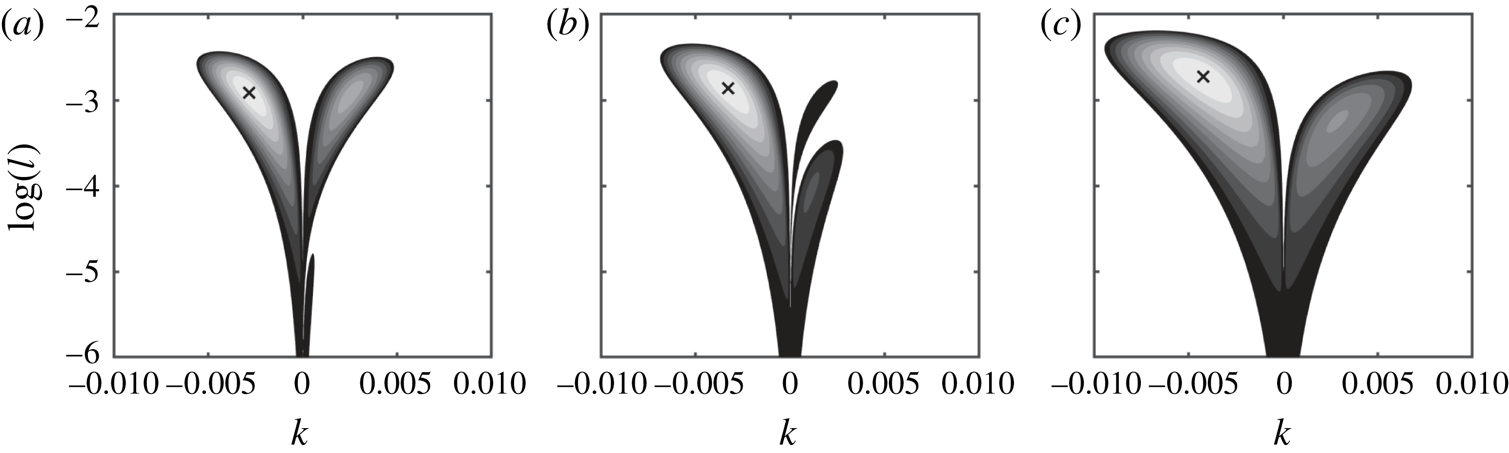
, which we had investigated in figure 2(a). Figure 5(a) clearly demonstrates how the symmetry of the two lobes is broken for
 $\unicode[STIX]{x1D719}=0.04$
. A new intrusive instability mode is observed for small
 $k$
values, similar to the situation in Navier–Stokes flows (Ruddick & Richards Reference Ruddick and Richards2003; Medrano, Garaud & Stellmach Reference Medrano, Garaud and Stellmach2014). This intrusive instability mode possesses smaller wavenumbers than the waves of the dominant settling-driven instability branch and triggers the growth of waves that are inclined opposite to them. For
 $\unicode[STIX]{x1D719}=0.2$
, figure 5(b), the intrusive lobe further increases in area and magnitude, while the settling-driven lobe with
 $k>0$
shrinks. At
 $\unicode[STIX]{x1D719}=0.7$
, figure 5(c), only the intrusive lobe remains for
 $k>0$
.
The positive real part of the growth rate as a function of the vertical,
 $k$
, and horizontal,
 $l$
, wavenumbers for
 $(Ra,\unicode[STIX]{x1D70F},R_{\unicode[STIX]{x1D70C}},W_{st})=(10^{-3},1,1.5,10^{-2})$
and (a)
 $\unicode[STIX]{x1D719}=0.04$
, (b)
 $\unicode[STIX]{x1D719}=0.2$
, (c)
 $\unicode[STIX]{x1D719}=0.7$
. The most amplified mode is marked with an ‘
 $\times$
’. Double-diffusive instabilities are absent and lateral base state gradients break the symmetry of the system, triggering a new intrusive instability mode.

We now proceed to analyse how the fastest growing mode changes with the strength of the double-diffusive instability, the lateral gradients and the settling velocity, and discuss stability criteria. Whenever instability growth happens, driven by double diffusion, settling or a combination of these effects, a neutral stability curve will exist in the form of a bounded region in the
 $(l,k)$
space, with the fastest growing modes lying inside the closed neutral stability curve. An example is the instability purely driven by settling discussed in figure 2(a), where instability is found for
 $W_{st}>0$
and smaller positive
 $W_{st}$
values reduce both the area of the neutral stability curve and the magnitude of the dominant modes. As a result, the existence of a neutral stability curve guarantees the existence of a dominant mode, and instability criteria for the dominant modes can be interpreted on the basis of the neutral stability relationships of (3.6).
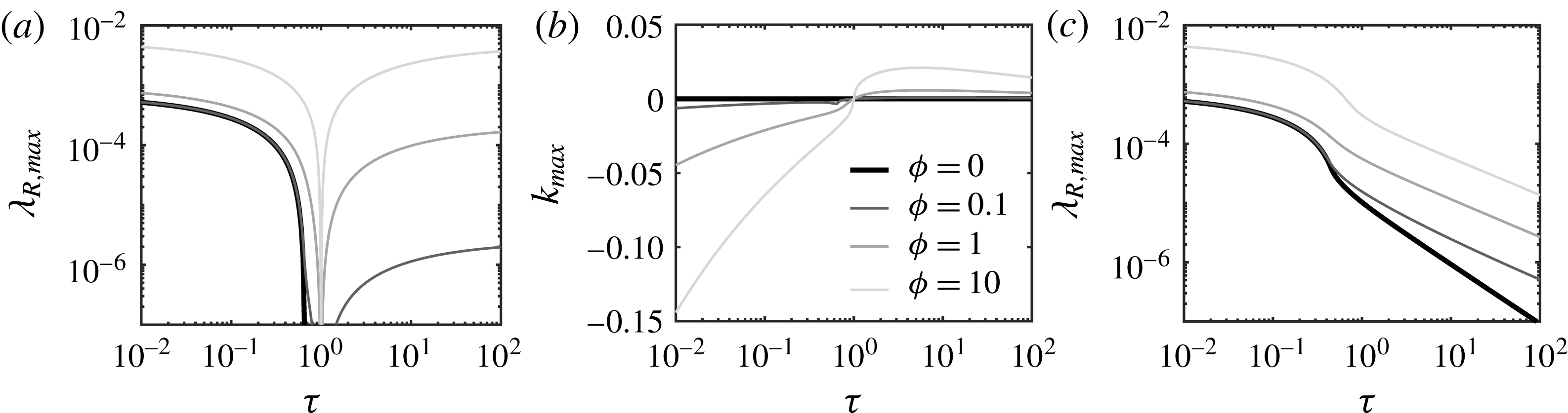
(a) The maximum real part of the growth rate,
 $\unicode[STIX]{x1D706}_{R,max}$
, and (b) the maximum vertical wavenumber,
 $k_{max}$
, as functions of the diffusivity ratio
 $\unicode[STIX]{x1D70F}$
for
 $W_{st}=0$
. (c) The maximum real part of the growth rate,
 $\unicode[STIX]{x1D706}_{R,max}$
, for
 $W_{st}=10^{-2}$
. The remaining parameters are
 $(Ra,R_{\unicode[STIX]{x1D70C}})=(10^{-3},1.5)$
.

For
 $W_{st}=0$
, figure 6(a) shows the maximum real part of the growth rate,
 $\unicode[STIX]{x1D706}_{R,max}$
, and figure 6(b) the maximum vertical wavenumber,
 $k_{max}$
, as functions of the diffusivity ratio,
 $\unicode[STIX]{x1D70F}$
, for different values of the lateral base state gradients. Figure 6(c) indicates the corresponding
 $\unicode[STIX]{x1D706}_{R,max}$
for
 $W_{st}=10^{-2}$
. For
 $W_{st}=0$
, the growth rate is real and the neutral stability curve can be obtained by setting the coefficient
 $a_{2}=0$
. This leads to
 $$\begin{eqnarray}\unicode[STIX]{x1D70F}K^{4}=Ra\,l^{2}\left(\frac{1}{R_{\unicode[STIX]{x1D70C}}}-\unicode[STIX]{x1D70F}\right)+Ra\,l\unicode[STIX]{x1D719}k(\unicode[STIX]{x1D70F}-1)>0.\end{eqnarray}$$
It should be noticed that if
 $\unicode[STIX]{x1D719}=0$
, the above equation is satisfied when
 $\unicode[STIX]{x1D70F}<1/R_{\unicode[STIX]{x1D70C}}$
. This instability criterion is consistent with previous experiments and linear stability results; cf. Cooper et al. (Reference Cooper, Glass and Tyler1997). In the presence of lateral gradients
 $\unicode[STIX]{x1D719}>0$
, and since the last term in (3.11) is always positive because
 $k_{max}$
changes sign when
 $\unicode[STIX]{x1D70F}$
crosses 1, instability can be seen whenever
 $\unicode[STIX]{x1D70F}\neq 1$
. This behaviour of
 $k_{max}$
indicates that waves are inclined in opposite directions if the thermal diffusivity is different from the sediment diffusivity. When
 $\unicode[STIX]{x1D70F}=1$
, the above equation cannot be satisfied for
 $R_{\unicode[STIX]{x1D70C}}\geqslant 1$
, and the flow is stable regardless of the values of
 $\unicode[STIX]{x1D719}$
. This is expected since both double diffusion and settling velocity are absent. These results are consistent with the findings of Alsinan et al. (Reference Alsinan, Meiburg and Garaud2017) for double-diffusive and settling-driven instabilities in Navier–Stokes environments.
The situation for
 $W_{st}=1$
requires an analysis based on (3.9). Since many terms in this equation are squared, this equation can be satisfied whenever the last square bracket is non-negative, i.e.
 $$\begin{eqnarray}4\unicode[STIX]{x1D70F}K^{4}+W_{st}^{2}k^{2}\geqslant 4\,Ra\,l^{2}\left(\frac{1}{R_{\unicode[STIX]{x1D70C}}}-\unicode[STIX]{x1D70F}\right)+4\,Ra\,l\unicode[STIX]{x1D719}k(\unicode[STIX]{x1D70F}-1).\end{eqnarray}$$
This equation does not impose any restriction on the parameters, and it is satisfied even when the right-hand side becomes negative. Consistent with this observation, instability is found for all values of
 $\unicode[STIX]{x1D70F}$
and
 $\unicode[STIX]{x1D719}$
investigated; cf. figure 6(c).
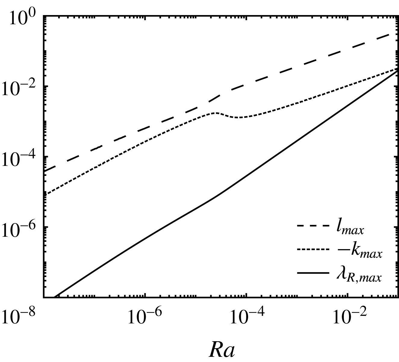
The maximum vertical,
 $-k_{max}$
, and horizontal,
 $l_{max}$
, wavenumbers and maximum real part of the growth rate,
 $\unicode[STIX]{x1D706}_{R,max}$
, for
 $(R_{\unicode[STIX]{x1D70C}},\unicode[STIX]{x1D70F},\unicode[STIX]{x1D719},W_{st})=(1.5,0.1,0.1,10^{-2})$
as functions of the Rayleigh number. The maximum growth rate is approximately proportional to
 $Ra$
.

Figure 7 shows how the maximum values of the real growth rate, along with the vertical and horizontal wavenumbers, change as a function of the Rayleigh number,
 $Ra$
. The presence of positive lateral gradients renders the dominant vertical wavenumber negative. As suggested by (3.5), the maximum growth rate is approximately proportional to
 $Ra$
. Larger wavenumbers grow faster as we increase vertical temperature gradients. This result is consistent with the stability criterion established by Nield (Reference Nield1968) for a fluid in an unbounded domain, where instability is expected for
 $Ra>0$
.
4 Conclusions
We have investigated the onset of instability in a stably stratified two-component fluid in a vertical Hele-Shaw cell, when the unstably stratified scalar has a settling velocity. Similarly to Navier–Stokes flows, this settling velocity triggers a new instability mode, which competes with the double-diffusive mode for unequal diffusivities. Below a critical value of
 $W_{st}$
, the double-diffusive elevator mode dominates, while, above this threshold, the inclined waves associated with the settling-driven instability exhibit faster growth. The analysis yields the neutral stability curves and allows for the discussion of various asymptotic limits. A natural extension of the current analysis will address the nonlinear evolution of these instabilities by means of direct numerical simulations.
Acknowledgement
The authors gratefully acknowledge financial support by NSF grant CBET-1438052.