2 Statement of the problem

Let us consider the unit square $E_{0}=\left[ 0,1\right] ^{2}$ . Let us divide $E_{0}$ into 9 equal subcubes of side $1/3$ . Let $\mathcal{SC}_{1}$ be the set of eight subsquares remaining after removing the interior of the central subsquare and let $E_{1}=\bigcup \left\{ C\text{; }C\in \mathcal{SC}_{1}\right\} $ . Repeating the process, subdividing each element of $\mathcal{SC}_{1}$ into 9 equal subcubes of side $1/9$ , we obtain $E_{2}=\bigcup\left\{ C\text{; }C\in \mathcal{SC}_{2}\right\} $ , where $\mathcal{SC}_{2}$ is the set of subcubes remaining after removing the interior of the central subsquare from each element of $\mathcal{SC}_{1}$ . 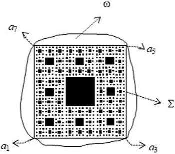Continuing in this way (see Figure 2), we obtain a decreasing sequence of compact sets $\left( E_{h}\right) _{h\in\mathbb{N}}$ . The set $\Sigma $ defined by

(2.1) \begin{equation}\Sigma =\underset{h=0}{\overset{\infty }{\bigcap }}E_{h}\text{,}\end{equation}

is the standard Sierpinski carpet. The set $\Sigma $ can be obtained as an iterated function system construction. Let $a_{1}=\left( 0,0\right) $ , $a_{2}=\left( 1/2,0\right) $ , $a_{3}=\left( 1,0\right) $ , $a_{4}=\left(1,1/2\right) $ , $a_{5}=\left( 1,1\right) $ , $a_{6}=\left( 1/2,1\right) $ , $a_{7}=\left( 0,1\right) $ , $a_{8}=\left( 0,1/2\right) $ . We suppose that

(2.2) \begin{equation}E_{0}\subset \overline{\omega }\text{ and }E_{0}\cap \partial \omega=\left\{ a_{1},a_{3},a_{5},a_{7}\right\} \text{,} \end{equation}

Figure 2.

The construction of Sierpinski carpet.

where $\omega $ is the bounded domain of $\mathbb{R}^{2}$ with Lipschitz continuous boundary $\partial \omega $ , which was already set in the Introduction. Let us denote by $\left\{ \psi _{i}\right\} _{i=1,...,8}$ the family of contractive similitudes defined on $\mathbb{R}^{2}$ by

(2.3) \begin{equation}\psi _{i}\left( x^{\prime }\right) =\frac{x^{\prime }+2a_{i}}{3}\text{, }\forall x^{\prime }=\left( x_{1},x_{2}\right) \in \mathbb{R}^{2}\text{.}\end{equation}

Then, $\Sigma $ is the unique non-empty compact set of $\mathbb{R}^{2}$ satisfying

(2.4) \begin{equation}\Sigma =\underset{i=1}{\overset{8}{\bigcup }}\psi _{i}\left( \Sigma \right)\text{.} \end{equation}

Let us set $\mathcal{V}_{0}=\left\{a_{1},a_{2},a_{3},a_{4},a_{5},a_{6},a_{7},a_{8}\right\} $ . Let $h\in \mathbb{N}^{\ast }$ . We consider the set of vertices $\mathcal{V}_{i_{1}...i_{h}}$ ; $i_{1},...,i_{h}\in \left\{ 1,...,8\right\} $ , defined by

(2.5) \begin{equation}\mathcal{V}_{i_{1}...i_{h}}=\psi _{i_{1}}\circ ...\circ \psi _{i_{h}}\left(\mathcal{V}_{0}\right) \text{.} \end{equation}

We then set

(2.6) \begin{equation}\mathcal{V}_{h}=\left\{\begin{array}{ll}\mathcal{V}_{0} & \text{for }h=0\text{,} \\ \underset{i_{1},...,i_{h}\in \left\{ 1,...,8\right\} }{\bigcup }\mathcal{V}_{i_{1}...i_{h}} & \text{for }h\in \mathbb{N}^{\ast }\end{array}\right. \end{equation}

and

(2.7) \begin{equation}\mathcal{V}_{\infty }=\underset{h\in \mathbb{N}}{\bigcup }\mathcal{V}_{h}\text{.} \end{equation}

We consider the connected graph $\Sigma _{i_{1}...i_{h}}=\left( \mathcal{V}_{i_{1}...i_{h}},S_{i_{1}...i_{h}}\right) $ , where $S_{i_{1}...i_{h}}$ is the set of edges $\left[ p,q\right] $ with $p,q\in \mathcal{V}_{i_{1}...i_{h}}$ , such that $\left\vert p-q\right\vert =3^{-h}/2$ ; $\left\vert p-q\right\vert $ being the Euclidian distance between p and q. We denote by $S_{0}$ the set of edges $\left[ p,q\right] $ with $p,q\in\mathcal{V}_{0}$ , such that $\left\vert p-q\right\vert =1/2$ , $\Sigma_{0}=\left( \mathcal{V}_{0},S_{0}\right) $ , and set

(2.8) \begin{equation}\left\{\begin{array}{ccc}S_{h} & = & \underset{i_{1},...,i_{h}\in \left\{ 1,...,8\right\} }{\bigcup }S_{i_{1}...i_{h}}\text{, }\forall h\in \mathbb{N}^{\ast }\text{,} \\& & \\\Sigma _{h} & = & \underset{i_{1},...,i_{h}\in \left\{ 1,...,8\right\} }{\bigcup }\Sigma _{i_{1}...i_{h}}\text{, }\forall h\in \mathbb{N}^{\ast }\text{.}\end{array}\right. \end{equation}

We also define

(2.9) \begin{equation}\left\{\begin{array}{lll}S_{h}^{1} & = & \underset{\left[ p,q\right] \subset S_{h}\text{: }\left[ p,q\right] \perp \left( 0,1\right) }{\bigcup }\left[ p,q\right] \text{,} \\& & \\S_{h}^{2} & = & \underset{\left[ p,q\right] \subset S_{h}\text{: }\left[ p,q\right] \perp \left( 1,0\right) }{\bigcup }\left[ p,q\right] \text{,}\end{array}\right. \end{equation}

where $\left[ p,q\right] \perp \left( 0,1\right) $ (resp. $\left[ p,q\right]\perp \left( 1,0\right) $ ) means that the line segment $\left[ p,q\right] $ is perpendicular to the unit vector $\left( 0,1\right) $ (resp. $\left(1,0\right) $ ).

Let $N_{h}^{v}$ be the number of vertices in $\mathcal{V}_{h}$ and let $N_{h}^{e}$ be the number of edges in $S_{h}$ . These numbers can be computed by using the proof of [Reference Malo30, Lemma 2.1.2]. Indeed, $N_{h}^{v}$ can be obtained by adding the number of midpoints of the edges of the graph approximation of the Sierpinski carpet of [Reference Malo30, Paragraph 2.1] to the number of vertices obtained in [Reference Malo30, Lemma 2.1.2], then, using the proof of [Reference Malo30, Lemma 2.1.2], $N_{h}^{e}$ can be obtained by induction. We have, for $h\geq 2$ ,

(2.10) \begin{equation}\begin{array}{lll}N_{h}^{v} & = & \left( 3^{h+1}+1\right) \left( 3^{h}+1\right) -\underset{k=0}{\overset{h-2}{\sum }}8^{k}\left( 3^{h-1-k}-1\right) \left( 3^{h-k}-1\right)\text{,} \\ N_{h}^{e} & = & 4\left( 3^{h}\left( 3^{h}+1\right) -\underset{k=0}{\overset{h-2}{\sum }}8^{k}3^{h-1-k}\left( 3^{h-1-k}-1\right) \right) \text{,}\end{array}\end{equation}

from which we deduce, by a straightforward computation, that

(2.11) \begin{equation}\begin{array}{rrr}N_{h}^{v} & \underset{h\rightarrow \infty }{\sim } & a8^{h}\text{,} \\ N_{h}^{e} & \underset{h\rightarrow \infty }{\sim } & b8^{h}\text{,}\end{array}\end{equation}

where a and b are positive constants with $a\approx 3.657$ and $b\approx4.8$ . The edges belonging to $S_{h}$ can be rearranged as $S_{h}^{k}$ ; $k\in I_{h}=\left\{ 1,2,...,N_{h}^{e}\right\} $ . We suppose that the sequences $\left( \varepsilon _{h}\right) _{h\in \mathbb{N}}$ and $\left( r_{h}\right)_{h}$ of positive numbers verify

(2.12) \begin{equation}\left\{\begin{array}{ll}\underset{h\rightarrow \infty }{\lim }\varepsilon _{h}=0\text{,} & \underset{h\rightarrow \infty }{\lim }r_{h}=0\text{,} \\ \underset{h\rightarrow \infty }{\lim }r_{h}/\varepsilon _{h}=0\text{,} &\underset{h\rightarrow \infty }{\lim }3^{h}r_{h}=0\text{.}\end{array}\right. \end{equation}

Let $p_{h}^{k}=\left( p_{h1}^{k},p_{h2}^{k}\right) $ , $q_{h}^{k}=\left(q_{h1}^{k},q_{h2}^{k}\right) $ be the extremities of the line segment $S_{h}^{k}$ ; $k=1,2,...,N_{h}^{e}$ . We define the ribbon $T_{h}^{k}$ by

(2.13) \begin{equation}T_{h}^{k}=\left( \omega \cap S_{h}^{k}\right) \times \left(-r_{h},r_{h}\right) \text{,} \end{equation}

and their union (see Figure 3) by

(2.14) \begin{equation}T_{h}=\underset{k=1}{\overset{N_{h}^{e}}{\bigcup }}T_{h}^{,k}\text{.}\end{equation}

Denoting $\left\vert T_{h}\right\vert $ the 2-dimensional measure of $T_{h} $ , we see that

(2.15) \begin{equation}\left\vert T_{h}\right\vert =\dfrac{4r_{h}N_{h}^{e}}{3^{h}}\text{.}\end{equation}

Figure 3.

An example of the union $T_{h}$ of ribbons for $h=2$ .

Let us recall that $\omega $ is a bounded domain of $\mathbb{R}^{2}$ with Lipschitz continuous boundary $\partial \omega $ . We suppose that $\Sigma\subset \overline{\omega }$ and, according to (2.2), that (see Figure 4)

(2.16) \begin{equation}\Sigma \cap \partial \omega =E_{0}\cap \partial \omega =\left\{a_{1},a_{3},a_{5},a_{7}\right\}\!=\partial\Sigma \text{.} \end{equation}

Figure 4.

The fractal $\Sigma $ embedded in $\overline{\omega }$ such that $\Sigma \cap \partial \omega =\left\{a_{1},a_{3},a_{5},a_{7}\right\} $ .

We define

(2.17) \begin{equation}\begin{array}{lll}\Omega _{h} & = & \omega \times \left( -\varepsilon _{h},\varepsilon_{h}\right)\! \text{,} \\ \Gamma _{h} & = & \partial \omega \times \left( -\varepsilon_{h},\varepsilon _{h}\right)\! \text{.}\end{array}\end{equation}

We suppose that $\Omega _{h}\backslash T_{h}$ is the reference configuration of a linear, homogeneous, and isotropic elastic material with Lamé coefficients $\mu _{h}>0$ and $\lambda _{h}>0$ . This means that the deformation tensor $e\left( u\right) =\left( e_{ij}\left( u\right) \right)_{i,j=1,2,3}$ , with $e_{ij}\left( u\right) =\dfrac{1}{2}\left( \dfrac{\partial u_{i}}{\partial x_{j}}+\dfrac{\partial u_{j}}{\partial x_{i}}\right) $ for some displacement u, is linked to the stress tensor $\sigma^{h}\left( u\right) =\left( \sigma _{ij}^{h}\left( u\right) \right)_{i,j=1,2,3}$ , through Hooke’s law

(2.18) \begin{equation}\sigma _{ij}^{h}\left( u\right) =\lambda _{h}e_{mm}\left( u\right) \delta_{ij}+2\mu _{h}e_{ij}\left( u\right) \text{; }i,j=1,2,3\text{,}\end{equation}

where $\lambda _{h}>0$ and $\mu _{h}>0$ are the Lamé constants of the material. We suppose that $T_{h}$ is the reference configuration of a linear, homogeneous and isotropic elastic material with Lamé coefficients $\mu _{h}^{\ast }$ , $\lambda _{h}^{\ast }>0$ , and stress tensor $\sigma ^{\ast h}\left( u\right) $ with components

(2.19) \begin{equation}\sigma _{ij}^{\ast h}\left( u\right) =\lambda _{h}^{\ast }e_{mm}\left(u\right) \delta _{ij}+2\mu _{h}^{\ast }e_{ij}\left( u\right) \text{; }i,j=1,2,3\text{,} \end{equation}

with

(2.20) \begin{equation}\lambda _{h}^{\ast }=c_{h}\lambda ^{\ast }\text{ and }\mu _{h}^{\ast}=c_{h}\mu ^{\ast }\text{,} \end{equation}

where $\lambda ^{\ast }$ , $\mu ^{\ast }$ are positive constants and

(2.21) \begin{equation}c_{h}=\dfrac{\rho ^{h}}{r_{h}3^{h}}\text{,} \end{equation}

is a scaling parameter which is related to the geometry of the fractal inclusion $T_{h}$ , where $\rho >1$ is a structural constant which, according to [Reference Barlow and Bass3, Reference Barlow, Bass and Sherwood4], is related to the spectral dimension $d_{s}$ of the Sierpinski carpet $\Sigma $ by the following relation:

(2.22) \begin{equation}\rho =8^{2/d_{s}-1}\text{.} \end{equation}

The exact value of $\rho $ remains still unknown, and only some bounds for $\rho $ are given in [Reference Barlow and Bass3, Reference Barlow, Bass and Sherwood4]:

(2.23) \begin{equation}\left\{\begin{array}{l}\rho \in \left[ 7/6,3/2\right] \text{ based on shorting and cuttingarguments,} \\\\ \rho \in \left[ 1.25147,1.25149\right] \text{ based on computer calculation.}\end{array}\right. \end{equation}

We suppose that a perfect adhesion occurs between $\Omega _{h}$ and $T_{h}$ along their common interfaces. We suppose that the material in $\Omega _{h}$ is held fixed on $\Gamma _{h}$ , remains free on $\partial \Omega_{h}\backslash \Gamma _{h}$ and submitted to volumic forces $f^{h}\in L^{2}\left( \Omega _{h},\mathbb{R}^{3}\right) $ . We assume that the applied forces $f^{h}$ have the following form:

(2.24) \begin{equation}\left\{\begin{array}{lll}f_{\alpha }^{h}\left( x\right) & = & f_{\alpha }\left(x_{1},x_{2},x_{3}/\varepsilon _{h}\right) /\varepsilon _{h}\text{; }\alpha=1,2\text{,} \\ f_{3}^{h}\left( x\right) & = & f_{3}\left( x_{1},x_{2},x_{3}/\varepsilon_{h}\right) \text{,}\end{array}\right. \end{equation}

with $f=\left( f_{1},f_{2},f_{3}\right) \in L^{2}$ $\left( \omega \times\left( -1,1\right) ,\mathbb{R}^{3}\right) $ and that

(2.25) \begin{equation}\underset{h\rightarrow \infty }{\lim }\varepsilon _{h}\mu _{h}=\mu >0\ \text{and}\ \underset{h\rightarrow \infty }{\lim }\varepsilon _{h}\lambda_{h}=\lambda >0\text{.} \end{equation}

We define the energy functional $F_{h}$ on $L^{2}\left( \Omega _{h},\mathbb{R}^{3}\right) $ by

(2.26) \begin{equation}F_{h}\left( u\right) =\left\{\begin{array}{l}\int_{\Omega _{h}\backslash T_{h}}\sigma _{ij}^{h}\left( u\right)e_{ij}\left( u\right) dx+\int_{T_{h}}\sigma _{ij}^{\ast h}\left( u\right)e_{ij}\left( u\right) dsdx_{3} \\ \quad \quad \quad \quad \quad \quad \, \, \text{if} \, u\in H\left( \Omega _{h},\mathbb{R}^{3}\right) \text{,} \\ +\infty \quad \quad \quad \quad \, \, \, \, \text{otherwise,}\end{array}\right. \end{equation}

where ds is the measure on $S_{h}$ defined by

\begin{equation*}ds=\left\{\begin{array}{ll}dx_{1} & \text{on }S_{h}^{1}\text{,} \\ dx_{2} & \text{on }S_{h}^{2}\end{array}\right.\end{equation*}

and

(2.27) \begin{equation}H\left( \Omega _{h},\mathbb{R}^{3}\right) =H_{\Gamma _{h}}^{1}\left( \Omega_{h},\mathbb{R}^{3}\right) \cap H^{1}\left( T_{h},\mathbb{R}^{3}\right)\text{,} \end{equation}

with

\begin{equation*}H_{\Gamma _{h}}^{1}\left( \Omega _{h},\mathbb{R}^{3}\right) =\left\{ u\in H^{1}\left( \Omega _{h},\mathbb{R}^{3}\right) \text{; }u=0\text{ on }\Gamma_{h}\right\} \text{.}\end{equation*}

The equilibrium of the elastic material occupying $\Omega _{h}$ is described by the minimisation problem

(2.28) \begin{equation}\underset{u\in L^{2}\left( \Omega _{h},\mathbb{R}^{3}\right) }{\min }\left\{F_{h}\left( u\right) -2\int_{\Omega _{h}}f^{h}\text{.}udx\right\} \text{.}\end{equation}

3 Energy forms on the Sierpinski carpet

In this section, we introduce the energy form and the notion of a measure-valued local energy (or Lagrangian) on the Sierpinski carpet. For any function $w\,{:}\,\mathcal{V}_{\infty }\longrightarrow \mathbb{R}^{2,}$ we define

(3.1) \begin{equation}\mathcal{E}_{\Sigma }^{h}\left( w\right) =\rho ^{h}\underset{\underset{\left\vert p-q\right\vert =3^{-h}/2}{p,q\in \mathcal{V}_{h}}}{\sum }\left\vert w\left( p\right) -w\left( q\right) \right\vert ^{2}\text{,}\end{equation}

where $\rho $ is given in (2.22). We then define the energy

(3.2) \begin{equation}\begin{array}{lll}\mathcal{E}_{\Sigma }\left( z\right) & = & \underset{h\rightarrow \infty }{\lim }\mathcal{E}_{\Sigma }^{h}\left( z\right) \text{,}\end{array}\end{equation}

with domain $\mathcal{D}_{\infty }=\left\{ z\,{:}\,\mathcal{V}_{\infty}\longrightarrow \mathbb{R}^{2}\,{:}\,\mathcal{E}_{\Sigma }\left( z\right) <\infty\right\} $ . This energy has been constructed in [Reference Grigor’yan and Yang20]. Every function $z\in \mathcal{D}_{\infty }$ can be uniquely extended to be an element of $C\left( \Sigma ,\mathbb{R}^{2}\right) $ , still denoted as z. Let us set

(3.3) \begin{equation}\mathcal{D}=\left\{ z\in C\left( \Sigma ,\mathbb{R}^{2}\right) \,{:}\,\mathcal{E}_{\Sigma }\left( z\right) <\infty \right\} \text{,} \end{equation}

where $\mathcal{E}_{\Sigma }\left( z\right) =\mathcal{E}_{\Sigma }\left(z\mid _{\mathcal{V}_{\infty }}\right) $ . We define the space $\mathcal{D}_{\mathcal{E}}$ as

(3.4) \begin{equation}\mathcal{D}_{\mathcal{E}}=\overline{\mathcal{D}}^{\left\Vert .\right\Vert _{\mathcal{D}_{\mathcal{E}}}}\text{,} \end{equation}

where $\left\Vert .\right\Vert _{\mathcal{D}_{\mathcal{E}}}$ is the intrinsic norm

(3.5) \begin{equation}\left\Vert z\right\Vert _{\mathcal{D}_{\mathcal{E}}}=\left\{ \mathcal{E}_{\Sigma }\left( z\right) +\left\Vert z\right\Vert _{L_{\mathcal{H}^{d}}^{2}\left( \Sigma ,\mathbb{R}^{2}\right) }^{2}\right\} ^{1/2}\text{,}\end{equation}

where

(3.6) \begin{equation}L_{\mathcal{H}^{d}}^{2}\left( \Sigma ,\mathbb{R}^{2}\right) =\left\{u\,{:}\,\Sigma \longrightarrow \mathbb{R}^{2};\int_{\Sigma }\left\vert u\right\vert ^{2}\left( s\right) d\mathcal{H}^{d}\left( s\right) <\infty\right\} \text{.} \end{equation}

Let us now define the space

(3.7) \begin{equation}\mathcal{D}_{\Sigma ,\mathcal{E}}=\left\{ z\in \mathcal{D}_{\mathcal{E}}\,{:}\,z=0\text{ on }\partial \Sigma \right\} \text{,} \end{equation}

where $\partial \Sigma $ is defined in (2.16). We denote $\mathcal{E}_{\Sigma }\left( .,.\right) $ the bilinear form defined on $\mathcal{D}_{\Sigma ,\mathcal{E}}\times \mathcal{D}_{\Sigma ,\mathcal{E}}$ by

(3.8) \begin{equation}\mathcal{E}_{\Sigma }\left( w,z\right) =\frac{1}{2}\left( \mathcal{E}_{\Sigma }\left( w+z\right) -\mathcal{E}_{\Sigma }\left( w\right) -\mathcal{E}_{\Sigma }\left( z\right) \right) \text{, }\forall w,z\in \mathcal{D}_{\Sigma ,\mathcal{E}}\text{.} \end{equation}

One can see that

(3.9) \begin{equation}\mathcal{E}_{\Sigma }\left( w,z\right) =\underset{h\rightarrow \infty }{\lim}\mathcal{E}_{\Sigma }^{h}\left( w,z\right) \text{,} \end{equation}

where

(3.10) \begin{equation}\mathcal{E}_{\Sigma }^{h}\left( w,z\right) =\rho ^{h}\underset{\underset{\left\vert p-q\right\vert =3^{-h}/2}{p,q\in \mathcal{V}_{h}}}{\sum }\left(w\left( p\right) -w\left( q\right) \right) .\left( z\left( p\right) -z\left(q\right) \right) \text{.} \end{equation}

According to [Reference Grigor’yan and Yang20, Theorem 2.5 and Theorem 10.4], the form $\mathcal{E}_{\Sigma }$ is a strongly local regular closed form on $L_{\mathcal{H}^{d}}^{2}\left( \Sigma ,\mathbb{R}^{2}\right) $ . This means (see for instance [Reference Fukushima, Oshima, Takeda, Kazdan and Zehnder19]) that

1. 1. (local property) $u,v\in \mathcal{D}_{\Sigma ,\mathcal{E}}$ with compact supp $\left[ u\right] $ and supp $\left[ v\right] $ , and v is constant on a neighbourhood of supp $\left[ u\right] $ implies that $\mathcal{E}_{\Sigma }\left( u,v\right) =0$ ,

2. 2. (regularity) $\mathcal{D}_{\Sigma ,\mathcal{E}}$ $\cap C_{0}\left(\Sigma ,\mathbb{R}^{2}\right) $ ( $C_{0}\left( \Sigma ,\mathbb{R}^{2}\right) $ being the space of functions of $C\left( \Sigma ,\mathbb{R}^{2}\right) $ with compact support) is dense both in $C_{0}\left( \Sigma ,\mathbb{R}^{2}\right) $ with respect to the uniform norm and in $\mathcal{D}_{\Sigma ,\mathcal{E}}$ with respect to the norm (3.5),

3. 3. (closedness) Let $\left( u_{n}\right) _{n}\subset \mathcal{D}_{\Sigma ,\mathcal{E}}$ such that $\left\Vert u_{n}-u_{m}\right\Vert _{\mathcal{D}_{\mathcal{E}}}\longrightarrow 0$ , $n,m\longrightarrow \infty $ , there exists $u\in \mathcal{D}_{\Sigma ,\mathcal{E}}$ such that $\left\Vert u_{n}-u\right\Vert _{\mathcal{D}_{\mathcal{E}}}\longrightarrow 0$ , $n\longrightarrow \infty $ .

The space $\mathcal{D}_{\Sigma ,\mathcal{E}}$ is injected in $L_{\mathcal{H}^{d}}^{2}\left( \Sigma ,\mathbb{R}^{2}\right) $ and is complete with respect to the norm (3.5); thus, $\mathcal{D}_{\Sigma ,\mathcal{E}}$ is an Hilbert space with the scalar product associated with the norm (3.5). Moreover, every function of $\mathcal{D}_{\Sigma ,\mathcal{E}}$ possesses a continuous representative. Indeed, according to [Reference Grigor’yan and Yang20, Theorem 2.7 and Remark 11.3], the space $\mathcal{D}_{\mathcal{E}}$ is continuously embedded in the space $C^{\beta }\left( \Sigma ,\mathbb{R}^{2}\right) $ of Hölder continuous functions with $\beta =\ln \rho /\ln 9$ .

Let us now consider the sequence $\left( m_{h}\right) _{h}$ of measures defined by

(3.11) \begin{equation}m_{h}=\underset{\underset{\left\vert p-q\right\vert =3^{-h}/2}{p\in \mathcal{V}_{h}}}{\sum }\frac{\delta _{p}}{N_{h}^{v}}\text{,} \end{equation}

where $\delta _{p}$ is the Dirac measure at the point p. We have the following:

Lemma 1 The sequence $\left( m_{h}\right) _{h}$ weakly converges in $C\left( \Sigma \right) ^{\ast }$ to the measure

\begin{equation*}m=\boldsymbol{1}_{\Sigma }\dfrac{d\mathcal{H}^{d}}{\mathcal{H}^{d}\left(\Sigma \right) }\text{,}\end{equation*}

where $C\left( \Sigma \right) ^{\ast }$ is the topological dual of the space $C\left( \Sigma \right) $ and $\boldsymbol{1}_{\Sigma }$ is the indicator function of the set $\Sigma $ .

Proof. Let $\varphi \in C\left( \Sigma \right) $ . Then, according to the ergodicity result of [Reference Falconer17, Theorem 6.1],

\begin{align*}\underset{h\rightarrow \infty }{\lim }\int_{\Sigma }\varphi \left( x\right)dm_{h} & = \underset{h\rightarrow \infty }{\lim }\underset{p\in \mathcal{V}_{h}}{\sum }\dfrac{\varphi \left( p\right) }{N_{h}^{v}} \\[3pt]& = \dfrac{1}{\mathcal{H}^{d}\left( \Sigma \right) }\int_{\Sigma }\varphi\left( s\right) d\mathcal{H}^{d}\left( s\right)\! \text{.}\\[-30pt] \end{align*}

According to [Reference Mosco31, Section 3], the approximating form $\mathcal{E}_{\Sigma }^{h}\left( .,.\right) $ can be written as

(3.12) \begin{equation}\mathcal{E}_{\Sigma }^{h}\left( w,z\right) =\int_{\Sigma }\nabla_{h}w.\nabla _{h}z\text{ }dm_{h}\text{,} \end{equation}

with

\begin{equation*}\nabla _{h}w.\nabla _{h}z\left( p\right) =\frac{1}{2^{2\varkappa }}\underset{\underset{\left\vert p-q\right\vert =3^{-h}/2}{q\in \mathcal{V}_{h}}}{\sum }\frac{\left( w\left( p\right) -w\left( q\right) \right) }{\left\vert p-q\right\vert ^{\varkappa /2}}.\frac{\left( z\left( p\right) -z\left(q\right) \right) }{\left\vert p-q\right\vert ^{\varkappa /2}}\text{,}\end{equation*}

where $\varkappa $ is the unique positive number for which the sequence $\left( \mathcal{E}_{\Sigma }^{h}\left( .,.\right) \right) _{h}$ has a non-trivial limit. We note that, using (3.1),

(3.13) \begin{equation}\varkappa =\frac{\ln 8\rho }{\ln 3}\text{,} \end{equation}

where $\rho $ is given in (2.22). The following result holds true:

Proposition 2 For every $w,z\in \mathcal{D}_{\Sigma ,\mathcal{E}}$ , the sequence of measures $\left( \mathcal{L}_{\Sigma }^{h}\left( w,z\right)\right) _{h}$ defined, for every $\forall A\subset \Sigma $ , by

\begin{equation*}\begin{array}{lll}\mathcal{L}_{\Sigma }^{h}\left( w,z\right) \left( A\right) & = & \int_{A\cap\Sigma }\nabla _{h}w.\nabla _{h}z\text{ }dm_{h} \\ & & \\ & = & \rho ^{h}\underset{\underset{\left\vert p-q\right\vert =3^{-h}/2}{p,q\in A\cap \mathcal{V}_{h}}}{\sum }\left( w\left( p\right) -w\left(q\right) \right) .\left( z\left( p\right) -z\left( q\right) \right) \text{,}\end{array}\end{equation*}

weakly converges in $C\left( \Sigma ,\mathbb{R}^{2}\right) ^{\ast }$ to a signed finite Radon measure $\mathcal{L}_{\Sigma }\left( w,z\right) $ on $\Sigma $ , called Lagrangian measure on $\Sigma $ . Moreover,

\begin{equation*}\mathcal{E}_{\Sigma }\left( w,z\right) =\int_{\Sigma }d\mathcal{L}_{\Sigma}\left( w,z\right) \text{, }\forall w,z\in \mathcal{D}_{\Sigma ,\mathcal{E}}\text{.}\end{equation*}

Proof. The proof follows the lines of the proof of [Reference Freiberg and Lancia18, Proposition 2.3.]. Let us set, for $w\in \mathcal{D}_{\Sigma ,\mathcal{E}}$ , $\mathcal{L}_{\Sigma }^{h}\left( w\right) =\mathcal{L}_{\Sigma }^{h}\left( w,w\right) $ . We deduce from (3.2), (3.9), (3.12), and (3.13) that the sequence $\left( \mathcal{L}_{\Sigma }^{h}\left(w\right) \left( \Sigma \right) \right) _{h}$ is a uniformly bounded sequence. Then, observing that, for every $w\in \mathcal{D}_{\Sigma ,\mathcal{E}}$ and every $\varphi e_{1}\in \mathcal{D}_{\Sigma ,\mathcal{E}}\cap C_{0}\left( \Sigma ,\mathbb{R}^{2}\right) $ ; $e_{1}=\left( 1,0\right) $ ,

(3.14) \begin{equation}\begin{array}{lll}\int_{\Sigma }\varphi d\mathcal{L}_{\Sigma }^{h}\left( w\right) & = & \rho^{h}\underset{\underset{\left\vert p-q\right\vert =3^{-h}/2}{p,q\in \mathcal{V}_{h}}}{\sum }\varphi \left( p\right) \left\vert w\left( p\right) -w\left(q\right) \right\vert ^{2} \\& = & \rho ^{h}\underset{\underset{\left\vert p-q\right\vert =3^{-h}/2}{p,q\in \mathcal{V}_{h}}}{\sum }\dfrac{\varphi \left( p\right) +\varphi\left( q\right) }{2}\left\vert w\left( p\right) -w\left( q\right)\right\vert ^{2} \\& = & \mathcal{E}_{\Sigma }^{h}\left( \varphi w,w\right) -\dfrac{1}{2}\mathcal{E}_{\Sigma }^{h}\left( \varphi e_{1},\left\vert w\right\vert^{2}e_{1}\right) \text{,}\end{array}\end{equation}

we deduce, taking into account the regularity of the form $\mathcal{E}_{\Sigma }\left( .,.\right) $ , that

(3.15) \begin{equation}\underset{h\rightarrow \infty }{\lim }\int_{\Sigma }\varphi d\mathcal{L}_{\Sigma }^{h}\left( w\right) =\mathcal{E}_{\Sigma }\left( \varphi w,w\right) -\frac{1}{2}\mathcal{E}_{\Sigma }\left( \varphi e_{1},\left\vert w\right\vert ^{2}e_{1}\right) \text{.} \end{equation}

On the other hand, according to [Reference Le Jean28, Proposition 1.4.1], the energy form $\mathcal{E}_{\Sigma }\left( w\right) $ , which is a Dirichlet form of diffusion type, admits the following integral representation:

\begin{equation*}\mathcal{E}_{\Sigma }\left( w\right) =\int_{\Sigma }d\mathcal{L}_{\Sigma}\left( w\right) \text{,}\end{equation*}

where $\mathcal{L}_{\Sigma }\left( w\right) $ is a positive Radon measure which is uniquely determined by the relation

\begin{equation*}\int_{\Sigma }\varphi d\mathcal{L}_{\Sigma }\left( w\right) =\mathcal{E}_{\Sigma }\left( \varphi w,w\right) -\frac{1}{2}\mathcal{E}_{\Sigma }\left(\varphi e_{1},\left\vert w\right\vert ^{2}e_{1}\right) \text{, }\forall\varphi \in C_{0}\left( \Sigma \right) \text{.}\end{equation*}

Thus, combining with (3.15), the sequence $\left( \mathcal{L}_{\Sigma }^{h}\left( w\right) \right) _{h}$ converges in the sense of measures to the measure $\mathcal{L}_{\Sigma }\left( w\right) $ . Observing that, for every $w,z\in \mathcal{D}_{\Sigma ,\mathcal{E}}$ ,

\begin{equation*}\mathcal{L}_{\Sigma }^{h}\left( w,z\right) =\frac{1}{2}\left( \mathcal{L}_{\Sigma }^{h}\left( w+z\right) -\mathcal{L}_{\Sigma }^{h}\left( w\right) -\mathcal{L}_{\Sigma }^{h}\left( z\right) \right) \text{,}\end{equation*}

we deduce that the sequence $\left( \mathcal{L}_{\Sigma }^{h}\left(w,z\right) \right) _{h}$ weakly converges in $C\left( \Sigma ,\mathbb{R}^{2}\right) ^{\ast }$ to the measure $\mathcal{L}_{\Sigma }\left( w,z\right)$ .

As $\mathcal{E}_{\Sigma }\left( .,.\right) $ is a closed Dirichlet form on $L_{\mathcal{H}^{d}}^{2}\left( \Sigma ,\mathbb{R}^{2}\right) $ , we have, according to [Reference Kato25, Chap. 6, Theorem 2.1], the following result:

Lemma 3 There exists a unique self-adjoint non-positive operator $\Delta _{\Sigma }$ on $L_{\mathcal{H}^{d}}^{2}\left( \Sigma ,\mathbb{R}^{2}\right) $ with domain

\begin{equation*}\mathcal{D}_{\Lambda }=\left\{\begin{array}{l}w=\left(\begin{array}{c}w_{1} \\w_{2}\end{array}\right) \in L_{\mathcal{H}^{d}}^{2}\left( \Sigma ,\mathbb{R}^{2}\right); \\ \Delta _{\Sigma }\left( w\right) =\left(\begin{array}{c}\Delta _{1,\Sigma }\left( w\right) \\\Delta _{2\Sigma }\left( w\right)\end{array}\right) \in L_{\mathcal{H}^{d}}^{2}\left( \Sigma ,\mathbb{R}^{2}\right)\end{array}\right\} \subset \mathcal{D}_{\Sigma ,\mathcal{E}}\end{equation*}

dense in $L_{\mathcal{H}^{d}}^{2}\left( \Sigma ,\mathbb{R}^{2}\right) $ such that, for every $w\in \mathcal{D}_{\Lambda }$ and $z\in \mathcal{D}_{\Sigma ,\mathcal{E}}$ ,

\begin{equation*}\mathcal{E}_{\Sigma }\left( w,z\right) =-\int_{\Sigma }\Delta _{\Sigma}\left( w\right) .z\frac{d\mathcal{H}^{d}}{\mathcal{H}^{d}\left( \Sigma\right) }\text{.}\end{equation*}

4 Compactness results

In this section, we establish some compactness results which will be useful for the proof of the main results.

4.1 A priori estimates

Lemma 4 For every $u^{h}\in H\left( \Omega _{h},\mathbb{R}^{3}\right) $ such that

\begin{equation*}\sup_{h}F_{h}\left( u^{h}\right) <+\infty \text{,}\end{equation*}

we have, under the hypothesis (2.25), the following estimates:

1. 1. $\underset{h}{\sup }\underset{\alpha ,\beta =1,2}{\sum }\dfrac{1}{\varepsilon _{h}}\int_{\Omega _{h}}\left( \left( \dfrac{\partial u_{\alpha}^{h}}{\partial x_{\beta }}\right) ^{2}+\left( \dfrac{\partial u_{3}^{h}}{\partial x_{3}}\right) ^{2}+\left( u_{\alpha }^{h}\right) ^{2}\right)dx<+\infty $ ,

2. 2. $\underset{h}{\sup }\underset{\alpha =1,2}{\sum }\dfrac{1}{\varepsilon_{h}}\int_{\Omega _{h}}\left( \left( \varepsilon _{h}\dfrac{\partial u_{\alpha }^{h}}{\partial x_{3}}\right) ^{2}+\left( \varepsilon _{h}\dfrac{\partial u_{3}^{h}}{\partial x_{\alpha }}\right) ^{2}+\left( \varepsilon_{h}u_{3}^{h}\right) ^{2}\right) dx<+\infty $ .

Proof. From the Korn inequality for clamped plates (see for instance [Reference Izotova, Nazarov and Sweers21, Subsection 2.1]), we deduce that

(4.1) \begin{equation}\left.\begin{array}{l}\underset{\alpha ,\beta =1,2}{\sum }\int_{\Omega _{h}}\left( \left( \dfrac{\partial u_{\alpha }^{h}}{\partial x_{\beta }}\right) ^{2}+\left( \dfrac{\partial u_{3}^{h}}{\partial x_{3}}\right) ^{2}+\left( u_{\alpha}^{h}\right) ^{2}\right) dx \\ +\underset{\alpha =1,2}{\sum }\int_{\Omega _{h}}\varepsilon _{h}^{2}\left(\left( \dfrac{\partial u_{\alpha }^{h}}{\partial x_{3}}\right) ^{2}+\left(\dfrac{\partial u_{3}^{h}}{\partial x_{\alpha }}\right) ^{2}+\left(u_{3}^{h}\right) ^{2}\right) dx \\ \leq C\underset{i,j=1,2,3}{\sum }\int_{\Omega _{h}}\left( e_{ij}\left(u^{h}\right) \right) ^{2}dx\text{.}\end{array}\right. \end{equation}

Since

\begin{equation*}F_{h}\left( u^{h}\right) \geq \mu _{h}\varepsilon _{h}\underset{i,j=1,2,3}{\sum }\dfrac{1}{\varepsilon _{h}}\int_{\Omega _{h}}\left( e_{ij}\left(u^{h}\right) \right) ^{2}dx\text{,}\end{equation*}

we deduce, using the hypothesis (2.25), that

(4.2) \begin{equation}\sup_{h}\underset{i,j=1,2,3}{\sum }\dfrac{1}{\varepsilon _{h}}\int_{\Omega_{h}}\left( e_{ij}\left( u^{h}\right) \right) ^{2}dx\leq C\sup_{h}F_{h}\left( u^{h}\right) \text{,} \end{equation}

which, in view of (4.1), proves the claim.

We have now the following estimates:

Lemma 5 For every sequence $\left( u^{h}\right) _{h}$ such that $u^{h}\in H\left( \Omega _{h},\mathbb{R}^{3}\right) $ and

\begin{equation*}\sup_{h}F_{h}\left( u^{h}\right) <+\infty \text{,}\end{equation*}

we have, under the hypothesis (2.20), the following estimates:

1. 1. $\underset{h}{\sup }\underset{\underset{\left\vert p-q\right\vert=3^{-h}/2}{p,q\in \mathcal{V}_{h}}}{\underset{\alpha =1,2}{\sum }}\rho^{h}\left( \dfrac{1}{2r_{h}}\int_{-r_{h}}^{r_{h}}\left( u_{\alpha}^{h}\left( p,x_{3}\right) -u_{\alpha }^{h}\left( q,x_{3}\right) \right)dx_{3}\right) ^{2}<+\infty $ ,

2. 2. $\underset{h}{\sup }$ $\dfrac{1}{2r_{h}}\underset{\alpha =1,2}{\sum }\int_{-r_{h}}^{r_{h}}\int\nolimits_{\Sigma }\left\vert u_{\alpha}^{h}\right\vert ^{2}dm_{h}dx_{3}<+\infty $ ; $m_{h}$ being the measure defined in (3.11),

3. 3. $\dfrac{1}{2r_{h}}\int_{-r_{h}}^{r_{h}}\int\nolimits_{\Sigma}\left\vert \varepsilon _{h}u_{3}^{h}\right\vert ^{2}dm_{h}dx_{3}\leq C\left( \dfrac{3}{8}\right) ^{h}$ ; C being a positive constant independent of h.

Proof. 1. Observing that

\begin{equation*}\left.\begin{array}{l}\left( e_{11}\left( u^{h}\right) \right) ^{2}\mathcal{+}2\left( e_{12}\left(u^{h}\right) \right) ^{2}+\left( e_{22}\left( u^{h}\right) \right) ^{2} \\ =\left( \dfrac{\partial u_{1}^{h}}{\partial x_{1}}\right) ^{2}+\dfrac{1}{2}\left( \dfrac{\partial u_{2}^{h}}{\partial x_{1}}\right) ^{2}\text{ on }S_{h}^{1}\end{array}\right.\end{equation*}

and

\begin{equation*}\left.\begin{array}{l}\left( e_{11}\left( u^{h}\right) \right) ^{2}\mathcal{+}2\left( e_{12}\left(u^{h}\right) \right) ^{2}+\left( e_{22}\left( u^{h}\right) \right) ^{2} \\ =\left( \dfrac{\partial u_{2}^{h}}{\partial x_{2}}\right) ^{2}+\dfrac{1}{2}\left( \dfrac{\partial u_{1}^{h}}{\partial x_{2}}\right) ^{2}\text{ on }S_{h}^{2}\text{,}\end{array}\right.\end{equation*}

we deduce that

(4.3) \begin{equation}\left.\begin{array}{l}\int_{T_{h}}\sigma _{ij}^{h}\left( u^{h}\right) e_{ij}\left( u^{h}\right)dsdx_{3} \\ \geq 2\mu _{h}^{\ast }\left( \int_{T_{h}}\left( e_{11}\left( u_{h}\right)\right) ^{2}\mathcal{+}2\left( e_{12}\left( u_{h}\right) \right) ^{2}+\left(e_{22}\left( u_{h}\right) \right) ^{2}dsdx_{3}\right) \\ \geq \mu _{h}^{\ast }\left( \int_{-r_{h}/2}^{r_{h}/2}\int_{S_{h}^{1}}\left(\dfrac{\partial u_{1}^{h}}{\partial x_{1}}\right) ^{2}+\left( \dfrac{\partial u_{2}^{h}}{\partial x_{1}}\right) ^{2}dsdx_{3}\right) \\ +\,\mu _{h}^{\ast }\left( \int_{-r_{h}/2}^{r_{h}/2}\int_{S_{h}^{2}}\left(\dfrac{\partial u_{2}^{h}}{\partial x_{2}}\right) ^{2}+\left( \dfrac{\partial u_{1}^{h}}{\partial x_{2}}\right) ^{2}dsdx_{3}\right) \text{.}\end{array}\right. \end{equation}

Observing that, for $\left[ p,q\right] \subset S_{h}^{\beta }$ ; $\beta =1,2$ ,

\begin{equation*}\begin{array}{lll}\int_{\left[ p,q\right] }\left( \dfrac{\partial u_{\alpha }^{h}}{\partial x_{\beta }}\right) ^{2}ds & \geq & 3^{h}\left( \int_{\left[ p,q\right] }\dfrac{\partial u_{\alpha }^{h}}{\partial x_{\beta }}ds\right) ^{2} \\ & = & 3^{h}\left( u_{\alpha }^{h}\left( p,x_{3}\right) -u_{\alpha}^{h}\left( q,x_{3}\right) \right) ^{2}\text{,}\end{array}\end{equation*}

we deduce from (4.3), using the hypothesis (2.20), that

(4.4) \begin{equation}\begin{array}{l}\int_{T_{h}}\sigma _{ij}^{h}\left( u^{h}\right) e_{ij}\left( u^{h}\right)dsdx_{3} \\ \geq 3^{h}r_{h}\mu _{h}^{\ast }\underset{\underset{\left\vert p-q\right\vert=3^{-h}/2}{p,q\in \mathcal{V}_{h}}}{\underset{\alpha =1,2}{\sum }}\dfrac{1}{2r_{h}}\int_{-r_{h}/2}^{r_{h}/2}\left( u_{\alpha }^{h}\left( p,x_{3}\right)-u_{\alpha }^{h}\left( q,x_{3}\right) \right) ^{2}dx_{3} \\ \geq 3^{h}r_{h}c_{h}\mu ^{\ast }\underset{\underset{\left\vert p-q\right\vert =3^{-h}/2}{p,q\in \mathcal{V}_{h}}}{\underset{\alpha =1,2}{\sum }}\dfrac{1}{2r_{h}}\int_{-r_{h}/2}^{r_{h}/2}\left( u_{\alpha}^{h}\left( p,x_{3}\right) -u_{\alpha }^{h}\left( q,x_{3}\right) \right)^{2}dx_{3} \\ \geq \mu ^{\ast }\rho ^{h}\underset{\underset{\left\vert p-q\right\vert=3^{-h}/2}{p,q\in \mathcal{V}_{h}}}{\underset{\alpha =1,2}{\sum }}\left(\dfrac{1}{2r_{h}}\int_{-r_{h}}^{r_{h}}\left( u_{\alpha }^{h}\left(p,x_{3}\right) -u_{\alpha }^{h}\left( q,x_{3}\right) \right) dx_{3}\right)^{2}\text{.}\end{array}\end{equation}

Hence,

(4.5) \begin{equation}\left.\begin{array}{l}\sup_{h}\text{ }\mu ^{\ast }\rho ^{h}\underset{\underset{\left\vert p-q\right\vert =3^{-h}/2}{p,q\in \mathcal{V}_{h}}}{\underset{\alpha =1,2}{\sum }}\left( \dfrac{1}{2r_{h}}\int_{-r_{h}}^{r_{h}}\left( u_{\alpha}^{h}\left( p,x_{3}\right) -u_{\alpha }^{h}\left( q,x_{3}\right) \right)dx_{3}\right) ^{2} \\ \leq \sup_{h}\int_{T_{h}}\sigma _{ij}^{\ast h}\left( u^{h}\right)e_{ij}\left( u^{h}\right) ds \\ \leq \sup_{h}F_{h}\left( u^{h}\right) <+\infty \text{.}\end{array}\right. \end{equation}

2. Let p fixed in $\mathcal{V}_{h}$ . Let us denote $\left( q_{m}\right)_{m=1,...,N_{h}^{v}}$ the point of $\mathcal{V}_{h}$ such that $q_{1}=p$ , $q_{N_{h}^{v}}=a_{1}$ , and $\left\vert q_{m}-q_{m+1}\right\vert =3^{-h}/2$ , for $m=1,...,N_{h}^{v}-1$ . As $u^{h}\in H_{\Gamma _{h}}^{1}\left( \Omega_{h},\mathbb{R}^{3}\right) \cap H^{1}\left( T_{h},\mathbb{R}^{3}\right) $ , we have, in particular, $u^{h}\left( q_{N_{h}^{v}}\right) =u^{h}\left(a_{1}\right) =0$ . Then, using some convexity argument,

\begin{align*}&\underset{\alpha =1,2}{\sum }\dfrac{1}{2r_{h}}\int_{-r_{h}}^{r_{h}}\left(u_{\alpha }^{h}\left( p,x_{3}\right) \right) ^{2}dx_{3} \\[-3pt]&\quad =\underset{\alpha =1,2}{\sum }\dfrac{1}{2r_{h}}\int_{-r_{h}}^{r_{h}}\left( \underset{m=1}{\overset{N_{h}^{v}-1}{\sum }}\left( u_{\alpha}^{h}\left( q_{m},x_{3}\right) -u_{\alpha }^{h}\left( q_{m+1},x_{3}\right)\right) \right) ^{2}dx_{3} \\[-3pt]&\quad \leq C\underset{\underset{\left\vert \theta -q\right\vert =3^{-h}/2}{\theta ,q\in \mathcal{V}_{h}}}{\underset{\alpha =1,2}{\sum }}\dfrac{1}{2r_{h}}\int_{-r_{h}/2}^{r_{h}/2}\left( u_{\alpha }^{h}\left( \theta,x_{3}\right) -u_{\alpha }^{h}\left( q,x_{3}\right) \right) ^{2}dx_{3}\text{,}\end{align*}

C being a positive constant independent of h. This implies, by summing over all $p\in \mathcal{V}_{h}$ , that

\begin{equation*}\left.\begin{array}{l}\dfrac{1}{N_{h}^{v}}\underset{\underset{\underset{\left\vert p-q\right\vert=3^{-h}/2}{p\in \mathcal{V}_{h}}}{\alpha =1,2}}{\sum }\dfrac{1}{2r_{h}}\int_{-r_{h}}^{r_{h}}\left( u_{\alpha }^{h}\left( p,x_{3}\right) \right)^{2}dx_{3} \\\leq C\rho ^{h}\underset{\underset{\underset{\left\vert p-q\right\vert=3^{-h}/2}{\theta ,q\in \mathcal{V}_{h}}}{\alpha =1,2}}{\sum }\dfrac{1}{2r_{h}}\int_{-r_{h}/2}^{r_{h}/2}\left( u_{\alpha }^{h}\left( \theta,x_{3}\right) -u_{\alpha }^{h}\left( q,x_{3}\right) \right) ^{2}dx_{3}\text{,}\end{array}\right.\end{equation*}

from which we deduce, using (4.5), that

(4.6) \begin{equation}\sup_{h}\dfrac{1}{2r_{h}}\underset{\alpha =1,2}{\sum }\int_{-r_{h}}^{r_{h}}\int\nolimits_{\Sigma }\left\vert u_{\alpha }^{h}\right\vert^{2}dm_{h}dx_{3}<+\infty. \end{equation}

3. Observing that

(4.7) \begin{equation}u_{3}^{h}\left( x^{\prime },z\right) -u_{3}^{h}\left( x^{\prime },0\right)=\int_{0}^{z}\frac{\partial u_{3}^{h}}{\partial x_{3}}dx_{3}\text{,}\end{equation}

we deduce the following inequality

(4.8) \begin{equation}\left( u_{3}^{h}\left( x^{\prime },z\right) \right) ^{2}\leq C\left( \left(u_{3}^{h}\left( x^{\prime },0\right) \right)^{2}+r_{h}\int_{-r_{h}}^{r_{h}}\left( \frac{\partial u_{3}^{h}}{\partial x_{3}}\right) ^{2}dx_{3}\right) \text{.} \end{equation}

Then, integrating (4.8) over $T_{h}$ , we obtain the inequality

\begin{equation*}\int_{T_{h}}\left( u_{3}^{h}\right) ^{2}dsdx_{3}\leq Cr_{h}\left(\int_{S_{h}}\left( u_{3}^{h}\left( x^{\prime },0\right) \right)^{2}ds+r_{h}\int_{T_{h}}\left( e_{33}\left( u^{h}\right) \right)^{2}dsdx_{3}\right) \text{,}\end{equation*}

from which we deduce that

(4.9) \begin{align} \dfrac{1}{\left\vert T_{h}\right\vert }\int_{T_{h}}\left( u_{3}^{h}\right)^{2}dsdx_{3}& \leq C\left( \dfrac{3}{8}\right) ^{h}\int_{S_{h}}\left(u_{3}^{h}\left( x^{\prime },0\right) \right) ^{2}ds \nonumber\\[4pt]&\quad +Cr_{h}\left( \dfrac{3}{8}\right) ^{h}\int_{T_{h}}\left( e_{33}\left(u^{h}\right) \right) ^{2}dsdx_{3}\text{.}\end{align}

On the other hand, using (4.7), we have that

(4.10) \begin{align}\varepsilon _{h}\int_{S_{h}}\left( u_{3}^{h}\left( x^{\prime },0\right)\right) ^{2}ds & \leq C\int_{-\varepsilon _{h}}^{\varepsilon_{h}}\int_{S_{h}}\left( u_{3}^{h}\left( x\right) \right) ^{2}dsdx_{3} \nonumber\\[4pt] &\quad +C\varepsilon _{h}^{2}\int_{\Omega _{h}}\left( e_{33}\left(u^{h}\right) \right) ^{2}dsdx_{3}\text{.}\end{align}

Combining (4.9) and (4.10), we get

(4.11) \begin{align}\dfrac{1}{\left\vert T_{h}\right\vert }\int_{T_{h}}\left( \varepsilon_{h}u_{3}^{h}\right) ^{2}dsdx_{3}&\leq C\left( \dfrac{3}{8}\right)^{h}\varepsilon _{h}\int_{\Omega _{h}}\left( u_{3}^{h}\left( x\right)\right) ^{2}dx \nonumber\\[4pt]&\quad +C\varepsilon _{h}^{3}\left( \dfrac{3}{8}\right) ^{h}\int_{T_{h}}\left(e_{33}\left( u^{h}\right) \right) ^{2}dsdx_{3} \nonumber \\[4pt]&\quad +C\varepsilon _{h}^{2}r_{h}\left( \dfrac{3}{8}\right) ^{h}\int_{T_{h}}\left(e_{33}\left( u^{h}\right) \right) ^{2}dsdx_{3}\text{,}\end{align}

from which we deduce, using Lemma 4, that

(4.12) \begin{equation}\left.\begin{array}{r}\dfrac{1}{\left\vert T_{h}\right\vert }\int_{T_{h}}\left( \varepsilon_{h}u_{3}^{h}\right) ^{2}dsdx_{3}\leq C\left( \dfrac{3}{8}\right) ^{h}.\end{array}\right. \end{equation}

On the other hand, using the same arguments as in (4.7)–(4.11), we deduce that

(4.13) \begin{equation}\left.\begin{array}{r}\dfrac{1}{N_{h}^{v}}\underset{\underset{p\in \mathcal{V}_{h}}{\alpha =1,2}}{\sum }\dfrac{1}{2r_{h}}\int_{-r_{h}}^{r_{h}}\left( \varepsilon_{h}u_{3}^{h}\left( p,x_{3}\right) \right) ^{2}dx_{3}\leq \dfrac{C}{\left\vert T_{h}\right\vert }\int_{T_{h}}\left( \varepsilon_{h}u_{3}^{h}\right) ^{2}dsdx_{3} \\+\,Cr_{h}\varepsilon _{h}^{2}\left( \dfrac{3}{8}\right) ^{h}\int_{T_{h}}\left(e_{33}\left( u^{h}\right) \right) ^{2}dsdx_{3}\text{,}\end{array}\right. \end{equation}

then, combining with (4.12), we obtain that

(4.14) \begin{equation}\dfrac{1}{2r_{h}}\int_{-r_{h}}^{r_{h}}\int\nolimits_{\Sigma }\left(\varepsilon _{h}u_{3}^{h}\right) ^{2}dm_{h}dx_{3}\leq C\left( \dfrac{3}{8}\right) ^{h}\text{.} \end{equation}

4.2 Convergence of displacements

Let $\varphi \in C_{c}^{\infty }\left( \omega \times \left(-1,1\right) \right) $ . Then,

\begin{align*}\underset{h\rightarrow \infty }{\lim }\dfrac{1}{\varepsilon _{h}}\int_{\Omega _{h}}\varphi \left( x^{\prime },x_{3}/\varepsilon _{h}\right) dx& = \underset{h\rightarrow \infty }{\lim }\dfrac{1}{\varepsilon _{h}}\int_{\omega }\int_{-\varepsilon _{h}}^{\varepsilon _{h}}\varphi \left(x^{\prime },x_{3}/\varepsilon _{h}\right) dx \\[3pt] & = \int_{\omega }\int_{-1}^{1}\varphi \left( x^{\prime },z\right)dx^{\prime }dz\text{.}\end{align*}

This suggests the following notion of convergence with respect to dimension reduction:

Definition 6 Let $u_{h}\in L^{2}\left( \Omega _{h}\right) $ . We say that the sequence $\left( u_{h}\right) _{h}$ converges to $u\in L^{2}\left(\omega \times \left( -1,1\right) \right) $ with respect to dimension reduction and write

\begin{equation*}u_{h}\overset{dr}{\rightharpoonup }u \, L^{2}\left( \omega \times\left( -1,1\right) \right) \text{,}\end{equation*}

if

\begin{equation*}\underset{h\rightarrow \infty }{\lim }\frac{1}{\varepsilon _{h}}\int_{\Omega_{h}}u_{h}\left( x\right) \varphi \left( x^{\prime },x_{3}/\varepsilon_{h}\right) dx=\int_{\omega }\int_{-1}^{1}u\left( x^{\prime },z\right)\varphi \left( x^{\prime },z\right) dx^{\prime }dz\text{,}\end{equation*}

for every $\varphi \in C_{c}^{\infty }\left( \omega \times \left(-1,1\right) \right) $ .

We have the following compactness result:

Lemma 7 Let $u_{h}\in L^{2}\left( \Omega _{h}\right) $ such that $\underset{h}{\sup }\left( \dfrac{1}{\varepsilon _{h}}\int_{\Omega_{h}}u_{h}^{2}\left( x\right) dx\right) <+\infty $ . Then, there exists a subsequence of $\left( u_{h}\right) _{h}$ , still denoted $\left(u_{h}\right) _{h}$ , and a function $u\in L^{2}\left( \omega \times \left(-1,1\right) \right) $ , such that

\begin{equation*}u_{h}\overset{dr}{\rightharpoonup }u \, L^{2}\left( \omega \times\left( -1,1\right) \right) \text{.}\end{equation*}

Proof. Let us consider the sequence of measures $\left( \varsigma _{h}\right) _{h}$ defined on $\omega \times \left( -1,1\right) $ by

\begin{equation*}\varsigma _{h}=\frac{u_{h}\left( x\right) }{\varepsilon _{h}}\boldsymbol{1}_{\Omega _{h}}\left( x\right) \delta _{x_{3}/\varepsilon _{h}}\left(dx_{3}\right) dx\text{.}\end{equation*}

As

\begin{equation*}\left\langle \varsigma _{h},\varphi \right\rangle =\frac{1}{\varepsilon _{h}}\int_{\Omega _{h}}u_{h}\left( x\right) \varphi \left( x^{\prime},x_{3}/\varepsilon _{h}\right) dx\text{,}\end{equation*}

for every $\varphi \in C_{c}\left( \omega \times \left( -1,1\right) \right) $ , $\left\vert \Omega _{h}\right\vert =2\varepsilon _{h}\left\vert \omega\right\vert $ , and

\begin{equation*}\underset{h}{\sup }\left( \dfrac{1}{\varepsilon _{h}}\int_{\Omega_{h}}u_{h}^{2}\left( x\right) dx\right) <+\infty \text{,}\end{equation*}

we deduce, using the Cauchy-Schwarz inequality, that, for every $h\in\mathbb{N}$ ,

\begin{eqnarray*}\left\vert \varsigma _{h}\left( \omega \times \left( -1,1\right) \right)\right\vert &=&\frac{1}{\varepsilon _{h}}\left\vert \int_{\Omega_{h}}u_{h}\left( x\right) dx\right\vert \\&\leq &C\left( \frac{1}{\varepsilon _{h}}\int_{\Omega _{h}}u_{h}^{2}\left(x\right) dx\right) ^{1/2}\leq C\text{,}\end{eqnarray*}

where C is a positive constant independent of h. The sequence $\left(\varsigma _{h}\right) _{h}$ is thus of bounded variation, hence weakly converges, up to some subsequence, to a measure $\varsigma $ . Moreover, for every $\varphi \in C_{c}^{\infty }\left( \omega \times \left( -1,1\right)\right) $ ,

\begin{equation*}\begin{array}{lll}\int_{\omega }\int_{-1}^{1}\varphi \left( x\right) d\varsigma _{h} & = &\dfrac{1}{\varepsilon _{h}}\int_{\Omega _{h}}\varphi \left( x^{\prime},x_{3}/\varepsilon _{h}\right) u_{h}\left( x\right) dx \\& \leq & \left( \dfrac{1}{\varepsilon _{h}}\int_{\Omega _{h}}u_{h}^{2}\left(x\right) dx\right) ^{1/2}\left( \dfrac{1}{\varepsilon _{h}}\int_{\Omega_{h}}\varphi ^{2}\left( x^{\prime },x_{3}/\varepsilon _{h}\right) dx\right)^{1/2} \\& \leq & C\left( \dfrac{1}{\varepsilon _{h}}\int_{\Omega _{h}}\varphi^{2}\left( x^{\prime },x_{3}/\varepsilon _{h}\right) dx\right) ^{1/2}\text{,}\end{array}\end{equation*}

from which we deduce, by passing to the limit as h tends to $\infty $ , that

\begin{equation*}\int_{\omega }\int_{-1}^{1}\varphi \left( x^{\prime },z\right) d\varsigma\leq C\left\Vert \varphi \right\Vert _{L^{2}\left( \omega \times \left(-1,1\right) \right) }\text{.}\end{equation*}

It follows, according to Riesz’ representation theorem, that there exists $u\in L^{2}\left( \omega \times \left( -1,1\right) \right) $ such that $\varsigma =u\left( x^{\prime },z\right) dx^{\prime }dz$ . This means that, up to some subsequence,

\begin{equation*}u_{h}\overset{dr}{\rightharpoonup }u \, L^{2}\left( \omega \times\left( -1,1\right) \right) \text{.}\end{equation*}

Proposition 8 Let $u^{h}\in H\left( \Omega _{h},\mathbb{R}^{3}\right) $ such that $\sup_{h}F_{h}\left( u^{h}\right) <+\infty $ . Then, under the assumption (2.25), there exists a subsequence of $\left( u^{h}\right)_{h}$ , still denoted as $\left( u^{h}\right) _{h}$ , such that

1. 1. $u_{\alpha }^{h}\overset{dr}{\rightharpoonup }U_{\alpha }$ $L^{2}\left( \omega \times \left( -1,1\right) ,\mathbb{R}^{3}\right) $ ; $\alpha =1,2$ ,

   $\varepsilon _{h}u_{3}^{h}\overset{dr}{\rightharpoonup }U_{3}$ $L^{2}\left( \omega \times \left( -1,1\right) ,\mathbb{R}^{3}\right) $ ,

2. 2. $U_{3}=u_{3}\left( x^{\prime }\right) $ is independent of $z\in $ $\left( -1,1\right) $ , $\int_{-1}^{1}U_{\alpha }\left( x^{\prime },z\right)=u_{\alpha }\left( x^{\prime }\right) $ ; $\alpha =1,2$ , with $U_{\alpha}\left( x^{\prime },z\right) =-z\dfrac{\partial u_{3}}{\partial x_{\alpha }}\left( x^{\prime }\right) +u_{\alpha }\left( x^{\prime }\right) $ , $\overline{u}=\left( u_{1},u_{2}\right) \in H_{0}^{1}\left( \omega ,\mathbb{R}^{2}\right) $ , and $u_{3}\in H_{0}^{2}\left( \omega \right) $ .

Proof. 1. The two convergences follow from Lemmas 4 and 7.

2. Since

\begin{equation*}\underset{h}{\sup }\frac{1}{\varepsilon _{h}}\int_{\Omega _{h}}e_{ij}\left(u^{h}\right) e_{ij}\left( u^{h}\right) dx<+\infty \text{,}\end{equation*}

it follows from Lemma 7 that there exists $\chi _{ij}\in $ $L^{2}\left( \omega \times \left( -1,1\right) \right) $ ; $i,j=1,2,3$ , such that, up to some subsequence,

(4.15) \begin{equation}e_{ij}\left( u^{h}\right) \overset{dr}{\rightharpoonup }\chi _{ij} \, L^{2}\left( \omega \times \left( -1,1\right) \right) \text{; }i,j=1,2,3\text{.} \end{equation}

Let $\varphi \in C_{c}^{\infty }\left( \omega \times \left( -1,1\right)\right) $ . Then, for $\alpha =1,2$ , we have

(4.16) \begin{equation}\frac{1}{\varepsilon _{h}}\int_{\Omega _{h}}e_{\alpha 3}\left( u^{h}\right)\varphi \left( x^{\prime },x_{3}/\varepsilon _{h}\right) dx=-\dfrac{1}{\varepsilon _{h}}\int_{\Omega _{h}}\left(\begin{array}{l}\dfrac{u_{\alpha }^{h}}{2\varepsilon _{h}}\dfrac{\partial \varphi }{\partial z}\left( x^{\prime },x_{3}/\varepsilon _{h}\right) \\ +\dfrac{u_{3}^{h}}{2}\dfrac{\partial \varphi }{\partial x_{\alpha }}\left(x^{\prime },x_{3}/\varepsilon _{h}\right)\end{array}\right) dx \end{equation}

and

(4.17) \begin{equation}\frac{1}{\varepsilon _{h}}\int_{\Omega _{h}}e_{33}\left( u^{h}\right)\varphi \left( x^{\prime },x_{3}/\varepsilon _{h}\right) dx=-\dfrac{1}{\varepsilon _{h}}\int_{\Omega _{h}}\frac{u_{3}^{h}}{\varepsilon _{h}}\dfrac{\partial \varphi }{\partial z}\left( x^{\prime },x_{3}/\varepsilon_{h}\right) dx. \end{equation}

Multiplying by $\varepsilon _{h}$ in (4.16) and passing to the limit, taking into account (5.15), we obtain

\begin{equation*}\begin{array}{lll}\underset{h\rightarrow \infty }{\lim }\int_{\Omega _{h}}e_{\alpha 3}\left(u^{h}\right) \varphi \left( x^{\prime },x_{3}/\varepsilon _{h}\right) dx & =& \underset{h\rightarrow \infty }{\lim }-\dfrac{1}{2\varepsilon _{h}}\int_{\Omega _{h}}u_{\alpha }^{h}\dfrac{\partial \varphi }{\partial z}\left(x^{\prime },x_{3}/\varepsilon _{h}\right) dx \\ & & +\underset{h\rightarrow \infty }{\lim }-\dfrac{1}{2\varepsilon _{h}}\int_{\Omega _{h}}\varepsilon _{h}u_{3}^{h}\dfrac{\partial \varphi }{\partial x_{\alpha }}\left( x^{\prime },x_{3}/\varepsilon _{h}\right) dx \\ & = & -\dfrac{1}{2}\int_{\omega }\int_{-1}^{1}\left( U_{\alpha }\dfrac{\partial \varphi }{\partial z}\right) \left( x^{\prime },z\right) dx^{\prime}dz \\ & & -\dfrac{1}{2}\int_{\omega }\int_{-1}^{1}\left( U_{3}\dfrac{\partial\varphi }{\partial x_{\alpha }}\right) \left( x^{\prime },z\right)dx^{\prime }dz \\ & = & 0\text{,}\end{array}\end{equation*}

which implies that

(4.18) \begin{equation}\int_{\omega }\int_{-1}^{1}\left( \frac{\partial U_{\alpha }}{\partial z}+\frac{\partial U_{3}}{\partial x_{\alpha }}\right) \varphi \left( x^{\prime},z\right) dx^{\prime }dz=0;\ \alpha =1,2\text{,} \end{equation}

for every $\varphi \in C_{c}^{\infty }\left( \omega \times \left(-1,1\right) \right) $ . Multiplying by $\varepsilon _{h}^{2}$ in (4.17) and passing to the limit, taking into account (4.15), we obtain that

\begin{equation*}\begin{array}{lll}\underset{h\rightarrow \infty }{\lim }\varepsilon _{h}\int_{\Omega_{h}}e_{33}\left( u^{h}\right) \varphi \left( x^{\prime },x_{3}/\varepsilon_{h}\right) dx & = & \underset{h\rightarrow \infty }{\lim }-\dfrac{1}{\varepsilon _{h}}\int_{\Omega _{h}}\varepsilon _{h}u_{3}^{h}\dfrac{\partial\varphi }{\partial z}\left( x^{\prime },x_{3}/\varepsilon _{h}\right) dx \\ & = & -\int_{\omega }\int_{-1}^{1}\left( U_{3}\dfrac{\partial \varphi }{\partial z}\right) \left( x^{\prime },z\right) dx^{\prime }dz \\ & = & 0\text{.}\end{array}\end{equation*}

This yields

(4.19) \begin{equation}\int_{\omega }\int_{-1}^{1}\frac{\partial U_{3}}{\partial z}\varphi \left(x^{\prime },z\right) dx^{\prime }dz=0\text{,} \end{equation}

for every $\varphi \in C_{c}^{\infty }\left( \omega \times \left(-1,1\right) \right) $ . It follows from (4.19) that $\dfrac{\partial U_{3}}{\partial z}=0$ in $\mathcal{D}^{\prime }\left( \omega \times \left(-1,1\right) \right) $ , hence, according to [Reference Le Dret27, Lemma 4.1], $U_{3}\left( x^{\prime },z\right) \equiv u_{3}\left( x^{\prime }\right) $ . In view of (4.18)–(4.19), it follows from Schwarz Lemma that there exists $u_{\alpha }\in L^{2}\left( \omega \right) $ ; $\alpha =1,2$ , such that

(4.20) \begin{equation}U_{\alpha }\left( x^{\prime },z\right) =-z\dfrac{\partial u_{3}}{\partial x_{\alpha }}\left( x^{\prime }\right) +u_{\alpha }\left( x^{\prime }\right)\text{; }\alpha =1,2\text{.} \end{equation}

On the other hand, according to Lemma 4, we have

\begin{equation*}\underset{h}{\sup }\underset{\alpha ,\beta }{\sum }\frac{1}{\varepsilon _{h}}\int_{\Omega _{h}}\left( \frac{\partial u_{\alpha }^{h}}{\partial x_{\beta }}\right) ^{2}dx<+\infty \text{,}\end{equation*}

from which we deduce, taking into account Lemma 7, that, up to some subsequence,

(4.21) \begin{equation}\frac{\partial u_{\alpha }^{h}}{\partial x_{\beta }}\overset{dr}{\rightharpoonup }g_{\alpha }^{\beta }\in L^{2}\left( \omega \times \left(-1,1\right) \right) \text{, }\alpha ,\beta =1,2\text{.} \end{equation}

Let $\varphi \in C_{c}^{\infty }\left( \omega \times \left( -1,1\right)\right) $ . Then, using (4.21),

(4.22) \begin{equation}\left.\begin{array}{l}\underset{h\rightarrow \infty }{\lim }\dfrac{1}{\varepsilon _{h}}\int_{\Omega _{h}}\dfrac{\partial u_{\alpha }^{h}}{\partial x_{\beta }}\varphi \left( x^{\prime },x_{3}/\varepsilon _{h}\right)dx=\int_{-1}^{1}\int_{\omega }g_{\alpha }^{\beta }\varphi \left( x^{\prime},z\right) dx^{\prime }dz \\ =-\underset{h\rightarrow \infty }{\lim }\dfrac{1}{\varepsilon _{h}}\int_{\Omega _{h}}u_{\alpha }^{h}\dfrac{\partial \varphi }{\partial x_{\beta}}\left( x^{\prime }\text{, }x_{3}/\varepsilon _{h}\right) dx \\ =-\int_{-1}^{1}\int_{\omega }U_{\alpha }\dfrac{\partial \varphi }{\partial x_{\beta }}\left( x^{\prime },z\right) dx^{\prime }dz \\ =\int_{-1}^{1}\int_{\omega }\dfrac{\partial U_{\alpha }}{\partial x_{\beta }}\varphi \left( x^{\prime },z\right) dx^{\prime }dz\text{,}\end{array}\right. \end{equation}

which implies that $g_{\alpha }^{\beta }=\dfrac{\partial U_{\alpha }}{\partial x_{\beta }}$ . Moreover, using (4.20), we have

\begin{equation*}\left.\begin{array}{l}\int_{-1}^{1}\int_{\omega }\left( \dfrac{\partial U_{\alpha }}{\partial x_{\beta }}\left( x^{\prime },z\right) \right) ^{2}dx^{\prime }dz \\ =\left( \int_{\omega }\left( \dfrac{\partial ^{2}u_{3}}{\partial x_{\beta}\partial x_{\alpha }}\left( x^{\prime }\right) \right) ^{2}dx^{\prime}\right) \int_{-1}^{1}z^{2}dz \\ +\,2\int_{\omega }\left( \dfrac{\partial u_{\alpha }}{\partial x_{\beta }}\left( x^{\prime }\right) \right) ^{2}dx^{\prime }+2\left( \int_{\omega}\left( u_{\alpha }\dfrac{\partial ^{2}u_{3}}{\partial x_{\beta }\partial x_{\alpha }}\right) \left( x^{\prime }\right) dx^{\prime }\right)\int_{-1}^{1}zdz \\ =\dfrac{2}{3}\int_{\omega }\left( \dfrac{\partial ^{2}u_{3}}{\partial x_{\beta }\partial x_{\alpha }}\left( x^{\prime }\right) \right)^{2}dx^{\prime }+2\int_{\omega }\left( \dfrac{\partial u_{\alpha }}{\partial x_{\beta }}\left( x^{\prime }\right) \right) ^{2}dx^{\prime }\text{,}\end{array}\right.\end{equation*}

from which we deduce that $\dfrac{\partial u_{\alpha }}{\partial x_{\beta }}\in L^{2}\left( \omega \right) $ and $\dfrac{\partial ^{2}u_{3}}{\partial x_{\beta }\partial x_{\alpha }}\in L^{2}\left( \omega \right) $ . Taking $\varphi \in C^{\infty }\left( \overline{\omega }\right) $ , we deduce from the above computations that

(4.23) \begin{equation}\begin{array}{lll}\underset{h\rightarrow \infty }{\lim }\dfrac{1}{\varepsilon _{h}}\int_{\Omega _{h}}\dfrac{\partial u_{\alpha }^{h}}{\partial x_{\beta }}\varphi dx & = & 2\int_{-1}^{1}\int_{\omega }\dfrac{\partial U_{\alpha }}{\partial x_{\beta }}\varphi dx^{\prime }dz \\ & = & -2\int_{-1}^{1}\int_{\omega }U_{\alpha }\dfrac{\partial \varphi }{\partial x_{\beta }}dx^{\prime }dz \\ & & +\,2\int_{-1}^{1}\int_{\partial \omega }U_{\alpha }\nu _{\beta }\varphi dsdz\text{,}\end{array}\end{equation}

where $\nu $ is the outward unit normal to $\partial \omega $ . Moreover, as $u_{\alpha }^{h}=0$ on $\Gamma _{h}$ ; $\alpha =1,2$ ,

(4.24) \begin{equation}\begin{array}{lll}\underset{h\rightarrow \infty }{\lim }\dfrac{1}{\varepsilon _{h}}\int_{\Omega _{h}}\dfrac{\partial u_{\alpha }^{h}}{\partial x_{\beta }}\varphi dx & = & \underset{h\rightarrow \infty }{\lim }-\dfrac{1}{\varepsilon _{h}}\int_{\Omega _{h}}u_{\alpha }^{h}\dfrac{\partial \varphi }{\partial x_{\beta }}dx \\ & = & -2\int_{-1}^{1}\int_{\omega }U_{\alpha }\dfrac{\partial \varphi }{\partial x_{\beta }}dx^{\prime }dz.\end{array}\end{equation}

Combining (4.23) and (4.24), we conclude that $\int_{\partial \omega }U_{\alpha }\nu _{\beta }\varphi ds=0;$ hence, $U_{\alpha }=0$ on $\partial \omega \times \left( -1,1\right) $ and $u_{\alpha }=0$ on $\partial \omega $ ; $\alpha =1,2$ . Taking into account (4.21), it follows that $\left( u_{1},u_{2}\right) \in H_{0}^{1}\left( \omega ,\mathbb{R}^{2}\right) $ . Similarly, as $u_{3}^{h}=0$ on $\Gamma _{h}$ , we deduce, according to Lemma 4, that, for $\varphi \in C^{\infty }\left( \overline{\omega }\right) $ and $\alpha =1,2$ ,

(4.25) \begin{equation}\begin{array}{lll}\underset{h\rightarrow \infty }{\lim }\dfrac{1}{\varepsilon _{h}}\int_{\Omega _{h}}\dfrac{\partial \left( \varepsilon _{h}u_{3}^{h}\right) }{\partial x_{\alpha }}\varphi dx & = & 2\int_{\omega }\dfrac{\partial u_{3}}{\partial x_{\alpha }}\varphi dx^{\prime } \\ & = & \underset{h\rightarrow \infty }{\lim }-\dfrac{1}{\varepsilon _{h}}\int_{\Omega _{h}}u_{3}^{h}\dfrac{\partial \varphi }{\partial x_{\alpha }}dx\\ & = & -2\int_{\omega }u_{3}\dfrac{\partial \varphi }{\partial x_{\alpha }}dx^{\prime }\text{.}\end{array}\end{equation}

This implies that $\int_{\partial \omega }u_{3}\nu _{\alpha }\varphi ds=0$ ; hence, $u_{3}=0$ on $\partial \omega $ . On the other hand, using (4.20), we deduce that $\dfrac{\partial u_{3}}{\partial x_{\alpha }}=0$ on $\partial \omega $ ; $\alpha =1,2;$ thus, $u_{3}\in H_{0}^{2}\left( \omega\right) $ .

Let $\mathcal{M}\left( \mathbb{R}^{3}\right) $ be the space of Radon measures on $\mathbb{R}^{3}$ . We have the following result:

Lemma 9 Let $v_{h}\in L^{2}\left( \Omega \right) \cap L^{2}\left(T_{h}\right) $ , such that

\begin{equation*}\sup_{h}\dfrac{1}{2r_{h}}\int_{-r_{h}}^{r_{h}}\int\nolimits_{\Sigma}v_{h}^{2}dm_{h}dx_{3}<+\infty ,\end{equation*}

where $m_{h}$ is the measure defined in (3.11). Then, there exists a subsequence of $\left( v_{h}\right) _{h}$ , still denoted $\left(v_{h}\right) _{h}$ , such that

\begin{equation*}v_{h}\dfrac{\boldsymbol{1}_{T_{h}}\left( x\right) }{2r_{h}}m_{h}dx_{3}\overset{\ast }{\underset{h\rightarrow \infty }{\rightharpoonup }}v\boldsymbol{1}_{\Sigma }\left( s\right) \dfrac{d\mathcal{H}^{d}\left(s\right) \otimes \delta _{0}\left( x_{3}\right) }{\mathcal{H}^{d}\left(\Sigma \right) }\text{ in }\mathcal{M}\left( \mathbb{R}^{3}\right) \text{,}\end{equation*}

$\ $ with $v\left( s,0\right) \in L_{\mathcal{H}^{d}}^{2}\left( \Sigma\right) $ .

Proof. According to Lemma 1, the sequence $\left( m_{h}\right) _{h}$ weakly converges in $C\left( \Sigma \right) ^{\ast }$ to the measure $m=\boldsymbol{1}_{\Sigma }\left( s\right) \dfrac{d\mathcal{H}^{d}\left(s\right) }{\mathcal{H}^{d}\left( \Sigma \right) }$ . One can then easily check that, for every $\varphi \in C_{0}\left( \mathbb{R}^{3}\right) $ ,

(4.26) \begin{equation}\underset{h\rightarrow \infty }{\lim }\int_{\mathbb{R}^{3}}\varphi \left(x\right) \dfrac{\boldsymbol{1}_{T_{h}}\left( x\right) }{2r_{h}}dm_{h}dx_{3}=\dfrac{1}{\mathcal{H}^{d}\left( \Sigma \right) }\int_{\Sigma }\varphi \left(s,0\right) d\mathcal{H}^{d}\left( s\right)\! \text{.} \end{equation}

Since $\sup_{h}\dfrac{1}{2r_{h}}\int_{-r_{h}}^{r_{h}}\int\nolimits_{\Sigma}\left\vert v_{h}\right\vert ^{2}dm_{h}dx_{3}<+\infty $ , the sequence $\left( v_{h}\dfrac{\boldsymbol{1}_{T_{h}}\left( x\right) }{2r_{h}}m_{h}dx_{3}\right) _{h}$ is uniformly bounded in variation, hence $\ast $ -weakly relatively compact. Possibly passing to a subsequence, we can suppose that the sequence 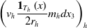$\left( v_{h}\dfrac{\boldsymbol{1}_{T_{h}}\left(x\right) }{2r_{h}}m_{h}dx_{3}\right) _{h}$ converges to some $\chi $ . Let $\varphi \in C_{0}\left( \mathbb{R}^{3}\right) $ , we have, using Fenchel’s inequality

\begin{equation*}\left.\begin{array}{l}\underset{h\rightarrow \infty }{\lim \inf }\dfrac{1}{2r_{h}}\int_{-r_{h}}^{r_{h}}\int\nolimits_{\Sigma }\left\vert v_{h}\right\vert^{2}dm_{h}dx_{3} \\ \geq \underset{h\rightarrow \infty }{\lim \inf }\left( \int_{\mathbb{R}^{3}}v_{h}\varphi \dfrac{\boldsymbol{1}_{T_{h}}\left( x\right) }{2r_{h}}dm_{h}dx_{3}-\dfrac{1}{2}\int_{\mathbb{R}^{3}}\varphi ^{2}\dfrac{\boldsymbol{1}_{T_{h}}\left( x\right) }{2r_{h}}dm_{h}dx_{3}\right) \\ \geq \left\langle \chi ,\varphi \right\rangle -\dfrac{1}{2\mathcal{H}^{d}\left( \Sigma \right) }\int_{\Sigma }\varphi ^{2}\left( s,0\right) d\mathcal{H}^{d}\left( s\right)\! \text{.}\end{array}\right.\end{equation*}

As the left hand side of this inequality is bounded, we deduce that

\begin{equation*}\sup \left\{ \left\langle \chi ,\varphi \right\rangle \text{; }\varphi \in C_{0}\left( \mathbb{R}^{3}\right) \text{, }\dfrac{1}{\mathcal{H}^{d}\left(\Sigma \right) }\int_{\Sigma }\varphi ^{2}\left( s,0\right) d\mathcal{H}^{d}\left( s\right) \leq 1\right\} <+\infty \text{,}\end{equation*}

from which we deduce, according to Riesz’ representation Theorem, that there exists v, such that $v\in L_{\mathcal{H}^{d}}^{2}\left( \Sigma \right) $ and $\chi =v\boldsymbol{1}_{\Sigma }\left( s\right) \dfrac{d\mathcal{H}^{d}\left( s\right) \otimes \delta _{0}\left( x_{3}\right) }{\mathcal{H}^{d}\left( \Sigma \right) }$ .

Proposition 10 Let $\left( u^{h}\right) _{h}$ ; $u^{h}\in H\left( \Omega _{h},\mathbb{R}^{3}\right) $ , be a sequence such that

\begin{equation*}\sup_{h}\int_{T_{h}}\sigma _{ij}^{\ast h}\left( u^{h}\right) e_{ij}\left(u^{h}\right) dsdx_{3}<+\infty \text{.}\end{equation*}

Then, under the assumption (2.20), there exists a subsequence, still denoted $\left( u^{h}\right) _{h}$ , such that

1. 1. $u_{\alpha }^{h}\dfrac{\boldsymbol{1}_{T_{h}}\left( x\right) }{2r_{h}}m_{h}dx_{3}\overset{\ast }{\underset{h\rightarrow \infty }{\rightharpoonup }}v_{\alpha }\boldsymbol{1}_{\Sigma }\left( s\right) \dfrac{d\mathcal{H}^{d}\left( s\right) \otimes \delta _{0}\left( x_{3}\right) }{\mathcal{H}^{d}\left( \Sigma \right) }$ , with $v_{\alpha }\left( s\right) \in L_{\mathcal{H}^{d}}^{2}\left( \Sigma \right) $ ; $\alpha =1,2$ ,

2. 2. $\varepsilon _{h}u_{3}^{h}\dfrac{\boldsymbol{1}_{T_{h}}\left( x\right)}{2r_{h}}m_{h}dx_{3}\overset{\ast }{\underset{h\rightarrow \infty }{\rightharpoonup }}0$ .

Proof. According to Lemma 5 $_{2,3}$ , we have, up to some subsequence,

\begin{equation*}\left.\begin{array}{l}u_{\alpha }^{h}\dfrac{\boldsymbol{1}_{T_{h}}\left( x\right) }{2r_{h}}m_{h}dx_{3}\overset{\ast }{\underset{h\rightarrow \infty }{\rightharpoonup }}v_{\alpha }\boldsymbol{1}_{\Sigma }\left( s\right) \dfrac{d\mathcal{H}^{d}\left( s\right) \otimes \delta _{0}\left( x_{3}\right) }{\mathcal{H}^{d}\left( \Sigma \right) }\text{; }\alpha =1,2\text{,} \\ \varepsilon _{h}u_{3}^{h}\dfrac{\boldsymbol{1}_{T_{h}}\left( x\right) }{2r_{h}}m_{h}dx_{3}\overset{\ast }{\underset{h\rightarrow \infty }{\rightharpoonup }}0\text{,}\end{array}\right.\end{equation*}

with $v_{\alpha }\in L_{\mathcal{H}^{d}}^{2}\left( \Sigma \right) $ ; $\alpha=1,2$ .

5 The main result

In this section, we state the main result of this work. According to Propositions 8 and 10, we introduce the following topology $\tau $ :

Definition 11 We say that a sequence $\left( u^{h}\right) _{h}$ ; $u^{h}\in H\left( \Omega _{h},\mathbb{R}^{3}\right) $ , $\tau $ -converges to $\left(u,v\right) $ ; $v=\left( v_{1},v_{2}\right) $ , if u is independent of $z\in$ $\left( -1,1\right) $ , $u_{\alpha }\left( x^{\prime }\right)=\int_{-1}^{1}U_{\alpha }\left( x^{\prime },z\right) dz$ ; $\alpha =1,2$ , and

\begin{equation*}\left\{\begin{array}{l}u_{\alpha }^{h}\overset{dr}{\rightharpoonup }U_{\alpha } \, L^{2}\left( \omega \times \left( -1,1\right) ,\mathbb{R}^{3}\right) \text{; }\alpha =1,2\text{,} \\ \varepsilon _{h}u_{3}^{h}\overset{dr}{\rightharpoonup }u_{3} \, L^{2}\left( \omega \times \left( -1,1\right) ,\mathbb{R}^{3}\right) \text{,}\\ u_{\alpha }^{h}\dfrac{\boldsymbol{1}_{T_{h}}\left( x\right) }{2r_{h}}m_{h}dx_{3}\overset{\ast }{\underset{h\rightarrow \infty }{\rightharpoonup }}v_{\alpha }\boldsymbol{1}_{\Sigma }\left( s\right) \dfrac{d\mathcal{H}^{d}\left( s\right) \otimes \delta _{0}\left( x_{3}\right) }{\mathcal{H}^{d}\left( \Sigma \right) }\text{ in }\mathcal{M}\left( \mathbb{R}^{3}\right) \text{; }\alpha =1,2\text{,} \\ \varepsilon _{h}u_{3}^{h}\dfrac{\boldsymbol{1}_{T_{h}}\left( x\right) }{2r_{h}}m_{h}dx_{3}\overset{\ast }{\underset{h\rightarrow \infty }{\rightharpoonup }}0\text{ in }\mathcal{M}\left( \mathbb{R}^{3}\right) \text{.}\end{array}\right.\end{equation*}

We state our main result of the $\Gamma $ -convergence in the topology $\tau $ of the sequence of functionals $F_{h}$ to the functional $F_{\infty }$ defined in (1.1) as follows:

Let us write the associated homogenised problem obtained at the limit as $h\longrightarrow \infty $ .

Corollary 13 Problem (2.28) admits a unique solution $u^{h}$ which, under the hypotheses of Theorem 12, $\tau $ -converges to $\left( u,v\right) $ $\in H\left( \omega ,\mathbb{R}^{3}\right) $ such that

\begin{equation*}\underset{h\rightarrow \infty }{\lim }F_{h}\left( u^{h}\right) =F_{\infty}\left( u,v\right)\end{equation*}

and $\left( u,v\right) $ is the solution of the problem

$$\left\{ {\matrix{ {\;\;\;\;\;\;\;{{ - }}{\eta _{\alpha \beta ,\beta }}\left( {{{\bar u}}} \right)} \hfill & = \hfill & {{{ }}{{\tilde f}_\alpha }{{; }}\alpha = 1,2{{,}}} \hfill & {{{in }} \, \omega {{,}}} \hfill \cr {\;\;\;\;\;\;{{{\partial ^{{2}}}{\varpi _{\alpha \beta }}\left( {{{{u}}_{{3}}}} \right)} \over {\partial {{{x}}_\alpha }\partial {{{x}}_\beta }}}} \hfill & = \hfill & {{{ }}{{\tilde f}_3}} \hfill & {{{in }} \, \omega {{,}}} \hfill \cr {\;{{ - }}{\mu ^ * }{\Delta _{\alpha ,\Sigma }}\left( {{v}} \right)} \hfill & = \hfill & {\mu \gamma {A_{\alpha \alpha }}\left( s \right)\left( {{u_\alpha } - {v_\alpha }} \right){{; }}\alpha = 1,2{{,}}} \hfill & {{{in }} \, \Sigma {{,}}} \hfill \cr {\;\;\;\;\;{{\left[ {{\eta _{\alpha \beta }}\left( {{{\bar u}}} \right){\nu _\beta }} \right]}_\Sigma }} \hfill & = \hfill & {{{\pi \mu \gamma } \over {{{\cal H}^d}\left( \Sigma \right){{\left( {\ln 2} \right)}^2}}}{A_{\alpha \alpha }}\left( s \right)\left( {{u_\alpha } - {v_\alpha }} \right){{\cal H}^d}{{ }}} \hfill & {{{on }} \, \Sigma {{,}}} \hfill \cr {{{ }}{{\left[ {{\varpi _{\alpha \beta }}\left( {{u_3}} \right){\nu _\beta }} \right]}_\Sigma }\;\;} \hfill & = \hfill & 0 \hfill & {{{on }} \, \Sigma {{,}}} \hfill \cr {} \hfill & {} \hfill & {} \hfill & {} \hfill \cr {{{\left[ {{{\partial {\varpi _{\alpha \beta }}\left( {{u_3}} \right)} \over {\partial {x_\alpha }}}{\nu _\beta }} \right]}_\Sigma }} \hfill & = \hfill & {{{\pi \mu \gamma } \over {{{\cal H}^d}\left( \Sigma \right)\left( {1 + \kappa } \right){{\left( {\ln 2} \right)}^2}}}{u_3}{{ }}} \hfill & {{{on }} \, \Sigma {{,}}} \hfill \cr {\;\;\;\;\;\;\;\;\;\;\;\;\;\;\;\;\;\;\;\;\;\;\;\;{u}} \hfill & = \hfill & 0 \hfill & {{{on}}\;\partial \omega {{,}}} \hfill \cr {\;\;\;\;\;\;\;\;\;\;\;\;\;\;\;\;\;\;\;\;\;\;\;{v}} \hfill & = \hfill & 0 \hfill & {{{on }} \, \Sigma \cap \partial \omega {{,}}} \hfill \cr } } \right.$$

where $\ \nu $ is the unit normal on $\Sigma $ and $\widetilde{f_{i}}\left(x_{1},x_{2}\right) =\int_{-1}^{1}f_{i}\left( x_{1},x_{2},x_{3}\right) dx_{3}$ ; $i=1,2,3$ .

Proof. One can easily check that problem (2.28) has a unique solution $u^{h}\in H_{0}^{1}\left( \Omega ,\mathbb{R}^{3}\right) \cap H^{1}\left(T_{h},\mathbb{R}^{3}\right) $ . Now, observing that

\begin{equation*}F_{h}\left( u^{h}\right) -2\int_{\Omega _{h}}f.u^{h}dx\leq F_{h}\left(0\right) =0\text{,}\end{equation*}

we deduce, using the fact that $\underset{h\rightarrow \infty }{\lim }c_{h}=+\infty $ , and the inequalities (4.1) and (4.2) of the proof of Lemma 4, that

\begin{equation*}\left.\begin{array}{l}\underset{\alpha ,\beta =1,2}{\sum }\dfrac{1}{\varepsilon _{h}}\int_{\Omega_{h}}\left( u_{\alpha }^{h}\right) ^{2}dx+\dfrac{1}{\varepsilon _{h}}\int_{\Omega _{h}}\left( \varepsilon _{h}u_{3}^{h}\right) ^{2}dx \\ \leq F_{h}\left( u_{h}\right) \leq 2\int_{\Omega _{h}}f.u_{h}dx \\ \leq 2\left( \dfrac{1}{\varepsilon _{h}}\int_{\Omega _{h}}\left\vert f\right\vert ^{2}dx\right) ^{1/2}\left( \dfrac{1}{\varepsilon _{h}}\int_{\Omega _{h}}^{2}\left\vert \varepsilon _{h}u^{h}\right\vert^{2}dx\right) ^{1/2} \\ \leq C\left( \dfrac{1}{\varepsilon _{h}}\int_{\Omega _{h}}^{2}\left\vert\varepsilon _{h}u^{h}\right\vert ^{2}dx\right) ^{1/2}\text{,}\end{array}\right.\end{equation*}

from which we deduce, in particular, that $\sup_{h}F_{h}\left( u^{h}\right)<+\infty $ . Then, in view of Propositions 8, 10, and Theorem 12, we deduce, according to [Reference Dal Maso11, Theorem 7.8]), that the sequence $\left( u^{h}\right) _{h}$ $\tau $ -converges to the solution $\left( u,v\right) $ $\in H\left( \omega ,\mathbb{R}^{3}\right) $ of the problem

(5.1) \begin{equation}\underset{\left( \xi ,\zeta \right) \in H\left( \omega ,\mathbb{R}^{3}\right) }{\min }\left\{\begin{array}{l}\int_{\omega }\eta _{\alpha \beta }\left( \xi \right) e_{\alpha \beta}\left( \xi \right) dx^{\prime }+\mu ^{\ast }\int_{\Sigma }d\mathcal{L}_{\Sigma }\left( \zeta \right) \\ +\dfrac{\pi \mu \gamma }{\mathcal{H}^{d}\left( \Sigma \right) \left( \ln2\right) ^{2}}\int\nolimits_{\Sigma }A_{\alpha \alpha }\left( s\right)\left( \xi _{\alpha }-\zeta _{\alpha }\right) ^{2}d\mathcal{H}^{d}\left(s\right) \\ +\dfrac{\pi \mu \gamma }{\mathcal{H}^{d}\left( \Sigma \right) \left( \ln2\right) ^{2}}\int\nolimits_{\Sigma }A_{33}\left( s\right) \xi _{3}^{2}d\mathcal{H}^{d}\left( s\right) \\ +\int_{\omega }\varpi _{\alpha \beta }\left( \xi _{3}\right) \dfrac{\partial^{2}\xi _{3}}{\partial x_{\alpha }\partial x_{\beta }}dx^{\prime } \\ -2\int_{\omega }\widetilde{f_{i}}\xi _{i}dx^{\prime }\text{,}\end{array}\right\} \end{equation}

and

\begin{equation*}\underset{h\rightarrow \infty }{\lim }F_{h}\left( u^{h}\right) =F_{\infty}\left( u,v\right) \text{.}\end{equation*}

The trace of an element of $H^{1}\left( \omega ,\mathbb{R}^{2}\right) $ on $\omega \cap \Sigma $ exists for $\mathcal{H}^{d}$ -almost-every $x\in \omega\cap \Sigma $ and belongs to the Besov space $B_{d/2}^{2}\left( \Sigma ,\mathbb{R}^{2}\right) $ defined by

(5.2) \begin{equation}\text{ }B_{d/2}^{2}\left( \Sigma ,\mathbb{R}^{2}\right) =\left\{\begin{array}{l}v\,{:}\,\Sigma \longrightarrow \mathbb{R}^{2}\text{; }\int_{\Sigma }\left\vert v\left( x\right) \right\vert ^{2}d\mathcal{H}^{d}\left( x\right) \\ +\underset{\left\vert x-y\right\vert <1}{\int_{\Sigma }\int_{\Sigma }}\dfrac{\left\vert v\left( x\right) -v\left( y\right) \right\vert ^{2}}{\left\vert x-y\right\vert ^{2d}}d\mathcal{H}^{d}\left( x\right) d\mathcal{H}^{d}\left(y\right) <+\infty\end{array}\right\} \text{,} \end{equation}

see [Reference Jonsson and Wallin24, Theorem 6]. More details on Besov spaces $B_{\alpha}^{p,q}\left( K\right) $ , $\alpha >0$ , $1\leq p,q\leq \infty $ , defined for a large class of closed subsets K of $\mathbb{R}^{N}$ including fractal subsets, can be found in [Reference Jonsson and Wallin22, Chapters 5 and 6]. In our case $K=\Sigma $ , $\alpha =d/2$ , and $p=q=2$ . The trace Theorem [Reference Jonsson and Wallin24, Theorem 6] can be applied to a more geometrically complex domain which, supplied with a positive Borel measure, is a d-set preserving Markov’s inequality [Reference Jonsson and Wallin24, pp. 193--195]. Typical examples of d-sets are self-similar fractals (see for instance [Reference Jonsson and Wallin24, pp. 194]). According to [Reference Jonsson and Wallin22, Theorem 3, p. 39], if $K\subset R^{N}$ is a d-set with $d>N-1$ , then K preserves Markov’s inequality. In particular, the Sierpinski carpet $\Sigma $ is a d-set preserving Markov’s inequality where d is the fractal dimension of $\Sigma $ given in (1.4). Then, using Lemma 3, we obtain from (5.1) that $v\in\mathcal{D}_{\Delta _{\Sigma }}$ and for every $\left( \xi ,\zeta \right)\in H\left( \omega ,\mathbb{R}^{3}\right) $ ,

(5.3) \begin{equation}\begin{array}{l}\int_{\omega }\left( -\eta _{\alpha \beta ,\beta }\left( \overline{u}\right)-\widetilde{f_{\alpha }}\right) \xi _{\alpha }dx^{\prime }-\dfrac{\mu ^{\ast}}{\mathcal{H}^{d}\left( \Sigma \right) }\int_{\Sigma }\left( \Delta_{\alpha ,\Sigma }v\right) \zeta _{\alpha }d\mathcal{H}^{d} \\ +\dfrac{\pi \mu \gamma }{\mathcal{H}^{d}\left( \Sigma \right) }\underset{\alpha =1,2}{\sum }\int\nolimits_{\Sigma }A_{\alpha \alpha }\left( s\right)\left( u_{\alpha }-v_{\alpha }\right) \left( \xi _{\alpha }-\zeta _{\alpha}\right) d\mathcal{H}^{d}\left( s\right) \\ +\dfrac{\pi \mu \gamma }{\mathcal{H}^{d}\left( \Sigma \right) }\int\nolimits_{\Sigma }A_{33}\left( s\right) u_{3}\xi _{3}d\mathcal{H}^{d}\left( s\right) \\ +\int_{\omega }\left( \dfrac{\partial ^{2}\varpi _{\alpha \beta }\left(u_{3}\right) }{\partial x_{\alpha }\partial x_{\beta }}-\widetilde{f_{3}}\right) \xi _{3}dx^{\prime } \\ +\left\langle \left[ \varpi _{\alpha \beta }\left( u_{3}\right) \nu _{\beta }\right] _{\Sigma },\dfrac{\partial \xi _{3}}{\partial x_{\alpha }}\right\rangle _{B_{-d/2}^{2}\left( \Sigma ,\mathbb{R}^{3}\right),B_{d/2}^{2}\left( \Sigma ,\mathbb{R}^{3}\right) } \\ -\left\langle \left[ \dfrac{\partial \varpi _{\alpha \beta }\left(u_{3}\right) }{\partial x_{\alpha }}\nu _{\beta }\right] _{\Sigma },\xi_{3}\right\rangle _{B_{-d/2}^{2}\left( \Sigma ,\mathbb{R}^{3}\right),B_{d/2}^{2}\left( \Sigma ,\mathbb{R}^{3}\right) } \\ +\left\langle \left[ \eta _{\alpha \beta }\left( \overline{u}\right) \nu_{\beta }\right] _{\Sigma },\xi _{\alpha }\right\rangle _{B_{-d/2}^{2}\left(\Sigma ,\mathbb{R}^{3}\right) ,B_{d/2}^{2}\left( \Sigma ,\mathbb{R}^{3}\right) }=0\text{,}\end{array}. \end{equation}

where $B_{-d/2}^{2}\left( \Sigma ,\mathbb{R}^{3}\right) $ is the dual space of $B_{d/2}^{2}\left( \Sigma ,\mathbb{R}^{3}\right) $ (see [Reference Jonsson and Wallin23, p. 291]).

6 Proof of the main result

This section is devoted to the proof of the main results. We first study a local problem which is related to boundary layers due to the local interactions between the constituent materials. The solution of this local problem is crucial in constructing appropriate test functions in order to pass to the limit in the original problem.

6.1 Local problems

We consider here some local problems associated with boundary layers in the vicinity of the ribbons. We denote $w^{m}$ ; $m=1,2$ , the solution of the following boundary value problem:

(6.1) \begin{equation}\left\{\begin{array}{rcll}\operatorname{div} \sigma \left( w^{m}\right) \left( y\right) & = & 0 & \forall y\in\mathbb{R}^{2+} \\ w^{m}\left( y_{1},0\right) & = & \left( \delta _{1m},\delta _{2m}\right) &\forall y_{1}\in \left] -1,1\right[ \text{,} \\ \sigma _{i2}\left( w^{m}\right) \left( y\right) & = & 0 & \forall y\in\left( \mathbb{R}\setminus \left] -1,1\right[ \right) \times \left\{0\right\} \text{,} \\ w_{m}^{m}\left( y\right) & = & -\dfrac{\ln \left\vert y\right\vert }{\ln 2}& \text{when }\left\vert y\right\vert \rightarrow \infty \text{, }y_{2}>0\text{,} \\ \left\vert w_{p}^{m}\right\vert \left( y\right) & \leq & C & \text{when }\left\{\begin{array}{l}p=2\text{ if }m=1\text{,} \\ p=1\text{ if }m=2\text{,}\end{array}\right.\end{array}\right. \end{equation}

where $\sigma _{ij}\left( w^{m}\right) =\lambda e_{kk}\left( w^{m}\right)\delta _{ij}+2\mu e_{ij}\left( w^{m}\right) $ ; $i,j=1,2$ and

\begin{equation*}\mathbb{R}^{2+}=\left\{ y=\left( y_{1},y_{2}\right) \in \mathbb{R}^{2}\text{; }y_{2}>0\right\} .\end{equation*}

The displacement $w^{m}$ ; $m=1,2$ , which belongs to the space $H_{loc}^{1}\left( \mathbb{R}^{2+},\mathbb{R}^{2}\right) $ , is given (see for instance [Reference El Jarroudi12, Reference El Jarroudi and Er-Riani14, Reference Lobo and Perez29]) by

(6.2) \begin{equation}\left\{\begin{array}{lll}w_{1}^{1}\left( y\right) & = & -\dfrac{1+\kappa }{4\pi \mu }\int\nolimits_{-1}^{1}\theta \left( t\right) \ln \left( \sqrt{\left(y_{1}-t\right) ^{2}+y_{2}^{2}}\right) dt\text{} \\& & +\dfrac{1}{4\pi \mu }\int\nolimits_{-1}^{1}\theta \left( t\right)\dfrac{2y_{2}^{2}}{\left( y_{1}-t\right) ^{2}+y_{2}^{2}}dt\text{,} \\w_{2}^{1}\left( y\right) & = & -\dfrac{\left( 1-\kappa \right) }{4\pi \mu }\int\nolimits_{-1}^{1}\theta \left( t\right) \arctan \left( \dfrac{y_{2}}{y_{1}-t}\right) dt \\& & +\dfrac{1}{4\pi \mu }\int\nolimits_{-1}^{1}\theta \left( t\right)\dfrac{2y_{2}\left( y_{1}-t\right) }{\left( y_{1}-t\right) ^{2}+y_{2}^{2}}dt\end{array}\right. \end{equation}

and

(6.3) \begin{equation}\left\{\begin{array}{lll}w_{1}^{2}\left( y\right) & = & \dfrac{\left( 1-\kappa \right) }{4\pi \mu }\int\nolimits_{-1}^{1}\theta \left( t\right) \arctan \left( \dfrac{y_{2}}{y_{1}-t}\right) dt \\& & +\dfrac{1}{4\pi \mu }\int\nolimits_{-1}^{1}\theta \left( t\right)\dfrac{2y_{2}\left( y_{1}-t\right) }{\left( y_{1}-t\right) ^{2}+y_{2}^{2}}dt\text{,} \\w_{2}^{2}\left( y\right) & = & -\dfrac{\left( 1+\kappa \right) }{4\pi \mu }\int\nolimits_{-1}^{1}\theta \left( t\right) \ln \left( \sqrt{\left(y_{1}-t\right) ^{2}+y_{2}^{2}}\right) dt \\& & -\dfrac{1}{4\pi \mu }\int\nolimits_{-1}^{1}\theta \left( t\right)\dfrac{2y_{2}^{2}}{\left( y_{1}-t\right) ^{2}+y_{2}^{2}}\text{,}\end{array}\right. \end{equation}

where

(6.4) \begin{equation}\theta \left( t\right) =\left\{\begin{array}{l@{\quad}l}\dfrac{4\mu }{\left( 1+\kappa \right) \ln 2}\dfrac{1}{\sqrt{1-t^{2}}} &\text{if }t\in \left] -1,1\right[ \text{,} \\ 0 & \text{otherwise.}\end{array}\right. \end{equation}

One can check that $w^{m}\left( y\right) $ ; $m=1,2$ , is also the solution of problem (6.1) posed in the half-plane $\mathbb{R}^{2-}$ :

\begin{equation*}\mathbb{R}^{2-}=\left\{ y=\left( y_{1},y_{2}\right) \in \mathbb{R}^{2}\text{; }y_{2}<0\right\} \text{.}\end{equation*}

We introduce the following scalar problem:

(6.5) \begin{equation}\left\{\begin{array}{rcll}\Delta w\left( y\right) & = & 0 & \forall y\in \mathbb{R}^{2+}\text{,} \\w\left( y_{1},0\right) & = & 1 & \forall y_{1}\in \left] -1,1\right[ \text{,}\\\dfrac{\partial w}{\partial y_{2}}\left( y_{1},0\right) & = & 0 & \forall y_{1}\in \mathbb{R}\setminus \left] -1,1\right[ \text{,} \\w\left( y\right) & = & -\dfrac{\ln \left\vert y\right\vert }{\ln 2} & \text{as }\left\vert y\right\vert \rightarrow \infty \text{, }y_{2}>0\text{.}\end{array}\right. \end{equation}

The solution of (6.5) is given by

(6.6) \begin{equation}w\left( y\right) =-\dfrac{1}{\pi \ln 2}\int\nolimits_{-1}^{1}\frac{\ln\left( \sqrt{\left( y_{1}-t\right) ^{2}+y_{2}^{2}}\right) }{\sqrt{1-t^{2}}}dt\text{.} \end{equation}

Observe that $w\left( y\right) $ is also the solution of problem (6.5) posed in the half-plane $\mathbb{R}^{2-}$ . We now state the following preliminary result in this subsection:

Proposition 14 ([Reference El Jarroudi12, Proposition 7]). One has

1. 1. $\underset{R\rightarrow +\infty }{\lim }\dfrac{1}{\ln R}\int\nolimits_{B\left( 0,R\right) \cap \mathbb{R}^{2\pm }}\sigma _{ij}\left(w^{m}\right) e_{ij}\left( w^{l}\right) dy=\delta _{ml}\dfrac{2\mu \pi }{\left( 1+\kappa \right) \left( \ln 2\right) ^{2}}$ ,

2. 2. $\underset{R\rightarrow +\infty }{\lim }\dfrac{1}{\ln R}\int\nolimits_{B\left( 0,R\right) \cap \mathbb{R}^{2\pm }}\left\vert \nabla w\right\vert ^{2}dy=\dfrac{\pi }{\left( \ln 2\right) ^{2}}$ , where $D\left(0,R\right) $ is a disk of radius R centred at the origin.

We define the rotation matrix $\mathcal{R}\left( x_{h}^{k}\right) $ ; $x_{h}^{k}=\left( x_{1h}^{k},x_{2h}^{k}\right) $ being the centre of $S_{h}^{k}$ ; $k\in I_{h}$ , by

(6.7) \begin{equation}\mathcal{R}\left( x_{h}^{k}\right) =\left\{\begin{array}{ll}Id_{\mathbb{R}^{3}} & \text{if }n^{k}=\pm e_{2}\text{,} \\& \\\left(\begin{array}{c@{\quad}c@{\quad}c}0 & 1 & 0 \\[3pt]1 & 0 & 0 \\[3pt]0 & 0 & 1\end{array}\right) & \text{if }n^{k}=\pm e_{1}\text{,}\end{array}\right. \end{equation}

where $Id_{\mathbb{R}^{3}}$ is the $3\times 3$ identity matrix and $n^{k}$ is the unit normal to the line segment $S_{h}^{k}$ , in the plane xOy. Let $\varphi _{h}^{k}$ ; $k\in I_{h}$ , be the truncation function defined on $\mathbb{R}^{2}$ by

(6.8) \begin{equation}\varphi _{h}^{k}\left( x\right) =\left\{\begin{array}{l@{\quad}l}\dfrac{4\left( 3^{-2h}-4R_{k,h}^{2}\left( x\right) \right) }{3^{-2h+1}} &\text{if }3^{-h}/4\leq R_{h}^{k}\left( x\right) \leq 3^{-h}/2\text{,} \\ 1 & \text{if }R_{h}^{k}\left( x\right) \leq 3^{-h}/4\text{,} \\ 0 & \text{if }R_{h}^{k}\left( x\right) \geq 3^{-h}/2\text{,}\end{array}\right. \end{equation}

where $R_{h}^{k}\left( x\right) =\sqrt{\left( \left( x-x_{h}^{k}\right).n^{k}\right) ^{2}+x_{3}^{2}}$ . We define, for $k\in I_{h}$ ,

(6.9) \begin{equation}D_{h}^{k}\left( s_{h}\right) =\left\{ \left( \left( x-x_{h}^{k}\right).n^{k},x_{3}\right) \in \mathbb{R}^{2}\text{; }R_{h}^{k}\left( x\right)<3^{-h}/2\text{, }\forall x\in \mathbb{R}^{3}\right\} \end{equation}

and the cylinder

(6.10) \begin{equation}Z_{h}^{k}=\mathcal{R}\left( x_{h}^{k}\right) S_{h}^{k}\times D_{h}^{k}\left(s_{h}\right) \text{; }k\in I_{h}\text{.} \end{equation}

We then set

(6.11) \begin{equation}Z_{h}=\underset{k\in I_{h}}{\bigcup }Z_{h}^{k}\text{.} \end{equation}

Let $k\in I_{h}$ . We set $\Phi _{h}^{k}\left( x\right) =\varphi_{h}^{k}\left( x\right) \mathcal{R}\left( x_{h}^{k}\right) $ and define the function $w_{h}^{mk}\left( x\right) $ ; $m=1,2,3$ , by

(6.12) \begin{equation}w_{h}^{1k}\left( x\right) =\Phi _{h}^{k}\left( x\right) \left( e_{1}-\frac{1}{\ln r_{h}}\left(\begin{array}{c}1-w\left( \dfrac{x_{3}}{r_{h}},\dfrac{\left( x-x_{h}^{k}\right) .n^{k}}{r_{h}}\right) \\0 \\0\end{array}\right) \right) \text{,} \end{equation}

(6.13) \begin{equation}w_{h}^{2k}\left( x\right) =\Phi _{h}^{k}\left( x\right) \left( e_{2}-\frac{1}{\ln r_{h}}\left(\begin{array}{c}0 \\1-w_{1}^{1}\left( \dfrac{x_{3}}{r_{h}},\dfrac{\left( x-x_{h}^{k}\right).n^{k}}{r_{h}}\right) \\w_{2}^{1}\left( \dfrac{x_{3}}{r_{h}},\dfrac{\left( x-x_{h}^{k}\right) .n^{k}}{r_{h}}\right)\end{array}\right) \right) \end{equation}

and

(6.14) \begin{equation}w_{h}^{3k}\left( x\right) =\Phi _{h}^{k}\left( x\right) \left( e_{3}-\frac{\varepsilon _{h}}{\ln r_{h}}\left(\begin{array}{c}0 \\w_{1}^{2}\left( \dfrac{x_{3}}{r_{h}},\dfrac{\left( x-x_{h}^{k}\right) .\nu^{k}}{r_{h}}\right) \\ w_{2}^{2}\left( \dfrac{x_{3}}{r_{h}},\dfrac{\left( x-x_{h}^{k}\right) .\nu^{k}}{r_{h}}\right)\end{array}\right) \right) \text{.} \end{equation}

where $e_{i}=\left( \delta _{1i},\delta _{2i},\delta _{3i}\right) $ . We define now the local perturbations $w_{h}^{m}$ ; $m=1,2,3$ , through

(6.15) \begin{equation}w_{h}^{m}\left( x\right) =w_{h}^{mk}\left( x\right) \text{, }\forall k\in I_{h}\text{, }\forall x\in \omega \times \left( \mathbb{-}1,1\right) \text{.}\end{equation}

Lemma 15 If $\gamma \in \left( 0,+\infty \right) $ then, under the assumption (2.25), for every $\Psi \in C^{1}\left( \overline{\omega }\times \left[ \mathbb{-}1,1\right] ,\mathbb{R}^{3}\right) $ and $\Psi^{h}=\left( \Psi _{1},\Psi _{2},\Psi _{3}/\varepsilon _{h}\right) $ , we have

\begin{equation*}\underset{h\rightarrow \infty }{\lim }\left( \int\nolimits_{Z_{h}}\sigma_{ij}^{h}\left( w_{h}^{l}\Psi _{m}^{h}\right) e_{ij}\left( w_{h}^{l^{\prime}}\Psi _{l}^{h}\right) dx\right) =\dfrac{\pi \mu \gamma }{\mathcal{H}^{d}\left( \Sigma \right) \left( \ln 2\right) ^{2}}\int\nolimits_{\Sigma}A\left( s\right) \Psi \left( s\right) .\Psi \left( s\right) d\mathcal{H}^{d}\left( s\right) \text{,}\end{equation*}

where $A\left( s\right) $ is the matrix defined in (1.6).

Proof. Let us introduce the local variables $y=\left( y_{1},y_{2}\right) $ with

(6.16) \begin{equation}\left\{\begin{array}{l}y_{1}=x_{3}/r_{h}\text{,} \\ y_{2}=\left( x-x_{h}^{k}\right) .n^{k}/r_{h}\text{.}\end{array}\right. \end{equation}

Then, using the smoothness of $\Psi $ , the assumption (2.25), and Proposition 14, we obtain that

(6.17) \begin{equation}\left.\begin{array}{l}\underset{h\rightarrow \infty }{\lim }\int\nolimits_{Z_{h}}\sigma_{ij}^{h}\left( w_{h}^{l}\Psi _{m}^{h}\right) e_{ij}\left( w_{h}^{l^{\prime}}\Psi _{l}^{h}\right) dx \\ =\underset{h\rightarrow \infty }{\lim }\underset{k\in I_{h}}{\sum }\int\nolimits_{Z_{h}^{k}}\sigma _{ij}^{h}\left( w_{h}^{lk}\right)e_{ij}\left( w_{h}^{l^{\prime }k}\right) \Psi _{m}^{h}\Psi _{l}^{h}dx \\ =\underset{h\rightarrow \infty }{\lim }\dfrac{b}{\dfrac{3^{h}}{8^{h}}\varepsilon _{h}\ln ^{2}r_{h}}\int\nolimits_{D\left( 0,\frac{3^{-h}}{2r_{h}}\right) \backslash D\left( 0,1\right) }\sigma _{ij}\left( w^{l}\right)e_{ij}\left( w^{l^{\prime }}\right) dy \\ \times \left( \underset{k=1}{\overset{N_{h}^{v}}{\sum }}\dfrac{a}{bN_{h}^{v}}\left( \mathcal{R}\left( x_{h}^{k}\right) \Psi \right) _{m}\left( \mathcal{R}\left( x_{h}^{k}\right) \Psi \right) _{l}\left( x_{1h}^{k},x_{2h}^{k}\right)\right) \\ =\dfrac{\pi \mu \gamma }{\mathcal{H}^{d}\left( \Sigma \right) \left( \ln2\right) ^{2}}\int\nolimits_{\Sigma }\left( D_{iag}\mathcal{R}\left(s\right) \Psi \left( s\right) \right) _{m}\left( \mathcal{R}\left( s\right)\Psi \left( s\right) \right) _{l}d\mathcal{H}^{d}\left( s\right) \\ =\dfrac{\pi \mu \gamma }{\mathcal{H}^{d}\left( \Sigma \right) \left( \ln2\right) ^{2}}\int\nolimits_{\Sigma }\mathcal{R}^{t}\left( s\right) D_{iag}\mathcal{R}\left( s\right) \Psi \left( s\right) .\Psi \left( s\right) d\mathcal{H}^{d}\left( s\right) \text{,}\end{array}\right. \end{equation}

where $D\left( 0,\dfrac{3^{-h}}{2r_{h}}\right) $ is the disk of radius $\dfrac{3^{-h}}{2r_{h}}$ centred at the origin, D(0,1) is the disk of radius 1 centred at the origin, $D_{iag}=$ Diag $\left( 1,\dfrac{2}{\left(1+\kappa \right) },\dfrac{2}{\left( 1+\kappa \right) }\right) $ , and $\mathcal{R}\left( s\right) $ is the rotation matrix defined by $\mathcal{R}\left( s\right) $ $=Id_{\mathbb{R}^{3}}$ on the face of $\Sigma $ which is perpendicular to the vector $e_{2}$ and by $\mathcal{R}\left( s\right)=\left(\begin{array}{c@{\quad}c@{\quad}c}0 & 1 & 0 \\1 & 0 & 0 \\0 & 0 & 1\end{array}\right) $ on the face of $\Sigma $ which is perpendicular to the vector $e_{1}$ . Observing that in (6.17)

\begin{equation*}\mathcal{R}^{t}\left( s\right) D_{iag}\mathcal{R}\left( s\right) =\mathcal{R}\left( s\right) D_{iag}\mathcal{R}\left( s\right) =A\left( s\right) \text{,}\end{equation*}

we obtain the desired result.

6.2 Proof of Theorem 12

The proof of Theorem 12 is given in two steps.

6.2.1 Step 1: Lim-sup inequality

Here we prove the lim-sup property of the $\Gamma $ -convergence stated in Theorem 12. We first construct a test function on each line segment $S_{h}^{k}$ ; $k\in I_{h}$ , with extremities $p_{h}^{k}=\left(p_{h1}^{k},p_{h2}^{k}\right) $ , $q_{h}^{k}=\left(q_{h1}^{k},q_{h2}^{k}\right), $ and centre $x_{h}^{k}=\left(x_{h1}^{k},x_{h2}^{k}\right) $ . Let $\left( v_{1},v_{2},v_{3}\right) \in C_{c}^{2}\left( \omega ,\mathbb{R}^{3}\right) $ . We consider the sequence $\left( v^{h,k}\right) _{h}$ of test functions defined, for every $x=\left(x_{1},x_{2}\right) \in S_{h}^{k}$ , by

(6.18) \begin{equation}\begin{array}{lll}v_{1}^{h,k}\left( x^{\prime }\right) & = & v_{1}\left(x_{1h}^{k},x_{2h}^{k}\right) +3^{h}\vartheta _{h}^{1,k}\left( x^{\prime}\right) \left\vert v_{1}\left( p_{h}^{k}\right) -v_{1}\left(q_{h}^{k}\right) \right\vert \text{,} \\ v_{2}^{h,k}\left( x^{\prime }\right) & = & v_{2}\left(x_{1h}^{k},x_{2h}^{k}\right) +3^{h}\vartheta _{h}^{2,k}\left( x^{\prime}\right) \left\vert v_{2}\left( p_{h}^{k}\right) -v_{2}\left(q_{h}^{k}\right) \right\vert \text{,} \\ v_{3}^{h,k}\left( x^{\prime }\right) & = & v_{3}\left(x_{1h}^{k},x_{2h}^{k}\right) \text{,}\end{array}\end{equation}

where $\vartheta _{h}^{i,k}\left( x^{\prime }\right) $ ; $i=1,2,3$ , is defined by

(6.19) \begin{equation}\left\{\begin{array}{lll}\vartheta _{h}^{1,k}\left( x^{\prime }\right) & = & \sqrt{\dfrac{\mu_{h}^{\ast }}{2}}\dfrac{\left( x_{1}-p_{h,1}^{k}\right) +\left(x_{1}-q_{h,1}^{k}\right) }{\sqrt{\lambda _{h}^{\ast }+2\mu _{h}^{\ast }}} \\ & & -\dfrac{\left( x_{2}-p_{h,2}^{k}\right) +\left(x_{2}-q_{h,2}^{k}\right) }{\sqrt{2}}\text{,} \\ \vartheta _{h}^{2,k}\left( x^{\prime }\right) & = & \sqrt{\dfrac{\mu_{h}^{\ast }}{2}}\dfrac{\left( x_{2}-p_{h,2}^{k}\right) +\left(x_{2}-q_{h,2}^{k}\right) }{2\sqrt{\lambda _{h}^{\ast }+2\mu _{h}^{\ast }}}\\ & & -\dfrac{\left( x_{1}-p_{h,1}^{k}\right) +\left(x_{1}-q_{h,1}^{k}\right) }{\sqrt{2}}\text{.}\end{array}\right. \end{equation}

Let us now introduce the intervals $J_{h}^{p_{h}^{k}}$ and $J_{h}^{q_{h}^{k}} $ which are centred at the points $p_{h}^{k}$ and $q_{h,}^{k}$ respectively, such that

(6.20) \begin{equation}S_{h}^{k}\cap J_{h}^{p_{h}^{k}}=\left[ p_{h}^{k},p_{h}^{k}+\textbf{l}_{h}\right) \text{, }S_{h}^{k}\cap J_{h}^{q_{h}^{k}}=\left( q_{h}^{k}-\textbf{l}_{h},q_{h}^{k}\right] \text{,} \end{equation}

where $\textbf{l}_{h}=\left(\begin{array}{c}l_{h} \\l_{h}\end{array}\right) $ so that $\underset{h\rightarrow \infty }{\lim }3^{h}l_{h}=0$ . Let $\psi _{h}^{k}$ be a $C_{c}^{\infty }\left( S_{h}^{k}\cup J_{h}^{p_{h}^{k}}\cup J_{h}^{q_{h}^{k}}\right) $ -mollifier such that

(6.21) \begin{equation}\psi _{h}^{k}=\left\{\begin{array}{ll}1 & \text{on} \, S_{h}^{k}\backslash J_{h}^{p_{h}^{k}}\cup J_{h}^{q_{h}^{k}}\text{,} \\ 0 & \text{on} \, J_{h}^{p_{h}^{k}}\cup J_{h}^{q_{h}^{k}}\backslash \left(\left( p_{h}^{k},p_{h}^{k}+\textbf{l}_{h}\right) \cup \left( q_{h}^{k}-\textbf{l}_{h},q_{h}^{k}\right) \right) \text{.}\end{array}\right. \end{equation}

We define the test function $v_{0}^{h}$ on $T_{h}$ by

(6.22) \begin{equation}v^{h}=\psi _{h}^{k}v^{h,k}\text{ on }T_{h}^{k}\text{, }\forall k\in I_{h}\text{.} \end{equation}

We have the following result:

Lemma 16 Under the assumption (2.20) we have

1. 1. $v_{\alpha }^{h}\dfrac{\boldsymbol{1}_{T_{h}}\left( x\right) }{2r_{h}}m_{h}dx_{3}\overset{\ast }{\underset{h\rightarrow \infty }{\rightharpoonup }}v_{\alpha }\boldsymbol{1}_{\Sigma }\left( s\right) \dfrac{d\mathcal{H}^{d}\left( s\right) \otimes \delta _{0}\left( x_{3}\right) }{\mathcal{H}^{d}\left( \Sigma \right) }$ in $\mathcal{M}\left( \mathbb{R}^{3}\right) $ ; $\alpha =1,2$ ,

2. 2. $\varepsilon _{h}v_{3}^{h}\dfrac{\boldsymbol{1}_{T_{h}}\left( x\right)}{2r_{h}}m_{h}dx_{3}\overset{\ast }{\underset{h\rightarrow \infty }{\rightharpoonup }}0$ in $\mathcal{M}\left( \mathbb{R}^{3}\right) $ ,

3. 3. $\underset{h\rightarrow \infty }{\lim }\int_{T_{h}}\sigma _{ij}^{\ast h}\left( v^{h}\right) e_{ij}\left( v^{h}\right) dx\mathcal{=}\mu ^{\ast }\underset{h\rightarrow \infty }{\lim }\rho ^{h}\underset{\left[ p,q\right]\in S_{h}^{\alpha }}{\underset{p,q\in \mathcal{V}_{h},}{\underset{\alpha =1,2}{\sum }}}\left( v_{\alpha }\left( p\right) -v_{\alpha }\left( q\right)\right) ^{2}$ .

Proof. 1. Let $\varphi \in C_{0}\left( \mathbb{R}^{3}\right) $ . Then,

\begin{align*}\underset{h\rightarrow \infty }{\lim }\int_{\mathbb{R}^{3}}\varphi v_{\alpha}^{h}\dfrac{\boldsymbol{1}_{T_{h}}\left( x\right) }{2r_{h}}m_{h}dx_{3}&=\underset{h\rightarrow \infty }{\lim }\underset{k\in I_{h}}{\sum }\dfrac{1}{N_{h}^{e}}v\left( x_{h1}^{k},x_{h2}^{k}\right) \varphi \left(x_{h1}^{k},x_{h2}^{k},0\right) \\[3pt]&\quad +\underset{h\rightarrow \infty }{\lim }\underset{k\in I_{h}}{\underset{\alpha =1,2}{\sum }}\dfrac{\vartheta _{h}^{\alpha ,k}\left(x_{h1}^{k},x_{h2}^{k}\right) }{N_{h}^{e}}\varphi \left(x_{h1}^{k},x_{h2}^{k},0\right) \text{.}\end{align*}

According to [Reference Falconer17, Theorem 6.1], we have

\begin{equation*}\left.\begin{array}{r}\underset{h\rightarrow \infty }{\lim }\underset{k\in I_{h}}{\sum }\dfrac{1}{N_{h}^{e}}v\left( x_{h1}^{k},x_{h2}^{k}\right) \varphi \left(x_{h1}^{k},x_{h2}^{k},0\right) =\underset{h\rightarrow \infty }{\lim }\underset{p\in \mathcal{V}_{h}}{\sum }\dfrac{v\left( p\right) \varphi \left(p,0\right) }{N_{h}^{v}} \\ =\dfrac{1}{\mathcal{H}^{d}\left( \Sigma \right) }\int_{\Sigma }v\left(s\right) \varphi \left( s,0\right) d\mathcal{H}^{d}\left( s\right) \text{.}\end{array}\right.\end{equation*}

Observing that, for every $h\in \mathbb{N}^{\ast }$ and every $k\in I_{h}$ ,

\begin{equation*}\left\vert v_{\alpha }\left( p_{h}^{k}\right) -v_{\alpha }\left(q_{h}^{k}\right) \right\vert \leq C\left\vert p_{h}^{k}-q_{h}^{k}\right\vert\text{,}\end{equation*}

and $\left\vert p_{h}^{k}-q_{h}^{k}\right\vert =3^{-h}/2$ , we deduce that $\left\vert \vartheta _{h}^{\alpha ,k}\left( p_{h}^{k}\right) \right\vert\leq 3^{-h}$ and

\begin{equation*}\underset{h\rightarrow \infty }{\lim }\underset{k\in I_{h}}{\underset{\alpha=1,2}{\sum }}\dfrac{\vartheta _{h}^{\alpha ,k}\left(x_{h1}^{k},x_{h2}^{k}\right) }{N_{h}^{e}}\varphi \left(x_{h1}^{k},x_{h2}^{k},0\right) =0\text{.}\end{equation*}

1. 2. We immediately obtain that

   \begin{equation*}\varepsilon _{h}v_{3}^{h}\dfrac{\boldsymbol{1}_{T_{h}}\left( x\right) }{\left\vert T_{h}\right\vert }dx\overset{\ast }{\underset{h\rightarrow \infty}{\rightharpoonup }}0 \, \text{in}\mathcal{M}\left( \mathbb{R}^{3}\right)\text{.}\end{equation*}

2. 3. We have, after straightforward computations, that

   \begin{equation*}\sigma _{ij}^{\ast h}\left( v^{h,k}\right) e_{ij}\left( v^{h,k}\right)=\left( \lambda _{h}^{\ast }+2\mu _{h}^{\ast }\right) \left( \dfrac{\partial v_{1}^{h,k}\left( x^{\prime }\right) }{\partial x_{1}}\right) ^{2}+\mu_{h}^{\ast }\left( \dfrac{\partial v_{2}^{h,k}\left( x^{\prime }\right) }{\partial x_{1}}\right) ^{2}\text{,}\end{equation*}

for $S_{h}^{k}\in $ $S_{h}^{1}$ , and

\begin{equation*}\sigma _{ij}^{\ast h}\left( v^{h,k}\right) e_{ij}\left( v^{h,k}\right)=\left( \lambda _{h}^{\ast }+2\mu _{h}^{\ast }\right) \left( \dfrac{\partial v_{2}^{h,k}\left( x^{\prime }\right) }{\partial x_{2}}\right) ^{2}+\mu_{h}^{\ast }\left( \dfrac{\partial v_{1}^{h,k}\left( x^{\prime }\right) }{\partial x_{2}}\right) ^{2}\text{,}\end{equation*}

for $S_{h}^{k}\in $ $S_{h}^{2}$ . Then, according to (6.18) and (6.19), we have that

\begin{equation*}\sigma _{ij}^{\ast h}\left( v^{h,k}\right) e_{ij}\left( v^{h,k}\right) =\mu_{h}^{\ast }3^{2h}\left( \left\vert v_{1}\left( p_{h}^{k}\right)-v_{1}\left( q_{h}^{k}\right) \right\vert ^{2}+\left\vert v_{2}\left(p_{h}^{k}\right) -v_{2}\left( q_{h}^{k}\right) \right\vert ^{2}\right) \text{,}\end{equation*}

on each $S_{h}^{k}$ . We deduce from this, using the hypothesis (2.20), that

\begin{equation*}\left.\begin{array}{l}\underset{h\rightarrow \infty }{\lim }\int_{T_{h}}\sigma _{ij}^{\ast h}\left( v^{h}\right) e_{ij}\left( v^{h}\right) dsdx_{3} \\ \mathcal{=}\mu ^{\ast }\underset{h\rightarrow \infty }{\lim }c_{h}\underset{k\in I_{h},\alpha =1,2}{\sum }r_{h}3^{h}\left\vert v_{\alpha }\left(p_{h}^{k}\right) -v_{\alpha }\left( q_{h}^{k}\right) \right\vert ^{2} \\ =\mu ^{\ast }\underset{h\rightarrow \infty }{\lim }\rho ^{h}\underset{k\in I_{h},\alpha =1,2}{\sum }\left\vert v_{\alpha }\left( p_{h}^{k}\right)-v_{\alpha }\left( q_{h}^{k}\right) \right\vert ^{2} \\ =\mu ^{\ast }\underset{h\rightarrow \infty }{\lim }\rho ^{h}\underset{\underset{\left\vert p-q\right\vert =3^{-h}/2}{p,q\in \mathcal{V}_{h}}}{\underset{\alpha =1,2}{\sum }}\left\vert v_{\alpha }\left( p\right)-v_{\alpha }\left( q\right) \right\vert ^{2}\text{.}\end{array}\right.\end{equation*}

Let $u\in C_{c}^{4}\left( \omega ,\mathbb{R}^{3}\right) $ and $\left(v_{1},v_{2},v_{3}\right) \in C_{c}^{3}\left( \omega ,\mathbb{R}^{3}\right) $ . We define the sequence $\left( u_{00}^{h}\right) _{h}$ of scaled Kirchhoff-Love displacements by

(6.23) \begin{equation}\left\{\begin{array}{lll}\left( u_{00}^{h}\right) _{\alpha }\left( x\right) & = & u_{\alpha }\left(x_{1},x_{2}\right) -\dfrac{x_{3}}{\varepsilon _{h}}\dfrac{\partial u_{3}}{\partial x_{\alpha }}\text{; }\alpha =1,2\text{,} \\ \left( u_{00}^{h}\right) _{3}\left( x\right) & = & u_{3}\left(x_{1},x_{2}\right) /\varepsilon _{h} \\ & & -x_{3}\dfrac{\lambda _{h}}{2\mu _{h}+\lambda _{h}}\left( \dfrac{\partial u_{1}}{\partial x_{1}}+\dfrac{\partial u_{2}}{\partial x_{2}}\right)\\ & & +\dfrac{x_{3}^{2}}{2\varepsilon _{h}}\dfrac{\lambda _{h}}{2\mu_{h}+\lambda _{h}}\Delta _{x^{\prime }}u_{3}\text{.}\end{array}\right. \end{equation}

We then compute

(6.24) \begin{equation}\left\{\begin{array}{lll}e_{\alpha \alpha }\left( u_{00}^{h}\right) & = & \dfrac{\partial u_{\alpha }}{\partial x_{\alpha }}-\dfrac{x_{3}}{\varepsilon _{h}}\dfrac{\partial^{2}u_{3}}{\partial x_{\alpha }^{2}}\text{; }\alpha =1,2\text{,} \\ e_{12}\left( u_{00}^{h}\right) & = & e_{12}\left( u\right) -\dfrac{x_{3}}{2\varepsilon _{h}}\left( \dfrac{\partial ^{2}u_{3}}{\partial x_{1}\partial x_{3}}+\dfrac{\partial ^{2}u_{3}}{\partial x_{2}\partial x_{3}}\right) \text{,} \\ e_{\alpha 3}\left( u_{00}^{h}\right) & = & -\dfrac{\lambda _{h}}{2\mu_{h}+\lambda _{h}}x_{3}\left( \dfrac{\partial ^{2}u_{1}}{\partial x_{1}\partial x_{\alpha }}+\dfrac{\partial ^{2}u_{2}}{\partial x_{2}\partial x_{\alpha }}\right) \\ & & +\dfrac{x_{3}^{2}}{2\varepsilon _{h}}\dfrac{\lambda _{h}}{2\mu_{h}+\lambda _{h}}\dfrac{\partial \left( \Delta _{x^{\prime }}u_{3}\right) }{\partial x_{\alpha }}\text{; }\alpha =1,2\text{,} \\ e_{33}\left( u_{00}^{h}\right) & = & -\dfrac{\lambda _{h}}{2\mu _{h}+\lambda_{h}}\left( \dfrac{\partial u_{1}}{\partial x_{1}}+\dfrac{\partial u_{2}}{\partial x_{2}}\right) \\ & & +\dfrac{x_{3}}{\varepsilon _{h}}\dfrac{\lambda _{h}}{2\mu _{h}+\lambda_{h}}\Delta _{x^{\prime }}u_{3}\text{,}\end{array}\right. \end{equation}

from which we deduce, using the expression (2.18) of the stress tensor in $\Omega _{h}\backslash T_{h}$ , that

(6.25) \begin{equation}\left\{\begin{array}{lll}\sigma _{\alpha \alpha }^{h}\left( u_{00}^{h}\right) e_{\alpha \alpha}\left( u_{00}^{h}\right) & = & \dfrac{2\mu _{h}\lambda _{h}}{2\mu_{h}+\lambda _{h}}\left( e_{11}\left( \overline{u}\right) +e_{22}\left(\overline{u}\right) \right) ^{2} \\ & & +2\mu _{h}\left( e_{11}\left( \overline{u}\right) \right) ^{2}+2\mu_{h}\left( e_{22}\left( \overline{u}\right) \right) ^{2} \\ & & +\left( \dfrac{x_{3}}{\varepsilon _{h}}\right) ^{2}\dfrac{2\mu_{h}\lambda _{h}}{2\mu _{h}+\lambda _{h}}\left( \Delta _{x^{\prime}}u_{3}\right) ^{2} \\ & & +O\left( 1\right) \dfrac{x_{3}}{\varepsilon _{h}}\text{,} \\ \sigma _{12}^{h}\left( u_{00}^{h}\right) e_{12}\left( u_{00}^{h}\right) & =& 4\mu _{h}\left( e_{12}\left( \overline{u}\right) \right) ^{2} \\ & & +4\left( \dfrac{x_{3}}{\varepsilon _{h}}\right) ^{2}\mu _{h}\left(\dfrac{\partial ^{2}u_{3}}{\partial x_{1}\partial x_{2}}\right) ^{2}+O\left(1\right) \dfrac{x_{3}}{\varepsilon _{h}}\text{,} \\ \sigma _{3\alpha }^{h}\left( u_{00}^{h}\right) e_{3\alpha }\left(u_{00}^{h}\right) & = & O\left( \varepsilon _{h}\right) \text{; }\alpha =1,2\text{,} \\ \sigma _{33}^{h}\left( u_{00}^{h}\right) e_{33}\left( u_{00}^{h}\right) & =& 0\text{,}\end{array}\right. \end{equation}

where $O\left( 1\right) $ is a function of u and its derivatives up to order 3. We now define the sequence of test functions $\left(u_{0}^{h}\right) _{h}$ in $\Omega _{h}$ by

(6.26) \begin{equation}u_{0}^{h}=u_{00}^{h}-w_{h}^{l}\left( \left( u_{00}^{h}\right) _{l}-\left(v^{h}\right) _{l}\right) \text{.} \end{equation}

We are now in a position to prove the first assertion of Theorem 12.

Proposition 17 If $\gamma \in \left( 0,+\infty \right) $ then, under the assumptions (2.20) and (2.25), for every $\left( u,v\right) $ $\in H\left( \omega ,\mathbb{R}^{3}\right) $ , there exists a sequence $\left(u^{h}\right) _{h}$ ; $u^{h}\in H^{1}\left( \Omega _{h},\mathbb{R}^{3}\right) $ , such that $\left( u^{h}\right) _{h}$ $\tau $ -converges to $\left(u,v\right) $ and

\begin{equation*}\underset{h\rightarrow \infty }{\lim \sup }F_{h}\left( u^{h}\right) \leq F_{\infty }\left( u,v\right) \text{.}\end{equation*}

Proof. Let $\left( u,v\right) $ $\in H\left( \omega ,\mathbb{R}^{3}\right) $ . Let us consider the sequence $\left( u^{n},v^{n}\right) _{n}$ , such that $u^{n}\in C_{c}^{4}\left( \omega ,\mathbb{R}^{3}\right) $ , $v^{n}\in C_{c}^{2}\left( \omega ,\mathbb{R}^{3}\right) $ , $\overline{u}^{n}\underset{n\rightarrow \infty }{\longrightarrow }\overline{u}$ $\ H^{1}\left( \omega ,\mathbb{R}^{3}\right) $ -strong, $u_{3}^{n}\underset{n\rightarrow \infty }{\longrightarrow }u_{3}$ $\ H^{2}\left( \omega \right) $ -strong, and $\left(v_{1}^{n},v_{2}^{n}\right) \underset{n\rightarrow \infty }{\longrightarrow }v $ strongly with respect to the norm (3.5). Let us consider the sequence $\left( u_{0}^{h,n}\right) _{h,n}$ constructed in (6.26) for $u^{n}$ and $v^{n}$ through

(6.27) \begin{equation}u_{0}^{h,n}=u_{00}^{h,n}-w_{h}^{l}\left( \left( u_{00}^{h,n}\right)_{l}-\left( v^{h,n}\right) _{l}\right) \text{.} \end{equation}

Then, $u_{0}^{h,n}\in H_{\Gamma _{h}}^{1}\left( \Omega _{h},\mathbb{R}^{3}\right), $ and, according to Lemmas 15, 16, observing that the measure $\left\vert Z_{h}\right\vert $ of the set $Z_{h}$ tends to zero as h tends to $\infty $ , the sequence $\left(u_{0}^{h,n}\right) _{h}$ $\tau $ -converges to $\left(u^{n},v_{1}^{n},v_{2}^{n}\right) $ as h tends to $\infty $ . Let us write $F_{h}\left( u_{0}^{h,n}\right) $ as

(6.28) \begin{equation}\left.\begin{array}{l}F_{h}\left( u_{0}^{h,n}\right) =\int\nolimits_{\Omega _{h}\backslash Z_{h}}\sigma _{ij}^{h}\left( u_{0}^{h,n}\right) e_{ij}\left(u_{0}^{h,n}\right) dx \\ \quad \quad +\int\nolimits_{Z_{h}}\sigma _{ij}^{h}\left(u_{0}^{h,n}\right) e_{ij}\left( u_{0}^{h,n}\right)dx+\int\nolimits_{T_{h}}\sigma _{ij}^{\ast h}\left( v^{h,n}\right)e_{ij}\left( v^{h,n}\right) dx\text{.}\end{array}\right. \end{equation}

Then, observing that

\begin{equation*}\int_{-\varepsilon _{h}}^{\varepsilon _{h}}\dfrac{x_{3}}{\varepsilon _{h}}dx_{3}=0 \, \text{and}\int_{-\varepsilon _{h}}^{\varepsilon _{h}}\left(\dfrac{x_{3}}{\varepsilon _{h}}\right) ^{2}dx_{3}=\frac{2}{3}\varepsilon _{h}\text{,}\end{equation*}

we have, using (6.25), that

(6.29) \begin{equation}\left.\begin{array}{r}\underset{h\rightarrow \infty }{\lim }\int_{\Omega _{h}\backslash Z_{h}}\sigma _{ij}^{h}\left( u_{0}^{h,n}\right) e_{ij}\left(u_{0}^{h,n}\right) dx=\int_{\omega }\eta _{\alpha \beta }\left( \overline{u}^{n}\right) e_{\alpha \beta }\left( \overline{u}^{n}\right) dx^{\prime } \\ +\int_{\omega }\varpi _{\alpha \beta }\left( u_{3}\right) \dfrac{\partial^{2}u_{3}}{\partial x_{\alpha }\partial x_{\beta }}dx^{\prime }\text{.}\end{array}\right. \end{equation}

It follows from Lemma 15 that

(6.30) \begin{equation}\left.\begin{array}{l}\underset{h\rightarrow \infty }{\lim }\int\nolimits_{Z_{h}}\sigma_{ij}^{h}\left( u_{0}^{h,n}\right) e_{ij}\left( u_{0}^{h,n}\right) dx \\ =\underset{h\rightarrow \infty }{\lim }\int\nolimits_{Z_{h}}\left( \sigma_{ij}^{h}\left( w_{h}^{l}\digamma _{l}^{h,n}\right) e_{ij}\left(w_{h}^{l}\digamma _{l}^{h,n}\right) \right) dx \\ =\dfrac{\pi \mu \gamma }{\mathcal{H}^{d}\left( \Sigma \right) \left( \ln2\right) ^{2}}\underset{\alpha =1,2}{\sum }\int\nolimits_{\Sigma }A_{\alpha\alpha }\left( s\right) \left( u_{\alpha }^{n}-v_{\alpha }^{n}\right) ^{2}d\mathcal{H}^{d}\left( s\right) \\ +\dfrac{\pi \mu \gamma }{\mathcal{H}^{d}\left( \Sigma \right) \left( \ln2\right) ^{2}}\int\nolimits_{\Sigma }A_{33}\left( s\right) \left(u_{3}^{n}\right) ^{2}d\mathcal{H}^{d}\left( s\right) \text{,}\end{array}\right. \end{equation}

where $\digamma _{l}^{h,n}=\left( u_{0}^{h,n}\right) _{l}-\left(v^{h,n}\right) _{l}$ . On the other hand, using Lemma 16 and Proposition 2, we have

(6.31) \begin{equation}\begin{array}{lll}\underset{h\rightarrow \infty }{\lim }\int\nolimits_{T_{h}}\sigma_{ij}^{\ast h}\left( v^{h,n}\right) e_{ij}\left( v^{h,n}\right) dx & = & \pi\mu ^{\ast }\underset{h\rightarrow \infty }{\lim }\rho ^{h}\underset{\left[p,q\right] \in S_{h}^{\alpha }}{\underset{p,q\in \mathcal{V}_{h},}{\underset{\alpha =1,2}{\sum }}}\left( v_{\alpha }^{h,n}\left( p\right) -v_{\alpha}^{h,n}\left( q\right) \right) ^{2} \\ & = & \mu ^{\ast }\mathcal{E}_{\Sigma }\left( v_{1}^{n},v_{2}^{n}\right) \\ & = & \mu ^{\ast }\int_{\Sigma }d\mathcal{L}_{\Sigma }\left(v_{1}^{n},v_{2}^{n}\right) \text{.}\end{array}\end{equation}

Therefore, combining (6.28)–(6.31), we obtain that

(6.32) \begin{equation}\begin{array}{lll}\underset{h\rightarrow \infty }{\lim }F_{h}\left( u_{0}^{h,n}\right) & = &\int_{\omega }\eta _{\alpha \beta }\left( \overline{u}^{n}\right) e_{\alpha\beta }\left( \overline{u}^{n}\right) dx^{\prime }+\mu \mu ^{\ast}\int_{\Sigma }d\mathcal{L}_{\Sigma }\left( v_{1}^{n},v_{2}^{n}\right) \\ & & +\int_{\omega }\varpi _{\alpha \beta }\left( u_{3}\right) \dfrac{\partial ^{2}u_{3}}{\partial x_{\alpha }\partial x_{\beta }}dx^{\prime } \\ & & +\frac{\pi \mu \gamma }{\mathcal{H}^{d}\left( \Sigma \right) \left( \ln2\right) ^{2}}\underset{\alpha =1,2}{\sum }\int\nolimits_{\Sigma }A_{\alpha\alpha }\left( s\right) \left( u_{\alpha }^{n}-v_{\alpha }^{n}\right) ^{2}d\mathcal{H}^{d}\left( s\right) \\ & & +\frac{\pi \mu \gamma }{\mathcal{H}^{d}\left( \Sigma \right) \left( \ln2\right) ^{2}}\int\nolimits_{\Sigma }A_{33}\left( s\right) \left(u_{3}^{n}\right) ^{2}d\mathcal{H}^{d}\left( s\right) \\ & = & F_{\infty }\left( u^{n},v^{n}\right) \text{.}\end{array}\end{equation}

The continuity of $F_{\infty }$ implies that $\underset{n\rightarrow \infty }{\lim }\underset{h\rightarrow \infty }{\lim }F_{h}\left( u_{0}^{h,n}\right)=F_{\infty }\left( u,v\right) $ . The topology $\tau $ being metrisable, we deduce, according to the diagonalisation of [Reference Attouch2, Corollary 1.18], that the sequence $\left( u^{h}\right) _{h}=\left( u_{0}^{h,n\left( h\right)}\right) _{h}$ ; $\underset{h\rightarrow \infty }{\lim }n\left( h\right)=+\infty $ , $\tau $ -converges to $\left( u,v\right) $ and

\begin{equation*}\underset{h\rightarrow \infty }{\lim \sup }F_{h}\left( u^{h}\right) \leq F_{\infty }\left( u,v\right) \text{.}\end{equation*}

6.2.2 Step 2: Lim-inf inequality

In this part, we prove the second assertion of Theorem 12. Let us define the functional $G_{h}$ on $L^{2}\left( S_{h},\mathbb{R}^{2}\right) $ through

(6.33) \begin{equation}G_{h}\left( \psi \right) =\left\{\begin{array}{l@{\quad}l}\mathcal{E}_{\Sigma }^{h}\left( \psi ,\psi \right) &\text{ if }z\in H^{1}\left( S_{h},\mathbb{R}^{2}\right) \text{,} \\ +\infty &\text{otherwise.}\end{array}\right. \end{equation}

We consider the topology $\tau _{g}$ defined in the following:

Definition 18 A sequence $\left( \psi ^{h}\right) _{h}$ ; $\psi ^{h}\in H^{1}\left( S_{h},\mathbb{R}^{2}\right) $ , $\tau _{g}$ -converges to $\psi $ if

\begin{equation*}\psi ^{h}\boldsymbol{1}_{S_{h}}\left( x^{\prime }\right) m_{h}\overset{\ast }{\underset{h\rightarrow \infty }{\rightharpoonup }}\psi \boldsymbol{1}_{\Sigma }\left( s\right) \dfrac{d\mathcal{H}^{d}\left( s\right) }{\mathcal{H}^{d}\left( \Sigma \right) }\text{ in }\mathcal{M}\left( \mathbb{R}^{2}\right) \text{ and }\psi \in L_{\mathcal{H}^{d}}^{2}\left( \Sigma ,\mathbb{R}^{2}\right) \text{,}\end{equation*}

where $m_{h}$ is the measure defined in (3.11).

We have the following convergence:

Proposition 19 The sequence $\left( G_{h}\right) _{h}$ $\Gamma $ -converges in the topology $\tau _{g}$ to the functional $G_{\infty }$ defined by

\begin{equation*}G_{\infty }\left( \psi \right) =\left\{\begin{array}{l@{\quad}l}\mathcal{E}_{\Sigma }\left( \psi ,\psi \right)& \text{ if }\psi \in \mathcal{D}_{\Sigma ,\mathcal{E}}\text{,} \\ +\infty &\text{otherwise,}\end{array}\right.\end{equation*}

Proof. According to [Reference Dal Maso11, Theorems 8.5, 11.10], there exist a subsequence $\left( G_{h_{k}}\right) _{k}$ of the sequence $\left(G_{h}\right) _{h}$ and a non-negative quadratic form $\mathcal{E}_{\Sigma}^{\ast }$ such that $\left( G_{h_{k}}\right) _{k}$ $\Gamma $ -convergences in the topology $\tau _{g}$ to the functional $G_{\infty }^{\ast }\left(\psi \right) $ defined by

\begin{equation*}G_{\infty }^{\ast }\left( \psi \right) =\left\{\begin{array}{l@{\quad}l}\mathcal{E}_{\Sigma }^{\ast }\left( \psi ,\psi \right) &\text{ if }\psi \in\mathcal{D}_{\Sigma ,\mathcal{E}^{\ast }}\text{,} \\ +\infty &\text{otherwise,}\end{array}\right.\end{equation*}

where $\mathcal{D}_{\Sigma ,\mathcal{E}^{\ast }}$ is the domain of $\mathcal{E}_{\Sigma }^{\ast }$ . Using [Reference Dal Maso11, Proposition 6.8 and Proposition 12.16], we deduce that $\mathcal{E}_{\Sigma }^{\ast }$ is a closed form on $L_{\mathcal{H}^{d}}^{2}\left( \Sigma ,\mathbb{R}^{2}\right) $ and $\mathcal{D}_{\Sigma }^{\ast }$ is a Hilbert space with the scalar product associated to the norm

\begin{equation*}\left\Vert z\right\Vert _{\mathcal{D}_{\Sigma }^{\ast }}=\left\{ \mathcal{E}_{\Sigma }^{\ast }\left( z\right) +\left\Vert z\right\Vert _{L_{\mathcal{H}^{d}}^{2}\left( \Sigma ,\mathbb{R}^{2}\right) }^{2}\right\} ^{1/2}\text{.}\end{equation*}

Using [Reference Grigor’yan and Yang20, Proposition 10.2 -Theorem 10.4], we can obtain the characterisation of $\left( \mathcal{E}_{\Sigma }^{\ast }\text{, }\mathcal{D}_{\Sigma ,\mathcal{E}^{\ast }}\right) $ as $\mathcal{E}_{\Sigma }^{\ast }=\mathcal{E}_{\Sigma }$ and $\mathcal{D}_{\Sigma ,\mathcal{E}^{\ast }}=\mathcal{D}_{\Sigma ,\mathcal{E}}$ ; thus $G_{\infty }^{\ast }=G_{\infty }$ . On the other hand, using the test function (6.22), the fact that the topology $\tau _{g}$ is metrisable, and a diagonalisation argument, we can prove that

\begin{equation*}\Gamma -\underset{h\rightarrow \infty }{\lim \sup }\text{ }G_{h}=G_{\infty }\text{,}\end{equation*}

in the topology $\tau _{g}$ . Therefore, the whole sequence $\left(G_{h}\right) _{h}$ $\Gamma $ -converges in the topology $\tau _{g}$ to the functional $G_{\infty }$ .

We now prove the second assertion of Theorem 12.

Proposition 20 If $\gamma \in \left( 0,+\infty \right) $ then, under the assumptions (2.20) and (2.25), for every sequence $\left(u^{h}\right) _{h}$ ; $u^{h}\in H\left( \Omega _{h},\mathbb{R}^{3}\right) $ , such that $\left( u^{h}\right) _{h}$ $\tau $ -converges to $\left( u,v\right)$ , we have $\left( u,v\right) \in H\left( \omega ,\mathbb{R}^{3}\right) $ and

\begin{equation*}\underset{h\rightarrow \infty }{\lim \inf }F_{h}\left( u^{h}\right) \geq F_{\infty }\left( u,v\right) \text{.}\end{equation*}

Proof. Let $\left( u^{h}\right) _{h}$ ; $u^{h}\in H\left( \Omega _{h},\mathbb{R}^{3}\right) $ , such that $\left( u^{h}\right) _{h}$ $\tau $ -converges to $\left( u,v\right) $ . We suppose that $\sup_{h}F_{h}\left( u^{h}\right)<+\infty $ ; otherwise, there is nothing to prove. Then, according to Proposition 8, $\overline{u}=\left( u_{1},u_{2}\right) \in H_{0}^{1}\left( \omega ,\mathbb{R}^{2}\right) $ and $u_{3}\in H_{0}^{2}\left( \omega \right) $ . Let us define $\overline{u}^{h}=\left(u_{1}^{h},u_{2}^{h}\right) $ by

(6.34) \begin{equation}\widetilde{\overline{u}}^{h}=\dfrac{1}{2r_{h}}\int_{-r_{h}}^{r_{h}}\left(\overline{u}^{h}\left( .,x_{3}\right) \right) dx_{3}\text{.} \end{equation}

Then, according to Lemma 5 $_{1}$ , we have

(6.35) \begin{equation}\left.\begin{array}{l}\mu ^{\ast }\sup_{h}\mathcal{E}_{\Sigma }^{h}\left( \widetilde{\overline{u}}^{h},\widetilde{\overline{u}}^{h}\right) \\ =\mu ^{\ast }\sup_{h}\underset{\underset{\left\vert p-q\right\vert =3^{-h}/2}{p,q\in \mathcal{V}_{h}}}{\underset{\alpha =1,2}{\sum }}\rho ^{h}\left(\dfrac{1}{2r_{h}}\int_{-r_{h}}^{r_{h}}\left( u_{\alpha }^{h}\left(p,x_{3}\right) -u_{\alpha }^{h}\left( q,x_{3}\right) \right) dx_{3}\right)^{2} \\ \leq \sup_{h}\int_{T_{h}}\sigma _{ij}^{h}\left( u^{h}\right) e_{ij}\left(u^{h}\right) ds<+\infty \text{.}\end{array}\right. \end{equation}

On the other hand, since

\begin{equation*}\overline{u}^{h}\dfrac{\boldsymbol{1}_{T_{h}}\left( x\right) }{2r_{h}}m_{h}dx_{3}\overset{\ast }{\underset{h\rightarrow \infty }{\rightharpoonup }}v\boldsymbol{1}_{\Sigma }\left( s\right) \dfrac{d\mathcal{H}^{d}\left(s\right) \otimes \delta _{0}\left( x_{3}\right) }{\mathcal{H}^{d}\left(\Sigma \right) }\text{ in }\mathcal{M}\left( \mathbb{R}^{3}\right) \text{,}\end{equation*}

the sequence $\left( \widetilde{\overline{u}}^{h}\right) _{h}$ $\tau _{g}$ -converges to v and, according to (6.35) and to Proposition 19,

(6.36) \begin{equation}G_{\infty }\left( v\right) \leq \underset{h\rightarrow \infty }{\lim \inf }G_{h}\left( \widetilde{\overline{u}}^{h}\right) <+\infty \text{.}\end{equation}

Thus, $v\in \mathcal{D}_{\Sigma ,\mathcal{E}}$ and

(6.37) \begin{equation}\underset{h\rightarrow \infty }{\lim \inf }\int_{T_{h}}\sigma_{ij}^{h}\left( u^{h}\right) e_{ij}\left( u^{h}\right) ds\geq \mu ^{\ast }\mathcal{E}_{\Sigma }\left( v,v\right) \text{.} \end{equation}

Let us consider the sequence $\left( u^{n},v^{n}\right) _{n}$ , such that $u^{n}\in C_{c}^{4}\left( \omega ,\mathbb{R}^{3}\right) $ , $v^{n}\in C_{c}^{2}\left( \omega ,\mathbb{R}^{3}\right) $ , $\overline{u}^{n}\underset{n\rightarrow \infty }{\longrightarrow }\overline{u}$ $\ H^{1}\left( \omega ,\mathbb{R}^{2}\right) $ -strong, $u_{3}^{n}\underset{n\rightarrow \infty }{\longrightarrow }u_{3}$ $H^{2}\left( \omega \right) $ -strong, and $\left(v_{1}^{n},v_{2}^{n}\right) \underset{n\rightarrow \infty }{\longrightarrow }v $ strongly with respect to the norm (3.5). Let $\left(u_{0}^{h,n}\right) _{h,n}$ be the sequence constructed in (6.27). We have from the definition of the subdifferentiability of convex functionals

(6.38) \begin{equation}\left.\begin{array}{r}\int\nolimits_{\Omega _{h}\backslash T_{h}}\sigma _{ij}^{h}\left(u^{h}\right) e_{ij}\left( u^{h}\right) dx\geq \int\nolimits_{\Omega_{h}\backslash T_{h}}\sigma _{ij}^{h}\left( u_{0}^{h,n}\right) e_{ij}\left(u_{0}^{h,n}\right) dx \\ +2\int\nolimits_{\Omega _{h}\backslash T_{h}}\sigma _{ij}^{h}\left(u_{0}^{h,n}\right) e_{ij}\left( u^{h}-u_{0}^{h,n}\right) dx\text{.}\end{array}\right. \end{equation}

We have for the second integral in the right-hand side of the inequality (6.38)

(6.39) \begin{equation}\left.\begin{array}{l}\int\nolimits_{\Omega _{h}\backslash T_{h}}\sigma _{ij}^{h}\left(u_{0}^{h,n}\right) e_{ij}\left( u^{h}-u_{0}^{h,n}\right) dx \\ =\int\nolimits_{\Omega _{h}\backslash Z_{h}}\sigma _{ij}^{h}\left(u_{0}^{h,n}\right) e_{ij}\left( u^{h}-u_{0}^{h,n}\right) dx \\ \, \, \, +\int\nolimits_{Z_{h}}\sigma _{ij}^{h}\left( u_{0}^{h,n}\right)e_{ij}\left( u^{h}-u_{0}^{h,n}\right) dx\text{.}\end{array}\right. \end{equation}

Then, due to the structure of the sequence $\left( u_{0}^{h,n}\right) _{h}$ , we have

(6.40) \begin{equation}\left.\begin{array}{r}\int\nolimits_{Z_{h}}\sigma _{ij}^{h}\left( u_{0}^{h,n}\right) e_{ij}\left(u^{h}-u_{0}^{h,n}\right) dx=\int\nolimits_{Z_{h}}\sigma _{ij}^{h}\left(u^{n}\right) e_{ij}\left( u^{h}-u_{0}^{h,n}\right) dx \\ -\int\nolimits_{Z_{h}}\sigma _{ij,j}^{h}\left( w_{h}^{l}\left(u^{n}-v^{h,n}\right) _{l}\right) \left( u^{h}-u_{0}^{h,n}\right) _{i}dx\text{.}\end{array}\right. \end{equation}

Since $\left\vert Z_{h}\right\vert $ tends to zero as h tends to $\infty $ , we have that

(6.41) \begin{equation}\underset{h\rightarrow \infty }{\lim }\int\nolimits_{Z_{h}}\sigma_{ij}^{h}\left( u^{n}\right) e_{ij}\left( u^{h}-u_{0}^{h,n}\right) dx=0\text{.} \end{equation}

Using the definition (6.15) of the local perturbation $w_{h}^{l}$ ; $l=1,2,3$ , and the expressions (6.2), (6.3), and (6.6), we obtain the following estimate:

(6.42) \begin{equation}\begin{array}{l}\left\vert \int\nolimits_{Z_{h}}\sigma _{ij,j}^{h}\left( w_{h}^{l}\left(u^{n}-v^{h,n}\right) _{l}\right) \left( u^{h}-u_{0}^{h,n}\right)_{i}dx\right\vert \\ \leq C_{n}\underset{\alpha }{\sum }\left\{\begin{array}{c}\left( \int\nolimits_{Z_{h}}\left\vert \left( u_{\alpha }^{h}-\left(u_{0}^{h,n}\right) _{\alpha }\right) \right\vert ^{2}dx\right) ^{1/2} \\ \times \left( 1+\left( \int\nolimits_{Z_{h}}\left\vert \nabla w_{h}^{l}\left( x\right) \right\vert ^{2}dx\right) ^{1/2}\right)\end{array}\right\} \\ +C_{n}\left\{\begin{array}{c}\left( \int\nolimits_{Z_{h}}\left\vert \left( u_{\alpha }^{h}-\left(\varepsilon _{h}u_{0}^{h,n}\right) _{3}\right) \right\vert ^{2}dx\right)^{1/2} \\ \times \left( 1+\left( \int\nolimits_{Z_{h}}\left\vert \nabla w_{h}^{l}\left( x\right) \right\vert ^{2}dx\right) ^{1/2}\right)\end{array}\right\} \text{,}\end{array}\end{equation}

where $C_{n}$ is a positive constant which may depend of n, which implies, using the fact that $\int\nolimits_{Z_{h}}\left\vert \nabla w_{h}^{l}\left(x\right) \right\vert ^{2}dx$ is bounded, that

(6.43) \begin{equation}\underset{h\rightarrow \infty }{\lim }\int\nolimits_{Z_{h}}\sigma_{ij,j}^{h}\left( w_{h}^{l}\left( u^{n}-v^{h,n}\right) _{l}\right) \left(u^{h}-u_{0}^{h,n}\right) _{i}dx=0\text{.} \end{equation}

According to (6.30), we have

(6.44) \begin{equation}\left.\begin{array}{l}\underset{h\rightarrow \infty }{\lim }\int\nolimits_{Z_{h}}\sigma_{ij}^{h}\left( u_{0}^{h,n}\right) e_{ij}\left( u_{0}^{h,n}\right) dx \\ =\dfrac{\pi \mu \gamma }{\mathcal{H}^{d}\left( \Sigma \right) \left( \ln2\right) ^{2}}\underset{\alpha =1,2}{\sum }\int\nolimits_{\Sigma }A_{\alpha\alpha }\left( s\right) \left( u_{\alpha }^{n}-v_{\alpha }^{n}\right) ^{2}d\mathcal{H}^{d}\left( s\right) \\ \quad +\dfrac{\pi \mu \gamma }{\mathcal{H}^{d}\left( \Sigma \right)\left( \ln 2\right) ^{2}}\int\nolimits_{\Sigma }A_{33}\left( s\right) \left(u_{3}^{n}\right) ^{2}d\mathcal{H}^{d}\left( s\right) \text{.}\end{array}\right. \end{equation}

Using the construction of $u_{0}^{nh}$ , we deduce that

(6.45) \begin{equation}\left.\begin{array}{l}\underset{h\rightarrow \infty }{\lim }2\int_{\Omega _{h}\backslash Z_{h}}\sigma _{ij}^{h}\left( u_{0}^{n,h}\right) e_{ij}\left(u^{h}-u_{0}^{n,h}\right) dx \\ =2\int_{\omega }\eta _{\alpha \beta }\left( \overline{u}^{n}\right)e_{\alpha \beta }\left( \overline{u}-\overline{u}^{n}\right) dx^{\prime}+2\int_{\omega }\varpi _{\alpha \beta }\left( u_{3}\right) \dfrac{\partial^{2}\left( \overline{u}_{3}-\overline{u}_{3}^{n}\right) }{\partial x_{\alpha}\partial x_{\beta }}dx^{\prime }\text{.}\end{array}\right. \end{equation}

Combining (6.37)–(6.45), we deduce that

(6.46) \begin{equation}\left.\begin{array}{l}\underset{h\rightarrow \infty }{\lim \inf }F_{h}\left( u^{h}\right) \geq\int_{\omega }\eta _{\alpha \beta }\left( \overline{u}^{n}\right) e_{\alpha\beta }\left( \overline{u}^{n}\right) dx^{\prime }+\int_{\omega }\varpi_{\alpha \beta }\left( u_{3}^{n}\right) \dfrac{\partial ^{2}u_{3}^{n}}{\partial x_{\alpha }\partial x_{\beta }}dx^{\prime } \\ +2\int_{\omega }\varpi _{\alpha \beta }\left( u_{3}\right) \dfrac{\partial^{2}\left( \overline{u}_{3}-\overline{u}_{3}^{n}\right) }{\partial x_{\alpha}\partial x_{\beta }}dx^{\prime }+2\int_{\omega }\eta _{\alpha \beta }\left(\overline{u}^{n}\right) e_{\alpha \beta }\left( \overline{u}-\overline{u}^{n}\right) dx^{\prime } \\ +\dfrac{\pi \mu \gamma }{\mathcal{H}^{d}\left( \Sigma \right) \left( \ln2\right) ^{2}}\underset{\alpha =1,2}{\sum }\int\nolimits_{\Sigma }A_{\alpha\alpha }\left( s\right) \left( u_{\alpha }^{n}-v_{\alpha }^{n}\right) ^{2}d\mathcal{H}^{d}\left( s\right) \\ +\dfrac{\pi \mu \gamma }{\mathcal{H}^{d}\left( \Sigma \right) \left( \ln2\right) ^{2}}\int\nolimits_{\Sigma }A_{33}\left( s\right) \left(u_{3}^{n}\right) ^{2}d\mathcal{H}^{d}\left( s\right) +\mathcal{E}_{\Sigma}\left( v\right) \text{.}\end{array}\right. \end{equation}

Letting n tend to $+\infty $ in the right-hand side of (6.46), we conclude that

\begin{equation*}\underset{h\rightarrow \infty }{\lim \inf }F_{h}\left( u^{h}\right) \geq F_{\infty }\left( u,v\right) \text{.}\end{equation*}