2. Construction of CDAM

In this section a CDAM is constructed to predict the aerodynamic force, torque and power consumption of a flying bumblebee. It consists of two components: a CFD-informed quasi-steady model for flapping wings and a simplified aerodynamic model for a moving body. The flapping-wing model can account for a variety of flying velocities and wing kinematics which is based on the blade element method. The wings are assumed to be flat and rigid. They are divided into small elements. The quasi-steady model is applied on each element to obtain the aerodynamic force, torque and power which are consequently summed up over the entire wing. Next, the simplified aerodynamic model for the moving body is established to obtain the lift and drag on the body.

2.1. Nomenclature and coordinate system

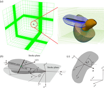
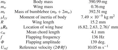
In the wing model the angle of attack of each element is calculated by identifying the direction of the velocity of each element in the wing-fixed frame of reference. This includes summation of the wing rotation relative to the stroke plane and the body motion relative to the ground. Therefore, the wing velocity and the body velocity need to be transformed into the wing-fixed frame of reference. Similarly, to calculate aerodynamic forces that act on the body, the body velocity needs to be transformed into the body-fixed frame of reference. For these purposes, let us introduce the coordinate transforms between different coordinate frames. As is shown in figure 1, we distinguish between the ground frame, the body-fixed frame, the stroke plane frame and the wing-fixed frame. Table 1 explains the notations and abbreviations used in this paper.

Figure 1.

(a) An overview of the integrated wing-body model of a bumblebee. (b) A sketch of a single wing with the definitions of wing-fixed frame $({_{w}x},{_{w}y},{_{w}z})$, stroke plane frame $({_{sp}x},{_{sp}y},{_{sp}z})$, stroke plane angle $\theta _{SP}$, positional angle $\varphi$, elevation angle $\theta$ and feathering angle $\eta$. Here $\boldsymbol {v}(r)$ represents the velocity of a blade element on the wing with the distance $r$ to the wing base and $\alpha$ represents the corresponding angle of attack. (c) A sketch of the body with the definitions of body-fixed frame $({_{b}x},{_{b}y},{_{b}z})$, ground frame $({_{g}x},{_{g}y},{_{g}z})$ and body angle $\beta$. Here $\boldsymbol {u}$ represents the velocity of the body and $\chi$ represents the corresponding angle of attack.

Table 1.

List of notations and abbreviations.

In this study the flapping wing is assumed to be flat, rigid and rotating around the wing base with respect to the stroke plane as shown in figure 1. Therefore, the wing kinematics can be defined by the given flapping angles called positional, elevation and feathering angles. The angle $\theta _{SP}$ is the stroke plane angle with respect to the horizontal plane. The ‘rotation axis’ in our terminology is the longitudinal axis of the wing. The positional angle $\varphi$ is measured between the lateral direction and the projection of the rotation axis on the stroke plane; the elevation angle $\theta$ is the deviation angle of the rotation axis from the stroke plane; the feathering angle $\eta$ is the angular displacement of the wing about the rotation axis. The coordinate transformation matrix $E_{g\rightarrow w}$ that converts a vector from the ground frame $({_gx},{_gy},{_gz})$ to the wing-fixed frame $({_wx},{_wy},{_wz})$ can be expressed as

(2.1)\begin{equation} E_{g\rightarrow w}=E_{{\theta}\rightarrow w}E_{{\varphi}\rightarrow {\theta}}E_{sp\rightarrow {\varphi}}E_{g\rightarrow sp}, \end{equation}

where

\begin{gather*} E_{g\rightarrow sp}=\begin{pmatrix} \sin\theta_{SP} & 0 & -\cos\theta_{SP}\\ 0 & 1 & 0\\ \cos\theta_{SP} & 0 & \sin\theta_{SP} \end{pmatrix},\quad E_{sp\rightarrow {\varphi}}=\begin{pmatrix} 1 & 0 & 0\\ 0 & \cos\varphi & \sin\varphi\\ 0 & -\sin\varphi & \cos\varphi \end{pmatrix},\\ E_{{\varphi}\rightarrow \theta}=\begin{pmatrix} \cos\theta & \sin\theta & 0\\ -\sin\theta & \cos\theta & 0\\ 0 & 0 & 1 \end{pmatrix},\quad E_{\theta\rightarrow w}=\begin{pmatrix} \cos\eta & 0 & -\sin\eta\\ 0 & 1 & 0\\ \sin\eta & 0 & \cos\eta \end{pmatrix}, \end{gather*}

$E_{g\rightarrow sp}$ is the coordinate transformation matrix that converts a vector from the ground frame $({_gx},{_gy},{_gz})$ to the stroke plane frame $({_{sp}x},{_{sp}y},{_{sp}z})$ which is coinciding with the wing-fixed frame when $\varphi$, $\theta$ and $\eta$ are 0, then the coordinate transformation between the stroke plane frame $({_{sp}x},{_{sp}y},{_{sp}z})$ and the wing-fixed frame $({_wx},{_wy},{_wz})$ is

(2.2)\begin{equation} E_{sp\rightarrow w}=E_{{\theta}\rightarrow w}E_{{\varphi}\rightarrow {\theta}}E_{sp\rightarrow {\varphi}}. \end{equation}

Similarly, the coordinate transformation matrix $E_{g\rightarrow b}$ that converts a vector from the ground frame $({_gx},{_gy},{_gz})$ to the body-fixed frame $({_bx},{_by},{_bz})$ can be expressed as

(2.3)\begin{equation} E_{g\rightarrow b}= \begin{pmatrix} \cos\beta & 0 & -\sin\beta\\ 0 & 1 & 0\\ \sin\beta & 0 & \cos\beta \end{pmatrix}, \end{equation}

where $\beta$ is the body angle of a modelled bumblebee. The angular velocity of the wing in the stroke plane frame is

(2.4) \begin{align} _{sp}\boldsymbol{\omega} & = \begin{pmatrix} \dot\varphi\\ 0\\ 0 \end{pmatrix}+ E_{\varphi\rightarrow\theta}'\begin{pmatrix} 0\\ 0\\ \dot\theta \end{pmatrix}+ E'_{\varphi\rightarrow\theta}E'_{\theta\rightarrow w}\begin{pmatrix} 0\\ \dot\eta\\ 0 \end{pmatrix}\nonumber\\ &= \begin{pmatrix} \dot\varphi-\sin\theta\dot\eta \\ -\sin\varphi\dot\theta+\cos\varphi\cos\theta\dot\eta \\ \cos\varphi\dot\theta+\sin\varphi\cos\theta\dot\eta \end{pmatrix}; \end{align}

thus, the angular acceleration is

(2.5)\begin{equation} _{sp}\boldsymbol{\xi}_w=\frac{\mathrm{d}{_{sp}\boldsymbol{\omega}}}{\mathrm{d}t}. \end{equation}

The representative velocity and acceleration of each blade element are defined by the velocity and acceleration sampled along the rotation axis, i.e. at points with coordinates $(0,r,0)'$ in the wing-fixed frame, as illustrated in figure 1. Thus, the representative velocity in the stroke plane frame can be expressed as

(2.6)\begin{equation} _{sp}\boldsymbol{v}(r)={_{sp}\boldsymbol{\omega}}\times\left(E'_{sp\rightarrow w}\begin{pmatrix} 0\\r\\0 \end{pmatrix}\right).\end{equation}

In addition, if the insect flies in air with a certain velocity $_{sp}\boldsymbol {v}_b$, then the absolute velocity of the wing blade element is a sum of the wing velocity relative to the body and the body velocity relative to the ground

(2.7)\begin{equation} _{sp}\boldsymbol{v}_w(r) = {_{sp}\boldsymbol{\omega}}\times\left[E'_{sp\rightarrow w}\begin{pmatrix} 0\\r\\0 \end{pmatrix}\right]+{_{sp}\boldsymbol{v}_b}; \end{equation}

thus, the acceleration is

(2.8)\begin{equation} _{sp}\boldsymbol{a}_w(r)=\frac{\mathrm{d}{_{sp}\boldsymbol{v}_w}(r)}{\mathrm{d}t}. \end{equation}

2.2. Quasi-steady model for a flapping wing

In the blade element method the wing plate is divided into a series of thin elements, like the one located at $(0,r,0)'$ as illustrated in figure 1. Each element has its velocity ((2.4) and (2.7)) and acceleration ((2.5) and (2.8)), upon which the quasi-steady model is constructed to calculate the aerodynamic force, torque and power.

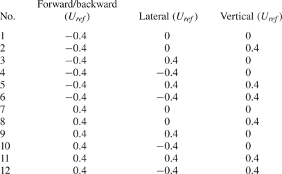
The quasi-steady model proposed in this study should give high precision for a range of velocities of the insect (forward/backward velocity, lateral velocity and vertical velocity), that is, this model should be applicable to the three-dimensional velocity space, which we define to be a cuboid ranging from $-0.4U_{ref}$ to $0.4U_{ref}$ in the forward/backward direction, $-0.4U_{ref}$ to $0.4U_{ref}$ in the lateral direction, 0 to $0.4U_{ref}$ in the vertical direction, where $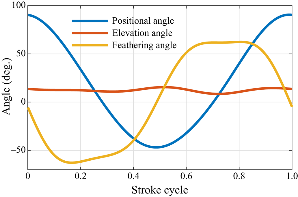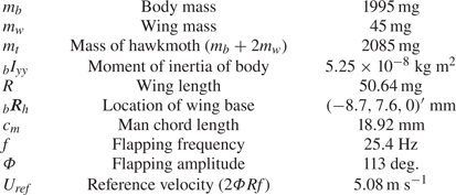U_{ref}$ is the reference velocity defined in table 2. The forward velocity can affect the lift and drag coefficients (Dickson & Dickinson Reference Dickson and Dickinson2004). The coefficients parameterizing the quasi-steady model in this paper also vary with the velocity of the modelled flying bumblebee. Thus, we construct a CFD database covering a variety of flying velocities and wing kinematics which are discrete points in the three-dimensional velocity space. The wing kinematics of hovering flight are used as a baseline in the study; see figure 2. Then the coefficients are fitted for all the discrete points separately. Finally, the interpolation method is adopted to calculate the coefficients for any point in the three-dimensional velocity space. The construction of the CFD database will be further explained in § 3.

Table 2.

Morphology of bumblebee.

Figure 2.

Wing kinematics of a hovering bumblebee (adapted from Kolomenskiy et al. Reference Kolomenskiy2019).

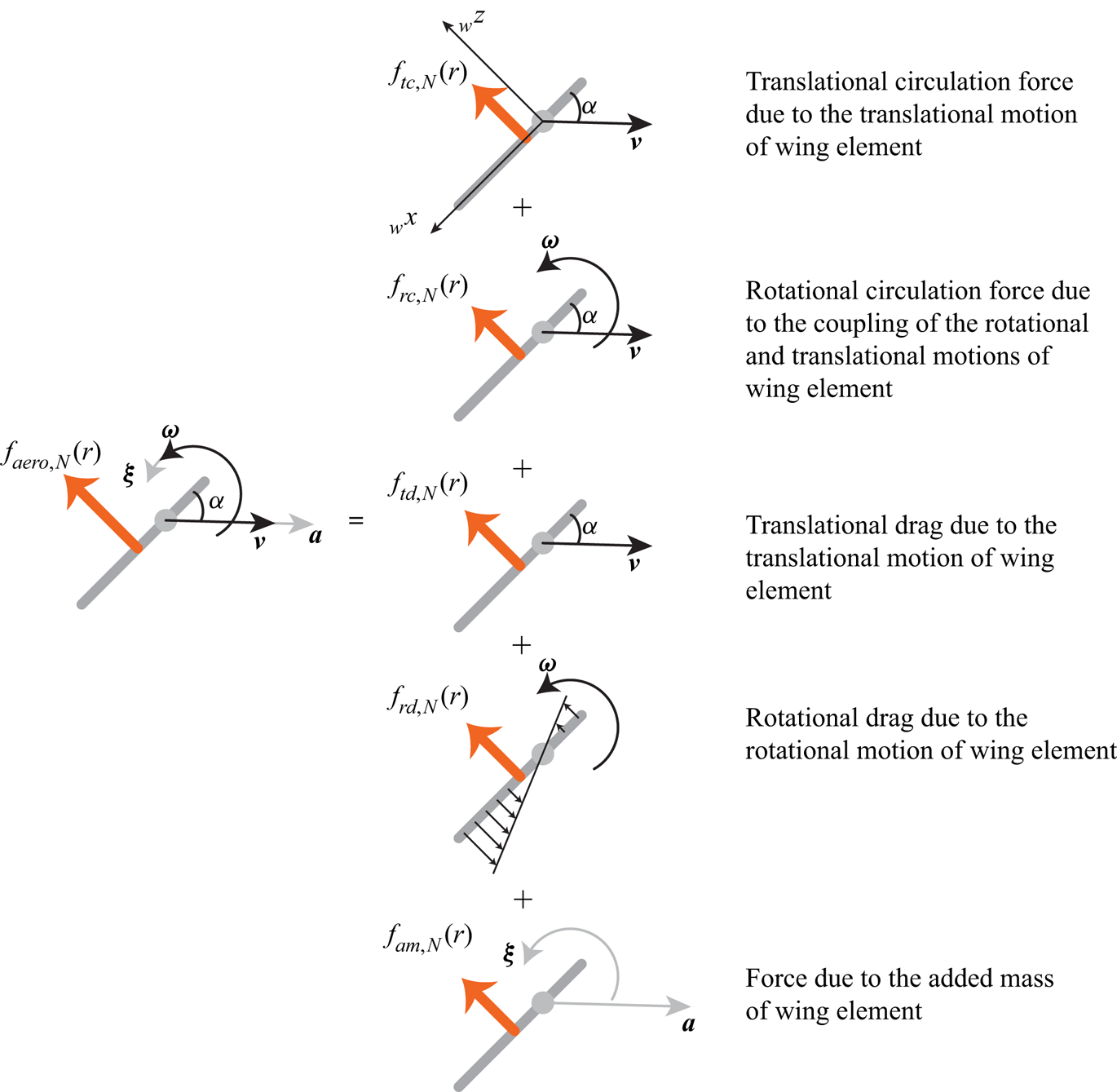
In this study the instantaneous aerodynamic force $F_{aero}$ generated by the flapping wing can be decomposed into five quasi-steady forces based on the blade element method: translational circulation force $F_{tc}$, rotational circulation force $F_{rc}$, translational drag $F_{td}$, rotational drag $F_{rd}$ and force due to added mass $F_{am}$. The CFD simulation of a flapping-wing insect has shown that the aerodynamic force applied on the flapping wing is mainly normal to the wing surface (Nakata et al. Reference Nakata, Liu and Bomphrey2015) when the Reynolds number is of the order of several hundreds or thousands because the aerodynamic force in the wings is dominated by the pressure. Therefore, the aerodynamic force is assumed to be normal to the wing surface (Sane & Dickinson Reference Sane and Dickinson2002; Wang et al. Reference Wang, Goosen and van Keulen2016; Bluman & Kang Reference Bluman and Kang2017) in this study, of which only the normal component of the instantaneous aerodynamic force is calculated as a sum of terms, i.e.

(2.9)\begin{equation} F_{aero,N}=F_{tc,N}+F_{rc,N}+F_{td,N}+F_{rd,N}+F_{am,N}. \end{equation}

Previous work on quasi-steady models mainly focused on hovering flight (Sane & Dickinson Reference Sane and Dickinson2002; Whitney & Wood Reference Whitney and Wood2010; Nakata et al. Reference Nakata, Liu and Bomphrey2015; Lee et al. Reference Lee, Lua, Lim and Yeo2016), in which the velocity of each wing blade had zero spanwise component. In our study, the absolute velocity of each wing element includes a non-zero spanwise component due to the body velocity ${\boldsymbol {v}_b}$. According to Dudley & Ellington (Reference Dudley and Ellington1990b) the spanwise component of the velocity does not contribute to the aerodynamic force production. Therefore, only the velocity component normal to the rotation axis is taken into account in the blade element method. Based on the blade element method and zero spanwise velocity assumption, the total quasi-steady aerodynamic force on a wing element is decomposed in five contributions, as shown in figure 3, and the following expressions are used to evaluate these terms (for more details, see appendix A) (Sedov Reference Sedov1965; Pesavento & Wang Reference Pesavento and Wang2004; Wang Reference Wang2004; Andersen, Pesavento & Wang Reference Andersen, Pesavento and Wang2005; Berman & Wang Reference Berman and Wang2007; Whitney & Wood Reference Whitney and Wood2010):

(2.10)\begin{gather} f_{tc,N}(r)={-}\rho c(r)C_T\cos^2\alpha|{_wv_{wn}}|{_wv_{wn,z}}, \end{gather}

(2.11)\begin{gather}f_{rc,N}(r)={-}\tfrac{1}{2}\rho C_R\dot\eta c^2(r){_wv_{wn,x}}, \end{gather}

(2.12)\begin{gather}f_{td,N}(r)={-}\tfrac{1}{2}\rho c(r)C_D\sin^2\alpha|{_wv_{wn}}|{_wv_{wn,z}}, \end{gather}

(2.13)\begin{gather}f_{rd,N}(r)={-}\tfrac{1}{6}\rho C_{rd}|\dot\eta|\dot\eta(f_l^3(r)+f_t^3(r)), \end{gather}

(2.14)\begin{gather}f_{am,N}(r)={-}A_1\frac{{\rm \pi}\rho}{4}c^2(r){_wa_{w,z}} -A_2\frac{{\rm \pi}\rho}{8}(f_l(r)+f_t(r))c^2(r){_w{\dot\omega}_{w,y}}. \end{gather}

Here $\rho$ is the density of air, $c(r)$ is the local chordwise length, $f_l$ and $f_t$ are the curves of the leading edge and trailing edge of the wing, ${{_w}v_{wn}}$ is the velocity component normal to the rotation axis of wing element, $|{_w}v_{wn}|$ represents the magnitude of ${{_w}v_{wn}}$, $C_T$ is the translational circulation coefficient, $C_R$ is the rotational circulation drag coefficient, $C_D$ is the translational drag coefficient, $C_{rd}$ is the rotational drag coefficient, $A_1$ and $A_2$ are the added mass coefficients, $\eta$ is the feathering angle, $\alpha$ is the angle of attack ranging from 0 to ${\rm \pi}$,

(2.15)\begin{equation} \alpha=\arccos\left(-\frac{_wv_{w,x}}{|{_wv}_w|}\right). \end{equation}

Hence, the total aerodynamic force on a blade element is

(2.16)\begin{equation} f_{aero,N}(r)=f_{tc,N}(r)+f_{rc,N}(r)+f_{td,N}(r)+f_{rd,N}(r)+f_{am,N}(r), \end{equation}

which can be written in summation as

(2.17)\begin{equation} f_{aero,N}(r)=\sum_{i=1}^{6}I_if_i(r), \end{equation}

where

(2.18)\begin{gather} I=[C_T,C_R,C_D,C_{rd},A_1,A_2]^\textrm{T}, \end{gather}

(2.19) \begin{gather}f(r)=\begin{pmatrix} -\rho c(r)\cos^2\alpha|{_wv_{wn}}|{_wv_{wn,z}} \\ -\frac{1}{2}\rho \dot\eta c^2(r){_wv_{wn,x}} \\ -\frac{1}{2}\rho c(r)\sin^2\alpha|{_wv_{wn}}|{_wv_{wn,z}}\\ -\frac{1}{6}\rho |\dot\eta|\dot\eta(f_l^3(r)+f_t^3(r))\\ -\dfrac{{\rm \pi}\rho}{4}c^2(r){_wa_{w,z}}\\ -\dfrac{{\rm \pi}\rho}{8}(f_l(r)+f_t(r))c^2(r){_w{\dot\omega}_{w,y}} \end{pmatrix}, \end{gather}

and the total aerodynamic forces of the wing can be obtained by integrating (2.10), (2.11), (2.12), (2.13) and (2.14) over the wing,

(2.20)\begin{equation} \left.\begin{gathered} F_{tc,N} = \int_0^Rf_{tc,N}(r)\,\mathrm{d}r,\quad F_{rc,N} = \int_0^Rf_{rc,N}(r)\,\mathrm{d}r,\quad F_{td,N} = \int_0^Rf_{td,N}(r)\,\mathrm{d}r, \\ F_{rd,N} = \int_0^Rf_{rd,N}(r)\,\mathrm{d}r,\quad F_{am,N} = \int_0^Rf_{am,N}(r)\,\mathrm{d}r, \end{gathered}\right\} \end{equation}

where $R$ is the wing length; thus, (2.9) can be written in summation as

(2.21)\begin{equation} F_{aero,N}=\sum_{i=1}^{6}I_iF_i=\sum_{i=1}^{6}I_i\int_0^Rf_i(r)\,\mathrm{d}r. \end{equation}

Figure 3.

Total aerodynamic force on a wing element can be decomposed into five quasi-steady terms.

To close the quasi-steady model for aerodynamic force, coefficients (2.18) must be determined theoretically (Sedov Reference Sedov1965; Fung Reference Fung2008), experimentally (Dickinson et al. Reference Dickinson, Lehmann and Sane1999; Sane & Dickinson Reference Sane and Dickinson2002; Andersen et al. Reference Andersen, Pesavento and Wang2005; Whitney & Wood Reference Whitney and Wood2010) or computationally (Pesavento & Wang Reference Pesavento and Wang2004; Nakata et al. Reference Nakata, Liu and Bomphrey2015; Bluman & Kang Reference Bluman and Kang2017). Nakata et al. (Reference Nakata, Liu and Bomphrey2015) identified these coefficients for hovering flight by fitting the instantaneous aerodynamic forces from a computational high-fidelity model (Liu & Kawachi Reference Liu and Kawachi1998; Liu et al. Reference Liu, Ellington, Kawachi, Van Den Berg and Willmott1998; Liu Reference Liu2009) using the least square method. A similar approach is adopted in this study. It is pointed out by Nakata et al. (Reference Nakata, Liu and Bomphrey2015) that increasing the size of input CFD database with different wing kinematics can improve the accuracy of the quasi-steady model.

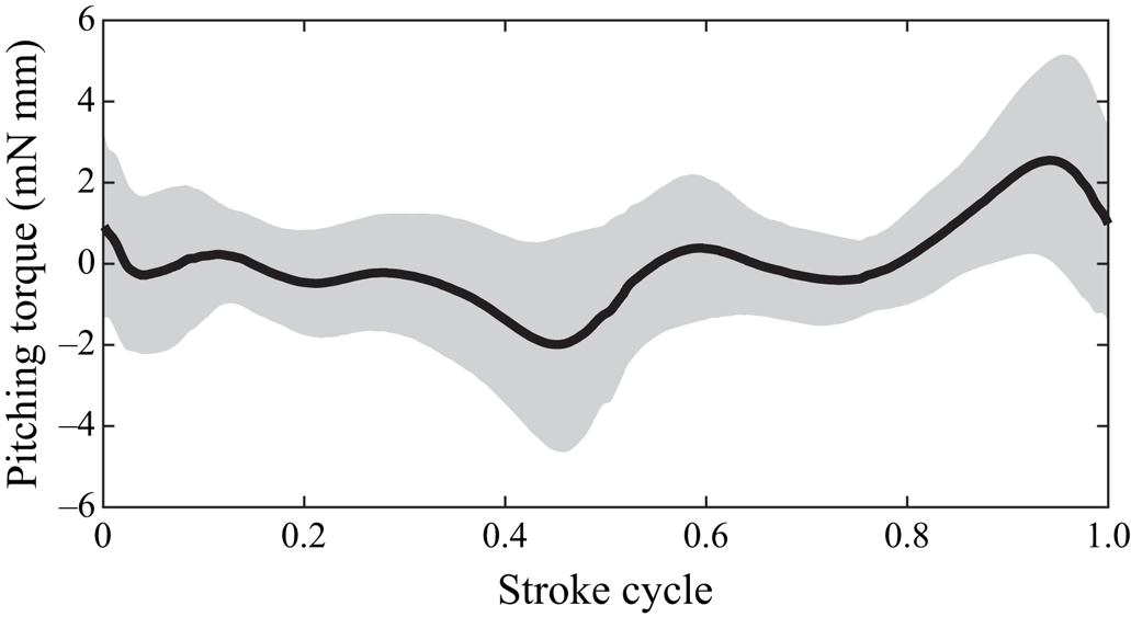
It is noted that the aerodynamic moment around the rotation axis is below 2 mN mm except for stroke reversal (below 5 mN mm); see figure 4. Following Nakata et al. (Reference Nakata, Liu and Bomphrey2015), the cycle-averaged chordwise location of aerodynamic force is fitted from the CFD simulation which is found to be only about 0.03$c_m$ away from the ‘rotation axis’, so the chordwise location of aerodynamic force is assumed to be zero. Hence, the aerodynamic torque with respect to the centre of mass of the modelled bumblebee in the body-fixed frame can be expressed as

(2.22) \begin{align} _b\boldsymbol{T}_{aero}&=\int_0^R \left[{_b\boldsymbol{R}_h}+E_{w\rightarrow b}\begin{pmatrix} 0\\r\\0 \end{pmatrix}\right]\times\left[E_{w\rightarrow b}\begin{pmatrix} 0\\0\\F_{aero,N}(r) \end{pmatrix}\right]\mathrm{d}r\nonumber\\ &={_b\boldsymbol{R}_h}\times \left[E_{w\rightarrow b}\begin{pmatrix} 0\\0\\ \displaystyle\int_0^RF_{aero,N}(r)\,\mathrm{d}r \end{pmatrix}\right]\nonumber\\ &\quad +E_{w\rightarrow b}\begin{pmatrix} \displaystyle\int_0^RrF_{aero,N}(r)\,\mathrm{d}r\\0\\0 \end{pmatrix}, \end{align}

where ${_b\boldsymbol {R}_h}$ is the position of the wing base with respect to the centre of the body in the body-fixed frame. The aerodynamic power required to move the wings through the air is

(2.23) \begin{equation} P_{aero}=\int_0^R\begin{pmatrix} 0\\0\\F_{aero,N}(r)\end{pmatrix}\cdot {_w\boldsymbol{v}_w}(r)\,\mathrm{d}r =\int_0^RF_{aero,N}(r)\cdot{_wv_{w,z}}\,\mathrm{d}r. \end{equation}

Figure 4.

Pitching torque with respect to wing hinge statistically from CFD database over one stroke cycle. Mean value (black line) $\pm$ standard deviation (shadow region).

2.3. Simplified aerodynamic model for a moving body

The contribution of a moving body to the total aerodynamic force and torque cannot be neglected. The aerodynamics of a moving insect body on its own is simpler than the unsteady aerodynamics of flapping wings. However, the interaction between the body and the wings alters the total aerodynamic performance of the body (Yu & Sun Reference Yu and Sun2009; Liu, Dong & Li Reference Liu, Dong and Li2016a). The aerodynamic force of the body fluctuates due to the reciprocating motion of the wings, and it is difficult to describe this effect by means of pure theoretical analysis. In this study we construct a simplified aerodynamic model based on the quasi-steady approximation with coefficients fitted to the CFD data. The model consists in the dynamical similarity formulae for the lift

(2.24)\begin{equation} {_b\boldsymbol{F}_{bd,L}}=\rho R^2C_{bd,L}\sin 2\chi|\boldsymbol{u}|^2(\hat{\boldsymbol{u}}\times(\hat{\boldsymbol{u}}\times {_b{\hat{\boldsymbol{x}}}})) \end{equation}

and for the drag

(2.25)\begin{equation} {_b\boldsymbol{F}_{bd,D}}={-}\rho R^2\left[C_{bd,D}(0)\cos^2\chi+C_{bd,D}\left({\frac{\rm \pi}{2}}\right)\sin^2\chi\right]|\boldsymbol{u}|^2\hat{\boldsymbol{u}}, \end{equation}

where $\hat {\boldsymbol {u}}$ is the unit vector in the direction of the body velocity, $C_{bd,L}$ is the lift coefficient, $C_{bd,D}(0)$ and $C_{bd,D}({{{\rm \pi} }/{2}})$ are the drag coefficients that correspond to the angle of attack of the body equal to 0 and ${{\rm \pi} }/{2}$, respectively. The body angle of attack $\chi$ varies between 0 and ${\rm \pi}$, and it is calculated as

(2.26)\begin{equation} \chi=\arccos\left(-\frac{_bu_{x}}{|{_bu}|}\right). \end{equation}

The direction of the lift $\boldsymbol {F}_{bd,L}$ is defined by $(\hat {\boldsymbol {u}}\times (\hat {\boldsymbol {u}}\times {_b{\hat {\boldsymbol {x}}}}))$ which is normal to the direction of the velocity $\boldsymbol {u}$. Here $\boldsymbol {F}_{bd,L}$, $\boldsymbol {u}$ and ${_b{\hat {\boldsymbol {x}}}}$ lie in the same plane; ${_b{\hat {\boldsymbol {x}}}}$ is the unit vector along the $x$ direction in the body-fixed frame. Because the aerodynamic models for the flapping wings and the moving body are independent, $C_{bd,L}$, $C_{bd,D}(0)$ and $C_{bd,D}({{{\rm \pi} }/{2}})$ are independent of wing kinematics and, in addition, are assumed to be independent of the flying velocity. Therefore, $C_{bd,L}$, $C_{bd,D}(0)$ and $C_{bd,D}({{{\rm \pi} }/{2}})$ are constants that are fitted from the CFD training database of the aerodynamic force. Because the body has bilateral symmetry, the centre of the aerodynamic force is assumed to locate on the plane of symmetry which can be expressed in the body frame as $(x_p,0,z_p)^{\prime }$. The locations $x_p$ and $z_p$ are also treated as coefficients needed to be fitted from the CFD database. The aerodynamic torque in the body frame is

(2.27)\begin{equation} {_b\boldsymbol{T}_{bd}}=\begin{pmatrix} x_p\\ 0\\ z_p \end{pmatrix}\times ({_b\boldsymbol{F}_{bd,L}}+{_b\boldsymbol{F}_{bd,D}}). \end{equation}

3. Construction of the CFD database

3.3. Computational fluid dynamics database acquisition

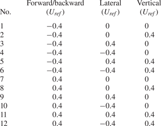
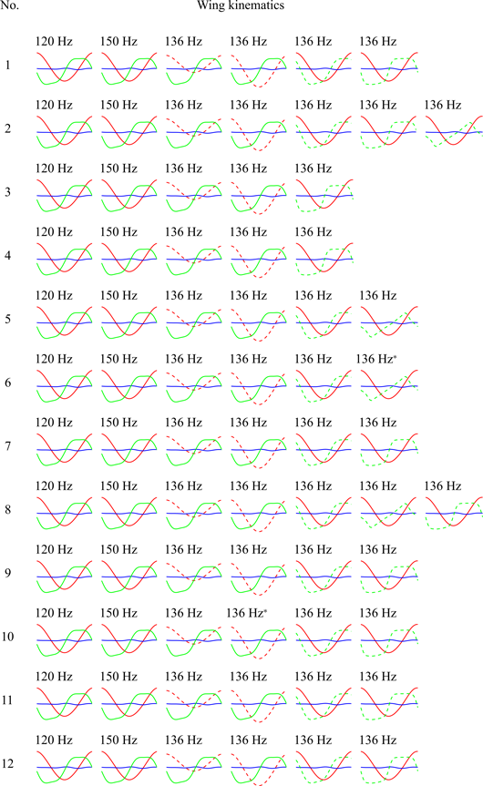
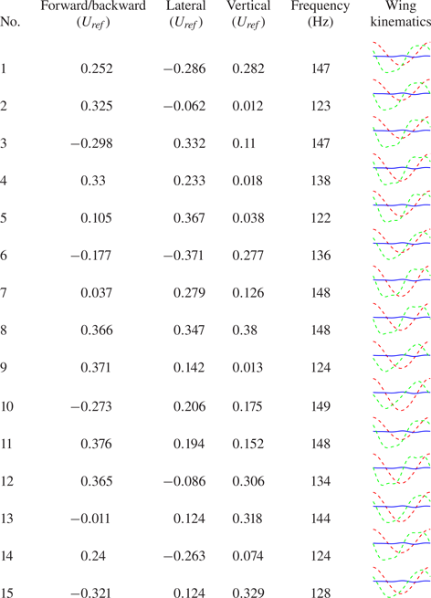
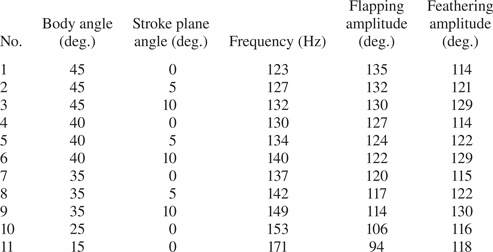
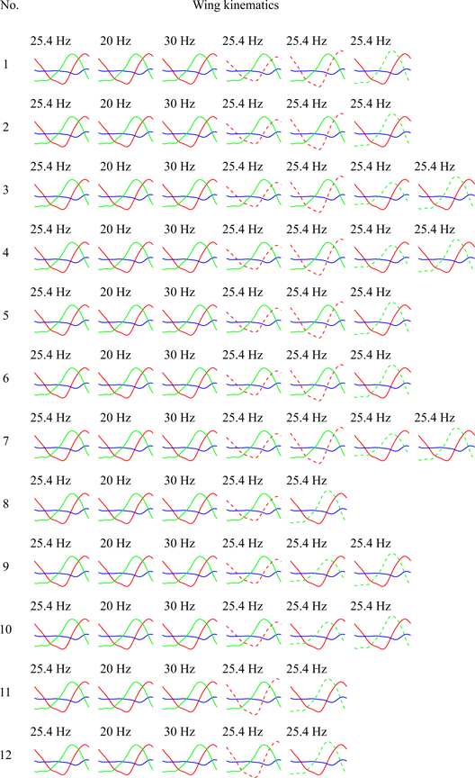
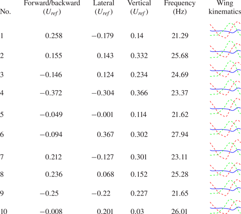
As mentioned in § 2, we ran CFD cases in different velocities; see table 3. For each velocity, several CFD cases are run with different wing kinematics; see table 4 to obtain training data. The range of wing kinematics are created by varying the wing beat frequency, as well as the positional and the feathering angle profiles. The elevation kinematics remains unchanged. A total of 71 cases are used to inform the quasi-steady model for a flapping wing and the simplified aerodynamic model for a moving body, which we denote as the training data set. To test the accuracy and generality of the quasi-steady model for flapping wings, simplified aerodynamic model for the moving body and the entire CDAM, 15 more CFD cases with randomly selected flight velocities and wing kinematics were run, forming a test data set; see table 5. Each case can be finished within 20 hours on a computer with 12 cores, hence, it takes about one month to complete the database. Online supplementary material (https://doi.org/10.1017/jfm.2021.68) includes the body grid, the wing grid along with the wing kinematics of the bumblebee model and the results (force, torque and power) of the CFD simulations.

Table 3.

Adopted flight velocities of modelled bumblebee for training data set.

Table 4.

Adopted wing kinematics of modelled bumblebee for training data set. The row numbers are corresponding to those in table 3. *Outlier of the least square error of the aerodynamic force normal to the wing surface.

Table 5.

Adopted flight velocities and wing kinematics of modelled bumblebee for test data set.

4. Coefficient fitting and accuracy testing

In this section we fit the CDAM coefficients to the CFD training data and test the performance of the model on the CFD test data.

4.1. Quasi-steady model for a flapping wing

In each CFD case the modelled bumblebee begins to flap in quiescent air and the near flow field becomes quasi-periodic after three wing beats. Therefore, for each CFD case, we select 1000 uniformly distributed points in time over the fourth cycle to fit the model coefficients of the quasi-steady model. For example, for a specified velocity $\boldsymbol {u}_{eg}$, a total of $n$ CFD cases with different wing kinematics are run. Then, a total of $1000n$ data samples of the CFD forces are selected and $1000n$ instantaneous forces of the quasi-steady model are evaluated. The least square error of the force evaluated by the quasi-steady model relative to the CFD reference data is calculated as

(4.1)\begin{align} \varepsilon_{ls}(\boldsymbol{u}_{eg}) &=\sum_{i=1}^n\sum_{k=1}^{1000}[F^i_{QSM,N}(t_k)-F^i_{CFD,N}(t_k)]^2\nonumber\\ &=\sum_{i=1}^n\sum_{k=1}^{1000}\left[\sum_{j=1}^{6}I_j(\boldsymbol{u}_{eg})F_j^i(t_k)-F^i_{CFD,N}(t_k)\right]^2, \end{align}

where $F^i_{QSM,N}(t_k)$ is the aerodynamic force normal to the wing surface calculated by (2.9) and (2.21), $F^i_{CFD,N}(t_k)$ is the aerodynamic force normal to the wing surface from the CFD simulation. Then the coefficients parameterizing the quasi-steady model for this velocity $\boldsymbol {u}_{eg}$ can be obtained by minimizing $\varepsilon _{ls}(\boldsymbol {u}_{eg})$, so called the least square method,

(4.2)\begin{align} I(\boldsymbol{u}_{eg})&= \left[\sum_{i=1}^{n}\sum_{k=1}^{1000}\begin{pmatrix} F_1^i(k)F_1^i(k) & \cdots & F_6^i(k)F_1^i(k)\\ \vdots & \ddots & \vdots\\ F_1^i(k)F_6^i(k) & \cdots & F_6^i(k)F_6^i(k)\end{pmatrix}\right]^{{-}1}\nonumber\\ &\quad \times \left[\sum_{i=1}^{n}\sum_{k=1}^{1000}\begin{pmatrix} F^i_{CFD,N}(k)F_1^i(k)\\ \vdots\\ F^i_{CFD,N}(k)F_6^i(k) \end{pmatrix}\right]. \end{align}

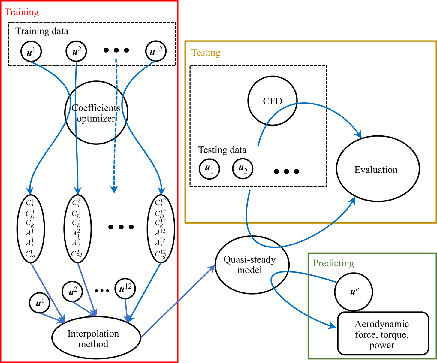
As can be seen from table 3, 12 different velocities are selected, so 12 sets of $[C_T,C_R,C_D,C_{rd},A_1,A_2]$ are fitted here. Then, an interpolation method is adopted to predict the coefficients for arbitrary velocity of the insect. We adopt the Kriging surrogate model as the interpolation method which is available as a MATLAB toolbox DACE by Lophaven et al. (Reference Lophaven, Nielsen and Søndergaard2002). The procedure is graphically illustrated in figure 5. Twelve distinct velocities as shown in table 3 and the corresponding 12 sets of fitted coefficients $[C_T,C_R,C_D,C_{rd},A_1,A_2]$ are the inputs and outputs, respectively, to inform the Kriging surrogate model.

Figure 5.

The whole procedure to construct the quasi-steady model for a flapping wing. Coefficients optimizer is formalized by (4.2) which is used to fit the coefficients of selected velocities. The interpolation method is implemented to obtain the coefficients for arbitrary flying velocity to enclose the quasi-steady model for a flapping wing which is realized by a MATLAB toolbox DACE (Lophaven, Nielsen & Søndergaard Reference Lophaven, Nielsen and Søndergaard2002). Random velocities are selected as testing data to evaluate the accuracy of the quasi-steady model by comparing the simulation results from the quasi-steady model and CFD. Thereafter, the quasi-steady model can be used to predict the aerodynamic force, torque and power of the flapping wings.

After the quasi-steady model coefficients are set, the performance of the model is evaluated on the CFD training data set and the test data set, using the least square error

(4.3)\begin{equation} \varepsilon_{ls} =\|Q_{QSM}-Q_{CFD}\|^2_2, \end{equation}

where $Q_{QSM}$ and $Q_{CFD}$ denote the aerodynamic quantities (such as aerodynamic forces, torques, power, etc.) calculated using the quasi-steady model and the CFD simulation data, respectively.

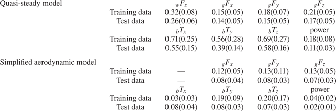
Figure 6 shows the least square error of the quasi-steady model. It can be seen that the accuracy on the test data set is well consistent with that on the training data set, which is also shown in table 6. Least square error is used to fit the coefficients, but to measure the accuracy of the quasi-steady model in practical applications like stability analysis and controller design, the cycle-averaged aerodynamic force, torque and power consumption are commonly used. Actually, the error of cycle-averaged quantities can be bounded by the least square error

(4.4)\begin{align} |\bar{Q}_{QSM}-\bar{Q}_{CFD}| &=\left|\frac{1}{1000}\sum_{i=1}^{1000}(Q^i_{QSM}-Q^i_{CFD})\right|\nonumber\\ &\le\frac{1}{1000}\sum_{i=1}^{1000}|Q^i_{QSM}-Q^i_{CFD}|\nonumber\\ &\le\sqrt{\frac{1}{1000}\sum_{i=1}^{1000}|Q^i_{QSM}-Q^i_{CFD}|^2}=\varepsilon_{ls}. \end{align}

Figure 6.

Box plots of the least square error of the quasi-steady model for a flapping wing on both the CFD training data set and test data set on the aerodynamic force normal to the wing surface and its three components in the ground frame (non-dimensionalized by $\rho U^2_{ref}c^2_m$), three components of the aerodynamic torque in the body frame (non-dimensionalized by $\rho U^2_{ref}c^3_m$) and the aerodynamic power (non-dimensionalized by $\rho U^3_{ref}c^2_m$).

Table 6.

Mean values of the least square errors of the forces (non-dimensionalized by $\rho U^2_{ref}c^2_m$), torques (non-dimensionalized by $\rho U^2_{ref}c^3_m$) and powers (non-dimensionalized by $\rho U^3_{ref}c^2_m$) for the quasi-steady model and the simplified aerodynamic model. Values in the parentheses represent the standard deviations.

Figure 7 shows the comparison of cycle-averaged aerodynamic quantities between the prediction of the quasi-steady model and CFD results. It can be seen that all the dots are close to the diagonal solid line which indicates that the predictions of the quasi-steady model approach is close to the CFD results for both the training data set and test data set. This validates the predictive capacity of the quasi-steady model. Thus, the quasi-steady model adequately approximates the aerodynamic mechanisms of flapping wings using a reduced parameter space.

Figure 7.

Comparison between the prediction of the quasi-steady model and CFD database for a flapping wing. (a–c) Aerodynamic forces in the ground frame, non-dimensionalized by $\rho U^2_{ref}c^2_m$. (d–f) Aerodynamic torques with respect to the centre of body mass of a modelled bumblebee in the body-fixed frame, non-dimensionalized by $\rho U^2_{ref}c^3_m$. (g) Aerodynamic power consumptions, non-dimensionalized by $\rho U^3_{ref}c^2_m$. Blue: training database. Red: test database. The solid line represents the equality of prediction of the quasi-steady model and CFD results.

Figures 8(a) and 8(b) show the comparison of lift and drag coefficients between the quasi-steady model and CFD results. The translational lift and drag generated by CFD simulation is obtained by subtracting the rotational circulation force, rotational drag and added mass from the force simulated by the CFD. Figure 8(c) shows the comparison of torque coefficients between the quasi-steady model and CFD results. The lift, drag and torque coefficients are defined as

(4.5)\begin{equation} C_L = \frac{2Lift}{\int_0^R{\rho cv^2\,\mathrm{d}r} },\quad C_D = \frac{2Drag}{\int_0^R{\rho cv^2\,\mathrm{d}r} },\quad C_M = \frac{2Torque}{\int_0^R{\rho crv^2\,\mathrm{d}r} }. \end{equation}

Both lift and drag coefficients of the quasi-steady model agree with CFD results well. When the angle of attack is large, the torque coefficient of the quasi-steady model is generally lower than that of CFD. This may be because of the underestimation of spanwise torque for a high angle of attack. Figures 8(d)–8(f) show the comparison between the quasi-steady model and CFD for different flight velocities. The translational lift and drag are the dominant contributors to the force generation. The rotational circulation force is also an important component for force generation, which captures the coupling effect between translation motion and rotation motion. The added mass effect plays a minor role in force generation. The contribution to vertical force of rotation drag is very small, partly because the rotation velocity peaks during the stroke reversal where the rotational drag is almost horizontal. The lift and drag coefficients for a hovering revolving wing by the proposed model is also compared with the experimental results (Usherwood & Ellington Reference Usherwood and Ellington2002), as shown in figures 8(a) and 8(b). The lift coefficient by the proposed model is almost identical to the experimental results and the proposed model overestimates the drag coefficient for an angle of attack larger than 40 degrees. This overestimation may be because the drag coefficient by the proposed model is fitted from a flapping wing rather than a revolving wing.

Figure 8.

(a) Translational lift, (b) translational drag and (c) torque coefficients for forward $0.4U_{ref}$, rightward $0.4U_{ref}$ and upward $0.4U_{ref}$ (red), forward $0.4U_{ref}$, leftward $0.4U_{ref}$ and upward $0.4U_{ref}$ (blue) and backward $0.4U_{ref}$, rightward $0.4U_{ref}$ and zero vertical speed (green). Line: quasi-steady model. Circle: CFD. The lift coefficient (a) and drag coefficient (b) for a hovering revolving wing by the present model (black line) and measured by Usherwood & Ellington (Reference Usherwood and Ellington2002) (black circles) are also shown for comparison. (d–f) Force components of the quasi-steady model in comparison with the CFD results corresponding to the three flying velocities: $(-0.4, 0.4, 0.4)U_{ref}$, $(-0.4, -0.4, 0.4)U_{ref}$ and $(0.4, 0.4, 0)U_{ref}$.

4.2. Simplified aerodynamic model for a moving body

As explained in § 2.3, five constant coefficients $[C_{bd,L},C_{bd,D}(0),C_{bd,D}({{\rm \pi} }/{2}),x_p,z_p]$ parameterizing the simplified aerodynamic model are fitted by minimizing the least square error for the CFD training data set. The results for a bumblebee are listed in table 7. Comparing the least square error of the training and the test data sets, it can be seen that the simplified aerodynamic model performs adequately; see figure 9. Compared with figure 6, the least square error in figure 9 is smaller, which demonstrates that the simplified aerodynamic model for the body is accurate enough to predict the aerodynamic force and torque of the moving body, which is also shown in table 6.

Figure 9.

Box plots of the least square error of a simplified aerodynamic model for the moving body on both the CFD training data set and testing data set. (a–c) The three components of aerodynamic force in the ground frame (non-dimensionalized by $\rho U^2_{ref}c^2_m$). (d–f) The three components of the aerodynamic torque with respect to the centre of body mass in the body frame (non-dimensionalized by $\rho U^2_{ref}c^3_m$).

Table 7.

Fitted coefficients of the simplified aerodynamic model for a moving body of a bumblebee.

Figure 10 shows the comparison of the cycle-averaged aerodynamic quantities between the simplified aerodynamic model and CFD results for the moving body. The simplified aerodynamic model performs consistently on both training data set and test data set.

Figure 10.

Comparison between the prediction of the simplified aerodynamic model and CFD database for a moving body. (a–c) Aerodynamic forces in the ground frame, non-dimensionalized by $\rho U^2_{ref}c^2_m$. (d–f) Aerodynamic torques with respect to the centre of body mass of a modelled bumblebee in the body-fixed frame, non-dimensionalized by $\rho U^2_{ref}c^3_m$. Blue: training database. Red: test database. The solid line represents the equality of prediction of the simplified aerodynamic model and CFD results.

4.3. Aerodynamic performance of the CDAM of a bumblebee

Sections 2, 4.1 and 4.2 discussed and validated the quasi-steady model for flapping wings and the simplified aerodynamic model for a moving body separately. Here, we combine them in one model, i.e. the CDAM. Figure 11 shows the comparison between the predictions using CDAM and the results of CFD simulation. The predictions by the CDAM are well consistent with the CFD results.

Figure 11.

Comparison between the prediction of the CDAM and CFD database for a bumblebee. (a–c) Aerodynamic forces in the ground frame, non-dimensionalized by $\rho U^2_{ref}c^2_m$. (d–f) Aerodynamic torques with respect to the centre of body mass of a modelled bumblebee in the body-fixed frame, non-dimensionalized by $\rho U^2_{ref}c^3_m$. (g) Aerodynamic power consumptions, non-dimensionalized by $\rho U^3_{ref}c^2_m$. Blue: training database. Red: test database. Green: trim states listed in table 8. The solid line represents the equality of prediction of the quasi-steady model and CFD results.

4.4. Discussion on the dependence of coefficients on forward flight conditions from the standpoint of fluid dynamics

The quasi-steady approach only uses the instantaneous motion of the flapping wing to predict the aerodynamic loads, while the real fluid motion around the wing has time memory. Taking hovering as an example, as shown in figure 12, compared with the first stroke cycle, the vertical force of the following stroke cycles decreases by about 15 %. This reduction is due to the existence of downwash as shown in figure 13.

Figure 12.

(a) Time course of the vertical force with the corresponding coloured dashed lines representing the peak value of the downstroke in the first stroke cycle from bottom up: hovering (0 m s$^{-1}$) and forward speed 1, 2, 3, 4 and 5 m s$^{-1}$. (b) Difference of the peak value of the vertical force in the downstroke between the first and second stroke cycle.

Figure 13.

The vertical velocity non-dimensionalized by $U_{ref}$ of the air flow on the vertical cut plane 2$c_m$ away from the sagittal plane of the bumblebee for hovering, forward speed 3 and 5 m s$^{-1}$ in the first and second stroke cycle. Red indicates the air flowing upwards and blue indicates the air flowing downwards.

Although there exist reliable downwash models for hovering flight (Oh et al. Reference Oh, Lee, Park, Choi and Kim2020), they are unlikely to generalize to arbitrary flight conditions. As shown in figure 12, the wake is almost fully developed at the second stroke cycle. The variation of the peak value during a downstroke is negative for hovering and slow forward speed 1 m s$^{-1}$ and positive for relatively fast forward speeds 2, 3, 4 and 5 m s$^{-1}$. The variation reaches maximum for medium forward velocity 2 and 3 m s$^{-1}$.

In comparison with the flapping in quiescent air during the first stroke cycle, the surrounding flow (during the second stroke cycle) induced by the previous cycle varies with the flight speed. Figure 13 shows the flow field around the mid-downstroke during the first and second stroke cycles. It can be seen that before the mid-downstroke for hovering, there exists a large area of flow with downward velocity, called downwash. When the wing encounters this downwash, the effective angle of attack decreases which causes the reduction of lift. In this study, the effect of downwash is included into the fitted coefficients. Conversely, for a forward speed of 3 m s$^{-1}$, there exists an area of flow with upward velocity, we call it upwash. During the downstroke, the wing encounters this upwash, the effective angle of attack increases which causes the rise of lift. 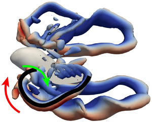For a large forward speed of 5 m s$^{-1}$, there also exists an area of flow with upward velocity, but it is weaker than that for a 3 m s$^{-1}$ forward speed, so its contribution to lift enhancement is small. To elucidate how the downwash and upwash are generated and how they interact with the flapping wing, we illustrate the vortex structure around the flying bumblebee; see figure 14. For all the three forward speeds, there is a vortex tube connecting to the wing tip behind the wing during upstroke which originates from the detached trailing edge vortex; see figure 14(a–c). The fluid flows downward through the area bounded by the vortex tube and the wing. Outside this area, the fluid flows upward. Such fluid motion is maintained by the vortex tube in the following downstroke but its interaction with the flapping wing varies with forward speed. For hovering, the downwash locates by the side of the body. This downwash interacts with the flapping wing, resulting in a reduction of force; see figure 14(d). For the forward speed 3 m s$^{-1}$, the vortex tube moves behind the bumblebee and the upwash moves to the side of the body and interacts with the flapping wing resulting in increment of force; see figure 14(e). For the forward speed 5 m s$^{-1}$, the vortex tube moves further behind the bumblebee and both the areas of downwash and upwash move behind the bumblebee, so there are almost no interactions between the downwash and/or upwash and flapping wing; see figure 14(f).

Figure 14.

Vortical structures around a flying bumblebee (isosurface with $Q=0.1$, coloured by vertical velocity non-dimensionalized by $U_{ref}$). (a,d) Hovering; (b,e) forward speed 3 m s$^{-1}$; (c,f) forward speed 5 m s$^{-1}$. Red arrows: upward flow; green arrows: downward flow. Black curve: vortex tube.

Quasi-steady models predict the aerodynamic loads only based on the instantaneous wing motion which cannot include the complex interaction of the wing and the pre-developed flows for a variety of flight speeds. By collecting a large database of CFD simulations, the coefficients parameterizing the quasi-steady model can thereby be informed to include such speed-varying flow effects. The relationship between the trained coefficients and forward velocities is illustrated by figure 15. The trained coefficients present a strong dependency on the forward velocity-related unsteady aerodynamics. Thus, the model is well trained to capture the forward-velocity-dependent unsteady aerodynamic effects compared with previous studies. For hovering, the trained translational lift coefficient $C_T$ is well consistent with that of previous work (Berman & Wang Reference Berman and Wang2007). The trained translational drag coefficient $C_D$ is comparatively larger than that of a previous study (Berman & Wang Reference Berman and Wang2007), which originates from a translational wing (Usherwood & Ellington Reference Usherwood and Ellington2002), as shown in figure 8(b). A theoretical formula for the translational drag coefficient has been provided by Wang et al. (Reference Wang, Goosen and van Keulen2016), that is, , which is equal to 3.75 for the bumblebee in this study with aspect ratio and is well consistent with the trained $C_D$ equal to 4.05. The trained rotational lift coefficient $C_R$ is comparatively larger than that with the value ${\rm \pi}$ of previous studies (Ellington & Lighthill Reference Ellington and Lighthill1984; Berman & Wang Reference Berman and Wang2007), which is theoretically derived for inviscid flows. It has been found that the theoretical $C_R$ may cause poor predictions and needs to be modified to achieve good agreements (Wang et al. Reference Wang, Goosen and van Keulen2016; Bluman & Kang Reference Bluman and Kang2017), which may explain the difference between the trained rotational lift coefficient and the theoretical one. The trained $C_{rd}$ and $A_1$ also deviate from those of a previous study, which may be because the rotational drag and added mass contribute insignificantly to the force production, as shown in figures 8(d)–8(f), and variation in the magnitudes of $C_{rd}$ and $A_1$ do not alter the force production. The feature of downwash-to-upwash transition is also well captured in terms of the rapid increase in $C_T$ and the convex-like variation in $C_R$, $C_D$, $C_{rd}$, $A_1$ and $A_2$. In conclusion, the CFD-informed method based on the solutions to the Navier–Stokes equations can assure the fundamental unsteady aerodynamics (fluid physics) associated with flapping flights in arbitrary flight velocities, which ensures the CFD-informed quasi-steady approach is capable of a fast and precise prediction of flapping aerodynamics. If the flight speed is arbitrary, the unsteady aerodynamic effects can be more complicated. With the aid of the CFD data-driven method, despite the complexity of the air flow, the quasi-steady approach is applicable to arbitrary flight speed.

Figure 15.

Variation of trained aerodynamic coefficients with forward velocity. $C_T$, $C_R$, $C_D$ (by Usherwood & Ellington Reference Usherwood and Ellington2002; Berman & Wang Reference Berman and Wang2007), $C_{rd}$, $A_1$ and $A_2$ (by Whitney & Wood Reference Whitney and Wood2010) from a previous study are shown for comparison.

5. Trim state of modelled bumblebee in forward flight

The CDAM is demonstrated to precisely predict the aerodynamic force, torque and power for a flying bumblebee with a vast range of velocity and various wing kinematics. Now, we further demonstrate the predictive capacity of CDAM by finding the trim state of a bumblebee in forward flight. In forward flight, the body posture, stroke plane and wing kinematics differ from those in hovering flight. If a bumblebee flies forward at a constant speed, its equilibrium state has to satisfy three conditions (so called trim conditions): cycle-averaged forward/backward aerodynamic force equals zero; cycle-averaged vertical aerodynamic force equals the weight of the bumblebee; cycle-averaged aerodynamic pitching moment equals zero. Here, a genetic optimization algorithm based on the derandomized evolution strategy with covariance matrix adaptation is used to find the trim state (Hansen, Müller & Koumoutsakos Reference Hansen, Müller and Koumoutsakos2003; Hansen & Kern Reference Hansen and Kern2004). The cost function is defined as

(5.1)\begin{equation} c={_g\bar{F}_x^2}+({_g\bar{F}_z}-W)^2+{_b\bar{T}_y^2}, \end{equation}

where $_g\bar {F}_x$ is the cycle-averaged forward/backward aerodynamic force, $_g\bar {F}_z$ is the cycle-averaged vertical aerodynamic force, $W$ is the weight of the bumblebee, $_b\bar {T}_y$ is the cycle-averaged aerodynamic pitching moment.

Keeping the body angle, the stroke plane angle and the forward velocity constant, we tune the wingbeat frequency, the positional angle amplitude and mean value, and the feathering amplitude and mean value. The minimal positional angle $(\varphi _{min})$ is varied to control the flapping amplitude and mean value, while the maximal positional angle $(\varphi _{max})$ remains constant during the optimization. The maximal feathering angle $(\eta _{max})$ is varied to control the feathering amplitude and mean value, while the minimal feathering angle $(\eta _{min})$ remains constant during the optimization. This is illustrated in figure 16. The genetic algorithm is used to tune the three input variables ($\,f$, $\varphi _{min}$ and $\eta _{max}$) to minimize the cost function. If the trim condition is reached, the cost function becomes zero. The initial value of the frequency is 136 Hz, the initial flapping angle amplitude is 137$^\circ$ and the initial feathering angle amplitude is 125$^\circ$. According to the measurements on the bumblebees done by Dudley & Ellington (Reference Dudley and Ellington1990a), we set the upper bound in the genetic optimization algorithm (Hansen et al. Reference Hansen, Müller and Koumoutsakos2003; Hansen & Kern Reference Hansen and Kern2004) to [175 Hz, 140$^\circ$, 140$^\circ$] and the lower bound to [120 Hz, 90$^\circ$, 100$^\circ$]. We set initial population with size 50 randomly sampled within the lower bound and upper bound. It would be prohibitively time consuming to minimize the cost function (5.1) using CFD simulation directly to calculate the aerodynamic forces and torques. Instead, we use CDAM. It took about 1000 evaluations ($\sim$10 min) to complete the optimization. Here, we focus on the flight with forward speed 1.005 m s$^{-1}$. The trim states found are listed in table 8. To check the accuracy of the trim states found by the CDAM, the predictions of both CDAM and CFD are plotted in figure 11(a,c,e,g). The agreement is satisfactory.

Figure 16.

Sketch of the extrema of wing kinematics. (a) Positional angle. (b) Feathering angle.

Table 8.

Trim states of a flying bumblebee with forward speed 1.005 m s$^{-1}$.

The solution for the trim conditions is the intersection of three isosurfaces, i.e. ${_g\bar {F}_x}=0$, ${_g\bar {F}_z}=W$ and ${_b\bar {T}_y}=0$. Here, we plot the three isosurfaces for case 6 listed in table 8 with the body angle and the stroke plane angle similar to those measured by Dudley & Ellington (Reference Dudley and Ellington1990a,Reference Dudley and Ellingtonb); see figure 17. For the isosurface ${_g\bar {F}_x}=0$, the feathering amplitude is almost constant, so the forward/backward force ${_g\bar {F}_x}$ is sensitive to the feathering amplitude and insensitive to the flapping amplitude and frequency. From the isosurface ${_g\bar {F}_z}=W$, it can be concluded that the vertical force ${_g\bar {F}_z}$ is weakly sensitive to feathering amplitude. From the isosurface ${_b\bar {T}_y}=0$, it can be concluded that the pitch torque ${_b\bar {T}_y}$ is not sensitive to the flapping frequency. To balance the pitch torque, the feathering amplitude has to be increased for smaller flapping amplitudes, and vice versa. There is only one point of intersection of the three isosurfaces, hence, there is only one solution to the trim conditions, if the body and the stroke plane angles are prescribed.

Figure 17.

Isosurface ${_g\bar {F}_x}=0$ (blue), ${_g\bar {F}_z}=W$ (red) and ${_b\bar {T}_y}=0$ (green) in the space spanned by the feathering amplitude, frequency and flapping amplitude.

More generally, from table 8, it can be seen that, for a specific forward speed, the trim state is not unique, so the bumblebee may easily reach equilibrium from an arbitrary condition. Let us consider the mass-specific aerodynamic power consumption

(5.2)\begin{equation} P^*=\frac{{power}}{m_t}. \end{equation}

We find that there is an essentially linear relationship between the body angle, the stroke plane angle and the mass-specific aerodynamic power consumption, as shown in figure 18, determined by linear regression

(5.3)\begin{equation} P^*=48.2138+0.1997(\beta - 4.5986\theta_{SP}), \end{equation}

with correlation coefficient $R^2=0.9819$. Dudley & Ellington (Reference Dudley and Ellington1990a,Reference Dudley and Ellingtonb) measured the body posture and wing kinematics of a forward flying bumblebee and estimated the power consumption. We extracted the body angle, the stroke plane angle and mean mass-specific mechanical power of three individual bumblebees from the above references and added these points on the diagram in figure 18. Although the size, mass and wing kinematics of the bumblebees measured by Dudley & Ellington (Reference Dudley and Ellington1990a,Reference Dudley and Ellingtonb) and the modelled bumblebee in this study are different, there is also a linear relationship between the mass-specific aerodynamic power and body angle and stroke plane angle. The power consumption of the three bumblebees on average is smaller than those shown in table 8. This may suggest that bumblebees prefer trim states with minimal power consumption. Combes et al. (Reference Combes, Gagliardi, Switzer and Dillon2020) studied the effect of stroke amplitude and flapping frequency on the energy cost and inferred that when carrying light loads, stability and/or maneuverability can be improved by increasing the flapping frequency which sacrifices energetic efficiency. In this study, however, for an unloaded bumblebee, power efficiency can be improved for higher flapping frequency by appropriately orienting the attitude of the insect (body angle and stroke plane angle). According to (5.3), bumblebees tend to decrease the body angle and increase the stroke plane angle to decrease the power consumption, under physiological and force generation constrains. For example, the frequency increases with the reduction of the body angle, but the bumblebee cannot increase the frequency indefinitely. We conclude that CDAM can be reliably applied to find trim states in forward flight.

Figure 18.

The linear relationship between body angle, stroke plane angle and mass-specific aerodynamic power consumption. Black line: curve of (5.3). Blue dots: trim states in table 8. Wine red dots: cases extracted from Dudley & Ellington (Reference Dudley and Ellington1990a,Reference Dudley and Ellingtonb).

6. Proportional-derivative controller design for hovering flight using CDAM

Earlier studies of the correlation between the wing kinematics and production of aerodynamic forces and torques (Hedrick & Daniel Reference Hedrick and Daniel2006; Dickinson & Muijres Reference Dickinson and Muijres2016) have enabled the development of insect-inspired flight controllers (Fei et al. Reference Fei, Tu, Zhang and Deng2019b; Yao & Yeo Reference Yao and Yeo2019; Zhang et al. Reference Zhang, Hedrick and Mittal2019). Zhang et al. (Reference Zhang, Hedrick and Mittal2019) performed costly CFD simulations to find appropriate control parameters by trial and error. Yao & Yeo (Reference Yao and Yeo2019) used a simplified aerodynamic model to derive the control parameters. However, when applied in CFD simulations, the parameters needed further adjustment.

Let us evaluate the predictive capability of CDAM from the standpoint of controller design. The CDAM can reasonably predict the aerodynamic loads on the flying bumblebee with a variety of velocities and wing kinematics which makes it suitable for control purposes. We derive a PD controller that effectively enforces longitudinal stability of the hovering bumblebee model. This methodology is applicable in forward flight. Here we apply it on the control to recover from a perturbed state (with slight forward, upward velocity and nose down pitch velocity) to hovering. The control model accounts for the sensorimotor latency. The control parameters are optimized by solving a dynamical system that encapsulates stability derivatives evaluated using CDAM. This significantly reduces the computation time compared with the trial and error method using CFD simulation. In addition, the optimized controller can be directly applied in CFD simulations because CDAM is consistent with CFD by construction.

The flight dynamics of insects is governed by rather tedious differential equations (Sun, Wang & Xiong Reference Sun, Wang and Xiong2007), if the time-accurate dynamics of flapping wings is included. However, bumblebees are heavy enough and their flapping frequency is large enough so that the fluctuation of inertial forces and torques during one period of wing beat does not influence the body dynamics on the time scale of about 10 wing beats representative of the recovery time of bumblebees after perturbation by strong wind gusts (Jakobi et al. Reference Jakobi, Kolomenskiy, Ikeda, Watkins, Fisher, Liu and Ravi2018). In this section all the quantities are expressed in non-dimensional form. Length, velocity, time, force, torque, mass, moment of inertia are non-dimensionalized by $c_m$, $U_{ref}$, $U_{ref}/c_m$, $\rho c_m^2 U_{ref}^2$, $\rho c_m^3 U_{ref}^2$, $\rho c_m^3$, $\rho c_m^5$, respectively. We therefore consider the cycle-averaged motion of the bumblebee as a solid body,

(6.1)\begin{equation} \left.\begin{gathered} {m_t}_g\dot{\bar{\boldsymbol{v}}}={_g\bar{\boldsymbol{F}}_{aero}}+m_t{_g\boldsymbol{g}},\\ {_bI}_b\dot{\bar{\boldsymbol{\omega}}}={_b\bar{\boldsymbol{M}}_{aero}}, \end{gathered}\right\} \end{equation}

where $_g\bar {\boldsymbol {v}}$ is the centre of mass velocity in the ground frame of reference and $_b\bar {\boldsymbol {\omega }}$ is the angular velocity of the body in its reference frame, dots denote time derivatives, $m_t=m_b+2m_w$ is the total mass of the bumblebee and $_bI$ is its moment of inertia. For the purpose of longitudinal control with small perturbation near hovering, (6.1) further simplify as

(6.2) \begin{equation} \begin{pmatrix} {_g\ddot{x}}\\ {_g\ddot{z}}\\ \ddot{\beta} \end{pmatrix}=\begin{pmatrix} {_g{\tilde{F}}_x}\\ {_g{\tilde{F}}_z}-g\\ {_b{\tilde{M}}_{\beta}} \end{pmatrix}, \end{equation}

where ${_g\tilde {F}_x}={_g\bar {F}_{aero,x}}/m_t$, ${_g\tilde {F}_z}={_g\bar {F}_{aero,z}}/m_t$ and ${_b\tilde {M}_{\beta }}={_b\bar {M}_{aero,y}}/_bI_{yy}$ are the cycle-averaged aerodynamic forces divided by the mass $m_t=3.92\times 10^{-4}$ kg and the aerodynamic torque divided by the moment of inertia $_bI_{yy}=7.49\times 10^{-9}$ kg m$^2$, respectively. As discussed in §§ 2 and 4, the cycle-averaged aerodynamic forces and torques can be accurately predicted by CDAM and they depend on the motion of the flying bumblebee and its wing kinematics. The wing motion should be controlled to maintain the hovering state. Here, we choose to vary the positional angle amplitude $\varDelta \varPhi$, the mean positional angle $\varDelta \bar {\varphi }$ and the mean feathering angle $\varDelta \bar {\eta }$ as control inputs; see figure 19. Hence, the quantities ${_g\tilde {F}_x}$, ${_g\tilde {F}_z}$ and ${_bM_{\beta }}$ are treated as functions of six state variables,

(6.3)\begin{equation} \left.\begin{gathered} {_g\tilde{F}_x}={_g\tilde{F}_x}({_g\dot{x}},{_g\dot{z}},\dot{\beta},\varDelta\varPhi,\varDelta\bar{\varphi},\varDelta\bar{\eta}),\\ {_g\tilde{F}_z}={_g\tilde{F}_z}({_g\dot{x}},{_g\dot{z}},\dot{\beta},\varDelta\varPhi,\varDelta\bar{\varphi},\varDelta\bar{\eta}),\\ {_b\tilde{M}_{\beta}}={_b\tilde{M}_{\beta}}({_g\dot{x}},{_g\dot{z}},\dot{\beta},\varDelta\varPhi,\varDelta\bar{\varphi},\varDelta\bar{\eta}). \end{gathered}\right\} \end{equation}

For hovering, $({_g\tilde {F}_x},{_g\tilde {F}_z},{_b\tilde {M}_{\beta }})' = (0,g,0)'$. Considering small perturbation approximation around hovering, (6.3) can be approximated by the first order of its Taylor series expansion which, after substitution into (6.2), yields the governing dynamic equation near hovering,

(6.4) \begin{equation} \begin{pmatrix} {_g\ddot{x}}\\ {_g\ddot{z}}\\ \ddot{\beta} \end{pmatrix}=D\begin{pmatrix} {_g\dot{x}}\\ {_g\dot{z}}\\ \dot{\beta} \end{pmatrix}+W\begin{pmatrix} \varDelta\varPhi\\ \varDelta\bar{\varphi}\\ \varDelta\bar{\eta} \end{pmatrix}, \end{equation}

where $D$ is the damping matrix and $W$ is the effect matrix describing the effect of wing kinematics on the acceleration of the bumblebee,

(6.5) \begin{equation} D=\left.\begin{pmatrix} \dfrac{\partial{_g\tilde{F}_x}}{\partial{_g\dot{x}}} & \dfrac{\partial{_g\tilde{F}_x}}{\partial{_g\dot{z}}} & \dfrac{\partial{_g\tilde{F}_x}}{\partial\dot{\beta}}\\ \dfrac{\partial{_g\tilde{F}_z}}{\partial{_g\dot{x}}} & \dfrac{\partial{_g\tilde{F}_z}}{\partial{_g\dot{z}}} & \dfrac{\partial{_g\tilde{F}_z}}{\partial\dot{\beta}}\\ \dfrac{\partial{_b\tilde{M}_{\beta}}}{\partial{_g\dot{x}}} & \dfrac{\partial{_b\tilde{M}_{\beta}}}{\partial{_g\dot{z}}} & \dfrac{\partial{_b\tilde{M}_{\beta}}}{\partial\dot{\beta}}\end{pmatrix}\right|_0,\quad W=\left.\begin{pmatrix} \dfrac{\partial{_g\tilde{F}_x}}{\partial\varDelta\varPhi} & \dfrac{\partial{_g\tilde{F}_x}}{\partial\varDelta\bar{\varphi}} & \dfrac{\partial{_g\tilde{F}_x}}{\partial\varDelta\bar{\eta}}\\ \dfrac{\partial{_g\tilde{F}_z}}{\partial\varDelta\varPhi} & \dfrac{\partial{_g\tilde{F}_z}}{\partial\varDelta\bar{\varphi}} & \dfrac{\partial{_g\tilde{F}_z}}{\partial\varDelta\bar{\eta}}\\ \dfrac{\partial{_b\tilde{M}_{\beta}}}{\partial\varDelta\varPhi} & \dfrac{\partial{_b\tilde{M}_{\beta}}}{\partial\varDelta\bar{\varphi}} & \dfrac{\partial{_b\tilde{M}_{\beta}}}{\partial\varDelta\bar{\eta}} \end{pmatrix}\right|_0. \end{equation}

Hedrick, Cheng & Deng (Reference Hedrick, Cheng and Deng2009) in a study of the rotational damping of a hummingbird emphasized the importance of flapping counter torque (FCT). More generally, the damping effects exist in all the six directions (forward/backward, vertical, lateral, yaw, pitch and roll) which are the diagonal elements of the damping matrix. In addition, the off-diagonal elements in $D$ can be large as the motions in all directions are coupled. Cheng et al. (Reference Cheng, Fry, Huang and Deng2010) studied fast turning maneuvers of fruit fly and pointed out that the passive aerodynamic damping due to FCT can account for a large part of the deceleration during saccades. Values of $D$ and $W$ can be directly obtained using CDAM with a finite difference method, for example, ${\partial {_g\tilde {F}_x}}/{\partial {_g\dot {x}}}\approx {({_g\tilde {F}_x}(\delta {_g\dot {x}},0,0,0,0,0)-{_g\tilde {F}_x}(0,0,0,0,0,0))}/{(\delta {_g\dot {x}})}$, with a sufficiently small $\delta {_g\dot {x}}$.

Figure 19.

Variation of wing kinematics: (a) positional angle amplitude $\varDelta \varPhi$, (b) mean positional angle $\varDelta \bar {\varphi }$ and (c) mean feathering angle $\varDelta \bar {\eta }$.

For hovering with the wing kinematics as shown in figure 2, $D$ and $W$ are expressed as

(6.6) \begin{equation} \left.\begin{gathered} D=\begin{pmatrix} -4.47 & 2.28 & -5.99\\ -0.15 & -9.37 & -0.69\\ -10.7 & 3.62 & -31.2 \end{pmatrix}\times{10}^{{-}4},\\ W=\begin{pmatrix} 0.29 & -0.45 & 6.55\\ 7.71 & 0.00 & -1.24\\ 1.66 & -7.36 & 9.84 \end{pmatrix}\times{10}^{{-}4}. \end{gathered}\right\} \end{equation}

It can be seen from $D$ that the pitch velocity has a significant effect on the forward/backward acceleration and, reversely, the forward/backward velocity also has an effect on the pitch acceleration. According to (6.4), the motion can be controlled by tuning the wing kinematics $\varDelta \varPhi$, $\varDelta \bar {\varphi }$ and $\varDelta \bar {\eta }$. Inspection of the matrix $W$ reveals that the forward/backward motion is mainly controlled by the mean feathering angle, vertical motion is mainly controlled by the amplitude of the positional angle, and the body pitching motion is sensitive to both the mean positional angle and the mean feathering angle. With an objective of implementing a practical control strategy that would enable our bumblebee model to maintain hovering, we first introduce a transformation matrix $P$ which helps to decouple the dynamical system by diagonalizing the damping matrix

(6.7)\begin{equation} PDP^{{-}1}=\varLambda=\begin{pmatrix} \lambda_1 & 0 & 0\\0 & \lambda_2 & 0\\0 & 0 & \lambda_3 \end{pmatrix}, \end{equation}

where

(6.8)\begin{equation} \lambda_1 ={-}3.2\times 10^{{-}3}, \quad \lambda_2 ={-}2.2\times 10^{{-}4}, \quad \lambda_3 ={-}9.1\times 10^{{-}4} \end{equation}

and

(6.9)\begin{equation} P = \begin{pmatrix} -0.21 & -0.93 & 0.15\\ 0.00 & 0.01 & -0.95\\ -0.98 & 0.36 & -0.28 \end{pmatrix}. \end{equation}

With a change of variables $(\xi _1, \xi _2, \xi _3)' = P ({_gx}, {_gz}, \beta )'$, (6.4) takes the form

(6.10)\begin{equation} \begin{pmatrix} \ddot{\xi}_1\\\ddot{\xi}_2\\\ddot{\xi}_3 \end{pmatrix}= \begin{pmatrix} \lambda_1\dot{\xi}_1\\\lambda_2\dot{\xi}_2\\\lambda_3\dot{\xi}_3 \end{pmatrix}+ \begin{pmatrix} \varDelta p_1\\\varDelta p_2\\\varDelta p_3 \end{pmatrix}, \end{equation}

where

(6.11)\begin{equation} \begin{pmatrix} \varDelta p_1\\\varDelta p_2\\\varDelta p_3 \end{pmatrix}= PW\begin{pmatrix} \varDelta\varPhi\\\varDelta\bar{\varphi}\\\varDelta\bar{\eta} \end{pmatrix}. \end{equation}

If, in addition, for any $i$ $(i=1,2,3)$, $\varDelta p_i$ is set to be a function of $\xi _i$ only, then the system is transformed from a MIMO (multi-input-multi-output) system into three SISO (single-input-single-output) systems.

It has been shown that insects exert control with a certain time delay (Dyhr et al. Reference Dyhr, Morgansen, Daniel and Cowan2013). Here we set the time delay to be the period of one stroke cycle $T=1/f$. The following PD feedback controller is adopted,

(6.12)\begin{equation} \varDelta p_i(t)={-}k_i[\xi_i(t-T)+\tau_i\dot{\xi}_i(t-T)],\quad i=1,2,3. \end{equation}

After substituting (6.12) into (6.10), we obtain

(6.13)\begin{equation} \ddot{\xi}_i(t)=\lambda_i\dot{\xi}_i(t)-k_i[\xi_i(t-T)+\tau_i\dot{\xi}_i(t-T)],\quad i=1,2,3. \end{equation}

The next step is to find the optimal control parameters $k_i$ and $\tau _i$ that would guarantee the fastest return to the equilibrium state. The Laplace transform on (6.13) with $\varXi _i(s)=\mathscr {L}[\xi _i(t)]$ writes as

(6.14)\begin{equation} \varXi_i(s)=\frac{\dot{\xi}_i(0)+(s-\lambda_i+k_i\tau_i\,\textrm{e}^{{-}Ts})\xi_i(0)}{s^2-\lambda_is+k_i (1+\tau_is)\,\textrm{e}^{{-}Ts}}, \quad i=1,2,3. \end{equation}

If the exponential $\textrm {e}^{-Ts}$ is approximated using the Padé approximant of order $(2, 2)$ (Franklin, Powell & Emami-Naeini Reference Franklin, Powell and Emami-Naeini2014), (6.14) reduces to a polyrational fraction with its denominator to be a biquadratic polynomial which can be simplified as a sum of four partial fractions (Franklin et al. Reference Franklin, Powell and Emami-Naeini2014). Performing the inverse Laplace transform, we obtain

(6.15)\begin{equation} \xi_i(t)=\sum_{j=1}^{4}c_{i,j}\,\textrm{e}^{p_{i,j}t},\quad i=1,2,3, \end{equation}

where $(p_{i,1},p_{i,2},p_{i,3},p_{i,4})$ are the poles (zeros of the denominator of (6.14)). Here $(c_{i,1},c_{i,2},c_{i,3},c_{i,4})$ is dependent on the initial condition. Since $\xi _i$ can grow or decay in time exponentially, the system (6.4) or (6.10) is stable if and only if the real part is negative for all poles, that is, $\mathscr {R}(p_{i,1})< 0$, $\mathscr {R}(p_{i,2})< 0$, $\mathscr {R}(p_{i,3})< 0$, $\mathscr {R}(p_{i,4})< 0$. If the system is stable, the time needed for the system to restore to equilibrium is determined by $p_{i,o}=\max \{\mathscr {R}(p_{i,1}),\mathscr {R}(p_{i,2}), \mathscr {R}(p_{i,3}),\mathscr {R}(p_{i,4})\}$ which corresponds to the slowest time decay. Hence, our goal to realize fastest return to the equilibrium reduces to finding the values of $k_i$ and $\tau _i$ that minimize $p_{i,o}$, i.e.

(6.16)\begin{equation} \min_{k_i,\tau_i}\{p_{i,o} \} ,\quad i=1,2,3, \end{equation}

which is divided into two procedures. Firstly, we approximate the denominator of (6.14) in the form

(6.17)\begin{equation} 1+k_i\frac{1+\tau_is}{s^2-\lambda_is}\frac{1-Ts/2+(Ts)^2/12}{1+Ts/2+(Ts)^2/12}=0,\quad i=1,2,3, \end{equation}

and fix $\tau _{i}$, applying the root locus method with respect to $k_i$. The root locus method is a graphical analysis that shows how the change of a parameter of a system affects the system's dynamic response. The method was first developed by Evans (Reference Evans1948) who gave rules for plotting the paths of the roots, a plot he called the root locus. The roots $(p_{i,1},p_{i,2},p_{i,3},p_{i,4})$ of (6.17) can be clearly illustrated by the locus plot which helps to find the optimized $p_{i,o}$. Secondly, we vary $\tau _i$, then the optimized $p_{i,o}$ with respect to $\tau _i$ can be obtained, which is the solution of the optimization problem (6.16). We take $i=3$ as an example to show how to solve (6.16). For a given $\tau _3$, there exist four root loci (corresponding to $p_{3,1},p_{3,2},p_{3,3},p_{3,4}$) starting from $k_3=0(\times )$ to $k_3\to +\infty (\circ )$; see figure 20. For small $\tau _3$, $p_{3,o}$ is minimized when three roots $p_{3,1},p_{3,2},p_{3,3}$ have the same real part; see figure 20(a). With the increase of $\tau _3$, $p_{3,o}$ becomes smaller until $p_{3,1},p_{3,2},p_{3,3}$ merge in one point, figure 20(b). As shown in figure 20(c) for large $\tau _3$, when two roots $p_{3,1},p_{3,2}$ meet at the same point on the real axis, $p_{3,o}$ reaches minimum. With decreasing $\tau _3$, $p_{3,o}$ becomes smaller until $p_{3,1},p_{3,2},p_{3,3}$ merge as shown in figure 20(b). Thus, the optimized $p_{3,o}$ for (6.16) is obtained. The corresponding $k_i$ and $\tau _i$ are shown in table 9 and the corresponding poles $p_{i,j}$ are shown in table 10. Combining (6.11) and (6.12) and using the definition of $\xi _i$, we obtain an explicit expression for the control strategy,

(6.18) \begin{equation} \begin{pmatrix} \varDelta\varPhi\\\varDelta\bar{\varphi}\\\varDelta\bar{\eta} \end{pmatrix}={-}W^{{-}1}P^{{-}1} \begin{pmatrix} k_1 & 0 & 0\\0 & k_2 & 0\\0 & 0 & k_3 \end{pmatrix} \left[P\begin{pmatrix} {_gx}\\ {_gz}\\\beta \end{pmatrix} + \begin{pmatrix} \tau_1 & 0 & 0\\0 & \tau_2 & 0\\0 & 0 & \tau_3 \end{pmatrix} P\begin{pmatrix} {_g\dot{x}}\\ {_g\dot{z}}\\\dot{\beta} \end{pmatrix}\right]. \end{equation}

Figure 20.

Root locus. (a) Plot for $\tau _3=80.13$. The arrows in the small figure indicate the variation of $p_{3,1}$, $p_{3,2}$ and $p_{3,3}$ with increasing $\tau _3$. Plots for (b) $\tau _3=100.13$ and (c) $\tau _3=120.13$. The arrows in the small figure indicate the variation of $p_{3,1}$, $p_{3,2}$ and $p_{3,3}$ with decreasing $\tau _3$. Here $\times$ and $\circ$ indicate that $k_3$ equals 0 and $+\infty$, respectively.

Table 9.

Optimal control parameters of PD control.

Table 10.

Poles corresponding to optimal control parameters for time delay of one stroke cycle.

To evaluate the performance of the PD control strategy derived using CDAM, we integrate it into the CFD environment and compare the results with those in the CDAM environment with the governing time-accurate dynamic equations from Sun et al. (Reference Sun, Wang and Xiong2007) embedded. We first conduct system identification (Fei et al. Reference Fei, Tu, Yang, Zhang and Deng2019a) to fine-tune the hovering wing kinematics for CDAM and for CFD. For the default wing motion shown in figure 2, CDAM and CFD produce slightly different values for the forces and torques. For that reason, free flight simulation with the default wing kinematics would slightly deviate from hovering in a CDAM environment. To eliminate this deviation, the system identification is conducted by adding small offsets to the wing kinematics, i.e. positional amplitude offset ($\delta \varPhi$), mean positional angle offset ($\delta \bar {\varphi }$) and mean feathering angle offset ($\delta \bar {\eta }$). The method to obtain the $\delta \varPhi$, $\delta \bar {\varphi }$ and $\delta \bar {\eta }$ is the one adopted in § 5. The results are $\delta \varPhi =-0.02$, $\delta \bar {\varphi }=1.71^{\circ }$ and $\delta \bar {\eta }=-0.60^{\circ }$. Then, we apply the control strategy (6.18) in both CDAM and CFD environments, with the same values of $k_i$, $\tau _i$ and $P$-matrix. The bumblebee is set in an initial state with nose up motion: $\dot {\beta }(0) = 285.52$ deg s$^{-1}$, $_gv_x(0) = 6.1$ m s$^{-1}$, $_gv_z(0) = 4.5$ m s$^{-1}$, $\beta (0) = 45$ deg, $_gx(0) = 0$ mm, $_gz(0) = 0$ mm. In the control process in the CFD environment, the bumblebee is fixed to flap its wings for three stroke cycles to make the surrounding flow fully developed. Then the bumblebee is released to perform free flying for one stroke cycle before applying control. In the control process in CDAM, the bumblebee is immediately released to perform free flying for one stroke cycle before activating the controls.

Figure 21 shows the time evolution of the position and pitch angle of the bumblebee during the recovery transition. It can be seen that the PD control strategy is successful in both the CDAM and CFD environments. The maximal values of the forward/backward position deviation and pitch angle are similar in both environments. For the vertical position, the fluctuation amplitude in CFD is larger. Note that, in the position control, the deviation during the whole control process is smaller than the mean chord length ($4.1$ mm). At the same time, deviation of pitch angle is as large as $5^{\circ }$.

Figure 21.

Longitudinal control process. (a) Position control and (b) pitch angle. Blue: vertical position; red: forward/backward position; green: pitch angle. Solid line: prediction by CFD; dashed line: prediction by the quasi-steady model; dotted line: uncontrolled. (c) Variation of wing kinematics during the control process. Red line: positional angle. Blue line: feathering angle.

It is difficult to know the exact time delay of one species. For instance, it is in the range of 2.6–6.7 ms for fruit flies’ roll control (Beatus, Guckenheimer & Cohen Reference Beatus, Guckenheimer and Cohen2015), 5–7.5 ms for blow flies (Hengstenberg et al. Reference Hengstenberg, Sandeman, Hengstenberg and Horridge1986). Here, we study the effect of time delay on the control parameters $k$ and $\tau$ and thereby the restoring time. Figure 22(a) shows that both proportion gain and differentiation gain decrease with increment of time delay. The restoring behaviour of the system is described by (6.15) of which the $p_{i,j}$ with maximal real number determines the restoring time. After $-1/p_{i,j}$ from starting, the disturbance is decreased to $1/e$ of the original disturbance. Here, we treat $-1/p_{i,j}$ as the characteristic restoring time. From figure 22(b), the characteristic restoring time rises with the increment of time delay linearly.

Figure 22.

(a) Proportion gain $k$ (blue) and differentiation gain $k\tau$ (red) over time delay. Solid line with circle: SISO system with damping effect $\lambda _1$. Dashed line with square: SISO system with damping effect $\lambda _2$. Dotted line with upper triangle: SISO system with damping effect $\lambda _3$. (b) Characteristic restoring time over time delay. Here $T$ represents the stroke period $7.35\times 10^{-3}$ s.

The smallness of the positional deviation and similarity between the trends in the two environments demonstrate the effectiveness of the PD control strategy with the parameters determined using CDAM. This leads us to a twofold conclusion. Firstly, CDAM provides an effective tool for designing controllers that can then be used in more costly, but more predictive, CFD simulations. Secondly, to some extent, CDAM can successfully replace the CFD simulation to reduce the computation time. Other more complex control strategies like fuzzy control and reinforcement learning-based control can be designed with the aid of CDAM, which may be a promising perspective for future work.

7. Computational fluid dynamics data-driven aerodynamic model on the hawkmoth manduca

The leading edge vortex is the main contributor to the force generation. It can become unstable and tends to detach from the leading edge (Liu & Aono Reference Liu and Aono2009). The shedding of the leading edge vortex in turn causes a reduction of force (Nakata et al. Reference Nakata, Liu and Bomphrey2015) and limits the accuracy of the quasi-steady model. The hawkmoth flaps its large wings at a high Reynolds number (around 6000 in hovering) which lies within the border between insects and birds. Here we apply the proposed CDAM on the hawkmoth to test its limits at high Reynolds number.

The morphology parameters of the hawkmoth are borrowed from Willmott & Ellington (Reference Willmott and Ellington1997); see table 11. Wing kinematics of the hovering hawkmoth is shown in figure 23. As mentioned in § 2, we ran CFD cases at different velocities shown in table 12 and for each velocity, several CFD cases are run with different wing kinematics as can be seen in table 13, to obtain training data. To test the accuracy and generality of the quasi-steady model for flapping wings and the simplified aerodynamic model for a moving body, 10 more CFD cases with randomly selected flight velocities and wing kinematics are run, so called test data set; see table 14. Figure 24 shows a comparison between the quasi-steady model and CFD results. Figure 25 shows a comparison between the simplified aerodynamic model and CFD results. The predictions by the proposed model agree with the CFD results qualitatively well, but the discrepancy is larger than in the bumblebee case. Figure 26 shows the aerodynamics of the wing during upstroke in hovering. A horseshoe vortex begins to form at the onset of the upstroke, however, the leading edge vortex immediately sheds from the leading edge and a new leading edge vortex begins to form, which causes a decrease of force generation. During the shedding of the first leading edge vortex and generation of the second leading edge vortex, the quasi-steady model overestimates the force production. In conclusion, the CDAM can be generalized to the hawkmoth with a small reduction in accuracy due to the unsteadiness of leading edge vortex.

Figure 23.

Wing kinematics of a hovering hawkmoth.

Figure 24.

Comparison between the prediction of the quasi-steady model and CFD database for a flapping wing. (a–c) Aerodynamic forces in the ground frame, non-dimensionalized by $\rho U^2_{ref}c^2_m$. (d–f) Aerodynamic torques with respect to the centre of body mass of a modelled hawkmoth in the body-fixed frame, non-dimensionalized by $\rho U^2_{ref}c^3_m$. (g) Aerodynamic power consumptions, non-dimensionalized by $\rho U^3_{ref}c^2_m$. Blue: training database. Red: test database. The solid line represents the equality of prediction of the quasi-steady model and CFD results.

Figure 25.

Comparison between the prediction of the simplified aerodynamic model and CFD database for a moving body. (a–c) Aerodynamic forces in the ground frame, non-dimensionalized by $\rho U^2_{ref}c^2_m$. (d–f) Aerodynamic torques with respect to the centre of body mass of a modelled hawkmoth in the body-fixed frame, non-dimensionalized by $\rho U^2_{ref}c^3_m$. Blue: training database. Red: test database. The solid line represents the equality of prediction of the simplified aerodynamic model and CFD results.

Figure 26.

Aerodynamics of a hovering hawkmoth. The blue curve indicates the first generated leading edge vortex. The green curve indicates the second generated leading edge vortex.

Table 11.

Morphology of hawkmoth.

Table 12.

Adopted flight velocities of modelled hawkmoth for training data set.

Table 13.

Adopted wing kinematics of modelled hawkmoth for training data set. The row numbers are corresponding to those in table 12.

Table 14.

Adopted flight velocities and wing kinematics of modelled hawkmoth for test data set.

8. Limitations on the current model

In § 2 we assumed that the aerodynamic force is normal to the wing surface and its centre is located on the rotation axis. We calculate the contribution of the aerodynamic force components in the wing plane for all the CFD database with various motions and wing kinematics, which turn out to be $3.5\,\% \pm 1.8\,\%$ of the total aerodynamic force, so the aerodynamic force is mainly normal to the wing surface. The aerodynamic torque with respect to the wing hinge normal to the plane is induced by the aerodynamic force components in the wing plane, so its contribution to the total aerodynamic torque is also small, about $2.8\,\%\pm 1.6\,\%$.

The spanwise aerodynamic torque, also called pitching torque, is comparatively large especially near stroke reversal as shown in figure 4. The pitching torque is due to the aerodynamic force component normal to the wing surface along with its location from the rotation axis. Dickson et al. (Reference Dickson, Straw, Poelma and Dickinson2006) experimentally found a linear relationship between the location of the aerodynamic force and the angle of attack for the fruit fly Drosophila melanogaster. According to figure 4, the pitching torque is around zero except for the stroke reversal which means the location of aerodynamic force is near the rotation axis. During stroke reversals when the angle of attack is near ${{\rm \pi} }/{2}$, the location of aerodynamic force moves away from the rotation axis, therefore, the pitching torque becomes larger. However, the stroke reversal lasts for a short time and the pitching torque changes sign during stroke reversal, so the pitching torque has a minor effect on the overall aerodynamic torque production. Hereby, in this paper, the pitching torque is not considered. It should be noted that the chordwise location of aerodynamic force affects the pitching torque around the rotation axis which does play a crucial role in analysing and designing micro air vehicles (MAVs) with passive feathering wings (Whitney & Wood Reference Whitney and Wood2010), which is not considered in this paper. In addition, for certain wings with extreme morphology, for instance, a wing with the rotation axis located on the leading edge, the pitching torque becomes non-negligible. Further work will be focused on solving this potential limitation.

The proposed model calculates the aerodynamic force for the wings and body separately. The interactions between them are not captured, which may underestimate the aerodynamic force. There are two outliers (marked in table 4) of the least square error of the force normal to the wing surface; see figure 6(a). The modelled bumblebee corresponding to the two outliers move leftward. In such case, the inflow is disturbed by the left wing and the body before it interacts with the right wing. Such an unsteady effect is not captured by the current model.