1 Introduction
Gravity currents are ubiquitous in geophysical flows. In the ocean, dense shelf water descends the continental slope over long distances toward the ocean bottom or interleaves at the level of neutral buoyancy. Along its path, ambient water is entrained, diluting the current and thus changing its dynamics and the properties of the water masses. A quantification of these dilution processes is relevant for example to understand the transport of dense water from the Antarctic shelf toward the abyssal plain, which is part of the meridional overturning circulation (Baines & Condie Reference Baines and Condie1998). Gravity currents are also important in morphodynamics, causing sediment erosion, sediment transport and creating bed forms (Garcia & Parker Reference Garcia and Parker1993; Sequeiros et al. Reference Sequeiros, Spinewine, Beaubouef, Sun, Garcia and Parker2010; Zordan et al. Reference Zordan, Juez, Schleiss and Franca2018). A knowledge of the bottom drag of developing as well as equilibrium state currents is therefore essential for understanding these transport processes.
Most laboratory experiments considered gravity currents on horizontal or constant, small slope boundaries, using lock exchange, finite volume releases or constant supply conditions (Simpson & Britter Reference Simpson and Britter1979; Britter & Linden Reference Britter and Linden1980; Simpson Reference Simpson1982; Altinakar, Graf & Hopfinger Reference Altinakar, Graf and Hopfinger1990; Cenedese & Adduce Reference Cenedese and Adduce2010; Ungarish Reference Ungarish2011). Studies of constant supply gravity currents on sloping boundaries, with slope angles varying over a large range, have focused on the normal, constant velocity state of the current (Ellison & Turner Reference Ellison and Turner1959; Britter & Linden Reference Britter and Linden1980). This state is considered to be reached at a distance from the supply of
 ${\approx}10h_{i}$
(Odier, Chen & Ecke Reference Odier, Chen and Ecke2014), where here
 $h_{i}$
is the initial depth of the current. The flow up to this equilibrium state and the dependency of the current development on initial conditions and slope angle, including the spatial development of the current due to topography changes, has received little attentions.
Pawlak & Armi (Reference Pawlak and Armi2000) considered the development region of an arrested wedge flow over a sill on slopes up to
 $14.5^{\circ }$
and found entrainment rates in the initial region two to three times larger than those known for a developed current on these slope angles. Similar results have been obtained by Odier et al. (Reference Odier, Chen and Ecke2014) for a constant inflow light gravity current moving up a sloping boundary of
 $10^{\circ }$
. It may be expected that the current development will depend on initial interfacial instability conditions in addition to the slope. However, until the paper of Negretti, Flòr & Hopfinger (Reference Negretti, Flòr and Hopfinger2017), this has been ignored. Further, excepting Negretti et al. (Reference Negretti, Flòr and Hopfinger2017), no simultaneous measurements of the bottom drag and entrainment in gravity currents on slopes considering their mutual interaction have been conducted. Gravity currents may often be in a developing state and the properties of the developed current will depend on its history i.e. interfacial entrainment and bottom drag during flow development. Field measurement by Van Haren et al. (Reference Van Haren, Gostiaux, Morozov and Tarakanov2014), in the Romanche fracture channel, clearly indicate that different initial conditions at the beginning of the slope drastically influence the further development of the current. In a recent paper Zordan, Schleiss & Franca (Reference Zordan, Schleiss and Franca2019) also point to the importance of initial conditions of turbidity current development.
Negretti et al. (Reference Negretti, Flòr and Hopfinger2017) considered only flow development of large interfacial Richardson number before moving on to concave or linear slopes. The resulting down-slope current development exhibited a behaviour completely different from that of low initial Richardson number, considered by Pawlak & Armi (Reference Pawlak and Armi2000). Three distinct development regions have been identified: (i) nearly free fall acceleration, (ii) beginning of Kelvin–Helmholtz instability (KHI) with high entrainment and related high bottom drag, (iii) subsequent collapse of KH billows and readjustment of the current to a force equilibrium. Under these conditions gravity currents, even at
 $x\approx 30h_{i}$
, (distance of experimental observation) were far from equilibrium, i.e. a normal state, constant velocity current. Similar observations have also been reported by Kostaschuk et al. (Reference Kostaschuk, Nasr-Azadani, Meiburg, Wei, Chen, Negretti, Best, Peakall and Parsons2018), which include data from numerical and laboratory studies and from field observations.
In nature, slope changes are frequent and consequently, gravity currents may often not be in a normal state, contrary to what is generally assumed to be the case (Dallimore, Imberger & Ishikawa Reference Dallimore, Imberger and Ishikawa2001; Danabasoglu, Large & Briegleb Reference Danabasoglu, Large and Briegleb2010). There is therefore sufficient motivation to clarify the effects of the flow conditions of the current at the beginning of the slope on its further development on the slope.
We present here experimental results demonstrating the dependency of initial conditions on the current development. Different flow development regimes are observed that depend on the value of an overall acceleration parameter (introduced here) which also determines the distance required to reach an equilibrium, constant velocity regime. The slope angles considered, i.e.
 $7^{\circ }$
to
 $15^{\circ }$
, are relevant for ocean applications (see also Pawlak & Armi Reference Pawlak and Armi2000) and with these small slopes we cover already the current behaviour characteristic of large slopes, expressed by a relatively large value of acceleration parameter, i.e. large velocity oscillations with large entrainment and bottom drag; when this parameter is small the approach of an equilibrium state is smooth (no velocity oscillations). We present measurements of both bottom drag and interfacial entrainment, whereas most previous studies focus on one only, because these two processes are often considered to be uncorrelated. We show here that the bottom drag is correlated with interfacial instability (interfacial entrainment) and can thus take values much larger than estimated from boundary layer considerations. For equilibrium currents a correlation between bottom drag and entrainment has been considered by Dallimore et al. (Reference Dallimore, Imberger and Ishikawa2001). Using the estimated entrainment and drag coefficient (
 $E$
and
 $c_{D}$
) we solve the governing equations reporting a good agreement with the experimental data and allowing us to predict the distance required for the current to reach the equilibrium.
The paper is organized as follows: in § 2 we present the experimental set-up, and the measurement techniques. In § 3 the initial conditions are defined and discussed. Section 4 includes the derivation of the governing equations and in § 5 we classify the different flow regimes depending on the characteristic parameters of the spatially evolving flow. Using the entrainment and drag estimated in § 6, we compare the experimental data to the numerical solution of the governing equations in § 7. Section 8 summarizes the results and includes concluding remarks.
2 Experimental procedures
2.1 Experimental set-up
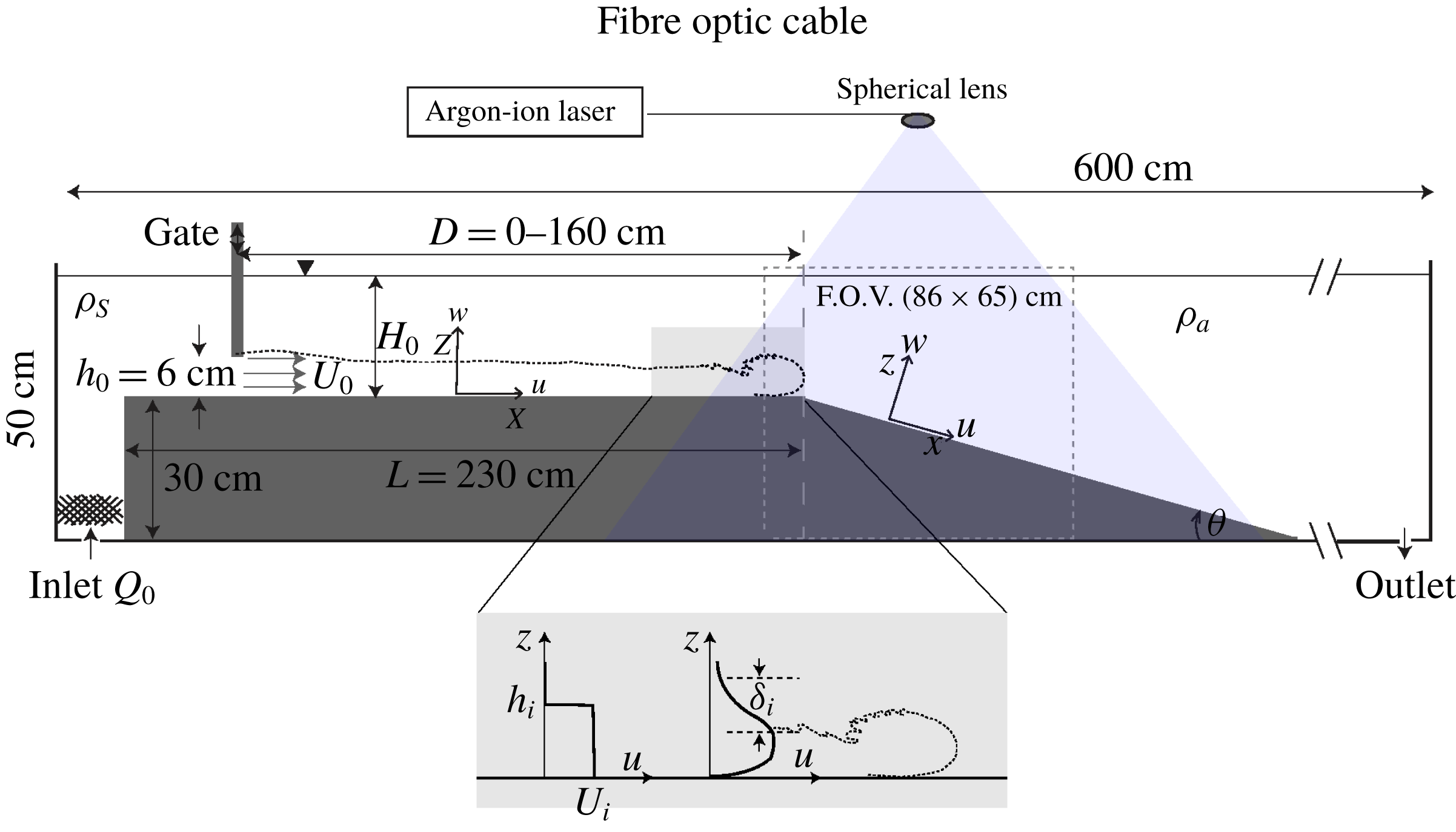
A schematic of the experimental set-up is shown in figure 1. The buoyancy driven flow has been generated using saline solutions injected at the bottom of one channel end at constant flow rate
 $Q=qb$
, via a pump, from an external
 $800$
l reservoir. The first portion of the channel is elevated by
 $30~\text{cm}$
, and is horizontal of total length of
 $L=230~\text{cm}$
and width
 $b=25~\text{cm}$
. The end of the horizontal portion is followed by a sloping boundary of slope angle
 $\unicode[STIX]{x1D703}$
on which the flow accelerates. Once the pump was switched on, the outlet at the opposing end of the tank was opened in order to enable the flow to evacuate to prevent a return flow and ensure a constant total water depth
 $H_{0}$
. The whole tank downstream of the gate was filled with fresh water with density
 $\unicode[STIX]{x1D70C}_{a}$
to a level of
 $H_{0}=18\pm 0.5~\text{cm}$
from the bottom of the elevated channel and the portion upstream of the gate was filled with salt water. The density
 $\unicode[STIX]{x1D70C}_{s}$
of the saline solution was measured just before each experiment with a densimeter (
 $\text{DMA}^{TM}35$
, Anton Paar). The experimental conditions are summarized in table 1.
Sketch of the experimental set-up.

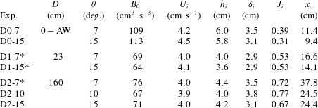
Summary of the experimental parameters (cf. figure 1 for the notations) of the particle image velocimetry (PIV) velocity measurements. The flow rate imposed by the pump was
 $Q_{p}=0.4~\text{l}~\text{s}^{-1}$
, the total water depth in the channel
 $H_{0}=(18\pm 0.5)~\text{cm}$
and the reduced gravity
 $g_{0}^{\prime }=g((\unicode[STIX]{x1D70C}_{s}-\unicode[STIX]{x1D70C}_{a})/\unicode[STIX]{x1D70C}_{a})=4.3\pm 0.1~\text{cm}~\text{s}^{-2}$
were kept equal in all the experiments.
 $D$
represents the distance of the gate from the beginning of the slope. The gate opening was
 $h_{0}=6~\text{cm}$
and was completely removed in D0 experiments (arrested wedge condition, AW). The Richardson number is
 $J_{i}=g_{0}^{\prime }\unicode[STIX]{x1D6FF}_{i}/(\unicode[STIX]{x0394}u_{i})^{2}$
.
 $h_{i}$
and
 $U_{i}$
are the current height and average velocity at 5 cm upstream of the beginning of the slope and given by the integrals (4.2.a,b
) (see figure 1). The overall and integral scale Reynolds numbers are
 $Re=uh/\unicode[STIX]{x1D708}\sim 3000$
,
 $Re_{{\mathcal{L}}}=u^{\prime 2}\sqrt{15/(\unicode[STIX]{x1D708}\unicode[STIX]{x1D716})}\sim 60$
, respectively. The field of view (FOV) was between
 $-10~\text{cm}<x<76~\text{cm}$
. In the experiments marked with an asterisk
 $\ast$
also runs with fluorescent dye (Rhodamine 6G) were conducted. The distance
 $x_{c}$
, measured from the beginning of the slope, corresponds to beginning of KHI.

The gate positions on the horizontal portion are
 $D=160~\text{cm}$
(experiments D2) and
 $D=23~\text{cm}$
(experiments D1) with gate opening
 $h_{0}=6~\text{cm}$
. A weak return flow exists of up to
 $10\,\%$
of the dense current velocity. In addition, experiments with complete removal of the gate at
 $D=5~\text{cm}$
(experiment D0) were run and were thus similar to those of Pawlak & Armi (Reference Pawlak and Armi2000), with
 $h_{0}\approx H_{0}/2$
. The return flow was in these experiments was larger, approximately
 $30\,\%$
of the dense current velocity. The slope angles were varied at
 $7^{\circ }$
,
 $10^{\circ }$
and
 $15^{\circ }$
. The depth integrated initial velocity
 $U_{i}$
, the integral current height
 $h_{i}$
(see (4.2.a,b
)) and the interface thickness
 $\unicode[STIX]{x1D6FF}_{i}$
, given in table 1, have been determined from the PIV experimental data at a distance of
 $5~\text{cm}$
upstream of the beginning of the slope (
 $x=0~\text{cm}$
) (see figure 1). The corresponding hydraulic initial conditions are expressed in terms of an initial Froude number
 $Fr^{2}={U_{i}}^{3}/B_{0}=0.94\pm 0.07$
, where
 $B_{0}=g_{0}^{\prime }q$
is the initial buoyancy flux,
 $q=U_{i}h_{i}$
is the initial flow rate per unit width and
 $g_{0}^{\prime }=((\unicode[STIX]{x1D70C}_{s}-\unicode[STIX]{x1D70C}_{a})/\unicode[STIX]{x1D70C}_{a})g$
is the initial reduced gravity.
2.2 Measurement technique
The velocities were determined using the optical, non-intrusive experimental technique of PIV. The PIV set-up consisted of a light source, light sheet optics, seeding particles, a camera and a PC equipped with a frame grabber and image acquisition software. Polyamide particles (PA12, Vestosint 1101 white) with a diameter in the range
 $d_{p}=100{-}250~\unicode[STIX]{x03BC}\text{m}$
with a specific density of
 $\unicode[STIX]{x1D70C}_{p}=1.060~\text{g}~\text{cm}^{-3}$
were added in both sides of the channel containing fresh and salt water as tracer material for the PIV measurements. It turned out that an appropriate particle density in the water body could be achieved by adding
 ${\approx}0.04~\text{g}$
particles per litre. Because of the small density difference between the two reservoirs and the given density distribution of these specific particles, it was possible to use these as seeding material for both the fresh water and the salty water. With the estimated particle time response
 $\unicode[STIX]{x1D70F}_{p}=d_{p}^{2}\unicode[STIX]{x1D70C}_{p}/18\unicode[STIX]{x1D707}\approx 4.8\times 10^{-4}$
and the Kolmogorov time scale
 $\unicode[STIX]{x1D70F}_{K}=(\unicode[STIX]{x1D708}/\unicode[STIX]{x1D716})^{0.5}\approx 0.04$
, with
 $\unicode[STIX]{x1D716}\approx {u^{\prime }}^{3}/h\approx 0.01~\text{cm}^{2}~\text{s}^{-3}$
, the Stokes number was estimated to be
 $St=\unicode[STIX]{x1D70F}_{p}/\unicode[STIX]{x1D70F}_{K}\ll 1$
thus particles are considered to follow the fluid streamlines closely.
A 6 Watt argon–ion laser (Coherent) operating in multimode (
 $\unicode[STIX]{x1D706}_{b}=488~\text{nm}$
,
 $\unicode[STIX]{x1D706}_{g}=514~\text{nm}$
) has been used as a continuous light source. The beam was transmitted through a fibre optic cable to a line generator with spherical lenses (OZ Optics Ltd., Nepean, Ontario). The generated laser sheet on the slope had a length of approximately
 $1~\text{m}$
and a width of
 $5~\text{mm}$
and was positioned in the middle of the channel.
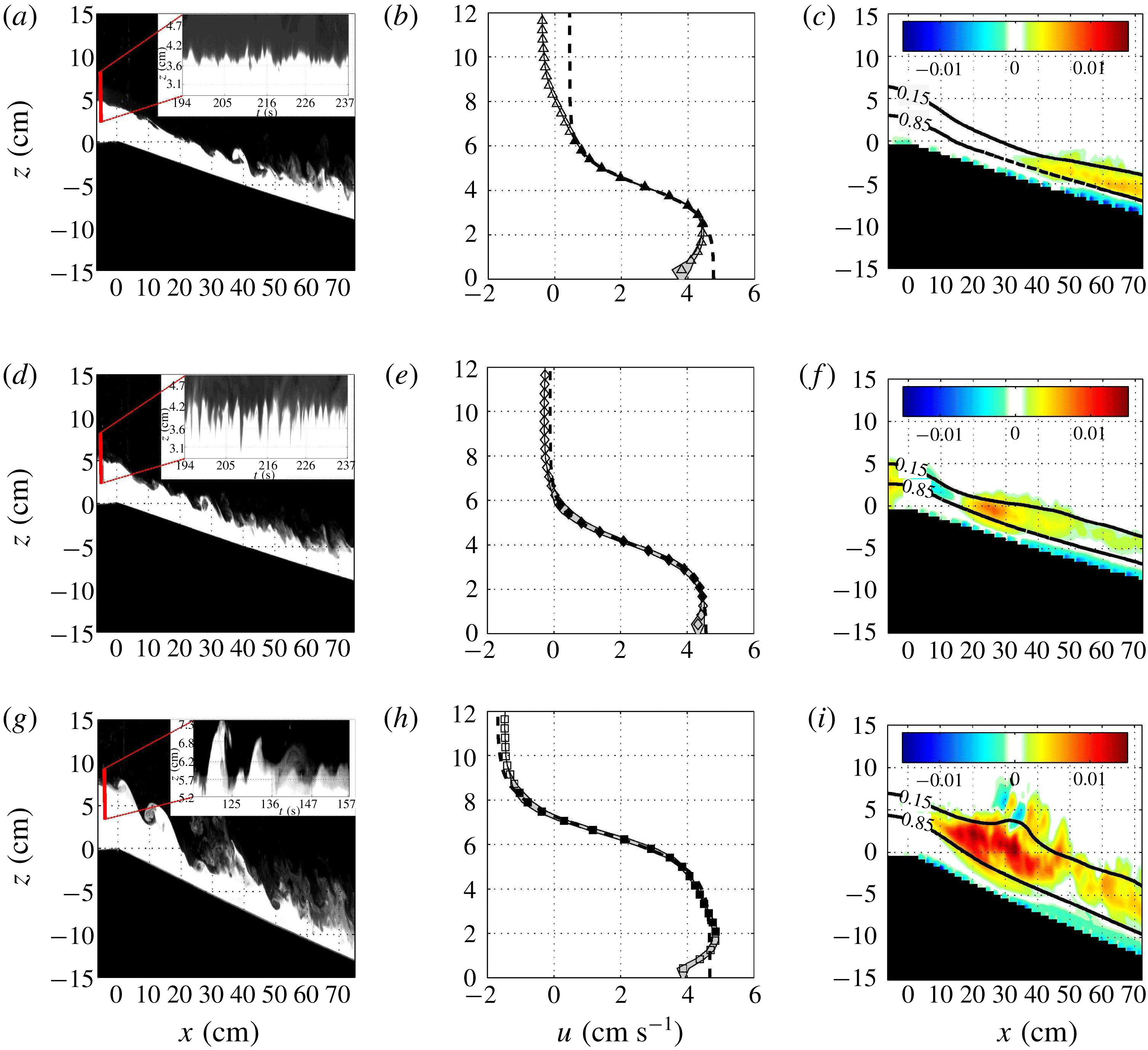
Images (a,d,g) showing dye visualization of the instantaneous gravity flow with insets showing time sequence of the density interface fluctuations 5 cm upstream of the beginning of the slope for experiments D2-7 (a), D1-7 (d) and D0-10 (g); (b,e,h), time-averaged vertical profile of streamwise velocity with experimental profile (symbols) and the confidence interval on the time average being the grey shadow; the black symbols are selected data points for the theoretical hyperbolic tangent fit (black dashed line). Images (c,f,i) show the local Reynolds stress
 $\overline{u^{\prime }w^{\prime }}/U^{2}$
with
 $85\,\%$
and
 $15\,\%$
bounds of the local maximum velocity
 $u_{m}$
contours (black continuous lines) as a measure of the shear layer thickness for experiments D2-7 (c), D1-7 (f) and D0-10 (i).

Images of
 $86~\text{cm}\times 65~\text{cm}$
were captured with a CCD camera (FlowMaster3, 14 bit,
 $1600\times 1200$
pixels) at a frame rate of
 $23.22~\text{Hz}$
and an exposure time of
 $9000~\unicode[STIX]{x03BC}\text{s}$
. A wide angle lens (SIGMA AF EX 1.8/24 DG Macro AF for Nikon) was used at a distance of
 $2~\text{m}$
to the field of view, leading to a spatial resolution of
 $0.540~\text{mm}~\text{pixel}^{-1}$
. Time series of
 $300~\text{s}$
leading to
 $7000$
raw images were stored in real time on a raid system. The raw images were then processed using a cross-correlation PIV algorithm to compute the velocity fields, each from two consecutive raw images, using the software package DaVis (LaVision). An adaptive multipass routine was used, starting with an interrogation window of
 $64\times 64$
pixels and a final window size of
 $16\times 16$
pixels with 50 % overlap. Each vector of the resulting vector field represents an area of approximately
 $0.43~\text{cm}\times 0.43~\text{cm}$
. The velocity vectors were post-processed using a local median filter and checked by the distinctiveness of the highest correlation peak. Given the velocities encountered in the experiments, the experimental error in the instantaneous velocity is estimated to be approximately
 $3\,\%$
. Further error estimations from the experiments are given in appendix A.
For dye visualizations Rhodamine 6G was added to the salt water of the gravity current with a concentration of less than
 $20~\unicode[STIX]{x03BC}\text{g}~\text{l}^{-1}$
, and they were used to estimate the density profiles and some averaged values of the density field by normalizing locally each vertical section with the maximal value.
3 Initial conditions and parameters
The initial density interface is strongly affected by the gate position and configuration. Figure 2(a,d,g) shows instantaneous images of dye visualizations with insets showing time sequences of vertical sections at
 $x=-5~\text{cm}$
highlighting interfacial density fluctuations for experiments D2-7 (a), D1-7 (d) and D0-10 (g). It is seen that the density interface fluctuations increase as the release distance (distance of gate before the beginning of the slope) is reduced: in experiments D2-7 and D1-7, the dye interface indicates the existence of Holmboe waves before the beginning of the slope, decaying in conditions D2, while for experiment D0-10 KHI appears close to the beginning of the slope.
The initial vertical profile of the streamwise velocity is also strongly affected by the gate position and configuration. Figure 2(b,e,h) shows time-averaged vertical velocity profiles, with the confidence interval on the time average (grey shadow), along with a fit with the hyperbolic tangent function (black symbols). While for experiments D1-7 (e) and D0-10 (h) the fit reproduces well the experimental profile, in experiment D2-7 (b) the fit fails in the upper part of the profile and close to the bottom. The discrepancy at the bottom is due to the development of a boundary layer on the relatively long horizontal boundary and in the outer part viscous diffusion and some mixing by Holmboe waves affect the velocity profile.
Holmboe instability (HI) is expected to exist when the velocity shear layer thickness
 $\unicode[STIX]{x1D6FF}$
is larger than the thickness of the density interface
 $\unicode[STIX]{x1D6FF}_{\unicode[STIX]{x1D70C}}$
and Hazel (Reference Hazel1972) demonstrated that HI exists at any weak shear provided
 $\unicode[STIX]{x1D6FF}/\unicode[STIX]{x1D6FF}_{\unicode[STIX]{x1D70C}}>2$
. The Holmboe instability is characterized as two sets of waves with one layer cusping into the upper layer and the other into the lower layer, and propagating in the opposite direction. The cuspids can be seen in the insets of figure 2(a,d). Theoretical studies by Haigh & Lawrence (Reference Haigh and Lawrence1999) of salinity stratified flows showed that when the bulk Richardson number
 $J$
, defined as
 $$\begin{eqnarray}J=\frac{\unicode[STIX]{x1D6FF}{g_{0}}^{\prime }}{(\unicode[STIX]{x0394}u)^{2}}\end{eqnarray}$$
is less than
 $0.071$
, KHI dominates, even when
 $\unicode[STIX]{x1D6FF}/\unicode[STIX]{x1D6FF}_{\unicode[STIX]{x1D70C}}>2$
, in agreement with the experimental findings by Koop & Browand (Reference Koop and Browand1979). Zhu & Lawrence (Reference Zhu and Lawrence2001) observed symmetric HI in the subcritical region of an exchange flow over a sill, which decayed when
 $J>0.65{-}0.75$
depending on Reynolds number. Similar results have been reported by Strang & Fernando (Reference Strang and Fernando2001) and Hogg & Ivey (Reference Hogg and Ivey2003).
To evaluate the Richardson number
 $J$
, it is necessary to measure the shear interface thickness
 $\unicode[STIX]{x1D6FF}$
. Since in the D2 experiments the velocity interface cannot be fitted by a
 $\tanh$
distribution, we determined
 $\unicode[STIX]{x1D6FF}$
by using the same method as in Pawlak & Armi (Reference Pawlak and Armi2000), i.e. the best linear fit through the normalized velocity profile between the
 $15\,\%$
and
 $85\,\%$
values,
 $$\begin{eqnarray}\unicode[STIX]{x1D6FF}=\left(\overline{\left.\frac{\unicode[STIX]{x2202}\overline{u}}{\unicode[STIX]{x2202}z}\right|_{\overline{u}(z)=0.15}^{\overline{u}(z)=0.85}}\right)^{-1},\end{eqnarray}$$
where
 $\overline{u}$
is the velocity normalized by the local velocity difference
 $\unicode[STIX]{x0394}u=u(z)|_{max}-u(z)|_{min}$
. The initial values
 $\unicode[STIX]{x1D6FF}_{i}$
are given in table 1 together with the initial Richardson number values. In experiment D2,
 $J_{i}\approx 0.72$
, the Holmboe waves are of much lower amplitude than in experiment D1 where
 $J_{i}\approx 0.53$
(figure 2
a,d,g). This agrees with the observations by Zhu & Lawrence (Reference Zhu and Lawrence2001), i.e. Holmboe waves decay when
 $J>0.7$
.
Figure 2(c,f,i) shows the change in shear layer thickness on the slope defined as the 15 %–85 % bounds of the maximum velocity
 $u_{m}$
(black continuous lines) in the downstream direction along with the Reynolds stress
 $\overline{u^{\prime }w^{\prime }}$
, which will be discussed in § 6.2.
4 Governing equations
Following the procedure of Ellison & Turner (Reference Ellison and Turner1959), Negretti et al. (Reference Negretti, Flòr and Hopfinger2017) derived the governing equations of the depth integrated velocity and density on slopes including angle variations. The assumptions made were two-dimensional stationary flow with the boundary layer and Boussinesq approximations. The
 $x$
-momentum, the mass and buoyancy flux conservation equations are
 $$\begin{eqnarray}\displaystyle & \displaystyle \frac{\text{d}U^{2}h}{\text{d}x}+\frac{1}{2}\frac{\text{d}}{\text{d}x}(S_{1}\overline{g}^{\prime }h^{2}\cos \unicode[STIX]{x1D703})=S_{2}\overline{g}^{\prime }h\sin \unicode[STIX]{x1D703}-c_{D}U^{2}, & \displaystyle\end{eqnarray}$$
 $$\begin{eqnarray}\displaystyle & \displaystyle \frac{\text{d}q}{\text{d}x}=EU, & \displaystyle\end{eqnarray}$$
 $$\begin{eqnarray}\displaystyle & \displaystyle B=\overline{g}^{\prime }q=B_{0}, & \displaystyle\end{eqnarray}$$
 $c_{D}=\unicode[STIX]{x1D70F}_{w}/\unicode[STIX]{x1D70C}U^{2}$
and
 $E$
are respectively the bottom drag and entrainment coefficients, and
 $\unicode[STIX]{x1D70F}_{w}$
the bottom shear stress,
 $\unicode[STIX]{x1D703}$
the slope angle,
 $q=Uh$
is the flow rate per unit width and
 $B=\overline{g^{\prime }}Uh$
the buoyancy flux, which is equal to the buoyancy flux supplied at the gate,
 $B_{0}$
. The parameters
 $S_{1}$
and
 $S_{2}$
are the empirical shape factors which will be discussed in more detail in appendix B. The depth integrated velocity
 $U$
, the corresponding depth
 $h$
and the depth integrated reduced gravity
 $\overline{g^{\prime }}$
are quantities defined making use of the similarity hypothesis, which implies the following relations:
 $$\begin{eqnarray}\int _{0}^{\infty }u\,\text{d}z=Uh,\quad \int _{0}^{\infty }u^{2}\,\text{d}z=U^{2}h,\end{eqnarray}$$
 $$\begin{eqnarray}\int _{0}^{\infty }g^{\prime }\,\text{d}z=S_{2}\overline{g}^{\prime }h,\quad \int _{0}^{\infty }g^{\prime }z\,\text{d}z=\frac{1}{2}S_{1}\overline{g}^{\prime }h^{2},\end{eqnarray}$$
 $x$
only. We note that the system of differential equations (4.1) reduces to a shallow water model (Ungarish Reference Ungarish2011) when fixing
 $S_{1}=S_{2}=1$
, which is equivalent to considering ‘top-hat’ density and velocity profiles.
All dimensional variables (
 $x,h,u,q$
and
 $\overline{g}^{\prime }$
), denoted below by
 $\tilde{\cdot }$
, are made dimensionless using the characteristic length and velocity scales
 ${\mathcal{L}}=(q_{0}^{2}/g_{0}^{\prime })^{1/3}={Fr_{0}}^{2/3}h_{0}\backsimeq h_{i}$
and
 ${\mathcal{U}}=(g_{0}^{\prime }q_{0})^{1/3}=\sqrt{g_{0}^{\prime }h_{0}}={Fr_{0}}^{-2/3}U_{0}\backsimeq U_{i}$
because at
 $x_{i}=-5$
cm,
 $Fr_{i}\backsimeq 1$
, i.e.
 $$\begin{eqnarray}\{\{x,h\},u,q,\overline{g}^{\prime }\}=\{{\mathcal{L}}\{\tilde{x},\tilde{h}\},{\mathcal{U}}\tilde{u} ,q_{0}\tilde{q},g_{0}^{\prime }\tilde{\overline{g}}^{\prime }\}.\end{eqnarray}$$
Equations (4.1) represent a system of three differential equations with the unknown variables
 $U$
,
 $h$
,
 $\overline{g^{\prime }}$
and can be combined and rewritten to finally give
 $$\begin{eqnarray}\frac{\text{d}\tilde{q}\tilde{U} }{\text{d}\tilde{x}}+\frac{1}{2}\frac{\text{d}}{\text{d}\tilde{x}}\left(S_{1}\frac{\tilde{q}}{\tilde{U} ^{2}}\cos \unicode[STIX]{x1D703}\right)=S_{2}\frac{1}{\tilde{U} }\sin \unicode[STIX]{x1D703}-c_{D}\tilde{U} ^{2}.\end{eqnarray}$$
Equation (4.4) can be solved numerically provided the entrainment law
 $E=E(x)$
and the variation of the bottom friction coefficient
 $c_{D}=c_{D}(x)$
are known functions of
 $x$
. Note that
 $c_{D}$
is of order
 $E$
and cannot be neglected (Negretti et al.
Reference Negretti, Flòr and Hopfinger2017; Kostaschuk et al.
Reference Kostaschuk, Nasr-Azadani, Meiburg, Wei, Chen, Negretti, Best, Peakall and Parsons2018).
As outlined in Negretti et al. (Reference Negretti, Flòr and Hopfinger2017), when the Richardson number at the beginning of the slope is large,
 $J_{i}\approx 1$
, the interface is KH stable at the beginning of the slope and in the initial acceleration region, up to
 $x_{c}$
,
 $E=c_{D}\approx 0$
. In this case (4.4) can be simplified to
 $$\begin{eqnarray}\frac{\text{d}}{\text{d}\tilde{x}}\left(\tilde{U} +\frac{1}{2}S_{1}\frac{1}{\tilde{U} ^{2}}\cos \unicode[STIX]{x1D703}\right)=S_{2}\frac{1}{\tilde{U} }\sin \unicode[STIX]{x1D703},\end{eqnarray}$$
which has the implicit solution
 $$\begin{eqnarray}\tilde{U} ^{2}+S_{1}\frac{2}{\tilde{U} }\cos \unicode[STIX]{x1D703}=C_{0}+2S_{2}\tilde{x}\sin \unicode[STIX]{x1D703}.\end{eqnarray}$$
The integration constant
 $C_{0}=(1+2S_{1}\cos \unicode[STIX]{x1D703})$
is determined imposing the initial condition
 $\tilde{U} =\tilde{U} _{i}$
, for
 $\tilde{X}=0$
and assuming the hydraulic condition at the beginning of the slope for the Froude number
 $Fr=1$
. We point out that (4.6) differs from the free fall solution presented in Negretti et al. (Reference Negretti, Flòr and Hopfinger2017) by the pressure term multiplied by
 $S_{1}$
. The different theoretical solutions and their comparison with experiments will be presented and discussed in § 7.
5 Flow development regimes
In this section time-averaged quantities are presented. For each experiment, all values have been averaged in time by taking into account only the steady layer flow (after the current head has passed). A moving averaging filter of spatial width
 ${\mathcal{L}}$
is applied and data are sub-sampled with the same spatial scale to improve the clarity of the figures. A detailed estimation of the errors is given in appendix A.
Dimensionless time-averaged velocities
 $U/U_{i}$
and current heights
 $h/h_{i}$
as a function of
 $x/h_{i}$
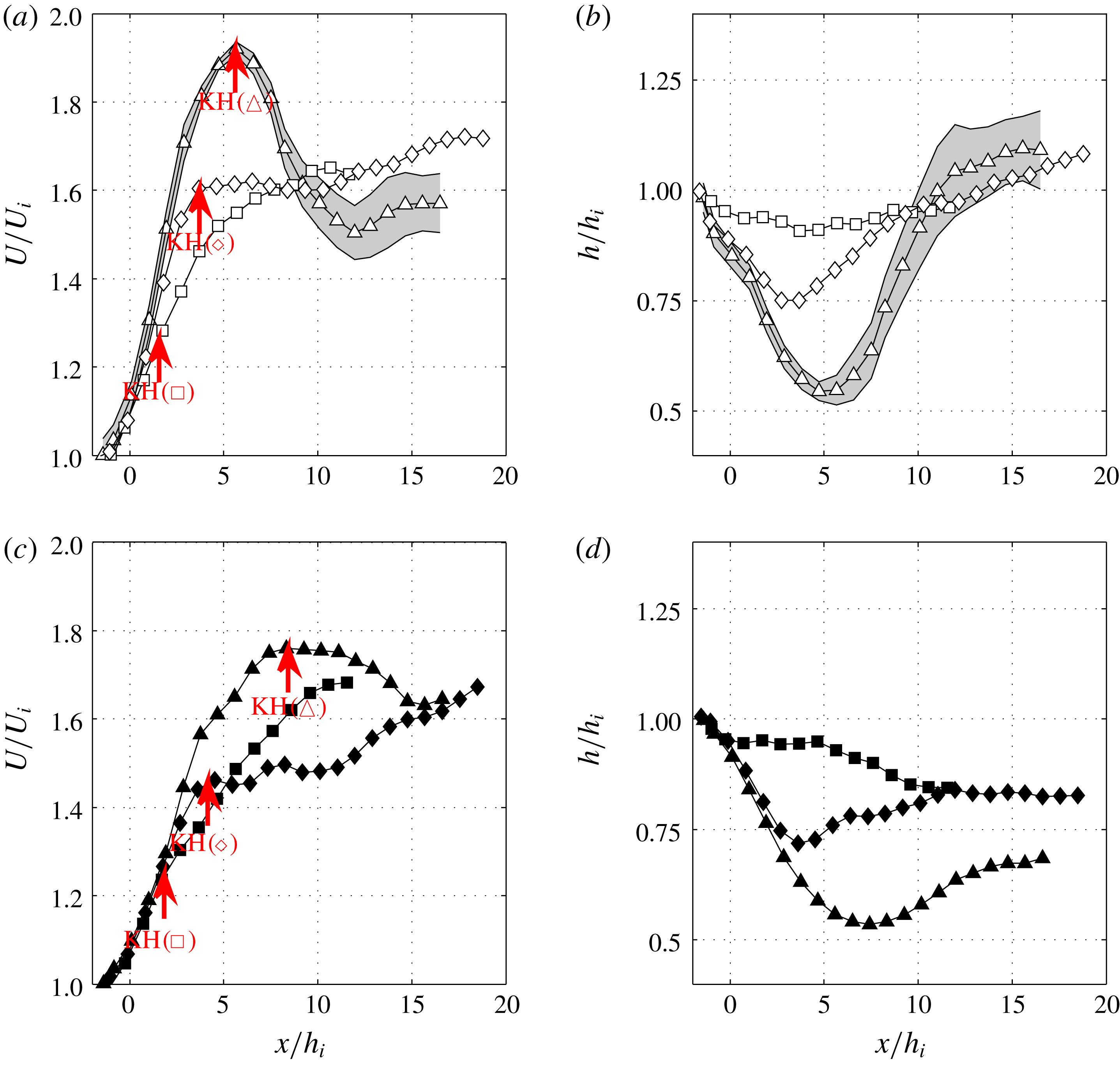
are presented in figures 3(a,c) and 3(b,d), respectively for experiments at
 $\unicode[STIX]{x1D703}=15^{\circ }$
(a,b) and
 $7^{\circ }$
(c,d). Different symbols and grey scales correspond to the release distances (D2, ▵; D1, ♢; D0, ▫). The grey shades in figure 3(a,b) represent the confidence interval of the time-averaged velocities. Figure 3(a,c) shows that in experiments D2 and D1, a strong acceleration of the current occurs until a certain distance,
 $x_{c}$
. At this position, in D2 (▵) experiments, the current velocity reaches a maximum and then decreases rapidly, whereas in D1 (♢) experiments, an abrupt change in velocity increase occurs at
 $x_{c}$
. In D0 (▫) conditions, only a small change in velocity increase at
 $x_{c}$
is observed. This critical position
 $x_{c}$
corresponds to beginning of KHI, as already observed by Negretti et al. (Reference Negretti, Flòr and Hopfinger2017), and is marked by vertical arrows in figure 3(a,c). They vary from
 $x_{c}/h_{i}\approx 6{-}8$
(15 and
 $7^{\circ }$
respectively) in D2 experiments, to
 $x_{c}/h_{i}\approx 4$
in D1 experiments and to
 $x_{c}/h_{i}\approx 2$
in D0 experiments. Similar considerations hold for the current height
 $h$
(figure 3
b,d): a strong decrease until a minimum at
 $x_{c}/h_{i}$
is observed in experiments D2 and D1, while in the D0 configuration the depth of the current remains nearly constant over the full measured domain.
Time-averaged depth integrated velocity
 $U/U_{i}$
(a,c) and height
 $h/h_{i}$
(b,d) of the gravity current as a function of
 $x/h_{i}$
for a slope of
 $15^{\circ }$
(empty symbols) (a,b), and
 $7^{\circ }$
(filled symbols) (c,d). D0 (▫, ▪), D1 (♢, ♦) and D2 (▵, ▴). The grey shade represents the confidence interval on the time average for experiment D2-15.
 $U_{i}$
and
 $h_{i}$
are initial velocity and current height
 $5$
cm upstream of the start of the slope.

Overall Richardson number
 $J$
as a function of
 $x/h_{i}$
for
 $15^{\circ }$
(empty symbols) (a) and
 $7^{\circ }$
(filled symbols) (b) and D0 (▫, ▪), D1 (♢, ♦) and D2 (▵, ▴). Arrows indicate KHI beginning. (c) Critical Richardson number
 $J_{c}$
as a function of interface thickness
 $\unicode[STIX]{x1D6FF}$
over the height
 $h$
at
 $x=x_{c}$
. D0 (▫, ▪), D1 (♢, ♦) and D2 (▵, ▴ (grey), ▴). From black to white:
 $\unicode[STIX]{x1D703}=7^{\circ },10^{\circ },15^{\circ }$
. Experimental results from Negretti et al. (Reference Negretti, Flòr and Hopfinger2017) for the gate configuration D2 and a linear slope of
 $\unicode[STIX]{x1D703}=22^{\circ }$
(
 $+$
), and two concave slopes of initial
 $\unicode[STIX]{x1D703}_{i}$
 $31.5^{\circ }$
(
 $\ast$
) and
 $17^{\circ }$
(
 $\times$
) are also included.

From these results it is clear that the conditions at the beginning of the slope strongly affect the development of the flow on the slope. As already mentioned in § 3, the current released far upstream from the slope (D2 experiments) has a large interfacial Richardson number
 $J_{i}\approx 0.67{-}0.77$
(cf. table 1) at the beginning of the slope, implying that the Holmboe waves, that are present some distance downstream of the gate, are decaying (Zhu & Lawrence Reference Zhu and Lawrence2001). When the gate is closer to the beginning of the slope, the initial Richardson number is
 $J_{i}=0.53$
(D1 experiments) and the interface remains Holmboe unstable at the beginning of the slope. In the D0 experiment,
 $J_{i}\approx 0.3$
and the current is KH unstable shortly after the beginning of the slope. Also, the effect of the slope is evident. In general, larger slopes generate larger changes in velocity and depth of the current, while on the smallest slope,
 $7^{\circ }$
, the change in velocity is smoother.
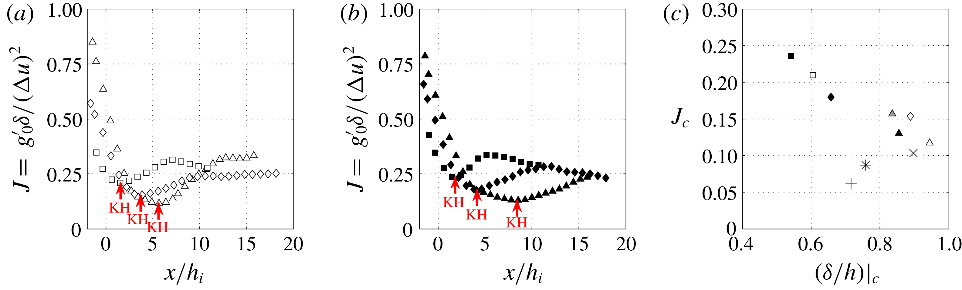
Figure 4 gives the variation of
 $J$
as a function of
 $x/h_{i}$
for the experiments of slopes
 $15^{\circ }$
(a) and
 $7^{\circ }$
(b). Again, the different symbols correspond to the different release distances (D2, ▵; D1, ♢; D0, ▫). It is seen that the larger is
 $J_{i}$
, the lower is the critical value of the Richardson number:
 $J_{c}\approx 0.24$
for D0,
 ${\approx}0.2$
for D1 and
 ${\approx}0.13$
for D2.
Onset of KHI depends on the ratio
 $\unicode[STIX]{x1D6FF}/\unicode[STIX]{x1D6FF}_{\unicode[STIX]{x1D70C}}$
and on the wall proximity, expressed by
 $(\unicode[STIX]{x1D6FF}/h)_{c}$
. As has been shown by Hazel (Reference Hazel1972), the critical Richardson number
 $J_{c}$
decreases with increasing ratio
 $\unicode[STIX]{x1D6FF}/h$
, as evident from figure 4(c) from our experiments. In the D2 experiments,
 $J_{i}$
is large (weak Holmboe wave mixing) and
 $(\unicode[STIX]{x1D6FF}/h)_{c}\approx 1$
, hence a low value of
 $J_{c}$
and the current will accelerate over a longer distance to reach this value. In the D1 experiment
 $(\unicode[STIX]{x1D6FF}/h)_{c}<1$
and Holmboe waves are more intense and can mix the density interface so that
 $\unicode[STIX]{x1D6FF}/\unicode[STIX]{x1D6FF}_{\unicode[STIX]{x1D70C}}\longrightarrow 1$
, hence a larger value of
 $J_{c}$
is expected. In the D0 experiment
 $J_{c}\approx 0.24$
because
 $\unicode[STIX]{x1D6FF}/\unicode[STIX]{x1D6FF}_{\unicode[STIX]{x1D70C}}\approx 1$
and
 $(\unicode[STIX]{x1D6FF}/h)_{c}\approx 0.5$
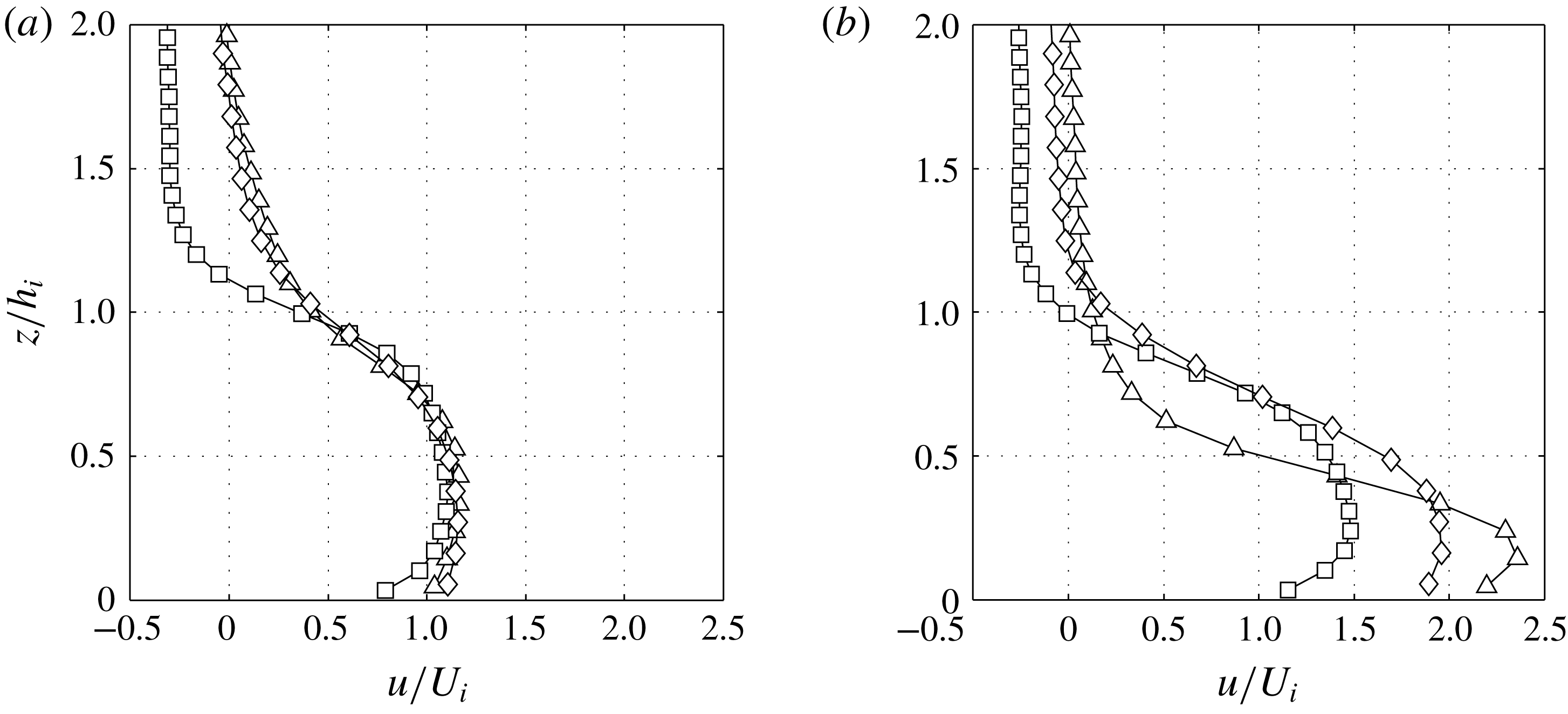
. Figure 5 shows the normalized velocity profiles
 $u/U_{i}$
before the beginning of the slope at
 $x=-5~\text{cm}$
(a) and at the location of minimum Richardson number, at
 $x_{c}$
for slope angle
 $15^{\circ }$
(b). At the beginning, the velocity profiles are similar (with the exception of the D0 experiment, which has a larger return flow–lock exchange effect), but at the location of minimum Richardson number, the velocity maximum of D2 experiment is much closer to the bottom boundary. In experiments D1 and D0 the thickness of uniform velocity is much larger. The variation of the ratio
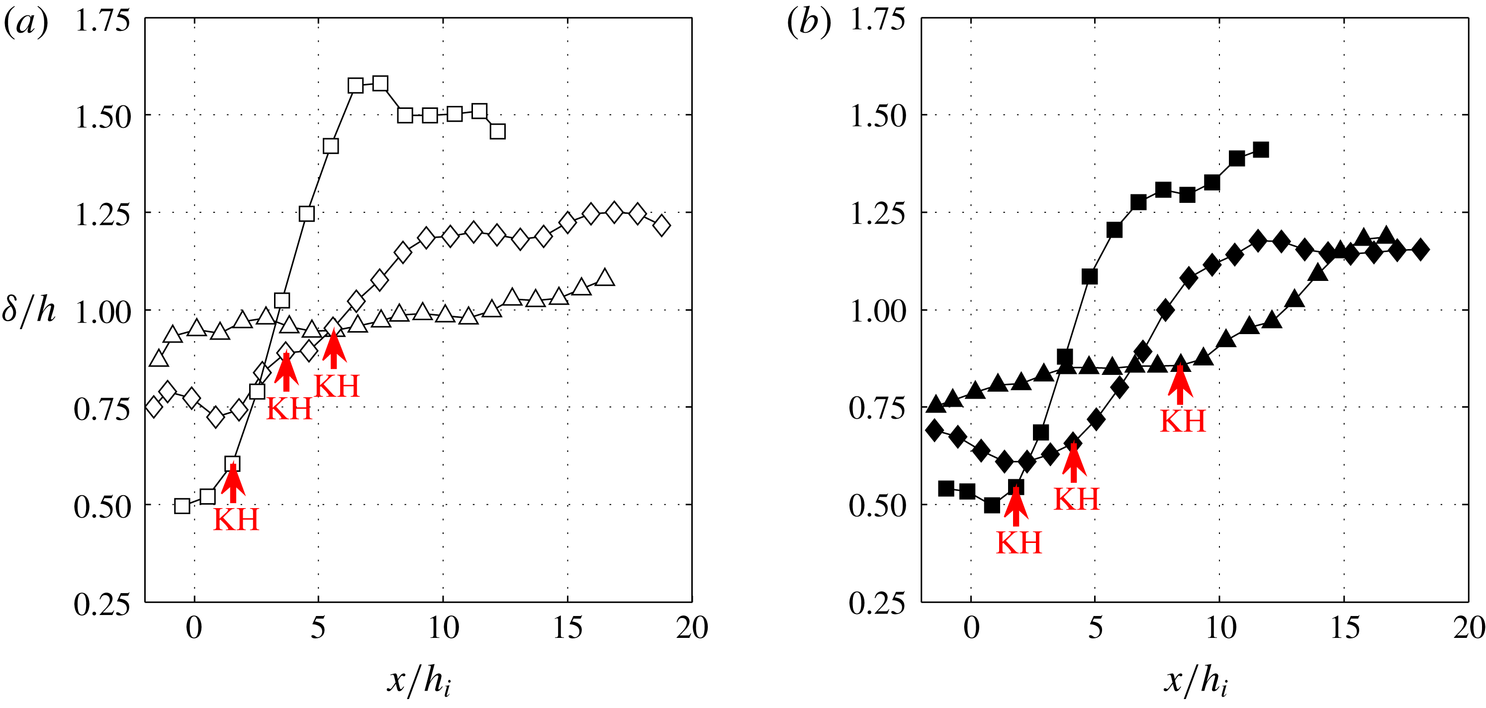
 $\unicode[STIX]{x1D6FF}/h$
is shown in figure 6 for experiments with
 $15^{\circ }$
(a) and
 $7^{\circ }$
(b). In the D0 and D1 experiments
 $\unicode[STIX]{x1D6FF}/h\lesssim 1$
, while in experiments D2,
 $\unicode[STIX]{x1D6FF}/h\approx 1$
. In the latter, the KH billows are thus larger and closer to the wall, causing boundary layer separation and large
 $c_{D}$
, as has been shown by Negretti et al. (Reference Negretti, Flòr and Hopfinger2017).
Time-averaged vertical velocity profile
 $u/U_{i}$
at
 $x=-5~\text{cm}$
(a) and
 $x=x_{c}$
(b). For
 $\unicode[STIX]{x1D703}=15^{\circ }$
. D2 (▵), D1 (♢), D0 (▫).

Ratio of shear layer thickness to current height
 $\unicode[STIX]{x1D6FF}/h$
as a function of
 $x/h_{i}$
.
 $15^{\circ }$
(empty symbols) (a) and
 $7^{\circ }$
(filled symbols) (b). D0 (▫, ▪), D1 (♢, ♦) and D2 (▵, ▴).

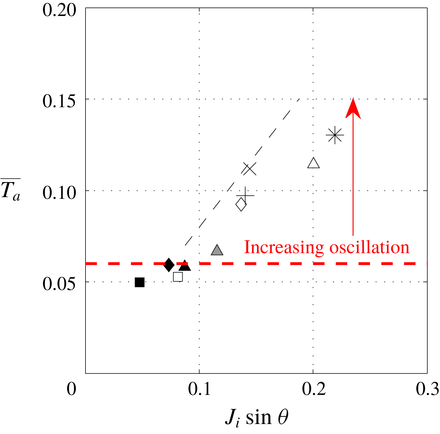
Overall acceleration parameter
 $\overline{T_{a}}=(\unicode[STIX]{x1D6FF}_{i}/U_{i})((U_{c}-U_{i})/x_{c})$
as a function of
 $J_{i}\sin \unicode[STIX]{x1D703}$
. The black dashed line indicates the theoretical relation
 $\overline{T_{a}}\approx 0.8J_{i}\sin \unicode[STIX]{x1D703}$
. The horizontal red dashed line indicates
 $\overline{T_{a}}=0.06$
.

Negretti et al. (Reference Negretti, Flòr and Hopfinger2017) explained the current development on slopes by introducing an overall acceleration parameter
 $\overline{T_{a}}=(h_{i}/x_{c})(\unicode[STIX]{x0394}U/U_{m})$
, with the velocity difference
 $\unicode[STIX]{x0394}U$
from the beginning of the slope to
 $x_{c}$
. They suggested that when
 $\overline{T_{a}}>0.05$
velocity oscillations exist whereas when
 $\overline{T_{a}}<0.05$
the velocity increase is regular, approaching an equilibrium state within approximately
 $10h_{0}$
. In the more general case, where the initial conditions are varied (which was not the case in Negretti et al.
Reference Negretti, Flòr and Hopfinger2017), a physically more appropriate definition of an overall acceleration parameter is
 $$\begin{eqnarray}\overline{T_{a}}=\frac{\unicode[STIX]{x1D6FF}_{i}}{U_{i}}\frac{U_{c}-U_{i}}{x_{c}}.\end{eqnarray}$$
This acceleration parameter can be expressed in terms of the initial Richardson number and slope angle by relating
 $U_{c}$
to the critical Richardson number
 $J_{c}$
and getting
 $x_{c}$
from assuming free fall up to
 $x_{c}$
. This gives
 $$\begin{eqnarray}\overline{T_{a}}\approx J_{i}\sin \unicode[STIX]{x1D703}\frac{2C}{\left(1+\left({\displaystyle \frac{\unicode[STIX]{x1D6FF}_{i}}{J_{c}h_{i}}}\right)^{1/3}\right)},\end{eqnarray}$$
where
 $C$
is a function of the ratio of
 $u_{m}/U$
and of
 $(u_{m}-u_{min})/U$
. In experiments D1 and D2,
 $C\approx 1.1$
and in D0, with larger back flow,
 $C\approx 1.3$
, giving respectively
 $\overline{T_{a}}\approx 0.8J_{i}\sin \unicode[STIX]{x1D703}$
and
 ${\approx}1.1J_{i}\sin \unicode[STIX]{x1D703}$
. A similar dimensionless number is defined in Negretti, Socolofsky & Jirka (Reference Negretti, Socolofsky and Jirka2008), using a temporal linear stability, normal modes, analysis of a two-layer stratified exchange flow. There it is shown that the growth rate of the instability depends on the acceleration parameter. Figure 7 shows
 $\overline{T_{a}}$
as a function of
 $J_{i}\sin \unicode[STIX]{x1D703}$
for all the performed experiments, including those of Negretti et al. (Reference Negretti, Flòr and Hopfinger2017) and Pawlak & Armi (Reference Pawlak and Armi2000). The pre-factor
 $0.8$
shown in the figure by the dashed line compares reasonably well with the experimental value determined from (5.1). Although the definition of
 $\overline{T_{a}}$
differs from that of Negretti et al. (Reference Negretti, Flòr and Hopfinger2017), we see that transition from no velocity oscillations to oscillations of increasing amplitude with increasing
 $\overline{T_{a}}$
is at
 $\overline{T_{a}}\approx 0.06$
. In experiment D2-15 for instance, with
 $\overline{T_{a}}\approx 0.12$
velocity oscillations are large. When
 $\overline{T_{a}}\leqslant 0.05$
, D0, the increase in velocity up to an equilibrium state is smooth.
6 Entrainment and bottom drag
6.1 Determination of the entrainment coefficient
The entrainment rate is defined as the volume of ambient fluid engulfed into the current along its descent. It can obtained from the discretization of (4.1b
), i.e. taking the difference between the input and the output fluxes in a control volume with a longitudinal width
 $\unicode[STIX]{x0394}x$
, here taken equal to
 $h_{i}$
. The entrainment coefficient is thus
 $$\begin{eqnarray}E_{q}=\frac{1}{U(x)}\frac{q(x+h_{i}/2)-q(x-h_{i}/2)}{h_{i}}.\end{eqnarray}$$
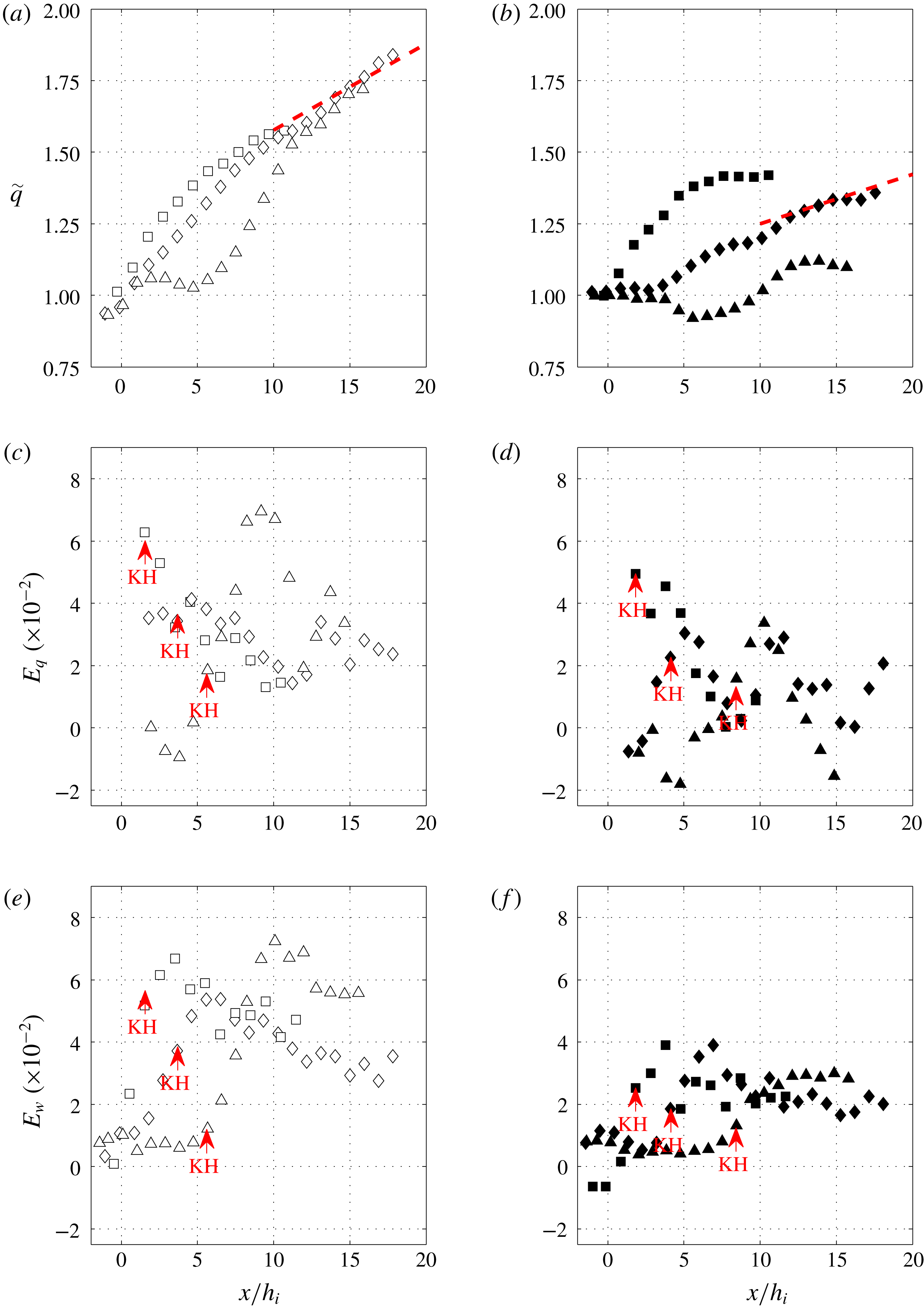
Figure 8(a,b) shows the variation in volume flux as a function of
 $x/h_{i}$
. As is evident from the data, a direct calculation of the gradient would give large variations. A primary source of error in these estimates of the volume flux gradient results from the slow variation at the origin of the instabilities. In order to reduce the variations, the gradient is determined using a moving averaging filter of spatial width
 $L={\mathcal{L}}$
and sub-sampling the data with the same spatial scale. The dashed lines in figure 8(a,b) at
 $x/h_{i}>10$
indicate the expected entrainment rate of an equilibrium current. It is seen that in figure 8(a) there is good agreement whereas in the experiments with a slope of
 $7^{\circ }$
in figure 8(b) there is a relatively large variation because values are very small.
The entrainment coefficients obtained using (6.1) are shown in figure 8(c,d). In experiments D0 (▫) the highest entrainment coefficient is near the beginning of the slope, corresponding to the beginning of KHI, it then decreases along the slope down to a value of approximately 0.02 on slope
 $15^{\circ }$
, whereas in the experiments on slope of
 $7^{\circ }$
,
 $E_{q}$
decreases to approximately 0.005. This is in agreement with the behaviour observed by Pawlak & Armi (Reference Pawlak and Armi2000). While in experiments D2 and D1, the final values are similar, the highest values are observed shortly after KHI. These highest values of entrainment rates are close to
 $0.065\pm 0.005$
for larger slope angles and
 $0.04\pm 0.1$
for the smallest slope angles, which are values similar to what is observed in free shear layers.
Time-averaged flow rate
 $q/q_{i}$
of the gravity current as a function of
 $x/h_{i}$
(a,b). The dashed line at
 $x/h_{i}>10$
corresponds to Ellison & Turner’s (Reference Ellison and Turner1959) equilibrium entrainment. Time-average entrainment coefficient
 $E_{q}$
(c,d) and
 $E_{w}$
(e,f) as a function of
 $x/h_{i}$
. (a,c,e)
 $15^{\circ }$
(empty symbols) and (b,d,f)
 $7^{\circ }$
(filled symbols). D0 (▫, ▪), D1 (♢, ♦) and D2 (▵, ▴).

Another estimate of entrainment is obtained from the velocity
 $w_{h}$
normal to the interface as proposed by Morton & Turner (Reference Morton and Turner1956). The
 $z$
-integrated continuity equation gives
 $$\begin{eqnarray}E_{w}=-\frac{w_{h}}{U}.\end{eqnarray}$$
To minimize errors, we estimated the velocity
 $w_{h}$
at the interface from the PIV velocity data by averaging three values of the normal velocity around the averaged value of
 $h$
for each
 $x$
-position and normalizing with the depth integrated velocity at the same location. We also compared the values obtained directly from averaged velocity fields and interface positions and from instantaneous velocity fields and interface positions averaged after. The differences between the two methods is small. Details on the experimental errors relative to the entrainment are given in appendix A.
The entrainment rates
 $E_{w}$
are shown in figure 8(e,f) for the experiments with slope of
 $15^{\circ }$
and
 $7^{\circ }$
, respectively. As already reported by Odier et al. (Reference Odier, Chen and Ecke2014), there are large differences in
 $E_{q}$
and
 $E_{w}$
. In general, the entrainment
 $E_{w}$
is larger than
 $E_{q}$
and after the first acceleration region and establishment of the shear layer, the two differ by a factor of two at
 $x/h_{i}>10$
:
 $E_{w}\approx 0.05$
and
 $E_{q}\approx 0.02$
for the larger slopes and
 $E_{w}\approx 0.02$
and
 $E_{q}\approx 0.01$
for
 $\unicode[STIX]{x1D703}=7^{\circ }$
. These values are similar to those obtained by Odier et al. (Reference Odier, Chen and Ecke2014) (cf. their figure 13):
 $E_{q}\approx 0.02$
and
 $E_{w}\approx 0.04$
.
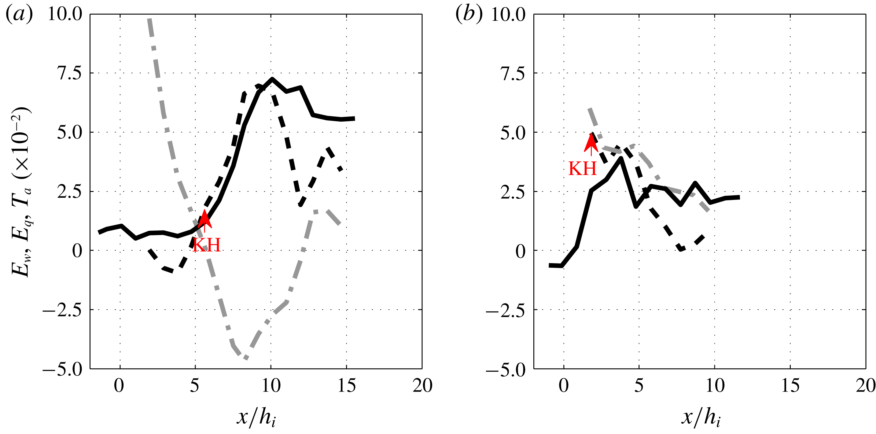
Entrainment coefficient
 $E_{w}=-w_{h}/U$
(continuous lines),
 $E_{q}=(\text{d}q/\text{d}x)/U$
(dashed-line) and
 $T_{a}=(h/U)\,\text{d}U/\text{d}x$
(dash-dotted line) of experiments D2-15 (a) and D0-7 (b).

In figure 9 these differences are highlighted by plotting
 $E_{q}$
(dashed lines),
 $E_{w}$
(continuous lines) and
 $T_{a}=(h/U)\,\text{d}U/\text{d}x$
(grey dash-dotted lines) for experiments D2-15 (a) and D0-7 (b). After the acceleration region, in which entrainment is small or nearly inexistent in the absence of interfacial instabilities, in the D2-15 experiment both
 $E_{q}$
and
 $E_{w}$
increase and reach a maximum value of
 ${\approx}0.07$
and then
 $E_{q}$
decreases rapidly down to 0.02, while
 $E_{w}\approx 0.05$
. In the experiment D0-7, we observe a discrepancy at the beginning, with
 $E_{q}>E_{w}$
until the beginning of KHI, while the discrepancy between the two definitions is smaller further downstream in this case. The grey dash-dotted lines in both figures represent the acceleration parameter
 $T_{a}=(h/U)\text{d}U/\text{d}x$
, which can be seen as part of the entrainment,
 $E_{q}=T_{a}+\text{d}h/\text{d}x$
, as outlined in Negretti et al. (Reference Negretti, Flòr and Hopfinger2017). In experiment D2-15 (figure 9
a),
 $T_{a}$
is large at the beginning, is negative after the beginning of KHI to become weakly positive at
 $x/h_{i}\approx 12$
. For experiment D0-7 (figure 9
b) we see that for
 $0<x/h_{i}<4$
,
 $T_{a}\approx E_{q}$
, so that the current depth is nearly constant, and then decreases toward zero. Since at slope angles
 $\unicode[STIX]{x1D703}\leqslant 15$
equilibrium entrainment rates are very small, errors in measuring entrainment rates can be large, particularly in
 $E_{q}$
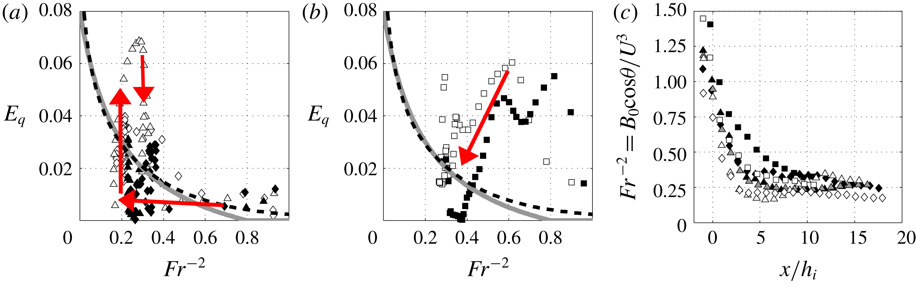
. Nevertheless, entrainment coefficients determined from the change in volume flux
 $E_{q}$
tend toward the values known for equilibrium flow conditions as seen in figure 10 by comparing (a) and (b) for experiments D2 and D0, respectively. Red arrows highlight the path toward the equilibrium values for the two release cases: it is direct in the D0 experiments with a smooth increase, while for the D2 experiments there is also an oscillation in the Richardson number before reaching a constant equilibrium value in figure 4(a). This behaviour is consistent with the variation with downstream distance of the Froude number
 $Fr$
(figure 10
c), which also tends toward the equilibrium values expected for the slopes considered. The expected equilibrium is represented in figure 10(a,b) by the empirical relations proposed by Turner (Reference Turner1986) and Cenedese & Adduce (Reference Cenedese and Adduce2010) deduced from gravity currents at equilibrium;
 $E_{w}$
, in contrast, overestimates the values known for equilibrium flow conditions. Odier et al. (Reference Odier, Chen and Ecke2014) suggest taking an average between
 $E_{w}$
and
 $E_{q}$
for the equilibrium entrainment value, which is hardly satisfying.
Krug et al. (Reference Krug, Holzner, Lüthi, Wolf, Kinzelbach and Tsinober2013) also find
 $E_{w}=0.04$
for their gravity current on a slope of
 $10^{\circ }$
, and suggest that this is the correct entrainment coefficient at equilibrium state of the current. The difference with respect to Ellison & Turner (Reference Ellison and Turner1959) is attributed to larger Reynolds numbers in their experiments. Visibly, this is not the case. In the present experiments we also obtain
 $E_{w}\approx 0.04$
, but
 $E_{q}\approx 0.02$
when the equilibrium state is approached, in agreement with Pawlak & Armi (Reference Pawlak and Armi2000), van Reeuwijk, Holzner & Caulfield (Reference van Reeuwijk, Holzner and Caulfield2019), Odier et al. (Reference Odier, Chen and Ecke2014) and even Krug et al. (Reference Krug, Holzner, Lüthi, Wolf, Kinzelbach and Tsinober2013). Indeed, from their figure 12, we obtain
 $E_{q}=\text{d}h/\text{d}x$
close to 0.02 in the equilibrium state at a distance ten times the inlet height, i.e. at
 $x>52~\text{cm}$
. In the present experiments
 $E_{w}\approx E_{q}$
at the beginning of KH instability when the mixing length
 $\ell _{m}$
is expected to be large (large scale overturning), but when the equilibrium state is approached the mixing length decreases and
 $E_{q}<E_{w}$
. Krug et al. (Reference Krug, Holzner, Lüthi, Wolf, Kinzelbach and Tsinober2013) present measurements of
 $W$
over a large range of
 $z$
and it is seen that
 $W/U=0.04$
at the interface and drops to zero at
 $\unicode[STIX]{x0394}z\approx 0.3h$
away from it. This is indicative of a small mixing length; in Krug et al. (Reference Krug, Holzner, Lüthi, Wolf, Kinzelbach and Tsinober2013)
 $\ell _{m}\approx h/10$
. For the foregoing reasons we take
 $E_{q}$
as the physically correct entrainment coefficient.
Entrainment rates
 $E_{q}$
as a function of
 $Fr^{-2}$
for experiments D2 (a) and D0 (b). Relation proposed by Turner (Reference Turner1986) (black dashed line) and Cenedese & Adduce (Reference Cenedese and Adduce2010) (grey continuous line). The red arrows indicate the path toward a constant equilibrium value down the slope (for the D2 experiments for instance,
 $Fr^{-2}$
first decreases, reaches a minimum then increases again and stabilizes on a constant value). (c) Inverse of the squared Froude number
 $Fr^{-2}=B_{0}\cos \unicode[STIX]{x1D703}/U^{3}$
as a function of
 $x/h_{i}$
,
 $7^{\circ }$
(filled symbols),
 $10^{\circ }$
(grey symbols) and
 $15^{\circ }$
(empty symbols); D0 (▫, ▪), D1 (♢, ♦) and D2 (▵, ▴ (grey), ▴).

6.2 Bottom drag coefficient
In viscous flows,
 $c_{D}$
is inversely proportional to the Reynolds number, as has been shown by Cenedese et al. (Reference Cenedese, Whitehead, Ascarelli and Ohiwa2004) for a gravity current of
 $Re<300$
. In the present experiments
 $Re>1400$
(for D2-15,
 $Re=Uh/\unicode[STIX]{x1D708}\approx 1700$
at the beginning of the slope and is
 $Re\approx 2800$
at
 $x/h_{i}=15$
). Hence, the boundary layer region is turbulent after onset of KH instability. In this case we use known values and expressions for a turbulent boundary region. For a wall jet (that has a velocity profile similar to a gravity current) of Reynolds number
 $Re_{m}=u_{m}z_{m}/\unicode[STIX]{x1D708}\approx 10^{3}$
, where
 $z_{m}$
is the height of maximal velocity,
 $u_{m}\approx 8~\text{cm}~\text{s}^{-1}$
the maximal velocity and
 $\unicode[STIX]{x1D708}\approx 10^{-2}~\text{cm}^{2}~\text{s}^{-1}$
the viscosity,
 $c_{D}\approx 5\times 10^{-3}$
(George et al.
Reference George, Abrahamsson, Eriksson, Karlsson, Löfdahl and Wosnik2000). For a turbulent boundary layer
 $c_{D}$
is given by the empirical relation
 $c_{D}=0.0113{Re_{m}}^{-0.178}$
, which gives a value close to the bottom drag coefficient for a wall jet at the same Reynolds number. These bottom drag coefficients are small compared with the large values determined for gravity currents on slopes in the present experiments (see figure 11 and also 12) and those of Negretti et al. (Reference Negretti, Flòr and Hopfinger2017). This is due to the interaction of KH billows with the boundary region and not due to boundary layer turbulence. Therefore, the known Reynolds number dependency of the boundary layer drag coefficient does likely not apply for gravity currents on slopes, whereas for gravity currents on horizontal boundaries, the classical boundary layer values apply with the drag coefficient tending asymptotically towards
 $10^{-3}$
, when Reynolds numbers are very large (Cossu & Wells Reference Cossu and Wells2012).
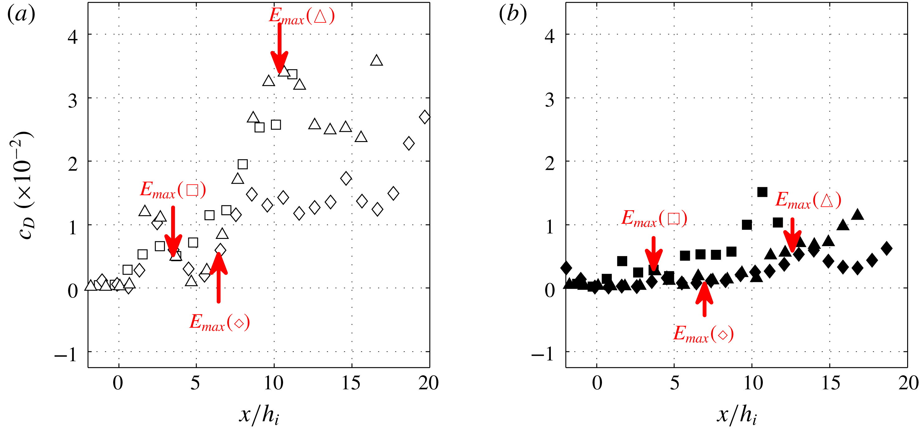
Experimental bottom drag coefficient
 $c_{D}$
from (6.3) as a function of
 $x/h_{i}$
for (a)
 $15^{\circ }$
(empty symbols) and (b)
 $7^{\circ }$
(filled symbols). The arrows indicate the location of maximum entrainment. D0 (▫, ▪), D1 (♢, ♦) and D2 (▵, ▴).

Since accurate velocity measurements are difficult close to the bottom boundary, we estimated
 $c_{D}$
using an average of the Reynolds stresses
 $\overline{u^{\prime }w^{\prime }}$
and the local averaged velocity
 $$\begin{eqnarray}c_{D}=\frac{1}{\unicode[STIX]{x1D6FF}_{B}}\int _{z(u=0)}^{z(u=u_{m})}\frac{\overline{u^{\prime }w^{\prime }}}{U^{2}}\,\text{d}z,\end{eqnarray}$$
where
 $\unicode[STIX]{x1D6FF}_{B}$
is the distance from the bottom boundary where the local velocity becomes maximum. Figure 11 shows the variation of
 $c_{D}$
with downstream distance
 $x/h_{i}$
on slope
 $15^{\circ }$
(a) and slope
 $7^{\circ }$
(b). We see that in the first region on the slope the values of
 $c_{D}$
are very small in all conducted experiments,
 $O(10^{-3})$
. In D0 and D1 experiments, where
 $\unicode[STIX]{x1D6FF}/h<1$
, there is a shift between the location of maximum entrainment and maximum
 $c_{D}$
, while in D2 experiments where
 $\unicode[STIX]{x1D6FF}/h\approx 1$
these locations coincide. This is also evident from figure 2(c,f,i), where the Reynolds stress
 $\overline{u^{\prime }w^{\prime }}/u_{m}^{2}$
reaches a maximum both in the boundary layer and at the interface, with opposite signs, in the D2 experiment (c), while there is a shift between the maximum Reynolds stress in the shear layer and at the bottom boundary for the experiments D1 (f) and D0 (i). From figure 11 the maximum values reached by
 $c_{D}$
are of
 $O(10^{-2})$
, and thus very large, as already reported by Negretti et al. (Reference Negretti, Flòr and Hopfinger2017). The values are respectively
 $c_{D}\approx 0.03$
and
 $0.015$
for the
 $15^{\circ }$
slope and
 $7^{\circ }$
slope.
In order to highlight the relation between current acceleration, entrainment and bottom drag, we display in figure 12 the variation with downstream distance of the three quantities for experiments on slope
 $\unicode[STIX]{x1D703}=15^{\circ }$
. Figure 12(a) suggests that the strongest decrease in velocity after its maximum value takes place when the maxima of entrainment and bottom friction are correlated (D2 experiment). In the D2 experiment the current accelerates when both entrainment and bottom drag are small. At maximum velocity, entrainment and drag start to increase rapidly and the current velocity starts to decrease to then increase again after maximum values of
 $E_{w}$
and
 $c_{D}$
. This figure also shows the correlation between entrainment and bottom drag. In D1 and D0 experiments (figure 12
b), the rate of velocity increase changes when
 $E_{w}$
reaches a maximum and
 $c_{D}$
starts to increase. Here, there is a shift between maximum entrainment and maximum bottom drag and this is larger in the D0 experiment (figure 12
c).
In D2 experiments, the bottom drag
 $c_{D}$
increases when the entrainment coefficient
 $E_{q}$
increases. The link between the upper and the lower part of the gravity current in the D2 configuration is evident in figure 2: we observe that the normalized Reynolds stress
 $\overline{u^{\prime }w^{\prime }}/U^{2}$
, at the interface and at the bottom, increases at the same location (with opposite signs). The spatial correlation coefficient that we estimated between these two terms is above
 $0.75$
for the D2 configuration and below
 $0.25$
for the D0 configuration.
Dallimore et al. (Reference Dallimore, Imberger and Ishikawa2001) use the turbulent kinetic energy budget of Sherman, Imberger & Corcos (Reference Sherman, Imberger and Corcos1978) for a uniform flow to link entrainment to the bottom drag. This correlation does not apply in the present strongly developing flow. In general
 $c_{D}=f(E_{q},\unicode[STIX]{x1D6FF}/h,Fr,\unicode[STIX]{x1D70F}_{\unicode[STIX]{x1D708}})$
, where
 $\unicode[STIX]{x1D70F}_{\unicode[STIX]{x1D708}}$
is the viscous shear stress. Since
 $E_{q}$
depends on
 $Fr$
and
 $\unicode[STIX]{x1D70F}_{\unicode[STIX]{x1D708}}$
is negligible, the important parameters are
 $E_{q}$
and the wall proximity, expressed by
 $\unicode[STIX]{x1D6FF}/h$
, which introduces a shift in
 $c_{D}$
with respect to
 $E_{q}$
when
 $\unicode[STIX]{x1D6FF}/h<1$
at instability onset. Maximum
 $c_{D}$
occurs when the interfacial layer approaches the wall, i.e. when
 $\unicode[STIX]{x1D6FF}/h\geqslant 1$
. The D2 experiments (figure 12
d) indicate a linear relation between
 $E_{q}$
and
 $c_{D}$
of the form
 $$\begin{eqnarray}c_{D}\approx B(E_{q}-E_{i}),\end{eqnarray}$$
with
 $B\approx 0.6$
and the initial value
 $E_{i}\approx 0.01$
. In figure 12(d) the bottom drag coefficient
 $c_{D}$
is plotted as a function of
 $E_{q}$
and compared with the empirical expression (6.4).
Time-averaged depth integrated velocity
 $U/U_{i}$
(black continuous line), entrainment coefficient
 $E_{w}$
(blue dash-dotted line),
 $E_{q}$
(blue dotted line) and bottom drag coefficient
 $c_{D}$
(blue dashed line) versus
 $x/h_{i}$
. (a) D2-15, (b) D1-15 and (c) D0-15. (d) Bottom drag coefficient
 $c_{D}$
as a function of the entrainment
 $E_{q}$
for slopes
 $7^{\circ }$
and
 $15^{\circ }$
(filled and open symbols). D0 (▫, ▪), D1 (♢, ♦), D2 (▵, ▴). The dashed line indicates the empirical relation
 $c_{D}\approx B(E-E_{i})$
with
 $B\approx 0.6$
and
 $E_{i}\approx 0.01$
.

The experimental entrainment coefficients and bottom drag are used in the following section to solve numerically the integrated equation (7.1).
7 Comparison with numerical solutions of the governing equations
Equation (4.4) has been solved numerically to obtain the three unknown variables
 $U$
,
 $h$
,
 $\overline{g^{\prime }}$
using a Runge–Kutta scheme of order 4 (RK4) with a step
 $\text{d}x=10^{-2}~\text{mm}$
, using the experimental entrainment
 $E=E_{q}(x)$
and bottom friction
 $c_{D}(x)$
. The shape factors were obtained from the 2.5 layer model derived in appendix B, and are
 $S_{1}=0.5$
and
 $S_{2}=0.6$
. Neglecting the spatial variations of
 $S_{1}$
,
 $S_{2}$
and
 $S_{3}$
, the numerical solution has been obtained solving the following equation:
 $$\begin{eqnarray}\frac{\text{d}\tilde{U} }{\text{d}\tilde{x}}=\frac{S_{2}\tilde{U} ^{2}\sin \unicode[STIX]{x1D703}-\tilde{U} ^{5}(c_{D}+E)-S_{1}E\cos \unicode[STIX]{x1D703}\tilde{U} /2-(\tilde{q}/\tilde{R})(S_{3}E\tilde{U} ^{4}+S_{1}\sin \unicode[STIX]{x1D703}\tilde{U} /2)}{\tilde{q}(U^{3}-S_{1}\cos \unicode[STIX]{x1D703})}.\end{eqnarray}$$
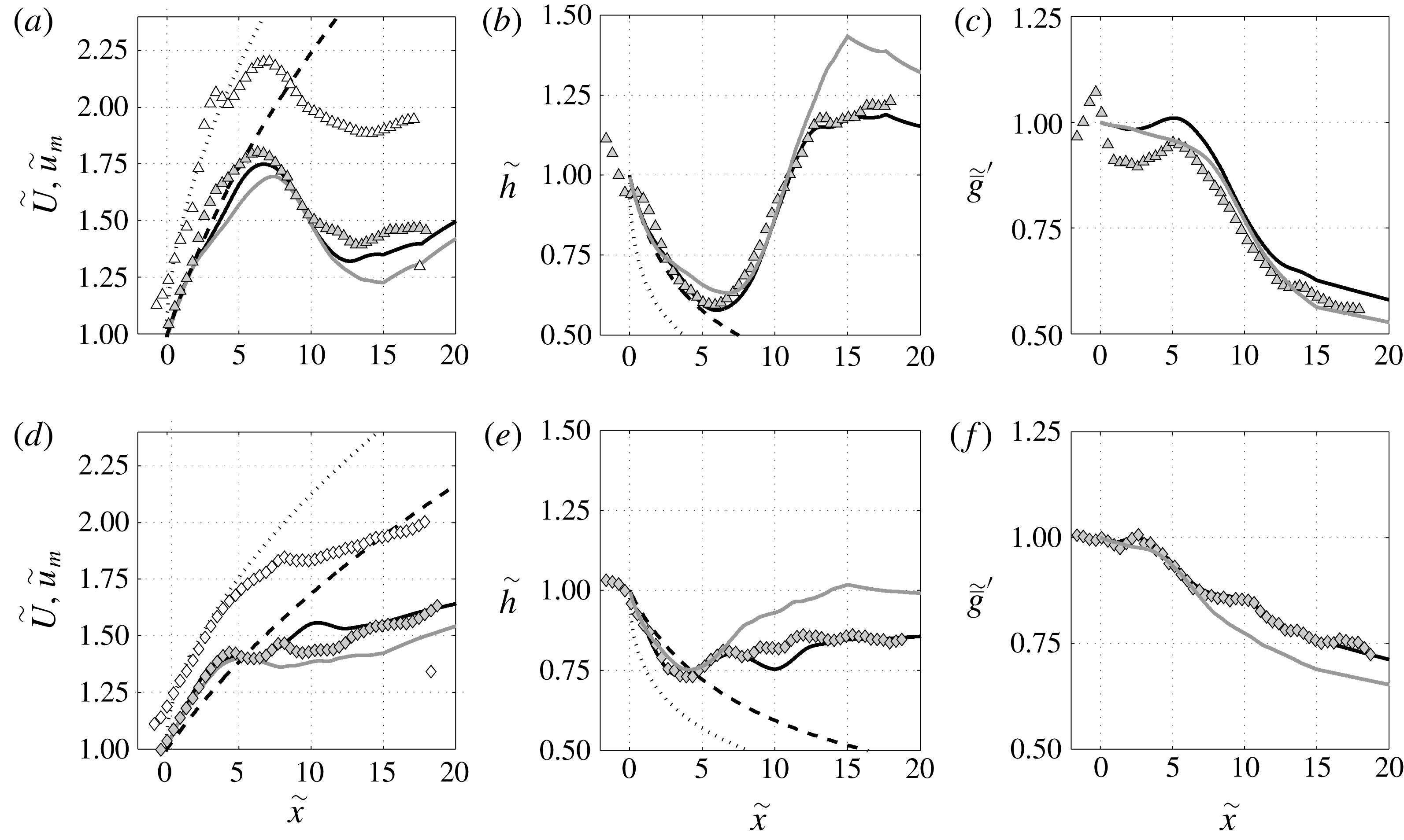
Figure 13 presents the comparison between the experimental data (symbols) of the depth integrated
 $\tilde{U}$
and maximum
 $\tilde{u} _{m}$
velocities (a,d), the current depth
 $\tilde{h}$
(b,e) and the depth integrated buoyant acceleration
 $\tilde{\overline{g}}^{\prime }$
(c,f) to various solutions for two contrasted experiments D2-15 (a–c) and D1-7 (d–f). The experimental values of
 $\tilde{\overline{g}}^{\prime }$
in figure 13(c,f) have been calculated indirectly as
 $\tilde{\overline{g}}^{\prime }=B_{0}/(Uh)$
since the downstream spatial variation of the density fields could not be extrapolated from the fluorescent dye visualizations. The numerical solution of (7.1) is represented by continuous lines, black lines using
 $E_{q}$
and grey lines using
 $E_{w}$
. The free fall solution proposed in Negretti et al. (Reference Negretti, Flòr and Hopfinger2017) is represented by dashed lines and the implicit shallow water (SW) solution (4.6) with
 $S_{1}=S_{2}=1$
by dotted lines. We tested the numerical solution for all experiments and found a very good agreement, the best agreement for all variables
 $\tilde{U}$
,
 $h$
and
 $\tilde{\overline{g}}^{\prime }$
using the numerical solution of (7.1),
 $E_{q}$
and
 $c_{D}$
from figure 11, over the full measured domain.
Comparison of the theoretical models and numerical solutions (lines) and the experimental data (symbols) for D2-15 (a–c) and D1-17 (d–f). RK4 Numerical solution (continuous line) for
 $E_{w}$
(grey line) and
 $E_{q}$
(black line) and for
 $S_{1}$
and
 $S_{2}$
obtained from the 2.5 layer model (appendix B). Implicit shallow water solution (dotted line), free fall velocity with
 $S_{2}=0.75$
(dashed line). (a,d)
 $\tilde{U}$
(grey symbols) and
 $\tilde{u} _{m}$
(white symbols); (b,e)
 $\tilde{h}$
and (c,f)
 $\tilde{\overline{g}}^{\prime }$
.

The SW solution (4.6) reproduces fairly well the data for
 $\tilde{u} _{m}$
and badly those relative to
 $h$
in the first accelerating region, in which entrainment and bottom friction can be neglected. It is curious to see how the free fall relation proposed by Negretti et al. (Reference Negretti, Flòr and Hopfinger2017) reproduces well the data for
 $\tilde{U}$
in the same region, neglecting the pressure term with respect to the SW model: the positive contribution given by the pressure term is compensated by the shape factor
 $S_{1}$
. Also, the critical distance
 $x_{c}$
is well detected for both the velocity and the current depth. We tested solving (7.1) initialized using the constant entrainment coefficient of Turner (Reference Turner1973) (not shown) and constant
 $c_{D}=10^{-3}$
and observed a bad agreement with the experimental data. Sensitivity tests with different shape factors show that the numerical solution for
 $\tilde{U}$
,
 $h$
and
 $\tilde{\overline{g}}^{\prime }$
strongly depends on these parameters, which justifies the importance in their proper estimation as we made in appendix B.
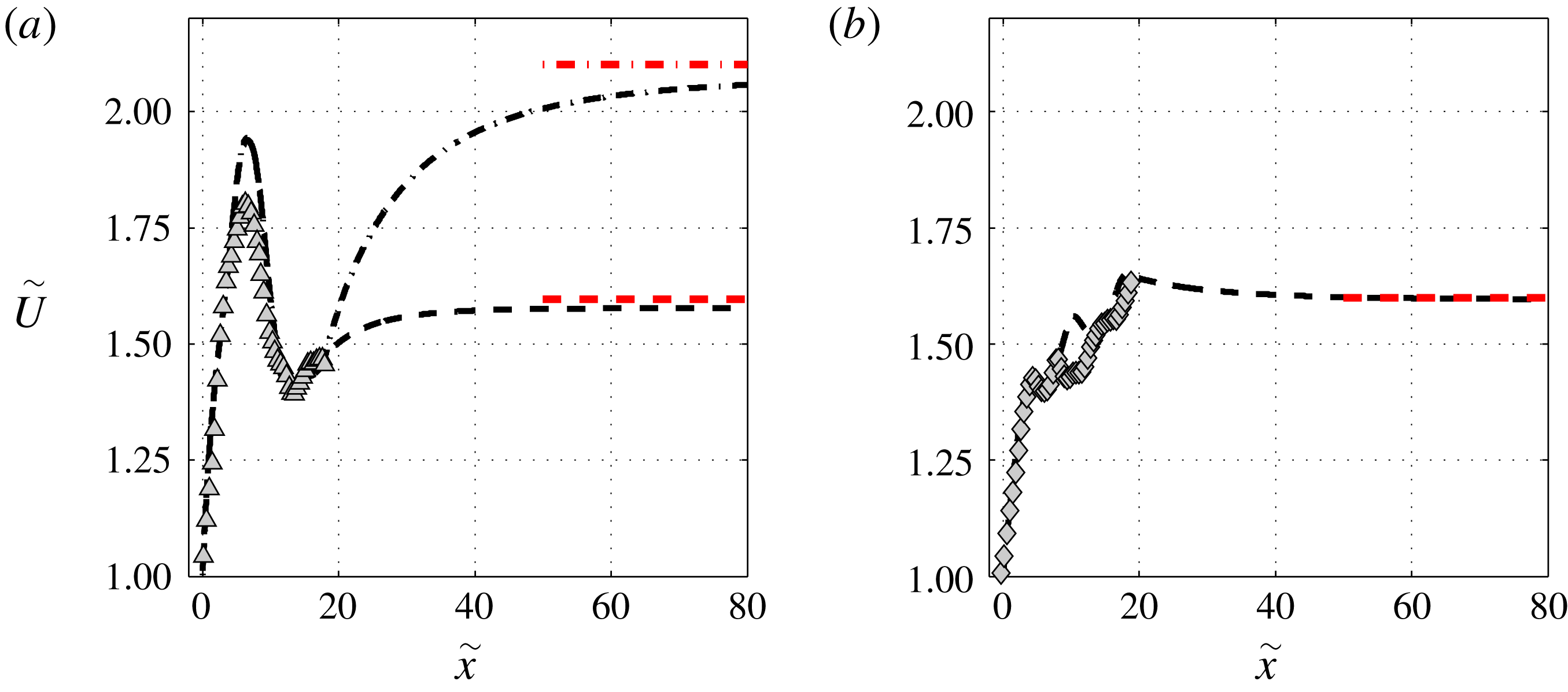
Predictions of the equilibrium state velocity
 $\tilde{U} _{n}$
using (4.6) and (7.2) with
 $\{S_{1},S_{2}\}=\{0.67,0.75\}$
for (a) D2-15 (▵) and (b) D2-7 (♢). For
 $\tilde{x}<18$
the experimental entrainment
 $E_{q}$
and bottom drag
 $c_{D}$
have been used to solve the numerical model. For
 $\tilde{x}>18$
,
 $E=2\times 10^{-2}$
,
 $c_{D}=3\times 10^{-3}$
(
 $-\cdot$
) and
 $c_{D}=3\times 10^{-2}$
(
 $--$
) (a) and
 $E=1.5\times 10^{-2}$
,
 $c_{D}=5\times 10^{-3}$
(b) from the equilibrium values. The horizontal red dashed and dash-dotted lines are the equilibrium velocities from (7.2).

We can use the numerical solution to predict the distance needed to reach the equilibrium between the gravity and the drag terms
 $x_{n}$
where acceleration ceases and the flow attains a constant velocity. The dimensionless equilibrium velocity
 $\tilde{U} _{n}$
defined in Negretti et al. (Reference Negretti, Flòr and Hopfinger2017) from their (2.11) and here obtained from (4.4) is
 $$\begin{eqnarray}\tilde{U} _{n}=\left(\frac{S_{2}\sin \unicode[STIX]{x1D703}}{c_{D}+E\left(1+\frac{1}{2}S_{1}Ri\right)}\right)^{1/3}=\left(\frac{S_{2}\sin \unicode[STIX]{x1D703}-{\displaystyle \frac{1}{2}}S_{1}E\cos \unicode[STIX]{x1D703}}{c_{D}+E}\right)^{1/3},\end{eqnarray}$$
where
 $Ri=B_{0}\cos \unicode[STIX]{x1D703}/U^{3}$
. The right-hand side term of (7.2) is deduced from the differential equation for
 $Ri$
in Ellison & Turner (Reference Ellison and Turner1959) (their equation (13)) by assuming
 $\text{d}Ri/\text{d}x=0$
.
In figure 14 the solutions of (7.1) are shown for experiments D2-15 (a) and D1-7 (b). The equilibrium values, given by (7.1) are indicated by the horizontal red lines, for experiment D2-15:
 $Ri=0.25$
,
 $E=0.02$
and
 $c_{D}=3\times 10^{-3}$
(higher value of
 $\tilde{U} _{n}$
, dash-dotted line) and
 $c_{D}=3\times 10^{-2}$
(lower value of
 $\tilde{U} _{n}$
, dashed line), as extrapolated from figures 8 and 11. It is interesting to point out that the two relations proposed by Ellison & Turner (Reference Ellison and Turner1959) for
 $E(\unicode[STIX]{x1D703})$
and
 $E(Ri)$
coincide only if assuming a large
 $c_{D}$
: the dashed line in figure 14(a) is equivalent using
 $E(\unicode[STIX]{x1D703})$
and
 $E(Ri)$
only if a large value of
 $c_{D}=3\times 10^{-2}$
is used. Figure 14(b) shows the velocity variation for D2-7, taking in this case
 $E=0.015$
and
 $c_{D}=0.005$
(cf. figures 8 and 11).
Figure 14 indicates that the gravity current needs a distance of
 $40\tilde{x}$
to reach an equilibrium state, which is much larger than the commonly assumed distance of
 $10\tilde{x}$
. No extrapolation is needed for the D0 experiment because, as seen in figure 12(c),
 $\tilde{U}$
has practically reached its equilibrium value at
 $\tilde{x}\approx 10$
.
8 Further discussion and conclusions
The four important conclusions that emerge are: (i) the development of gravity currents on slopes can be regular or highly irregular depending on the interfacial instability conditions at the beginning of the slope and on slope angle and this is expressed by an overall acceleration parameter; (ii) the bottom drag coefficient is large and cannot be neglected even in an equilibrium current and, more importantly, it is related to the interfacial entrainment rate; (iii) the entrainment coefficients determined from the change in volume flux
 $E_{q}=(\text{d}q/\text{d}x)/U$
on the one hand and from velocity measurements at the outer interface of the current
 $E_{w}=-w_{h}/U$
on the other, are different when flow equilibrium is approached, as already observed by Odier et al. (Reference Odier, Chen and Ecke2014). While Odier et al. (Reference Odier, Chen and Ecke2014) suggest taking an average between
 $E_{w}$
and
 $E_{q}$
for the equilibrium entrainment value, we give arguments, based on turbulent shear stress measurements, that the equilibrium value is
 $E_{q}$
, in accordance with Pawlak & Armi (Reference Pawlak and Armi2000); (iv), when the initial interfacial Richardson number and slope angles are such that
 $\overline{T_{a}}$
is large, an equilibrium state is reached at a distance of approximately
 $50h_{0}$
(instead the usually assumed distance of
 $10h_{0}$
).
The current development is shown to depend on slope angle and on the interfacial Richardson number at the beginning of the slope
 $J_{i}=\unicode[STIX]{x1D6FF}_{i}{g_{0}}^{\prime }/\unicode[STIX]{x0394}u_{i}^{2}$
, where
 $\unicode[STIX]{x1D6FF}_{i}$
,
 $\unicode[STIX]{x0394}u_{i}$
and
 ${g_{0}}^{\prime }$
are, respectively, the velocity interface thickness, the maximum velocity difference and reduced gravity at slope origin. When
 $J_{i}$
is small, here
 $J_{i}<0.3$
, as is the case in outflow over a sill (Pawlak & Armi Reference Pawlak and Armi2000) or inflow at the beginning of the slope (here D0 experiment), an equilibrium flow of constant velocity is reached at the expected downstream distance of approximately
 $10h_{i}$
, where
 $h_{i}$
is the current height at the beginning of the slope estimated with (4.2.a,b
). For this reason, the development phase is often neglected as in Dallimore et al. (Reference Dallimore, Imberger and Ishikawa2001) or Odier et al. (Reference Odier, Chen and Ecke2014). However, as has already been demonstrated by Negretti et al. (Reference Negretti, Flòr and Hopfinger2017), the flow development can be entirely different, approaching equilibrium much further downstream, when the initial interfacial Richardson number and slope angle are large. The flow development is shown to depend on an overall acceleration parameter
 $\overline{T_{a}}=(\unicode[STIX]{x1D6FF}_{i}/U_{i})(U_{c}-U_{i}/x_{c})$
, which, to first order, is given by
 $J_{i}\sin \unicode[STIX]{x1D703}$
, where
 $U_{i}$
is the velocity at the beginning of the slope and
 $U_{c}$
and
 $x_{c}$
are, respectively, the velocity and position at instability onset. When
 $\overline{T_{a}}<0.06$
the velocity increases steadily toward an equilibrium state, whereas at large values of
 $\overline{T_{a}}$
the development is highly irregular with large velocity variation.
To summarize the current development, there are three different regimes depending on the overall acceleration parameter. When
 $\overline{T_{a}}$
is large,
 $\overline{T_{a}}\approx 0.12$
, as in the D2-15 experiments, the current strongly accelerates up to
 $x=x_{c}$
, reaching a maximum of velocity at the beginning of KHI, then decelerates and finally re-accelerates again. In this case the velocity oscillations are large, due to the large scale, intense vortical structures at the start of KHI that cause sudden large entrainment and boundary layer separation because
 $(\unicode[STIX]{x1D6FF}/h)_{c}\geqslant 1$
, and thus spatially correlated high values of the bottom drag coefficient (see § 6). In the second regime,
 $0.06<\overline{T_{a}}<0.1$
, corresponding to the D1 experiments, the current undergoes an abrupt change in acceleration at
 $x=x_{c}$
. In this case, the interface is thinner,
 $0.3<J_{i}<0.6$
and
 $\unicode[STIX]{x1D6FF}/\unicode[STIX]{x1D6FF}_{\unicode[STIX]{x1D70C}}\approx 1$
, so that KHI occurs at higher
 $J$
and thus at a shorter distance from the beginning of the slope. The third regime is characterized by
 $\overline{T_{a}}<0.06$
, here corresponding to the D0 experiments, and represents the case were a smooth monotonic increase of the velocity occurs, with an initial
 $J_{i}\leqslant 0.3$
, and KHI is already present near the beginning of the slope. In this regime, an equilibrium, with constant current velocity, is generally reached within approximately
 $10h_{i}$
.
Numerical integration of the depth integrated momentum equation, using experimental values of
 $E$
and
 $c_{D}$
, reproduces well the current development and clarifies the validity of free fall assumption versus a shallow water model. Furthermore, the numerical solution has been used to predict the distance
 $x_{n}$
required to reach the equilibrium or normal state with an asymptotic constant velocity, assuming constant entrainment and bottom friction coefficients, as reported experimentally after re-adjustment of the current. When
 $\overline{T_{a}}>0.06$
this distance is
 $x_{n}\approx 40h_{0}$
, and thus much larger than that predicted when assuming a current in the D0 regime with an unstable interface close to the beginning of the slope (
 $J_{i}<0.3$
).
The entrainment coefficient has been determined from the change in volume flux and from a direct measurement of the velocity normal to the current velocity. The overall behaviour is similar, however, when the normal state is approached, with a difference of approximately a factor of two. This difference has also been measured by Odier et al. (Reference Odier, Chen and Ecke2014), who chose the larger value obtained by the direct method. At slope angles
 $\unicode[STIX]{x1D703}\leqslant 15$
, equilibrium entrainment rates are very small so that errors in the measurement of entrainment rates are large. Nevertheless, entrainment coefficients
 $E_{q}$
determined from the change in volume flux tend toward the values known for equilibrium flow conditions. These values have therefore been used in the numerical extension of the experimental results to predict the current equilibrium.
After beginning of the KHI at
 $J_{c}<0.25$
, observed entrainment rates are close to those of a mixing layer, decreasing to values of a gravity current after the mixing layer has reached the bottom boundary. This large entrainment rate affects the bottom shear stress with the bottom drag coefficient reaching, in all cases,
 $O(10^{-2})$
. When
 $\unicode[STIX]{x1D6FF}/h\geqslant 1$
at
 $J_{c}$
, the bottom drag is directly correlated with entrainment, whereas when
 $\unicode[STIX]{x1D6FF}/h<1$
at
 $J_{c}$
there is a lag in bottom drag, reaching its maximum value when the shear layer has grown down to the boundary. This large values of bottom drag during current development are of importance for applications where slope changes are frequent and, consequently, gravity currents may often not be in an equilibrium state. Also, large bottom drag is indicative of the capability of the current to pick up sediment.
Acknowledgements
This work has been partially supported by the LabEx Tec 21 (Investissements d
 $^{\prime }$
Avenir – grant agreement n
 $^{\circ }$
ANR-11-LABX-0030). We are grateful to P. Jarrin for his support in conducting the experiments. Special thanks go to S. Mercier, J. Virone and S. Viboud for technical support and to M. Ungarish for useful discussions.
Appendix A. Error estimation of experimental data
For the experiment D2-15, we made a more detailed estimation of the errors due to the measurement technique and so we considered the time-averaged velocity field over 4000 images. We took then the 3 % error estimated from the PIV measurements for each velocity and assumed a Gaussian distribution of the errors, independent from each other. After 4000 random selections per final interrogation window, the typical error bar on the estimation of
 $U$
and
 $h$
over the full selection of 4000 has been determined: the absolute error is less than
 $0.19~\text{cm}~\text{s}^{-1}$
and
 $0.10~\text{cm}$
, for
 $U$
and
 $h$
, respectively, for 95 % of the velocities, and a relative error is less than 3 % for
 $U$
and
 $h$
for 93 % of the velocities. The corresponding error bar is reported in figure 3(a,b).
We also estimated the error on the time-averaged velocity and current depth due to the time variability using a de-correlation time scale
 $\unicode[STIX]{x1D70F}=3~\text{s}$
corresponding to the time scale of the KHI. For instance, in the experiment D2-15, before the onset of the KHI, the absolute and relative errors for the integral velocity
 $U$
are respectively
 $0.07~\text{cm}~\text{s}^{-1}$
and
 $1\,\%$
. After the onset point of the KHI, the absolute and the relative errors for
 $U$
are respectively
 $0.30~\text{cm}~\text{s}^{-1}$
and
 $6\,\%$
.
Before the onset point of the KHI, the absolute and relative errors for the integral height
 $h$
are respectively
 $0.04~\text{cm}$
and
 $1\,\%$
. After the onset point of the KHI, the absolute and the relative errors for
 $h$
are respectively
 $0.20~\text{cm}$
and
 $6\,\%$
. The error on the time average due to the time variability is relatively small (
 ${\sim}1\,\%$
) before the onset of the KH but becomes at least 6 times higher after the onset of the instability.
The experimental error due to the measurement technique for the entrainment coefficient
 $E$
is estimated by using the same method as for the velocity
 $U$
and the depth
 $h$
errors. The relative error is smaller than 18 % for 95 % of the values and the absolute error is smaller than 0.0023 for 95 % of the values.
Appendix B. Shape factors
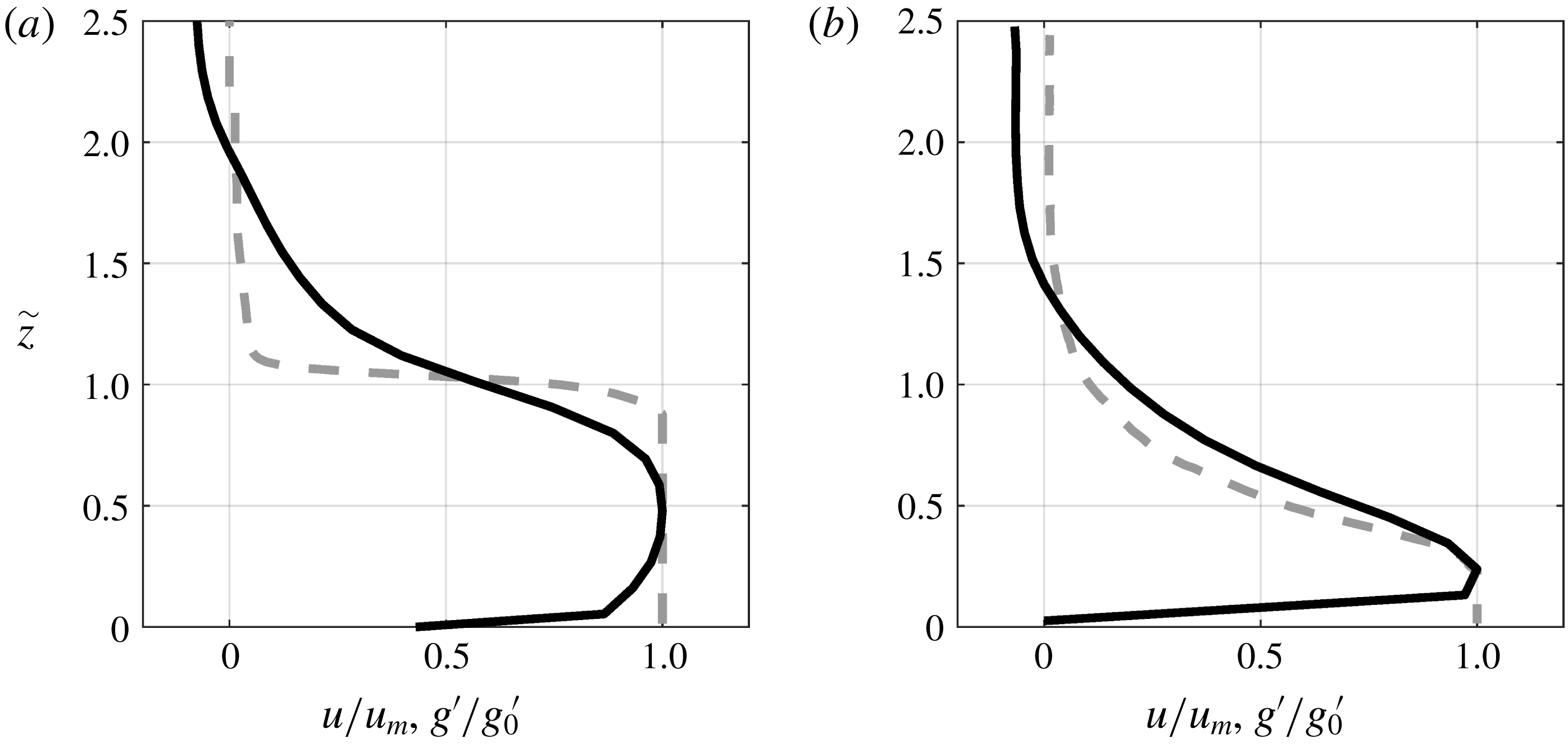
Gravity currents are often modelled by shallow water equations (Ungarish Reference Ungarish2011; Wirth Reference Wirth2011) that assume a constant layer-averaged density and velocity and which lead to an overestimation of the driving force due to the pressure gradient by 33 %, and up to 50 % depending on the chosen approximated shapes of the profiles (Pokrajac, Venuleo & Franca Reference Pokrajac, Venuleo and Franca2017). Figure 15 displays time-averaged density (dashed lines) and velocity (continuous lines) profiles for the experiment D2-7 at
 $x=-5~\text{cm}$
(a) and at
 $x=50~\text{cm}$
(b). The density and velocity profiles are close to the ‘top-hat’ shape upstream of the slope (figure 15
a) as long as the interface is stable and little mixing at the interface takes place, whereas when the shear layer develops a triangular shape is approached for both density and velocity profile. For the experiments D0 the initial velocity and density profiles are closer to the ‘top-hat’ profile. After the beginning of the KHI, both profiles are very similar for all experiments and close to the triangular profile as highlighted in figure 15(b).
Normalized density (grey dashed line) and velocity profiles (black line), upstream of the slope (a), at the end of the observed slope (b) for the experiment D2-7.

The shape factors introduced by Ellison & Turner (Reference Ellison and Turner1959) allow us to take into account the deviation of the instantaneous velocity and density profiles from the simplified rectangular (top-hat) profile by assuming the self-similarity of these profiles, and hence to correct the shallow water solution.
The integral velocity
 $U$
and current depth
 $h$
of the current are deduced from the experimental observations by integrating the velocity profile as in (4.2c,d
) over a depth
 $h_{v}$
at which the velocity has become a percentage of the maximum velocity
 $u_{m}$
. In this paper this percentage is set to
 $8\,\%$
based on the experimental resolution of the velocity data.
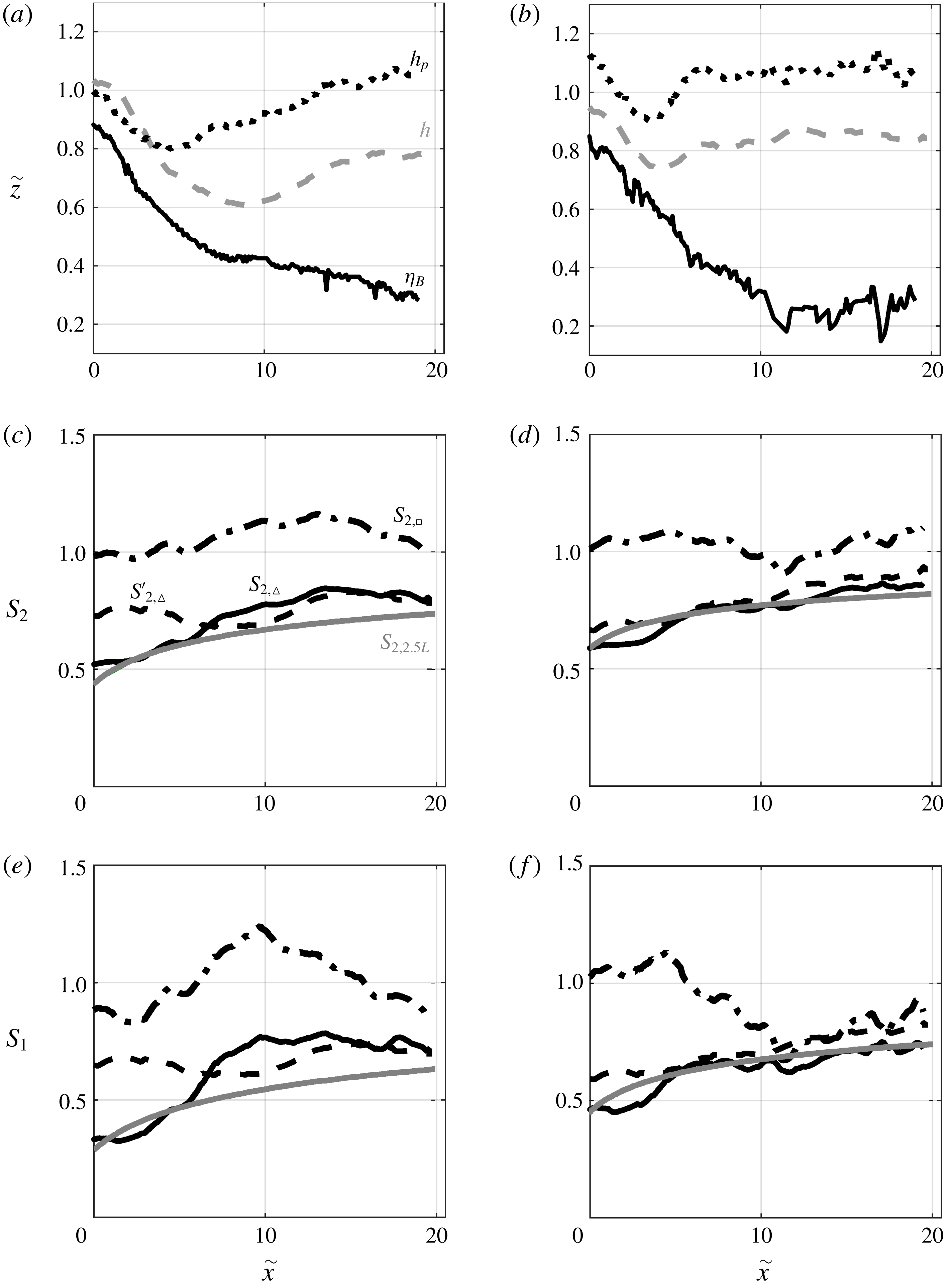
Figure 16(a,b) displays the different depths: the integral velocity layer depth
 $h$
(grey dashed line), the integral density layer depth
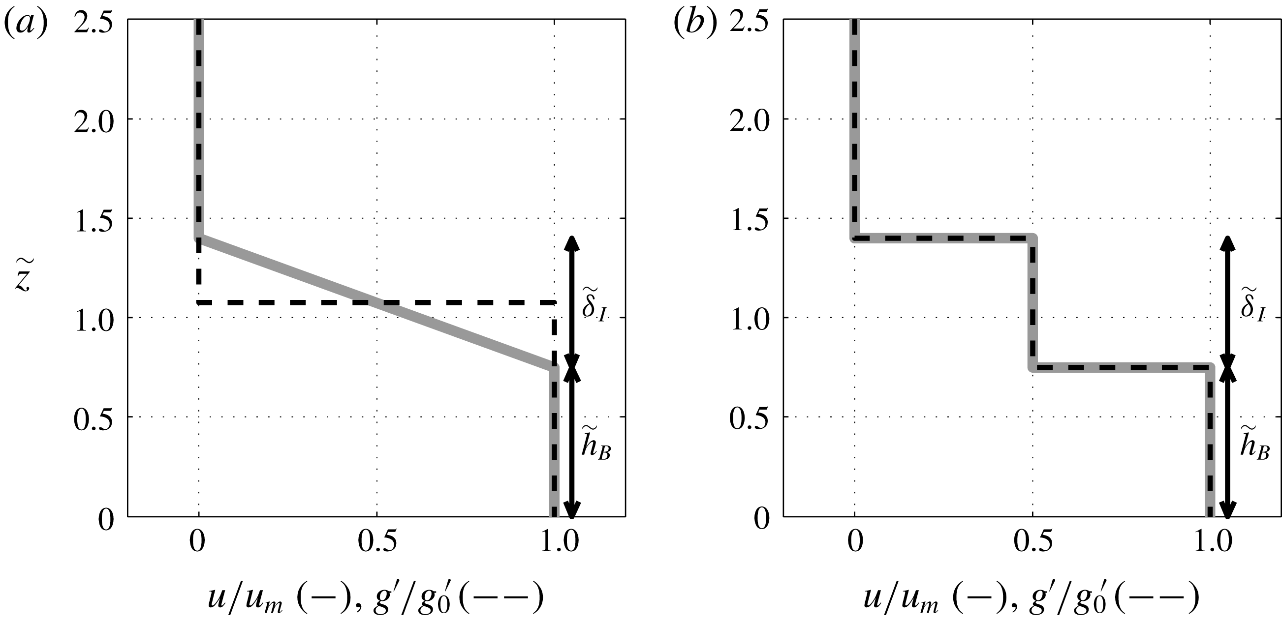
 $h_{\unicode[STIX]{x1D70C}}$
(black dotted line) and the constant maximum density layer
 $\unicode[STIX]{x1D702}_{B}$
(black continuous line) for D2-7 (a) and D1-7 (b). We see that the depth of the density layer
 $h_{\unicode[STIX]{x1D70C}}$
(dashed line in figure 16
a,b) behaves similarly to
 $h$
, while the bottom constant density layer
 $\unicode[STIX]{x1D702}_{B}$
(continuous line in figure 16
a,b) always decreases in the downstream direction to reach a thickness of a few centimetres only, thus suggesting that a triangular shape is approached moving downstream.
Integral current depth
 $h$
(grey dashed lines), constant density layer
 $\unicode[STIX]{x1D702}_{B}$
(black continuous lines), density profile height
 $h_{\unicode[STIX]{x1D70C}}$
(black dashed-dotted lines), for D2-7 (a) and D1-7 (b). Shape factors
 $S_{1}$
(c,d) and
 $S_{2}$
(e,f) for D2-7 (c,e) and D1-7 (d,f). ‘Top-hat’ density profiles with a total thickness
 $h_{\unicode[STIX]{x1D70C}}-\unicode[STIX]{x1D702}_{I}/2$
(black dotted lines), triangular density profiles (black lines), no assumption on the velocity profile, assuming both triangular density and velocity profiles (black dashed lines) and using the 2.5 layer model (continuous grey lines).

Using (4.2c,d
) and assuming a ‘top-hat’ density profile with a constant reduced gravity
 $\overline{g}^{\prime }$
through the depth
 $h_{\unicode[STIX]{x1D70C}}$
, we get the following relations for
 $S_{1}$
and
 $S_{2}$
:
 $$\begin{eqnarray}S_{1}=\frac{g^{\prime }}{\overline{g}^{\prime }}\left(\frac{h_{\unicode[STIX]{x1D70C}}}{h}\right)^{2},\quad S_{2}=\frac{g^{\prime }}{\overline{g}^{\prime }}\frac{h_{\unicode[STIX]{x1D70C}}}{h}.\end{eqnarray}$$
The corresponding shape factors assuming a triangular shape of the density profile are obtained multiplying the above values of
 $S_{1}$
and
 $S_{2}$
by
 $1/3$
and
 $1/2$
, respectively.
The shape factors estimated using ‘top-hat’ and triangular shapes of the density profile and no assumption on the velocity profile are illustrated in figure 16(c–f) using dash-dotted and continuous lines, respectively. In the ‘top-hat’ case, the factors are both of
 $O(1)$
over the full distance considered with standard deviations of
 $0.12$
and
 $0.05$
for
 $S_{1}$
and
 $S_{2}$
, respectively, larger for
 $S_{1}$
because of the squared relation in (B 1). The constant value around one for this shape confirms that the pressure and gravity terms are overestimated in this case. Using triangular shapes, the values start from
 $0.3{-}0.5$
for
 $S_{1}$
and
 $0.55{-}0.7$
for
 $S_{2}$
at
 $\tilde{x}=0$
and increase in downstream direction to reach finally values of approximately
 $0.7$
for
 $S_{1}$
and
 $0.75{-}0.9$
for
 $S_{2}$
at
 $\tilde{x}=20$
for both experiments, in accord with the observed development of the velocity and density profiles of the gravity flow.
So far, no assumption has been made on the shape of the velocity profile. If it is assumed, for example, that the velocity and density profiles are both triangular with a height
 $h_{\unicode[STIX]{x1D70C}}=h_{v}=(4/3)h$
, the shape factors
 $S_{1}$
and
 $S_{2}$
become
 $$\begin{eqnarray}S_{1}=\frac{16}{27}\frac{g_{0}^{\prime }}{\overline{g}^{\prime }}\quad \text{and}\quad S_{2}=\frac{2}{3}\frac{g_{0}^{\prime }}{\overline{g}^{\prime }},\end{eqnarray}$$
and
 $S_{3}$
can be estimated by assuming
 $u=u_{m}(1-z/h_{v})$
from which follows (cf. equations (4.2c,d
)):
 $U=2/3u_{m}$
,
 $h=3/4h_{v}$
and
 $S_{3}=2/3$
. The shape factors obtained using triangular profiles for both the density and velocity profiles are represented in figure 16(c–f) by the dashed lines. They differ from the continuous lines, where no assumption on the velocity profile has been made, in the first developing region (
 $0<\tilde{x}<5$
), but vary similarly for
 $\tilde{x}>5$
.
Definition sketch of the velocity (grey line) and reduced gravity profiles (black dashed line) (a) in a two-layer SW model and (b) in the 2.5-layer model.

An alternative way to estimate the shape factors, which is more sophisticated than considering a two-layer system, as is the case in the SW model, is to take into account an additional layer of thickness
 $\unicode[STIX]{x1D6FF}_{I}$
, as depicted in figure 17. The top layer is assumed quiescent and the shear layer velocity is supposed to be half of the velocity of the bottom layer, but the model can be easily extended to any other ratio between the velocities in the shear and bottom layer. Similarly, the density is assumed to be half of the density of the bottom layer in the sheared velocity layer, and constant, but the approach can be adapted to other interface configurations. Neglecting the drag terms we have,
 $$\begin{eqnarray}\displaystyle & \displaystyle \frac{\text{d}\tilde{u} _{m}^{2}}{\text{d}\tilde{x}}+2\frac{\text{d}}{\text{d}\tilde{x}}\left(\tilde{h}_{B}+\frac{\tilde{\unicode[STIX]{x1D6FF}}_{I}}{2}\right)\cos \unicode[STIX]{x1D703}=2\sin \unicode[STIX]{x1D703}, & \displaystyle\end{eqnarray}$$
 $$\begin{eqnarray}\displaystyle & \displaystyle \frac{\text{d}\tilde{q}_{B}}{\text{d}\tilde{x}}=0, & \displaystyle\end{eqnarray}$$
 $$\begin{eqnarray}\displaystyle & \displaystyle \frac{\text{d}\tilde{q}_{I}}{\text{d}\tilde{x}}=0, & \displaystyle\end{eqnarray}$$
 $\tilde{u} _{m}=u_{m}/{\mathcal{U}}$
corresponds to the dimensionless maximum free-stream velocity,
 $\tilde{h}_{B}=h_{B}/{\mathcal{L}}$
is the dimensionless bottom layer thickness,
 $\tilde{q}_{B}=q_{B}/q_{0}=\tilde{u} _{m}\tilde{h}_{B}$
and
 $\tilde{q}_{I}=q_{I}/q_{0}=\tilde{u} _{m}\tilde{\unicode[STIX]{x1D6FF}}_{I}/2$
. The unknowns are
 $\tilde{u} _{m}$
,
 $\tilde{h}_{B}$
and
 $\tilde{\unicode[STIX]{x1D6FF}}_{I}$
. Equation (B 3a
) can be analytically solved to give the implicit solution,
 $$\begin{eqnarray}\tilde{u} _{m}^{2}+2\left(\tilde{h}_{B}+\frac{\tilde{\unicode[STIX]{x1D6FF}}_{I}}{2}\right)\cos \unicode[STIX]{x1D703}=2\tilde{x}\sin \unicode[STIX]{x1D703}+\unicode[STIX]{x1D701},\quad \text{with }\unicode[STIX]{x1D701}=\tilde{u} _{m0}^{2}+2\left(\tilde{h}_{B0}+\frac{\tilde{\unicode[STIX]{x1D6FF}}_{I0}}{2}\right)\cos \unicode[STIX]{x1D703},\end{eqnarray}$$
where
 $\tilde{u} _{m0}$
and
 $\tilde{h}_{B0}$
are estimated using the initial condition
 $F^{2}=1$
and are linked to
 $\tilde{U} _{0}$
and
 $\tilde{h}_{0}$
through Turner’s integrals (4.2.a,b
),
 $$\begin{eqnarray}\displaystyle & \displaystyle \tilde{u} _{m0}=\unicode[STIX]{x1D712}_{0}\tilde{U} _{0}, & \displaystyle\end{eqnarray}$$
 $$\begin{eqnarray}\displaystyle & \displaystyle \tilde{h}_{B0}+\tilde{\unicode[STIX]{x1D6FF}}_{I0}/2=\unicode[STIX]{x1D712}_{0}^{-1}\tilde{h}_{0}, & \displaystyle\end{eqnarray}$$
 $$\begin{eqnarray}\displaystyle & \displaystyle \unicode[STIX]{x1D712}_{0}=\frac{\tilde{h}_{B0}+\tilde{\unicode[STIX]{x1D6FF}}_{I0}/2}{\tilde{h}_{B0}+\tilde{\unicode[STIX]{x1D6FF}}_{I0}/4}. & \displaystyle\end{eqnarray}$$
 $\unicode[STIX]{x1D712}_{0}$
links Turner’s variables (
 $\tilde{U} ,\tilde{h}$
) to the free-stream layer variables (
 $\tilde{u} _{m},\tilde{h}_{B}$
). Combining (B 5b
) and (B 5c
) we get
 $\unicode[STIX]{x1D712}_{0}=2(\tilde{h}_{0}-\sqrt{\tilde{h}_{0}^{2}-\tilde{h}_{0}\tilde{\unicode[STIX]{x1D6FF}}_{I0}})/\tilde{\unicode[STIX]{x1D6FF}}_{I0}$
.
The shape factors can now be obtained as
 $S_{1}=\unicode[STIX]{x1D712}^{-2}(g_{0}^{\prime }/\overline{g}^{\prime })$
and
 $S_{2}=\unicode[STIX]{x1D712}^{-1}(g_{0}^{\prime }/\overline{g}^{\prime })$
and are represented in figure 16(c–f) by the grey continuous lines. We see that
 $S_{1}=0.56{-}0.87$
and
 $S_{2}=0.75{-}0.93$
. The so obtained values will be finally used to solve the system (4.1) since they are the most representative, considering both the shear layer thickness and the bottom layer, and are also shown to produce better agreement when comparing the numerical solution with the experimental data as in § 7.