1 Introduction
Strong free-surface turbulence (SFST) leads to significant interactions between gas and liquid, resulting in surface phenomena not observed in weak free-surface turbulence (WFST) (Brocchini & Peregrine Reference Brocchini and Peregrine2001a ). When SFST is energetic enough to overcome the stabilizing effects of gravity and surface tension, the free surface becomes strongly distorted, resulting in (steep) surface waves, projections, dimples and finally surface breakup. The surface breakup creates complex two-phase gas–liquid mixtures such as drops and bubbles near the interface, resulting in measurable air entrainment. The study of SFST, the turbulence characteristics near a highly distorted free surface and the air entrainment driven by SFST are of fundamental scientific interest. With recent interest in modelling the white bubbly water in ship wakes, SFST and SFST air entrainment are also of practical importance to the design and analysis of modern surface vessels.
Brocchini & Peregrine (Reference Brocchini and Peregrine2001a
) described a wide range of free surface deformations when turbulence exists in the bulk liquid near the free surface (neglecting dynamic effects of the gas). By considering the stabilizing effects of gravity and surface tension against the free-surface disturbance due to turbulence, they defined different flow regimes in which the free surface exhibits distinct features. When turbulence is sufficiently strong, neither gravity nor surface tension can maintain the cohesion of the surface, resulting in droplets and air entrainment. This near-surface two-phase flow regime or the ‘strong turbulence regime’ occurs under large Froude (
 $Fr$
) and Weber (
 $We$
) numbers. On the other hand, when turbulence is relatively weak, the free surface remains nearly flat due to the stabilizing effect of either gravity or surface tension. This regime or the ‘weak turbulence regime’ corresponds to small Froude or Weber numbers.
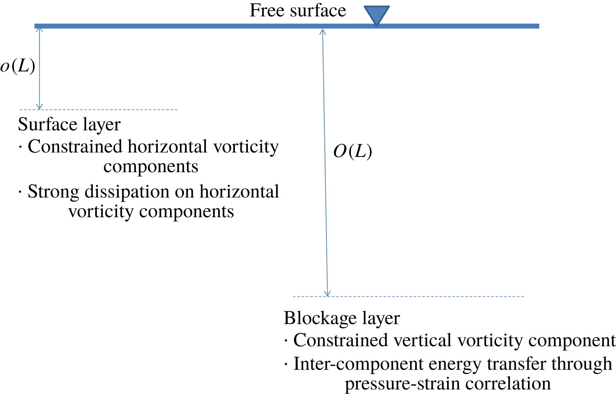
Many studies on WFST in the weak turbulence regime have been performed numerically (Handler et al. Reference Handler, Swean, Leighton and Swearingen1993; Borue, Orszag & Staroselsky Reference Borue, Orszag and Staroselsky1995; Pan & Banerjee Reference Pan and Banerjee1995; Walker, Leighton & Garza-Rios Reference Walker, Leighton and Garza-Rios1996; Nagaosa Reference Nagaosa1999; Shen et al. Reference Shen, Zhang, Yue and Triantafyllou1999; Fulgosi et al. Reference Fulgosi, Lakehal, Banerjee and De Angelis2003; Guo & Shen Reference Guo and Shen2010; Yamamoto & Kunugi Reference Yamamoto and Kunugi2011) and experimentally (Walker, Chen & Willmarth Reference Walker, Chen and Willmarth1995; Smolentsev & Miraghaie Reference Smolentsev and Miraghaie2005; Savelsberg & van de Water Reference Savelsberg and van de Water2008, Reference Savelsberg and van de Water2009). Hunt, Stretch & Belcher (Reference Hunt, Stretch and Belcher2011) performed a linearized rapid-distortion analysis to investigate viscous coupling of turbulence at a nearly flat interface. In WFST, the (almost) flat free surface has a large blockage effect, which strongly constrains the liquid movements normal to the surface, resulting in a blockage layer wherein horizontal velocity fluctuations are enhanced at the expense of vertical velocity fluctuations. Closer to the free surface, where the dynamic boundary condition of (almost) zero stress is felt, a thinner surface layer characterized by fast variations of the horizontal vorticity components appears. The characteristic thicknesses and features of these two layers are summarized in figure 1 according to Shen et al. (Reference Shen, Zhang, Yue and Triantafyllou1999). As expected, no air entrainment occurs in the weak turbulence regime.
Schematic of the inner surface and outer blockage layers in WFST according to Shen et al. (Reference Shen, Zhang, Yue and Triantafyllou1999), where
 $L$
is the characteristic length scale.

In the strong turbulence regime with large
 $Fr$
and
 $We$
, Brocchini & Peregrine (Reference Brocchini and Peregrine2001a
) pointed out that the surface blockage effect is significantly reduced due to the weak effects of gravity and surface tension. Therefore, turbulence near the free surface shows qualitatively different characteristics between WFST and SFST. Significantly, SFST is accompanied by large surface deformations, surface breakup/breaking, formation of liquid droplets and sprays and entrainment of air cavities and bubbles. Compared to WFST, there exists little research on SFST in the strong turbulence regime. Hong & Walker (Reference Hong and Walker2000), Brocchini & Peregrine (Reference Brocchini and Peregrine2001b
) and Brocchini (Reference Brocchini2002) derived a set of Reynolds-averaged governing equations and averaged boundary conditions for SFST. Mortazavi et al. (Reference Mortazavi, Le Chenadec, Moin and Mani2016) performed direct numerical simulations (DNS) of a turbulent hydraulic jump where they found that the energy spectrum of near-surface turbulence approximately follows the Kolmogorov spectrum with a power law of
 $k^{-5/3}$
, where
 $k$
is wavenumber. Murzyn, Mouaze & Chaplin (Reference Murzyn, Mouaze and Chaplin2007) and Chachereau & Chanson (Reference Chachereau and Chanson2011) performed experimental studies on air entrainment in hydraulic jumps. They observed that air entrainment happens as
 $Fr$
becomes larger than a critical value. They also found that the volume of air entrainment increases with increasing
 $Fr$
. Chanson & Toombes (Reference Chanson and Toombes2003) measured the chord length of entrained bubbles in a supercritical open channel flow down a cascade. For bubble chord lengths greater than a critical scale, their results (re-plotted in log–log scale) show a probability density function that appears to follow a power law. Garrett, Li & Farmer (Reference Garrett, Li and Farmer2000), Deane & Stokes (Reference Deane and Stokes2002), Wang, Yang & Stern (Reference Wang, Yang and Stern2016) and Deike, Melville & Popinet (Reference Deike, Melville and Popinet2016) studied the bubbles inside breaking waves and observed that the bubble size spectrum is proportional to
 $r^{-10/3}$
. Garrett et al. (Reference Garrett, Li and Farmer2000) proposed a cascade scenario to understand the power law.
In this study, we choose a simple canonical free-surface turbulence (FST) flow with turbulent kinetic energy supplied by an underlying near-surface shear flow. The physical problem is the same as that considered in WFST in the limit of small Froude number and infinite Weber number (studied numerically by Shen et al.
Reference Shen, Zhang, Yue and Triantafyllou1999; Shen, Triantafyllou & Yue Reference Shen, Triantafyllou and Yue2000; Shen & Yue Reference Shen and Yue2001; Liu et al.
Reference Liu, Kermani, Shen and Yue2009). Our interest is to extend this to the SFST regime characterized by large
 $Fr$
and
 $We$
. We perform DNS of three-dimensional two-phase (air and water) viscous turbulent flow for this problem using the volume conserving volume-of-fluid method (cVOF) (Weymouth & Yue Reference Weymouth and Yue2010). The DNS is performed for over ranges of
 $Fr$
and
 $We$
to elucidate the dependence of FST and air entrainment on these parameters. Our main interests are to: (i) elucidate the characteristics of turbulence in SFST compared to that in WFST; (ii) obtain the size distribution of the entrained bubbles and its evolution as the entrainment process continues; (iii) quantify the amount of air entrainment in SFST and its dependence on
 $Fr$
and
 $We$
.
We perform systematic DNS over a range of
 $Fr$
and
 $We$
to show the characteristics of near-surface turbulence in SFST. We find that for sufficiently large
 $Fr$
and
 $We$
, the blockage layer and surface layer observed in WFST disappear, with the SFST obtaining near surface isotropy and energy spectrum following the
 $k^{-5/3}$
power law. The free surface exhibits large deformations due to the strong underlying turbulence, and we quantify the average entrainment rate, as functions of
 $Fr$
and
 $We$
of the flow. We show that above some critical values of
 $Fr$
and
 $We$
(below which there is no air entrainment) the entrainment rate scales as
 $Fr^{2}$
or
 $We$
depending on whether gravity or surface tension dominates in the bubble formation process. We also characterize the size distributions of the entrained bubbles. We find that the bubble size spectrum follows a power-law size spectrum
 $N_{a}(r)\propto r^{-10/3}$
in the early phase of the entrainment process. This scaling law is obtained using a simple energy argument. With continuing air entrainment and ongoing turbulence fragmentation of the (already) entrained bubbles, the bubble size spectrum starts to evolve with time and deviate from the initial power law. To provide some qualitative insight into this evolution, we suggest a heuristic model which combines the two main mechanisms of ongoing SFST entrainment and subsequent fragmentation cascades of these bubbles.
This paper is organized as follows. Section 2 presents the governing equations and numerical method used in this study. Section 3 contains the problem definition and establishes the appropriate resolution of the numerical simulations. Section 4 describes the turbulence characteristics specific to SFST in contrast to WFST. Section 5 investigates air entrainment and the bubble size distribution of entrained bubbles in SFST. Section 6 performs a systematic study of both
 $Fr$
and
 $We$
and discusses their effects on air entrainment. Section 7 contains the conclusions.
2 Methodology
2.1 Numerical implementations
We perform high-resolution DNS by solving the three-dimensional two-phase incompressible Navier–Stokes equations with a fully nonlinear interface. We assume atmospheric conditions and do not consider the solubility of air (and other chemical reactions). The three-dimensional two-phase incompressible Navier–Stokes equations in a single-fluid form with variable density
 $\unicode[STIX]{x1D70C}$
and viscosity
 $\unicode[STIX]{x1D707}$
are,
 $$\begin{eqnarray}\left.\begin{array}{@{}c@{}}\displaystyle \frac{\unicode[STIX]{x2202}\boldsymbol{u}}{\unicode[STIX]{x2202}t}+\unicode[STIX]{x1D735}\boldsymbol{\cdot }(\boldsymbol{u}\boldsymbol{u})=-\frac{1}{\unicode[STIX]{x1D70C}}\unicode[STIX]{x1D735}p+\frac{1}{\unicode[STIX]{x1D70C}Re}\unicode[STIX]{x1D735}\boldsymbol{\cdot }\unicode[STIX]{x1D707}(\unicode[STIX]{x1D735}\boldsymbol{u}+\unicode[STIX]{x1D735}\boldsymbol{u}^{\text{T}})+\frac{\boldsymbol{e}_{z}}{Fr^{2}}+\frac{1}{We}\unicode[STIX]{x1D705}\unicode[STIX]{x1D6FF}_{s}\boldsymbol{n},\\ \displaystyle \unicode[STIX]{x1D735}\boldsymbol{\cdot }\boldsymbol{ u}=0,\\ \displaystyle \frac{\unicode[STIX]{x2202}f}{\unicode[STIX]{x2202}t}+\boldsymbol{u}\boldsymbol{\cdot }\unicode[STIX]{x1D735}f=0,\end{array}\right\}\end{eqnarray}$$
where
 $f(\boldsymbol{x},t)$
represents the volume fraction implemented by the conservative volume-of-fluid method (cVOF) (Weymouth & Yue Reference Weymouth and Yue2010). In (2.1), the density and viscosity are defined as
 $\unicode[STIX]{x1D70C}(f)=f+(1-f)\unicode[STIX]{x1D70C}_{2}/\unicode[STIX]{x1D70C}_{1}$
,
 $\unicode[STIX]{x1D707}(f)=f+(1-f)\unicode[STIX]{x1D707}_{2}/\unicode[STIX]{x1D707}_{1}$
, where
 $\unicode[STIX]{x1D70C}_{1}$
,
 $\unicode[STIX]{x1D70C}_{2}$
and
 $\unicode[STIX]{x1D707}_{1}$
,
 $\unicode[STIX]{x1D707}_{2}$
denote the density and viscosity of the two fluids respectively, and
 $\boldsymbol{u}$
is the velocity field,
 $\boldsymbol{e}_{z}$
denotes a unit vector in vertical direction,
 $\unicode[STIX]{x1D6FF}_{s}$
is the interfacial Dirac delta function,
 $\unicode[STIX]{x1D705}$
is the interface curvature and
 $\boldsymbol{n}$
is the normal vector to the interface. The equation is non-dimensionalized by characteristic velocity scale
 $U$
and length scale
 $L$
and the water density
 $\unicode[STIX]{x1D70C}_{1}$
and viscosity
 $\unicode[STIX]{x1D707}_{1}$
such that the relevant parameters of the problem are Reynolds number
 $Re=\unicode[STIX]{x1D70C}_{1}UL/\unicode[STIX]{x1D707}_{1}$
, Froude number
 $Fr=U/\sqrt{gL}$
and Weber number
 $We=\unicode[STIX]{x1D70C}_{1}U^{2}L/\unicode[STIX]{x1D70E}$
(using the surface tension coefficient
 $\unicode[STIX]{x1D70E}$
).
The numerical implementation of (2.1) is a second-order (in space and time) finite volume scheme, with a sharp interface, utilizing a staggered grid. Time integration is a two-stage Runge–Kutta method. A projection method is used to conserve mass and solve for the pressure. The resulting variable coefficient Poisson equation is solved using the HYPRE library (Falgout & Yang Reference Falgout and Yang2002; Falgout, Jones & Yang Reference Falgout, Jones and Yang2006). Finally, surface tension effects are implemented through the continuous surface force (CSF) method (Brackbill, Kothe & Zemach Reference Brackbill, Kothe and Zemach1992) along with a height-function method for the interface curvature calculation described in Popinet (Reference Popinet2009). Details of the formulation and validations of the numerical method are available in Campbell (Reference Campbell2015).
A cavity identification algorithm based on the union-find algorithm (Cormen et al.
Reference Cormen, Leiserson, Rivest and Stein2009) identifies entrained air bubbles. In this scheme we define instantaneous air entrainment as the void fraction not connected to the air domain. The total entrainment volume
 $V$
is the sum of the air entrainment void fraction identified. Individual air bubbles are disjoint subsets of the entrained void fraction. The union-find algorithm has been widely used for disjoint-set data structures and takes
 $O$
(n) time in the worst case. For the problem we consider, the total void fraction is small (
 ${\lesssim}1\,\%$
), and a precise quantification of entrained volume is essential. To this end, the cVOF we use is shown to conserve volume to machine accuracy (Weymouth & Yue Reference Weymouth and Yue2010). With the cavity identification algorithm, the bubble size spectrum
 $N_{a}(r)$
of the entrained bubbles in the computational domain is calculated in terms of the equivalent spherical radius
 $r$
for the given volumes.
2.2 Solver verification
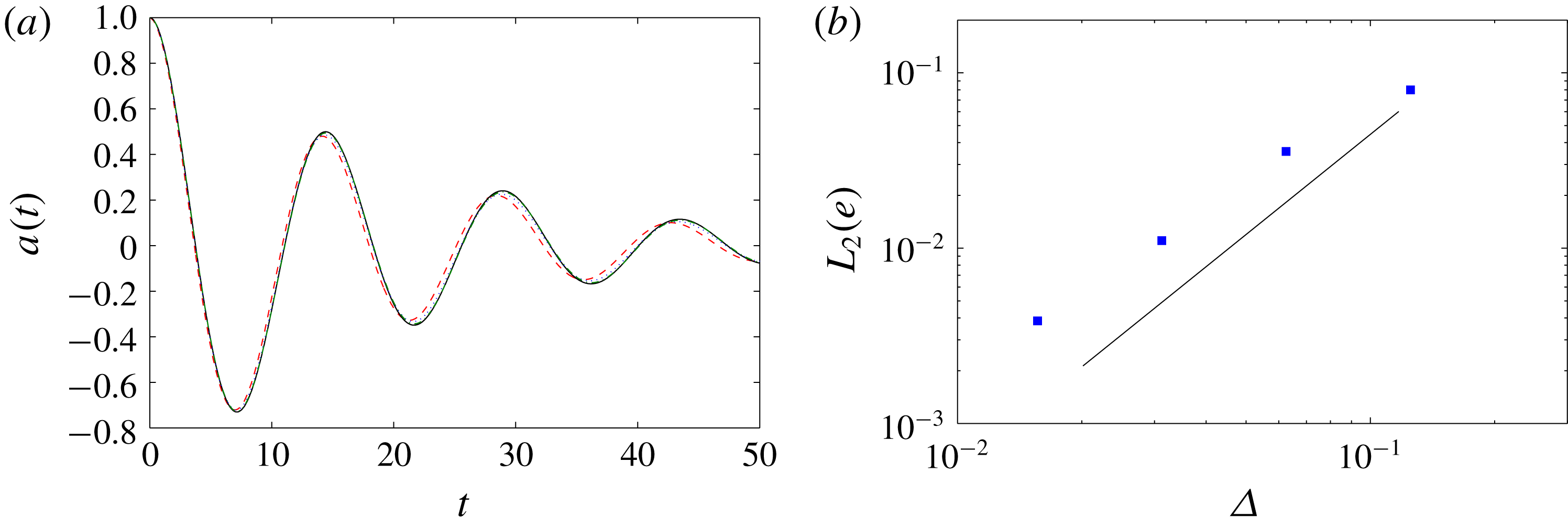
Extensive verification and validation of the solver are documented in Campbell (Reference Campbell2015). The three-dimensional Navier–Stokes solver accurately predicts turbulent wall boundary layer flows (see figure 6-1 in Campbell Reference Campbell2015). The cVOF method conserves volume to machine accuracy and is second-order accurate with respect to grid size (Weymouth & Yue Reference Weymouth and Yue2010). As surface tension is considered in this work, we validate the implementation of the surface tension by performing DNS of small amplitude standing waves driven by surface tension on the interface between two viscous fluids. The simulation results are compared with the analytical theory of Prosperetti (Reference Prosperetti1981). The solution of an interfacial standing wave has the form
 $h(x,t)=a(t)\cos (kx)$
. Here, we consider two fluids of the same constitutive properties (
 $\unicode[STIX]{x1D70C}_{1}/\unicode[STIX]{x1D70C}_{2}=1$
and
 $\unicode[STIX]{x1D707}_{1}/\unicode[STIX]{x1D707}_{2}=1$
) and
 $Re=1280$
and
 $We=550$
. The domain is a unit cube with periodic boundary conditions in the horizontal directions and no-flux boundary conditions in the vertical direction. Figure 2(a) compares the wave amplitude
 $a(t)$
of numerical simulations with the theoretical solution. Figure 2(b) shows the
 $L^{2}$
norm of the numerical error as a function of grid size
 $\unicode[STIX]{x1D6E5}$
confirming the expected second-order convergence.
(a) Time evolution of wave amplitude
 $a(t)$
at the interface of two superposed viscous fluids. ——, theoretical solution (Prosperetti Reference Prosperetti1981); – – –, numerical result with
 $32^{3}$
grids;
 $\cdot \,\cdot \,\cdot$
, with
 $64^{3}$
grids; — ⋅ —, with
 $128^{3}$
grids. (b) Error of the numerical result compared to the theoretical solution as a function of grid size. —— (thick) second-order convergence.

In § 4, the results of a simulation of a WFST case with
 $Fr^{2}=0.5$
and
 $We=\infty$
, the same case as in Shen et al. (Reference Shen, Zhang, Yue and Triantafyllou1999), will be presented. The observations and conclusions of the current simulation are consistent with those reported in Shen et al. (Reference Shen, Zhang, Yue and Triantafyllou1999). In both simulations, distinct inner/outer surface layers in WFST are identified and turbulence near the free surface is proved to be strongly anisotropic.
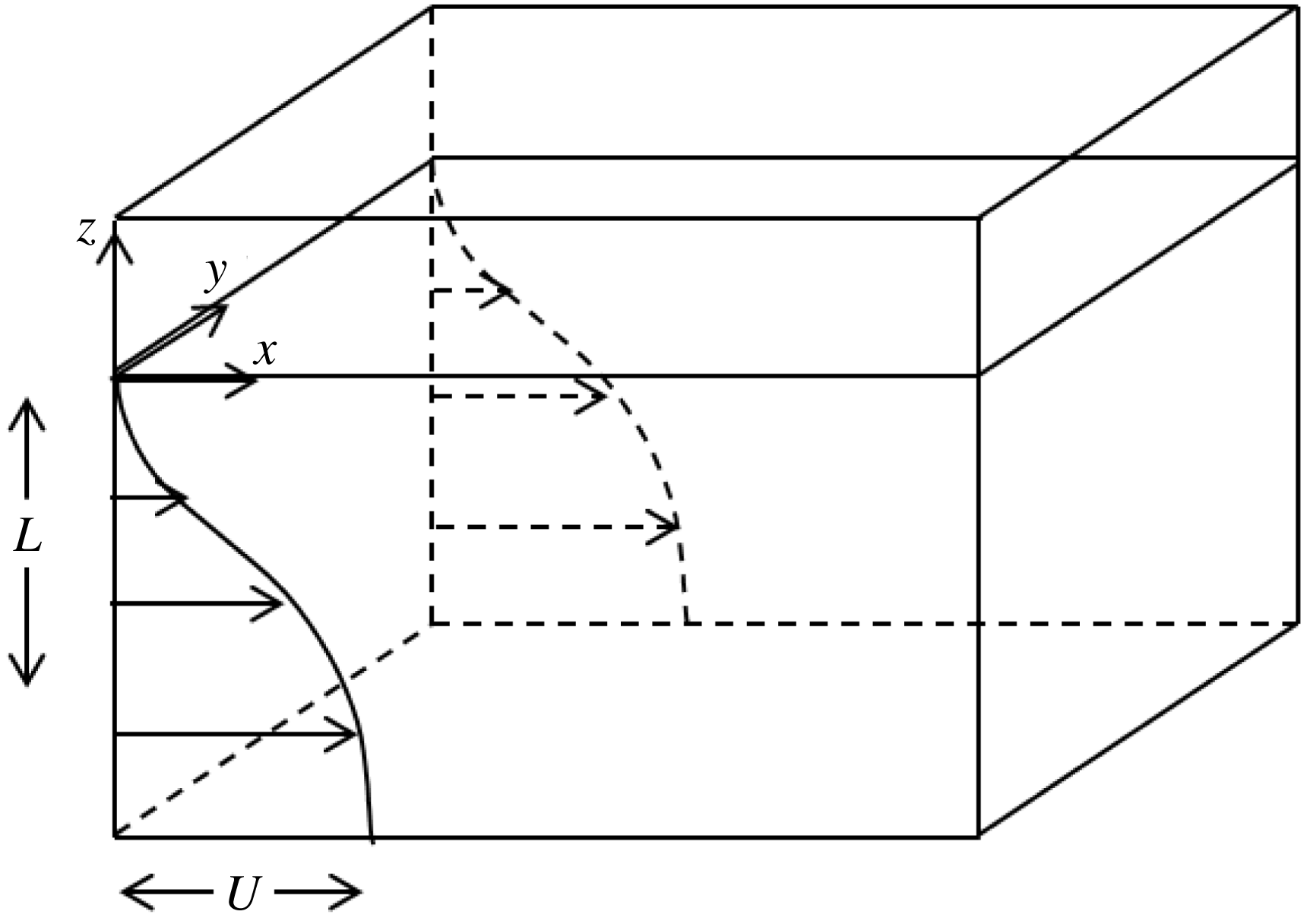
Definition sketch showing a free surface present at
 $z=0$
separating a stationary gas and a turbulent liquid with a sheared flow
 $U(z)$
, where
 $U$
is the deficit velocity and
 $L$
is the flow depth.

3 Problem definition
We consider a canonical problem of a three-dimensional incompressible two-phase (air and water) viscous turbulent flow with turbulent kinetic energy supplied by a sheared underlying bulk water flow. Figure 3 shows a definition sketch. The initial shear flow has a mean velocity profile
 $U(z,t=0)$
in the
 $x$
-direction given by (Mattingly & Criminale Reference Mattingly and Criminale1972):
 $$\begin{eqnarray}U(z/L,t=0)=1-0.9988\text{sech}^{2}(0.88137z/L)\mathfrak{}.\end{eqnarray}$$
This canonical shear-flow free-surface turbulence problem with the initial profile (3.1) has been used in a number of previous studies of weak free-surface turbulence e.g. Shen et al. (Reference Shen, Zhang, Yue and Triantafyllou1999, Reference Shen, Triantafyllou and Yue2000), Shen, Triantafyllou & Yue (Reference Shen, Triantafyllou and Yue2001) and Shen & Yue (Reference Shen and Yue2001). For the problem in figure 3, we choose the initial mean shear-flow depth
 $L$
as the characteristic length scale and the velocity deficit
 $U$
as the velocity scale. Hereafter, all the variables are normalized by
 $U$
and
 $L$
unless otherwise stated. The domain size is
 $10.472\times 10.472\times 6$
. The initial flat free surface is at
 $z=0$
. The water domain is
 $z\in [-4,0]$
and the air domain is
 $z\in [0,2]$
. The boundary conditions are periodic boundary in the horizontal
 $(x,y)$
plane and no-flux at the top and bottom of the domain. As in Shen et al. (Reference Shen, Zhang, Yue and Triantafyllou1999), the simulations are initialized using (3.1) with a small (isotropic) turbulence seed of magnitude of 0.08. The direct numerical simulations are continued through
 $T=Ut/L=160$
(during which time the FST develops, reaches a quasi-steady phase and has begun to decay). Our main focus in this work are the effects of
 $Fr$
and
 $We$
on FST characteristics, the associated surface deformation and resulting air entrainment. We perform simulations for a broad range of
 $Fr$
and
 $We$
to elucidate and quantify these effects. For sufficiently large
 $Re$
, the effects on the mechanisms above are less direct, and are not expected to change for moderate variations of
 $Re$
(amendable to DNS). In this study, we fix
 $Re=1000$
which provides turbulence with a sufficient inertial range (see figure 14 for example). We obtain select DNS at higher
 $Re$
which show discernible effects mainly in the smaller-scale turbulence structures, but have limited direct effect on the large-scale FST and air entrainment mechanisms.
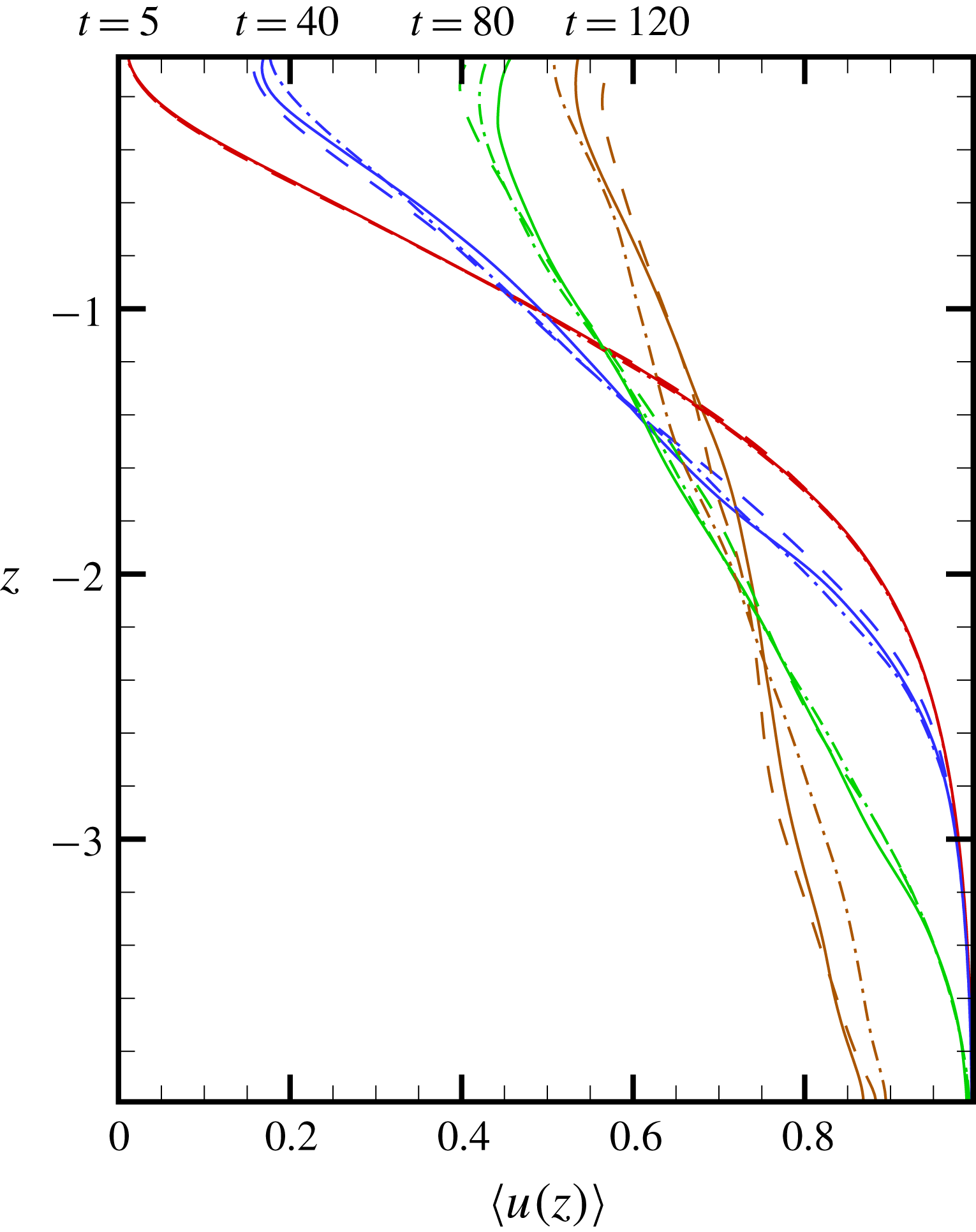
Mean velocity profile
 $\langle u(z)\rangle$
as a function of
 $z$
at different times with
 $Fr^{2}=10$
and
 $We=\infty$
. ——,
 $\unicode[STIX]{x1D6E5}_{512}$
; – – –,
 $\unicode[STIX]{x1D6E5}_{384}$
; — ⋅ —,
 $\unicode[STIX]{x1D6E5}_{256}$
.

To establish that our numerical resolution is sufficient for DNS of the problem, we consider a SFST case (
 $Fr^{2}=10$
and
 $We=\infty$
) on three different grids:
 $256^{2}\times 192$
,
 $384^{2}\times 256$
and
 $512^{2}\times 384$
with the corresponding grid sizes
 $\unicode[STIX]{x1D6E5}_{256}$
,
 $\unicode[STIX]{x1D6E5}_{384}$
,
 $\unicode[STIX]{x1D6E5}_{512}\approx 0.041$
, 0.027, 0.020. Figure 4 shows the convergence trend and general agreement of the evolution for the mean velocity profile
 $\langle u(z)\rangle$
, where
 $\langle \cdot \rangle$
denotes average in the horizontal plane, obtained using these three grids. We estimate the Kolmogorov scale based on the estimated turbulence dissipation rate
 $\unicode[STIX]{x1D716}\sim O(5\times 10^{-4})$
(see figures 21
b and 24
b). Using this value of
 $\unicode[STIX]{x1D716}$
assuming isotropic homogeneous turbulence, the Kolmogorov scale
 $\unicode[STIX]{x1D702}\sim \unicode[STIX]{x1D716}^{-1/4}Re^{-3/4}\approx 0.04$
. Thus the medium resolution grid with
 $\unicode[STIX]{x1D6E5}_{384}\approx 0.027$
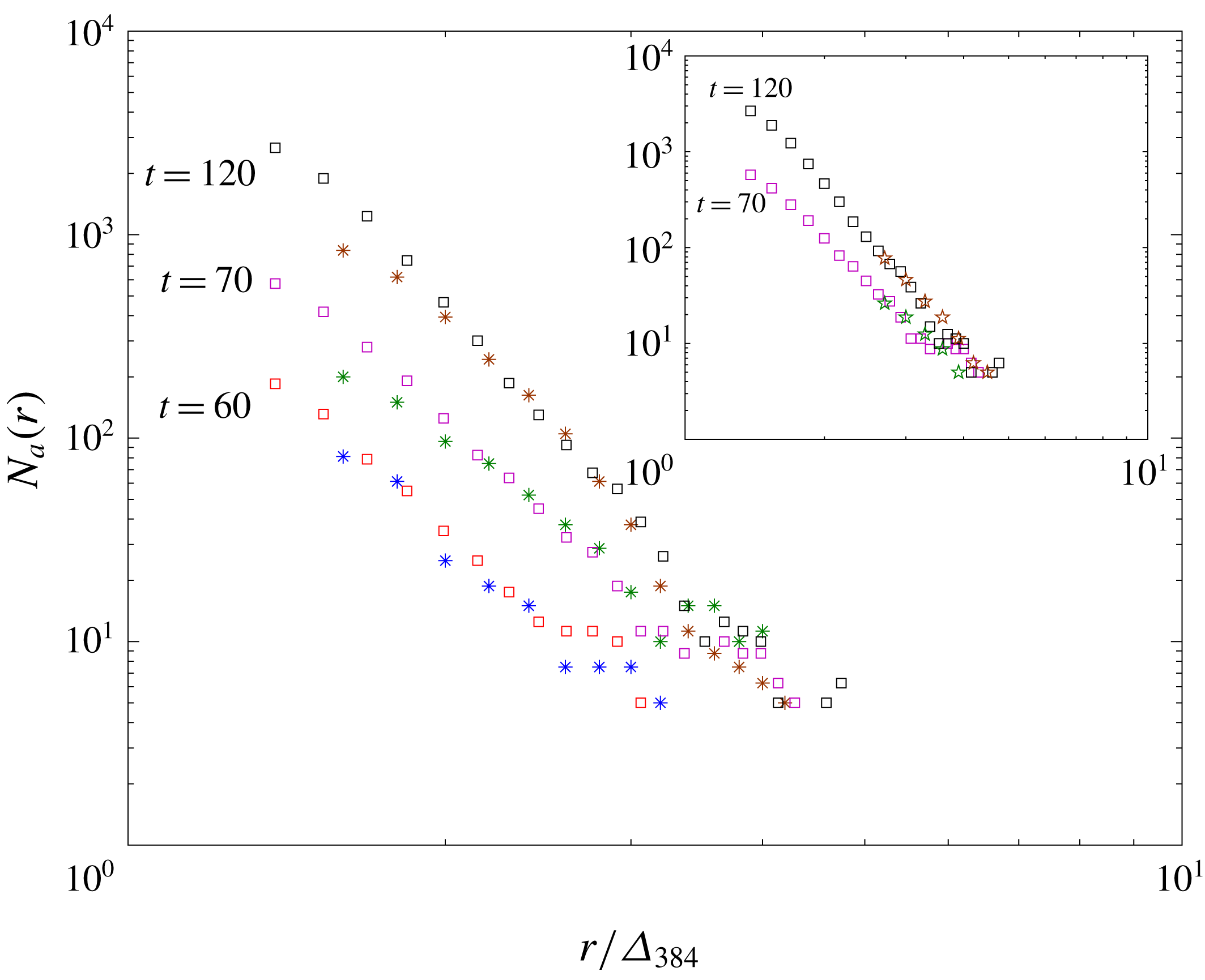
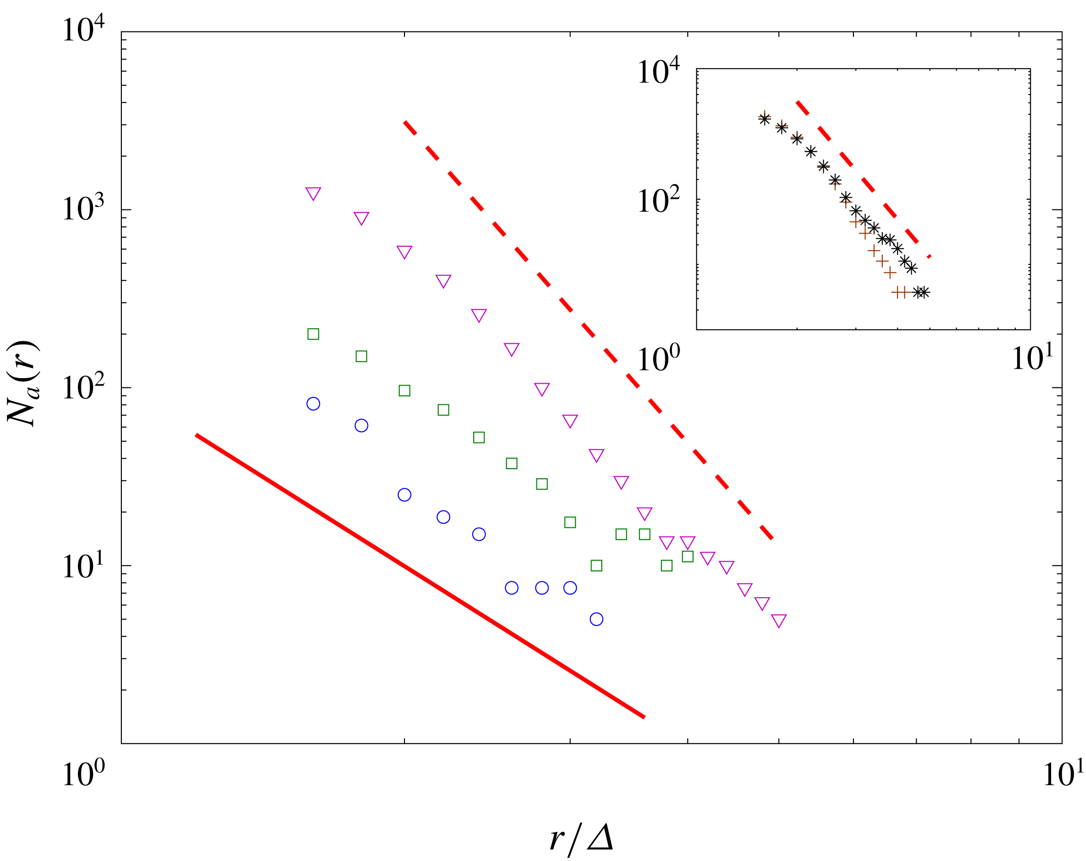
is sufficient to resolve the turbulence. Figure 5 shows the instantaneous bubble size spectrum
 $N_{a}(r)$
in the SFST with three resolutions of
 $\unicode[STIX]{x1D6E5}_{256}$
,
 $\unicode[STIX]{x1D6E5}_{384}$
and
 $\unicode[STIX]{x1D6E5}_{512}$
at different times. The shape of
 $N_{a}(r)$
and its evolution trend with time are consistent using the three resolutions, suggesting that the statistics of bubble size are converged in spite of the variation in grid size. For
 $\unicode[STIX]{x1D6E5}_{256}$
, the resolved range is relatively limited, and the results are included in an inset in figure 5. The entrained volumes are the integrals under the spectra and show similar convergence. For all the later numerical results we present, we use
 $\unicode[STIX]{x1D6E5}=\unicode[STIX]{x1D6E5}_{384}$
.
The size range of resolved bubbles depends on
 $\unicode[STIX]{x1D6E5}$
, as expected from the cVOF method. The cVOF conserves bubble volume to machine accuracy but resolves bubble sizes only to
 $\unicode[STIX]{x1D6E5}$
. Here, the smallest bubble being considered to be resolved is of radius of
 $1.5\unicode[STIX]{x1D6E5}$
. Bubbles smaller than this are not presented in our bubble size spectra. Also,
 $\unicode[STIX]{x1D6E5}$
is defined as the numerical Hinze scale. The void fraction of bubbles smaller than this scale is
 ${<}1\,\%$
of the total entrainment volume for all cases/times. Thus the entrainment rate results we report are not affected by the numerical Hinze scale.
Physically, there is a length scale
 $\ell _{\unicode[STIX]{x1D70E}}\sim O(1)~\text{mm}$
. Surface tension is important for bubbles of radii smaller than this scale and affects the bubble size spectrum accordingly (see e.g. the experimental measurements by Deane & Stokes Reference Deane and Stokes2002). Because of computational limitations of DNS, the maximum grid resolution we use is
 $L/\unicode[STIX]{x1D6E5}\approx 50$
and we are not able to resolve
 $\ell _{\unicode[STIX]{x1D70E}}$
for the case of
 $We=\infty$
. However, we point out that the presented bubble size spectra of this case are not affected by resolution of
 $\ell _{\unicode[STIX]{x1D70E}}$
. For a given (
 $L-$
based)
 $Fr$
,
 $\ell _{\unicode[STIX]{x1D70E}}/\unicode[STIX]{x1D6E5}$
decreases as
 $We$
increases. When
 $We\rightarrow \infty$
,
 $\ell _{\unicode[STIX]{x1D70E}}/\unicode[STIX]{x1D6E5}\ll 1$
. Bubbles of size below
 $\unicode[STIX]{x1D6E5}$
are not resolved, and are always excluded in the DNS bubble size spectrum. The bubbles that are included in the size spectrum are of size
 $\gg \ell _{\unicode[STIX]{x1D70E}}$
in the case of
 $We=\infty$
, indicating negligible surface tension effects on these bubbles. Physically, for bubbles of
 $r\lesssim \ell _{\unicode[STIX]{x1D70E}}$
, surface tension becomes important in the formation of these bubbles and influences the corresponding bubble size spectrum in that range. To obtain the bubble size spectrum precisely for
 $r\lesssim \ell _{\unicode[STIX]{x1D70E}}$
, extreme high resolutions, which we do not obtain, are required. In figure 5 and other figures of
 $N_{a}(r)$
hereafter,
 $r$
is scaled by
 $\unicode[STIX]{x1D6E5}$
since, for
 $We=\infty$
, physical scales associated with surface tension become
 $\ll \unicode[STIX]{x1D6E5}$
and are not useful for normalization. Instead we choose
 $\unicode[STIX]{x1D6E5}$
as a length scale to normalize
 $r$
to show the resolution used to resolve the bubbles in
 $N_{a}(r)$
.
For this SFST case, we perform an ensemble of simulations to obtain the statistical quantities of interest. Appendix A shows the validity of the obtained statistics through both an ensemble study and a statistical analysis. The maximum statistical error of the mean for all cases is less than 4 %.
Bubble size spectrum
 $N_{a}(r)$
as a function of normalized bubble radius
 $r/\unicode[STIX]{x1D6E5}_{384}$
at different times of
 $Fr^{2}=10$
and
 $We=\infty$
. ▫,
 $\unicode[STIX]{x1D6E5}_{512}$
;
 $\ast$
,
 $\unicode[STIX]{x1D6E5}_{384}$
. Inset:
 $\star$
,
 $\unicode[STIX]{x1D6E5}_{256}$
.

4 Characteristics of FST at large
 $Fr$
and
$We$


To understand quantitative differences in the turbulence characteristics between SFST and WFST, we consider a WFST case of
 $Fr^{2}=0.5$
,
 $We=\infty$
(Shen et al.
Reference Shen, Zhang, Yue and Triantafyllou1999) and a SFST case of
 $Fr^{2}=10$
,
 $We=\infty$
. The DNS are robust for
 $We\rightarrow \infty$
as well as
 $We=\infty$
. We use the latter to represent case(s) where surface tension effects are negligible compared to gravity and flow inertia. The effect of non-negligible surface tension is addressed later in § 6.2.
Time evolution of turbulent kinetic energy near the free surface
 $\frac{1}{2}\langle q^{2}\rangle _{\unicode[STIX]{x1D6FF}}$
of the flow for SFST
 $Fr^{2}=10$
,
 $We=\infty$
(- -▫- -) and WFST
 $Fr^{2}=0.5$
,
 $We=\infty$
(- -
 $\circ$
- -).

Evolution of the iso-surface of volume fraction
 $f=0.5$
for SFST with
 $Fr^{2}=10$
and
 $We=\infty$
.

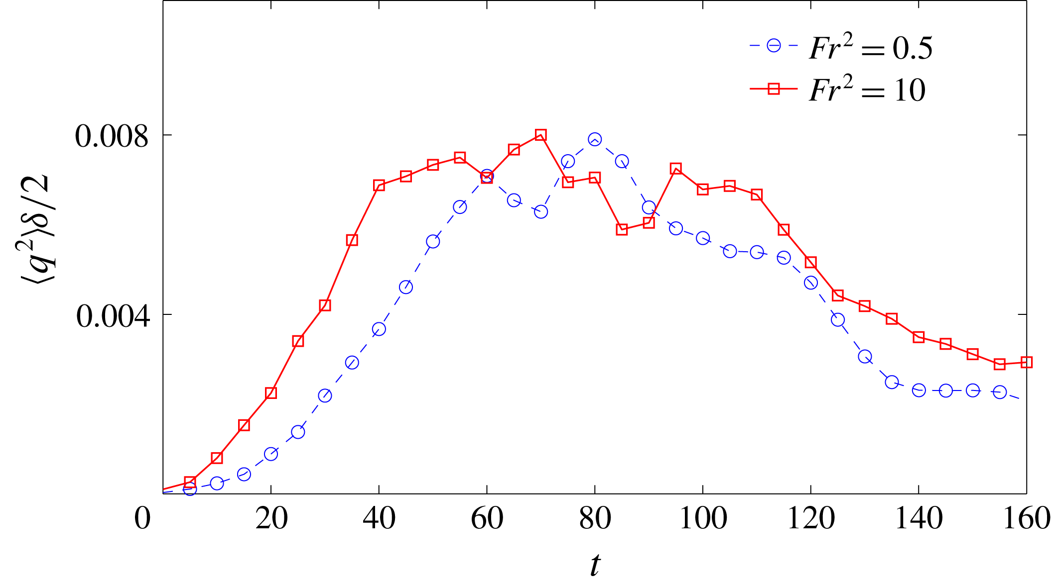
Figure 6 shows the time evolution of turbulent kinetic energy (TKE) near the free surface,
 $\frac{1}{2}\langle q^{2}\rangle _{\unicode[STIX]{x1D6FF}}$
, of the two flows, where
 $q^{2}={u^{\prime }}^{2}+{v^{\prime }}^{2}+{w^{\prime }}^{2}$
and
 $\langle \cdot \rangle _{\unicode[STIX]{x1D6FF}}$
is defined as the average over the ‘near free surface’ region.
 $u^{\prime },v^{\prime }$
and
 $w^{\prime }$
are velocity fluctuations in the
 $x$
,
 $y$
and
 $z$
directions. The detailed definition and sensitivity analysis to the parameter
 $\unicode[STIX]{x1D6FF}$
are in appendix B. The evolution of TKE shows three somewhat distinct stages for both WFST and SFST. In the initial growth stage, TKE increases due to strong production by the mean shear flow compared to turbulence dissipation. This is followed by a quasi-steady stage where production is comparable to and approximately balanced by turbulent dissipation
 $\unicode[STIX]{x1D716}$
. TKE remains remains large in this period. At later times, as the strength of the mean shear decreases (cf. figure 4), turbulence dissipation becomes dominant and TKE decays with
 $\unicode[STIX]{x1D716}$
.
This same flow has been studied extensively for WFST (Shen et al.
Reference Shen, Zhang, Yue and Triantafyllou1999, Reference Shen, Triantafyllou and Yue2000, Reference Shen, Triantafyllou and Yue2001). In particular, Shen et al. (Reference Shen, Zhang, Yue and Triantafyllou1999) showed similar TKE evolutions, and provide term-by-term analysis of the turbulent kinetic energy budget. We have performed the same analysis for the present study, detailed results omitted for brevity. The mechanism for the plateau in TKE observed here in the quasi-steady period differs from that of homogeneous shear flow where the velocity profile is maintained and the TKE reaches a non-physical plateau limited by the domain (or box) size (Rogers & Moin Reference Rogers and Moin1987). To confirm that the plateau in TKE is not due to domain size limitations, we estimate the longitudinal integral scale
 $L_{T}$
in the quasi-steady stage of the SFST case using (Pope Reference Pope2001)
 $$\begin{eqnarray}L_{T}=\int _{0}^{\infty }f(r,t)\,\text{d}r,\end{eqnarray}$$
where
 $f(r,t)=\langle u(\boldsymbol{x}+r\boldsymbol{e}_{i},t)u(\boldsymbol{x},t)\rangle /\langle u^{2}\rangle$
and
 $\boldsymbol{e}_{i}$
is the unit vector in the
 $i$
direction. At
 $t=90$
,
 $L_{T}\approx 2.5$
sampled near the free surface, which is a quarter of the horizontal computational box size;
 $L_{T}$
(with
 $\boldsymbol{e}_{i}$
in both
 $x$
and
 $y$
directions) are also checked at a number of
 $z$
locations in the bulk and confirmed to be less than half of the domain size.
The magnitude of TKE is similar in WFST and SFST (figure 21
a). In WFST, the strong blockage effect of the near flat free surface constrains the vertical component of the velocity fluctuations. Meantime, due to the existence of the flat free surface, the inter-component transfer of turbulence energy among three components results in the enhancement of the horizontal components (Shen et al.
Reference Shen, Zhang, Yue and Triantafyllou1999). Thus, the overall turbulent kinetic energy near the free surface in WFST is comparable to SFST wherein the turbulence is almost isotropic (see figure 9
c). The consequence is that, despite the notable difference in the surface deformation and air entrainment, the qualitative effect of
 $Fr$
on the available near-surface TKE is minimized (see figure 21
a). A similar conclusion is drawn for
 $We$
(see figure 24
a). This is helpful in understanding the dependence of air entrainment on
 $Fr$
and
 $We$
, and is discussed in detail in § 6.
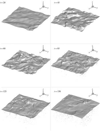
Figure 7 shows a series of images of the free surface represented by the 0.5 volume fraction (
 $f=0.5$
) iso-surface of the case SFST. During the growth stage (
 $t=20$
), the free surface is slightly deformed and this continues as turbulence further develops (
 $t=45$
), inducing large surface elevations and small-scale surface deformations. Within the quasi-steady stage (e.g.
 $t=60$
and
 $t=85$
), turbulence becomes strong enough that the surface cannot maintain its cohesion, resulting in substantial air entrainment. During the decay stage (
 $t=125$
and
 $t=150$
), the free surface becomes coherent with less distortion.
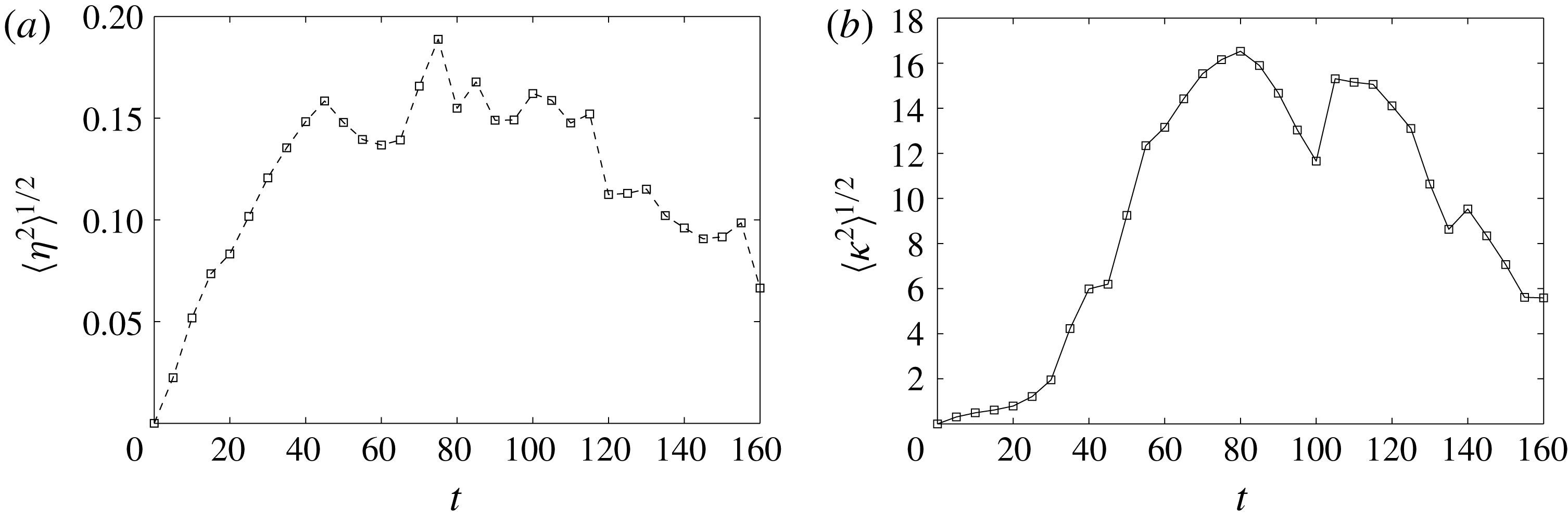
Figure 8(a,b) shows respectively the time evolution of averaged surface elevation
 $\langle \unicode[STIX]{x1D702}^{2}\rangle ^{1/2}$
and surface curvature
 $\langle \unicode[STIX]{x1D705}^{2}\rangle ^{1/2}$
. Together with the evolution of
 $\frac{1}{2}\langle q^{2}\rangle _{\unicode[STIX]{x1D6FF}}$
shown in figure 6, we observe that large surface deformation accompanies strong turbulence near the free surface. It confirms the disrupting effect of turbulence on the free surface;
 $\langle \unicode[STIX]{x1D702}^{2}\rangle ^{1/2}$
and
 $\langle \unicode[STIX]{x1D705}^{2}\rangle ^{1/2}$
for WFST are three orders of magnitude smaller than those shown in figure 8 and thus not shown. In the WFST case, the stabilizing effect of gravity on the free surface is much stronger than the disruptive effect of the turbulence and thus the surface remains nearly flat by comparison.
Time evolution of (a) averaged surface elevation
 $\langle \unicode[STIX]{x1D702}^{2}\rangle ^{1/2}$
; (b) averaged surface curvature
 $\langle \unicode[STIX]{x1D705}^{2}\rangle ^{1/2}$
for SFST of
 $Fr^{2}=10$
and
 $We=\infty$
.

Velocity fluctuation components
 $u^{\prime rms}(z)$
,
 $v^{\prime rms}(z)$
and
 $w^{\prime rms}(z)$
(a) in WFST of
 $Fr^{2}=0.5$
and
 $We=\infty$
at
 $t=90$
(b) in SFST of
 $Fr^{2}=10$
and
 $We=\infty$
at
 $t=20$
and (c) at
 $t=90$
. – – –,
 $u^{\prime rms}(z)$
; — ⋅ —,
 $v^{\prime rms}(z)$
; ——,
 $w^{\prime rms}(z)$
.

Vorticity fluctuation components
 $\unicode[STIX]{x1D714}_{x}^{\prime rms}(z)$
(– – –),
 $\unicode[STIX]{x1D714}_{y}^{\prime rms}(z)$
(— ⋅ —) and
 $\unicode[STIX]{x1D714}_{z}^{\prime rms}(z)$
(——) at time
 $t=90$
in (a) flow WFST with
 $Fr^{2}=0.5$
and
 $We=\infty$
; (b) flow SFST with
 $Fr^{2}=10$
and
 $We=\infty$
.

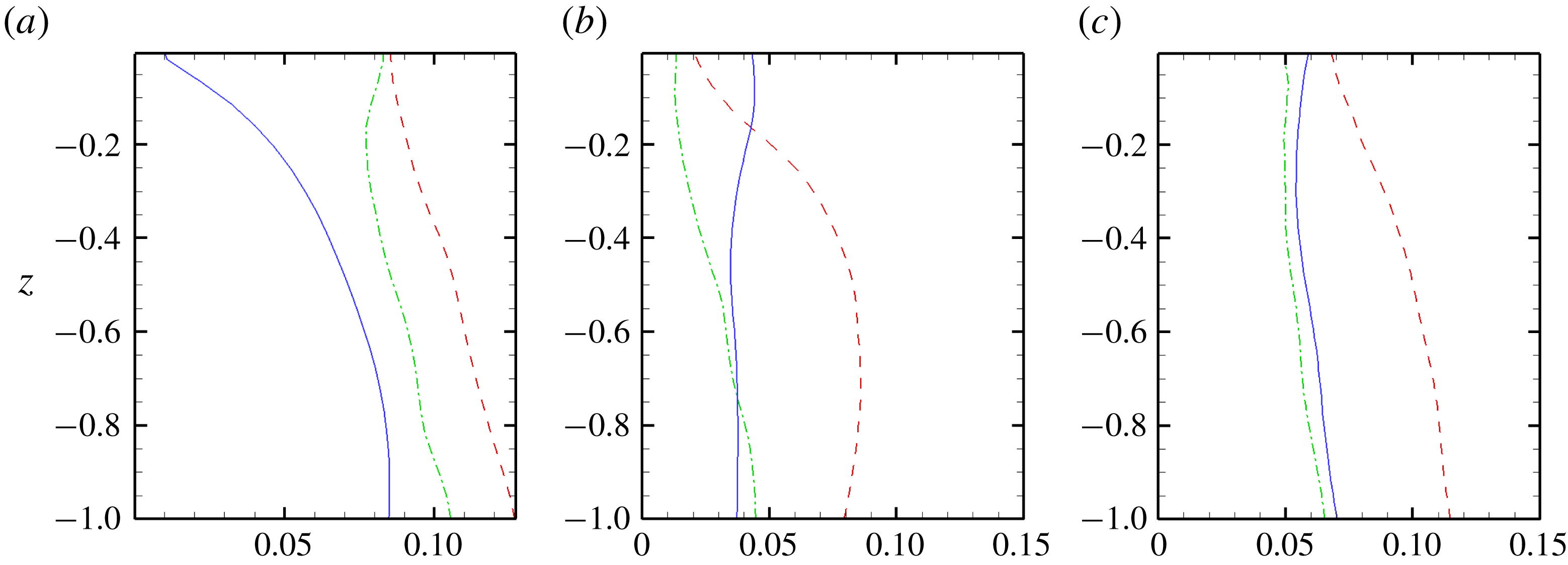
Figure 9(a) shows the vertical profiles of
 $u^{\prime rms}$
,
 $v^{\prime rms}$
and
 $w^{\prime rms}$
in the WFST flow. Consistent with Shen et al. (Reference Shen, Zhang, Yue and Triantafyllou1999), an outer blockage layer of thickness
 $O$
(0.5) is observed. In the blockage layer,
 $w^{\prime rms}$
decreases sharply approaching the free surface and becomes near zero at the free surface
 $z=0$
. Figure 9
b and figure 9
c show the profiles of
 $u^{\prime rms}$
,
 $v^{\prime rms}$
and
 $w^{\prime rms}$
of SFST at two time instances. In contrast to the WFST case, there is no sharp decrease of
 $w^{\prime rms}$
approaching the free surface, suggesting that the surface blockage effect is significantly reduced and the blockage layer disappears. In the growth stage (
 $t=20$
),
 $w^{\prime rms}$
is even larger than
 $u^{\prime rms}$
,
 $v^{\prime rms}$
at
 $z=0$
(see figure 9
b). This is due to the horizontal velocity components being constrained by the inertia of the surrounding liquid (Brocchini & Peregrine Reference Brocchini and Peregrine2001a
) in the early stage. In the quasi-steady stage (
 $t=90$
), all three components are of comparable magnitude at the free surface (see figure 9
c). Note here that in this stage,
 $u^{\prime rms}$
and
 $v^{\prime rms}$
near the free surface in SFST are smaller than those in WFST. This is because these components are enhanced due to energy transfer in the blockage layer of WFST.
Demonstration of (a) a horizontally oriented vortex structure with a ‘tube’ shape under the free surface and (b) air entrainment driven by the vortex structure. Dark: vortex structure identified by
 $\unicode[STIX]{x1D706}2$
method; Light: free-surface iso-surface of volume fraction
 $f=0.5$
.

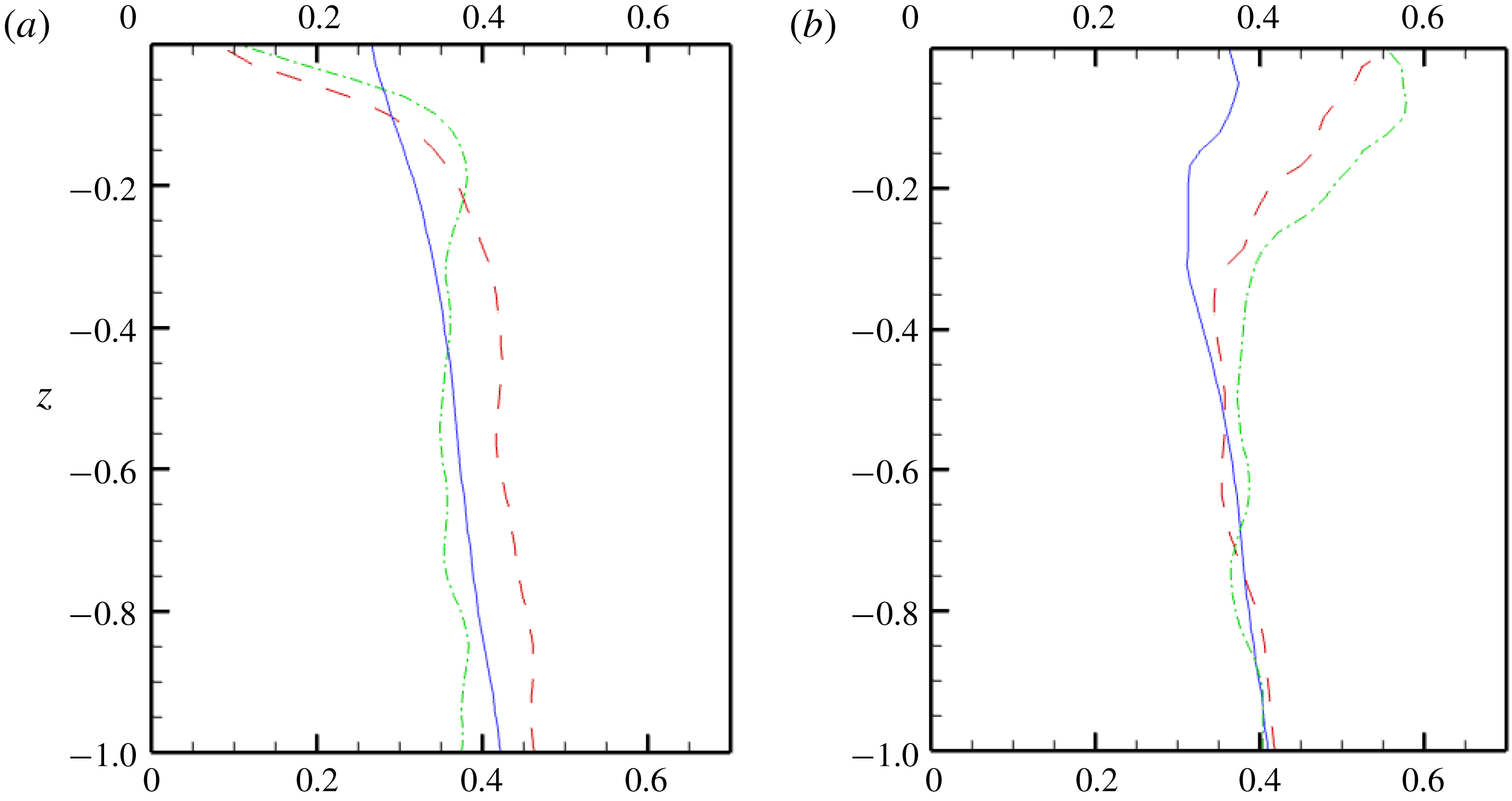
The vorticity fluctuations also show significant differences in SFST compared to WFST as shown in figure 10. In particular, the presence of the surface layer in WFST is dramatically reduced in SFST. This is seen in the horizontal vorticity components
 $\unicode[STIX]{x1D714}_{x}^{\prime rms}$
and
 $\unicode[STIX]{x1D714}_{y}^{\prime rms}$
in figure 10(a,b) for WFST and SFST, respectively. These fluctuations drop sharply over the surface layer of thickness
 $O(0.1)$
in WFST. In SFST, however,
 $\unicode[STIX]{x1D714}_{x}^{\prime rms}$
and
 $\unicode[STIX]{x1D714}_{y}^{\prime rms}$
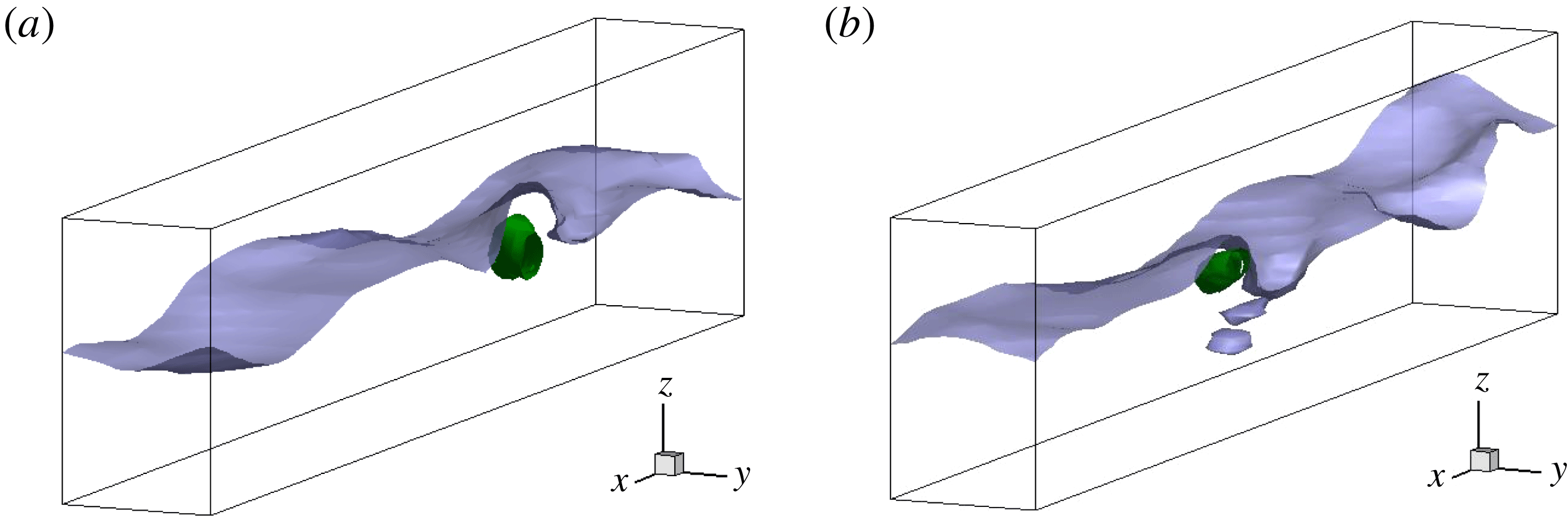
are actually enhanced due to the strong surface deformations inducing horizontally oriented coherent vortex structures. One visualization of such a vortex structure with a ‘tube’ shape is shown in figure 11. Recent studies (Yu, Hendrickson & Yue Reference Yu, Hendrickson and Yue2016; André & Bardet Reference André and Bardet2017) indeed found that the horizontally oriented vortical structure is the dominant coherent structure in FST. In addition, the main mechanism of air entrainment in FST is found to be related to the interactions of such vortex structures and the free surface. Figure 11(b) shows an entrainment event driven by such a vortex structure.
Due to the strong surface effect in WFST, near-surface turbulence exhibits clear anisotropic characteristics. In SFST, on the other hand, turbulence near the free surface becomes more isotropic due to the reduction of the surface effect. To further examine the characteristics of turbulence, we look at the normalized anisotropy tensor
 $\unicode[STIX]{x1D623}_{ij}$
defined by:
 $$\begin{eqnarray}\unicode[STIX]{x1D623}_{ij}=\frac{\langle u_{i}^{\prime }u_{j}^{\prime }\rangle }{\langle u_{k}^{\prime }u_{k}^{\prime }\rangle }-\frac{1}{3}\unicode[STIX]{x1D6FF}_{ij}.\end{eqnarray}$$
This tensor has zero trace
 $(\unicode[STIX]{x1D623}_{ii}=0)$
and consequently it has two independent invariants
 $\unicode[STIX]{x1D709}$
and
 $\unicode[STIX]{x1D702}$
defined by:
 $6\unicode[STIX]{x1D702}^{2}=\unicode[STIX]{x1D623}_{ij}\unicode[STIX]{x1D623}_{ij}$
and
 $6\unicode[STIX]{x1D709}^{3}=\unicode[STIX]{x1D623}_{ij}b_{jk}b_{ki}$
. Figure 12 shows the Lumley triangle (Pope Reference Pope2001) using
 $(\unicode[STIX]{x1D709},\unicode[STIX]{x1D702})$
calculated on the plane for
 $z\in [-1,0]$
in the quasi-steady stage. Both WFST and SFST follow the ISO-1C boundary of one-component dominance (streamwise) at depth. The streamwise component extracts energy directly from the shear flow and then transfers it to the other two components to return to isotropy (Handler et al.
Reference Handler, Swean, Leighton and Swearingen1993; Shen et al.
Reference Shen, Zhang, Yue and Triantafyllou1999). Nearer to the free surface, WFST moves toward the 2C point. The constraining effect of the free surface on the vertical component leads to the dominance of the two horizontal components. By contrast, SFST moves towards the ISO point indicating nearly isotropic turbulence near the free surface. Notice that instead of a physical difference, the difference of the position of
 $(\unicode[STIX]{x1D709},\unicode[STIX]{x1D702})$
at
 $z=-1$
between the WFST and SFST flow is mainly due to the turbulence randomness in the bulk flow.
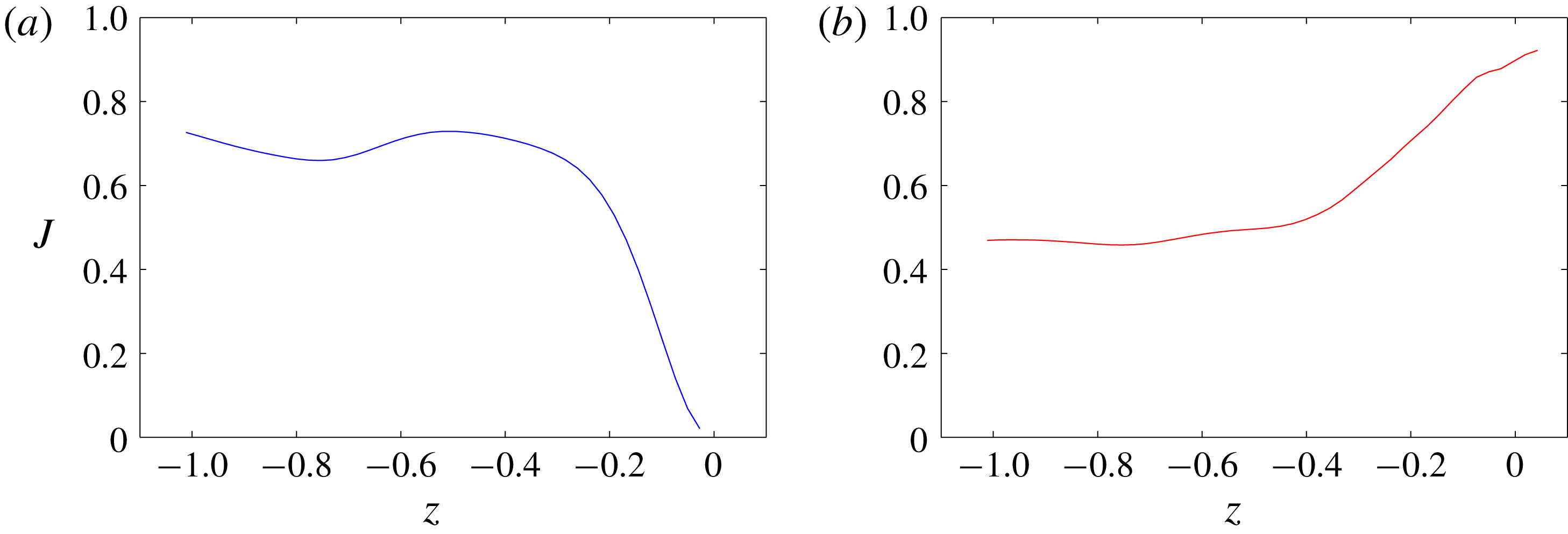
Figure 13(a) presents the turbulent isotropy parameter
 $J$
as a function of
 $z$
.
 $J$
is defined by:
 $$\begin{eqnarray}J=1-9\left({\textstyle \frac{1}{2}}\unicode[STIX]{x1D623}_{ij}\unicode[STIX]{x1D623}_{ij}-\unicode[STIX]{x1D623}_{ij}b_{jk}b_{ki}\right).\end{eqnarray}$$
Here,
 $J$
is bounded
 $J\in [0,1]$
, where
 $J=1$
is fully isotopic. In the WFST case, the value of
 $J$
drops sharply as
 $z$
approaches 0, indicating turbulence near the free surface is highly anisotropic. For SFST, however,
 $J$
approaches a value of 0.92 at the free surface, suggesting nearly isotropic turbulence.
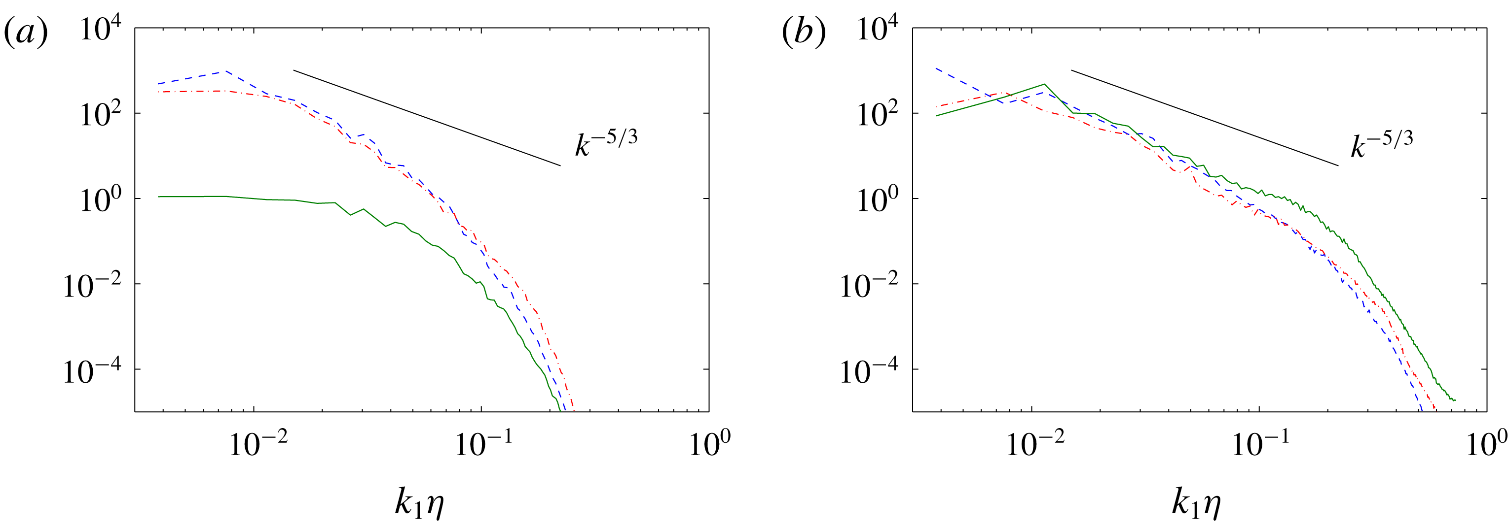
Finally, we confirm this anisotropic behaviour using the three one-dimensional energy spectra (calculated from velocity fluctuations) at
 $z=0$
as shown in figure 14. In WFST, the suppression of the vertical component is evident by the two orders of magnitude difference in the energy compared to the two horizontal components. In SFST, all three components have comparable magnitudes and follow the Kolmogorov spectra
 $k^{-5/3}$
of isotropic turbulence. Because of the isotropy of turbulence in the flow with anisotropic mean strain rate, turbulent closure models of the Boussinesq type, which approximate the Reynolds stress using the mean strain rate, are likely not appropriate for sheared SFST.
The Lumley triangle on the plane of the invariants
 $\unicode[STIX]{x1D709}$
and
 $\unicode[STIX]{x1D702}$
of the anisotropy tensor from the bulk flow
 $z=-1$
to the free surface
 $z=0$
at
 $t=90$
. ▫, SFST;
 $\circ$
, WFST.

Turbulent isotropy parameter
 $J$
as a function of
 $z$
(a) WFST; (b) SFST.

One-dimensional energy spectra
 $E_{11}(k_{1})$
(– – –),
 $E_{22}(k_{1})$
(— ⋅ —),
 $E_{33}(k_{1})$
(——) near the free surface at
 $t=90$
in (a) WFST with
 $Fr^{2}=0.5$
and
 $We=\infty$
; (b) SFST with
 $Fr^{2}=10$
and
 $We=\infty$
.

5 Air entrainment and bubble size distribution in SFST
Brocchini & Peregrine (Reference Brocchini and Peregrine2001a
) proposed a conceptual map in the
 $(l,q)$
-plane for FST flows. In the SFST case of
 $Fr^{2}=10$
and
 $We=\infty$
, for physical length and velocity scales of
 $L=1~\text{m}$
and
 $U=1~\text{m}~\text{s}^{-1}$
, say, the turbulent velocity
 $q$
would be approximately
 $0.12~\text{m}~\text{s}^{-1}$
and the length scale of cavities
 $l$
would be in the range between 0.01 m and 0.1 m. The current SFST would thus be located in the strong turbulence regime (or region 2 of Brocchini & Peregrine Reference Brocchini and Peregrine2001a
) of the
 $(l,q)$
-plane. In this regime, turbulence is sufficiently strong that neither gravity nor surface tension can maintain surface cohesion, and air entrainment is expected to happen. These descriptions are consistent with our observations. We define
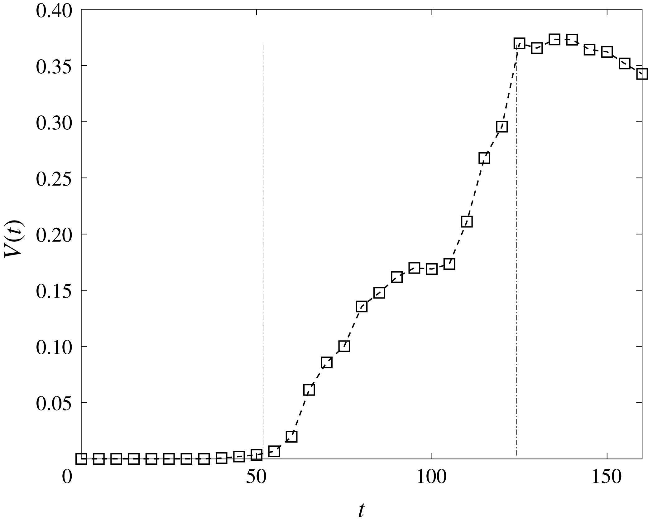
 $V(t)$
as the total volume of air entrainment in the computational domain. Figure 15 presents the evolution of
 $V(t)$
for the SFST case with (large)
 $Fr^{2}=10$
and
 $We=\infty$
. Air entrainment occurs after
 $t_{s}\approx 55$
and
 $V(t)$
continues to increase until
 $t_{e}\approx 125$
, beyond which air entrainment ceases and
 $V(t)$
begins to decrease due to degassing. Strictly speaking,
 $V(t)$
is affected by concurrent air degassing throughout the entrainment period
 $t_{s}\leqslant t\leqslant t_{e}$
(with duration
 $T_{a}$
), although for this problem, the degassing rate is small compared to air entrainment (which will be confirmed later). For specificity and later use, we define the air entrainment rate
 $Q=\dot{V}(t)$
, and quantify an average air entrainment rate (or average air flux)
 $\overline{Q}_{V}=(1/T_{a})V(t_{e})$
as the average of
 $Q$
over the entrainment period, which approximately overlaps with the quasi-steady duration of TKE, see figure 6. From figure 15, we estimate
 $\overline{Q}_{V}\approx 0.006$
for the current SFST case.
Evolution of total volume of air entrainment
 $V(t)$
for SFST of
 $Fr^{2}=10$
and
 $We=\infty$
. – – – marks the entrainment period.

Bubble size spectrum
 $N_{a}(r)$
as a function of
 $r$
for SFST of
 $Fr^{2}=10$
and
 $We=\infty$
in the entrainment period:
 $t=60$
(
 $\circ$
),
 $t=70$
(▫) and
 $t=120$
(▿). ——
 $r^{-10/3}$
and – – –:
 $r^{-6}$
. Inset:
 $N_{a}(r)$
in the post-entrainment period:
 $t=135$
(
 $\ast$
) and
 $t=160$
(
 $+$
).

To quantitatively describe the bubble size distribution of entrainment across the free surface in SFST, the key is to model the number of bubbles of a particular radius
 $r$
entrained through a given (initial flat or mean) area of the free surface. For this purpose, we introduce the quantity
 ${\mathcal{N}}_{a}^{E}(r)$
, where
 ${\mathcal{N}}_{a}^{E}(r)\,\text{d}r$
is the number of bubbles of radius between
 $r$
and
 $r+\text{d}r$
entrained per unit area of the mean free surface. The dimension of
 ${\mathcal{N}}_{a}^{E}(r)$
is then
 $L^{-3}$
. Here, we provide an energy scaling argument to obtain
 ${\mathcal{N}}_{a}^{E}(r)$
. The result depends on the (near-surface) turbulence energy spectrum of the SFST. As we pointed out in § 4, the present SFST is near isotropic under the surface with a Kolmogorov spectrum of
 $k^{-5/3}$
(see figure 14). For clarity, in this derivation, we revert to dimensional variables with physical units.
Assuming negligible surface tension, the minimum energy (potential energy) required to generate a bubble of radius
 $r$
just below the free surface (without considering its overall motion) (Brocchini & Peregrine Reference Brocchini and Peregrine2001a
) is,
 $$\begin{eqnarray}E_{b}(r)\sim gr^{3}r.\end{eqnarray}$$
Given the definition of
 ${\mathcal{N}}_{a}^{E}(r)$
and a (mean) free-surface area
 $A$
of interest, the total energy required to entrain all bubbles of radius
 $r$
 $$\begin{eqnarray}E_{e}(r)\sim {\mathcal{N}}_{a}^{E}(r)A\,\text{d}r\,E_{b}(r).\end{eqnarray}$$
According to Brocchini & Peregrine (Reference Brocchini and Peregrine2001a
), this amount of energy is supplied by turbulence surrounding the entrained bubbles. In the specific entrainment scenario considered in (5.1) where a bubble is formed right below the free surface, for the free surface of (mean) area
 $A$
considered here, all the bubbles of radius between
 $r$
and
 $r+\text{d}r$
(of number
 ${\mathcal{N}}_{a}^{E}(r)A\,\text{d}r$
) are considered to be primarily formed in a volume
 $Ar$
under the free surface. Therefore, the total amount of energy
 $E_{e}(r)$
for entraining bubbles of radius
 $r$
comes from near-surface turbulence over this volume. If
 $\unicode[STIX]{x1D700}(k)$
is the turbulence energy spectrum, the energy of turbulence at length scale
 $1/k$
is
 $|\unicode[STIX]{x1D700}(k)\,\text{d}k|$
. If we consider turbulence energy of length scale comparable to
 $r$
, the total amount of available turbulence energy in the volume
 $Ar$
for entrainment of bubbles of radius
 $r\sim k^{-1}$
is
 $$\begin{eqnarray}E_{t}(r)\sim |\unicode[STIX]{x1D700}(k)\,\text{d}k|Ar=\unicode[STIX]{x1D700}(r^{-1})r^{-1}A\,\text{d}r.\end{eqnarray}$$
From § 4, we observe that the near-surface turbulence in SFST is approximately isotropic, so that we may assume a Kolmogorov spectrum
 $\unicode[STIX]{x1D700}(r^{-1})\propto \unicode[STIX]{x1D716}^{2/3}r^{5/3}$
for (5.3). Connecting (5.1) and (5.3), we finally obtain
 $$\begin{eqnarray}{\mathcal{N}}_{a}^{E}(r)\sim g^{-1}\unicode[STIX]{x1D716}^{2/3}r^{-10/3}.\end{eqnarray}$$
Several remarks are in order. First, the scaling
 ${\mathcal{N}}_{a}^{E}(r)\propto r^{-10/3}$
for surface air entrainment from (5.4) is the same as the one obtained by Garrett et al. (Reference Garrett, Li and Farmer2000). However, the underlying physical processes considered in these two models are different. In the model of Garrett et al. (Reference Garrett, Li and Farmer2000), a constant source of air is entrained at a given (large) scale which cascades and creates small bubbles, through bubble fragmentation, into a quasi-steady distribution following a
 $-10/3$
power law. Our model considers the entrainment process driven by near-surface turbulence. In particular, equation (5.4) is a result of near-surface isotropic SFST turbulence spectrum, and the power-law slope
 ${\mathcal{N}}_{a}^{E}(r)\propto r^{-10/3}$
would be modified accordingly if a different near-surface energy spectrum were obtained. Second, the surface entrainment model (5.4) only considers the process of entrainment, but not the subsequent bubble fragmentation and degassing in the volume. However, the bubble size spectrum measured in the bulk,
 $N_{a}(r)$
, is under the influence of all the three physical processes. Thus, the scale dependence of
 $N_{a}(r)$
may evolve over time and become distinguished from
 ${\mathcal{N}}_{a}^{E}(r)$
. In the current SFST, the degassing process is negligible on comparing the degassing rate to the entrainment rate. Still, we point out that the combined ongoing surface entrainment (over a size spectrum) and bulk fragmentation processes would not, in general, result in a constant bulk bubble size spectrum given by
 $r^{-10/3}$
. We will later provide a heuristic model to understand the effect of bubble fragmentation on
 $N_{a}(r)$
. Finally, the model in (5.4) predicts that the magnitude of
 ${\mathcal{N}}_{a}^{E}(r)$
scales as
 $g^{-1}$
and
 $\unicode[STIX]{x1D716}^{2/3}$
. These two scale dependencies need to be further tested to demonstrate the validity of (5.4). In § 6.1, we will present results showing that the averaged entrainment rate and the averaged increase rate of
 $N_{a}(r)$
magnitude indeed show a linear dependence on
 $g^{-1}$
. These results support the model prediction on
 $g^{-1}$
dependence in (5.4).
In the initial phase of SFST air entrainment,
 $t\gtrsim t_{a}$
, before significant bubble fragmentation has occurred, we argue that
 $N_{a}(r)$
should approximately follow (5.4). As the (quasi-steady) SFST air entrainment continues, the evolution of
 $N_{a}(r)$
depends on two ongoing processes: (i) the surface entrainment over a scale given by (5.4); and (ii) the subsequent fragmentation cascade of all the entrained bubbles up to this point. The combined process is complex and it is not clear whether a power-law distribution would be obtained (or if so, what the slope might be). For cVOF, we are able to quantify the bubbles in the bulk with time and obtain the corresponding bubble size spectrum
 $N_{a}(r)$
, but not directly the air entrainment, which is inferred from the bulk statistics. Thus it is difficult to separate the entrainment from the fragmentation effects in the bubble size spectra. Figure 16 shows
 $N_{a}(r)$
obtained from DNS at different instances of time within the quasi-steady entrainment period
 $55\lesssim t\lesssim 125$
, for the SFST case with
 $Fr^{2}=10$
and
 $We=\infty$
. At a relatively early instant after initiation of entrainment,
 $t=60$
,
 $N_{a}(r)$
indeed follows closely the
 ${\sim}r^{-10/3}$
power law of (5.4). As
 $t$
increases, the overall magnitude of
 $N_{a}(r)$
increases as new air is entrained into the water volume. However,
 $N_{a}(r)$
is seen to deviate from the initial
 $-10/3$
power law, with the value of
 $N_{a}(r)$
at small
 $r$
increasing faster than that at large
 $r$
.
To provide some qualitative insight into this evolution, we suggest a heuristic model which combines the two main mechanisms of ongoing SFST entrainment and subsequent fragmentation cascades of these bubbles. For the ongoing entrainment process, bubbles are considered to be entrained instantaneously over a broad range of scales given by (5.4) (only) at one instant. For the bubble fragmentation process, we consider a canonical problem of the fragmentation of an initial population of bubbles following a size spectrum of (5.4) in turbulence (see appendix C). For the underlying turbulence field, we use an isotropic homogeneous turbulence (IHT) field to approximate the isotropic near-surface turbulence in the SFST. For simplicity, the evolving size spectrum is approximated by a power law with time-dependent slope given by:
 $$\begin{eqnarray}N_{0}(r,\unicode[STIX]{x1D70F})=r^{-(a\unicode[STIX]{x1D70F}+\unicode[STIX]{x1D6FD}_{0})}V_{0}^{-1},\end{eqnarray}$$
where
 $\unicode[STIX]{x1D70F}$
is the evolution time,
 $\unicode[STIX]{x1D6FD}_{0}=-10/3$
is prescribed, and
 $V_{0}$
is a normalization factor so that the integrated volume of (5.5) is 1 . From appendix C, we find
 $a\approx 0.24$
. Finally, we assume that
 $N_{a}(r,t)$
in SFST is a convolution of (5.5)
 $$\begin{eqnarray}N_{a}(r,t)=\int _{t_{s}}^{t}\,\text{d}t_{0}\,Q(t_{0})N_{0}(r,t-t_{0}),\quad t>t_{s},\end{eqnarray}$$
where
 $Q(t_{0})$
is the volume entrainment rate at
 $t=t_{0}$
.
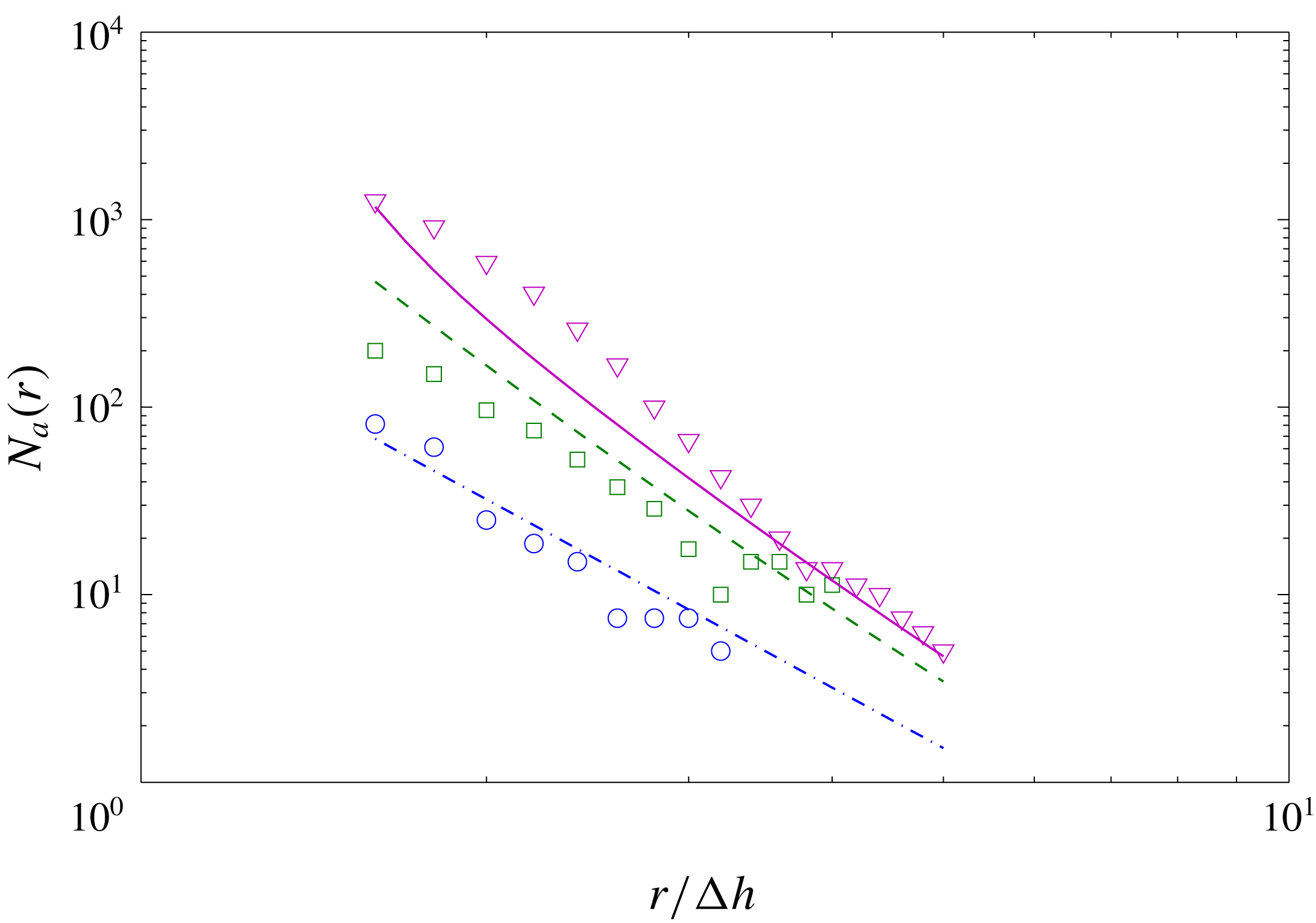
The usefulness of the heuristic model must be checked against DNS prediction. Figure 17 shows the comparison of (5.6) using the
 $Q(t)$
from DNS. Despite the simplicity of (5.6) and the substantial approximations involved, especially (5.5), the qualitative correspondence between (5.6) and DNS data suggests that the underlying processes represented in (5.6) are likely responsible for the evolution of
 $N_{a}(r)$
in figure 16.
Comparison of
 $N_{a}(r)$
at different time instances between equation (5.6) and DNS results of SFST with
 $Fr^{2}=10$
and
 $We=\infty$
. DNS (
 $\circ$
) and model prediction (— - —) at
 $t=60$
; DNS (▫) and model prediction (– – –) at
 $t=70$
; and DNS (▿) and model predictions (——) at
 $t=120$
.

Referring to figure 15,
 $t\geqslant 125$
marks the beginning of the post entrainment period. During this period (between 125 and 160), the near-surface turbulence intensity continues to decay (cf. figure 6), leading to the stop of the entrainment process. The decrease in
 $V(t)$
in figure 15 is a result of degassing (recall that cVOF conserves volume to machine accuracy). Analogous to the average entrainment rate
 $\overline{Q}_{V}$
, we estimate the average degassing rate over the post entrainment period
 $\overline{Q}_{d}=(V(t=125)-V(t=160))/(160-125)\approx 0.0006$
. We see that
 $\overline{Q}_{d}$
is an order of magnitude smaller than
 $\overline{Q}_{V}$
(which is
 ${\approx}0.006$
). This supports our earlier assumption that degassing is relatively unimportant during the entrainment period. Further evidence of the degassing process is seen in figure 16(inset) where the number of large bubbles decreases faster than the number of small bubbles for
 $N_{a}(r)$
at
 $t=135$
and
 $t=160$
. This indicates that larger bubbles are escaping the water volume faster due to buoyancy effects. Further elucidation of the general degassing processes would benefit from Lagrangian tracking, which is difficult in the context of VOF (in the presence of ongoing turbulent entrainment, fragmentation, coalescence and advection), and is beyond the scope of the present work.
Analogous to
 $\overline{Q}_{V}$
for the average entrainment rate, we define for later reference the average rate of increase of the bubble spectrum
 $\overline{Q}_{N}(r)=(1/T_{a})N_{a}(r,t=t_{e})$
(averaged over the same entrainment period as
 $\overline{Q}_{V}$
).
6 The effects of
$Fr$
and
$We$
on air entrainment


In FST flows, air entrainment is a consequence of two competing effects on the free surface. One is the disrupting effect of near-surface turbulence, which deforms the free surface and entrains air. The other is the stabilization effect due to gravity and surface tension, both of which stabilize the free surface and prevent air entrainment. Therefore, the two main parameters controlling air entrainment in FST are
 $Fr$
and
 $We$
. In general, the air entrainment volume is affected by both
 $Fr$
and
 $We$
. To elucidate the underlying physics, in this work, we focus on the dependence of air entrainment on each of the two parameters independently by varying
 $Fr$
for some sufficiently large
 $We$
where surface tension effects are small; and varying
 $We$
for a (relatively large) fixed value of
 $Fr$
where gravity effects become small. For quantitative practical interest, it is would in general be necessary to cover a more significant portion of the
 $Fr$
–
 $We$
parameter space. This is beyond the scope of this work.
6.1 Dependence of air entrainment on
$Fr$

Time evolution of total entrainment volume
 $V(t)$
at different
 $Fr$
with
 $We=\infty$
(
 $\ast$
,
 $Fr^{2}=3$
;
 $\circ$
,
 $Fr^{2}=8$
; ▫,
 $Fr^{2}=10$
;
 $\diamondsuit$
,
 $Fr^{2}=12$
; ▵,
 $Fr^{2}=14$
).

Average entrainment rate
 $\overline{Q}_{V}$
as a function of
 $Fr^{2}$
with
 $We=\infty$
. —— linear fit.

(a) Bubble size spectrum
 $N_{a}(r)$
at the end of the entrainment period
 $t=125$
and (b) average rate of increase of bubble spectrum
 $\overline{Q}_{N}(r)$
of different
 $Fr$
with
 $We=\infty$
(
 $\circ$
,
 $Fr^{2}=8$
; ▫,
 $Fr^{2}=10$
;
 $\diamondsuit$
,
 $Fr^{2}=12$
; ▵,
 $Fr^{2}=14$
).

Time evolution of (a) turbulent kinetic energy near the free surface
 $\frac{1}{2}\langle q^{2}\rangle _{\unicode[STIX]{x1D6FF}}$
and (b) turbulent dissipation near the free surface
 $\langle \unicode[STIX]{x1D716}\rangle _{\unicode[STIX]{x1D6FF}}$
at different
 $Fr$
with
 $We=\infty$
. (
 $\circ$
,
 $Fr^{2}=8$
; ▫,
 $Fr^{2}=10$
;
 $\diamondsuit$
,
 $Fr^{2}=12$
; ▵,
 $Fr^{2}=14$
).

To investigate the effect of
 $Fr$
on air entrainment, we vary
 $Fr$
(
 $Fr^{2}=3,8,10,12$
and
 $14$
) while maintaining negligible surface tension by choosing
 $We=\infty$
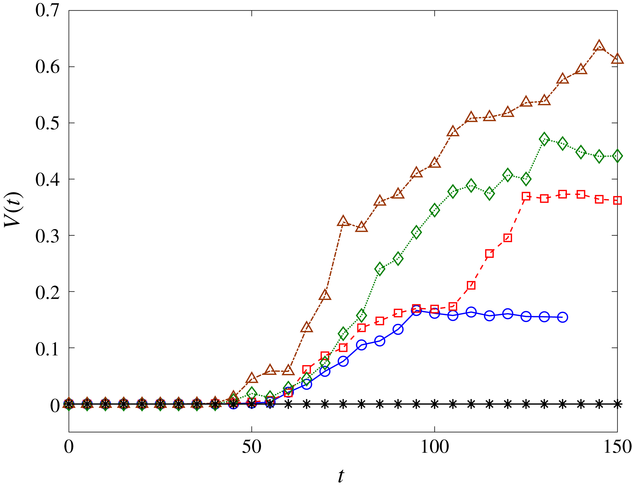
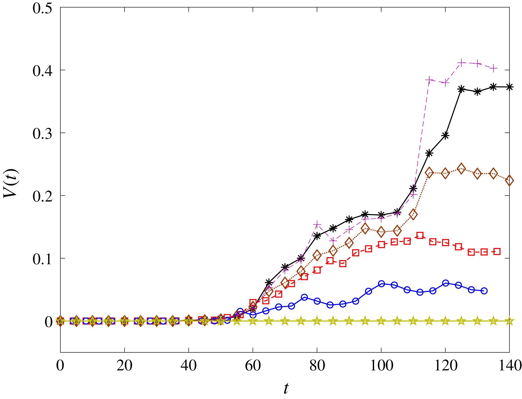
. Figure 18 shows the time evolution of the total entrainment volume
 $V(t)$
for a range of
 $Fr$
. From these results, we find a critical
 $Fr_{cr}$
below which no air is entrained. For this particular flow with
 $We=\infty$
,
 $Fr_{cr}^{2}\approx 5$
. Figure 18 shows a clear relationship between
 $V(t)$
and
 $Fr$
for
 $Fr>Fr_{cr}$
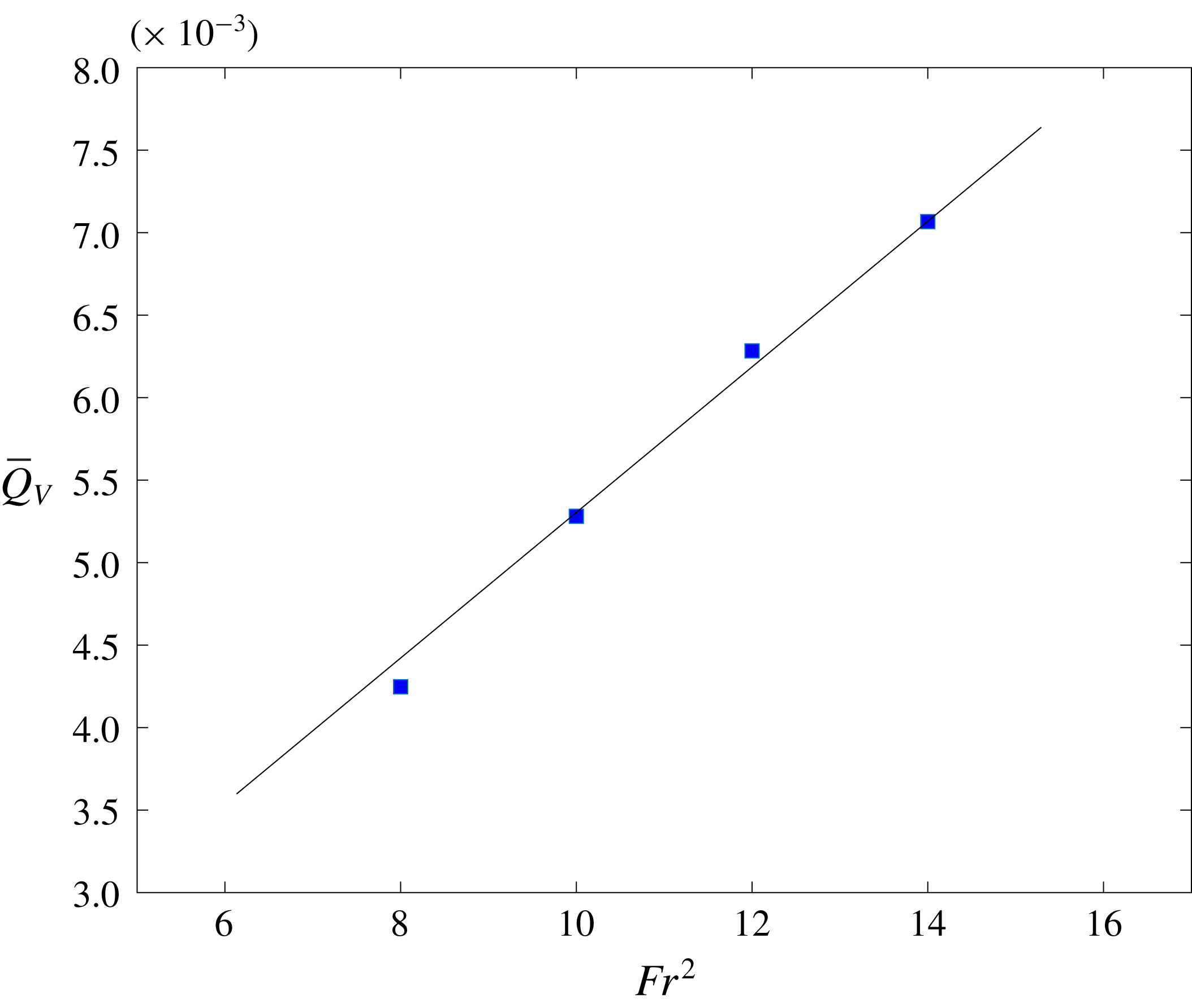
. Figure 19 shows the average entrainment rate
 $\overline{Q}_{V}$
as a function of
 $Fr^{2}$
(with
 $We=\infty$
), establishing a linear dependence of
 $\overline{Q}_{V}$
on
 $Fr^{2}$
(or
 $g^{-1}$
).
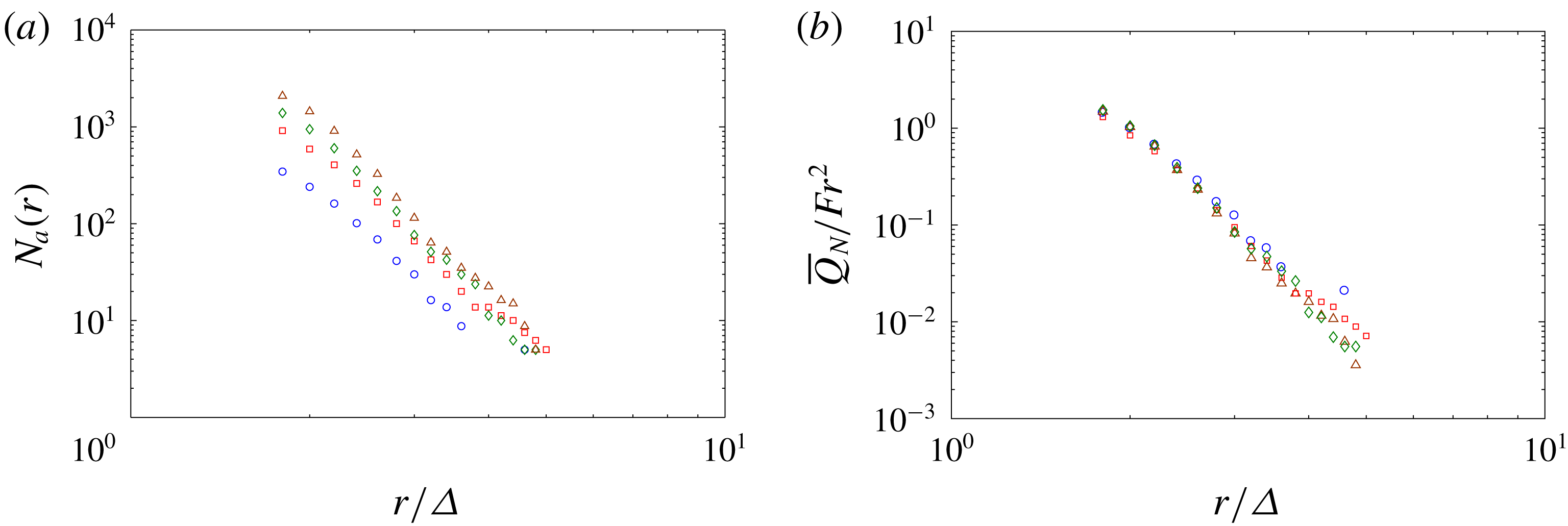
Figure 20 shows the bubble size spectrum
 $N_{a}(r)$
for the varying
 $Fr$
cases at the end of the entrainment period. The results in figure 20(a) suggest an increase in the overall number of entrained bubbles with increasing
 $Fr$
. Figure 20(b) shows the average rate of increase of bubble spectrum scaled by
 $Fr^{2}$
,
 $\overline{Q}_{N}(r)/Fr^{2}$
, resulting in a collapse of the data. This further confirms the linear dependence of air entrainment rate on
 $Fr^{2}$
.
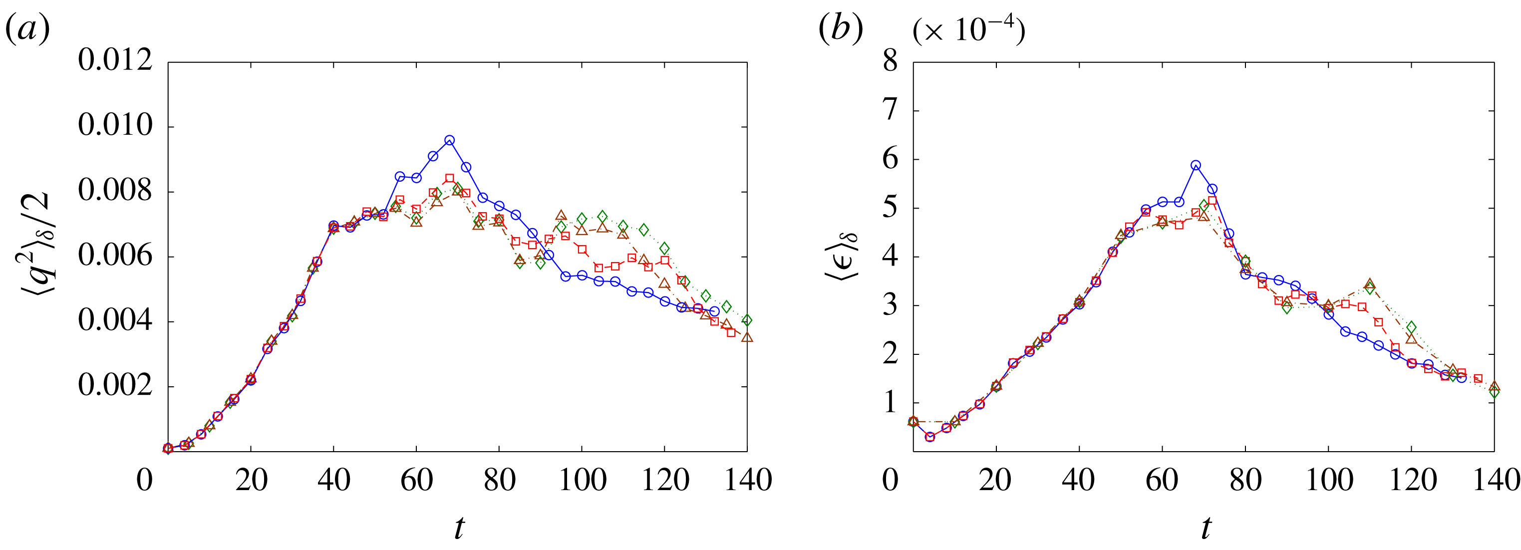
The four
 $Fr$
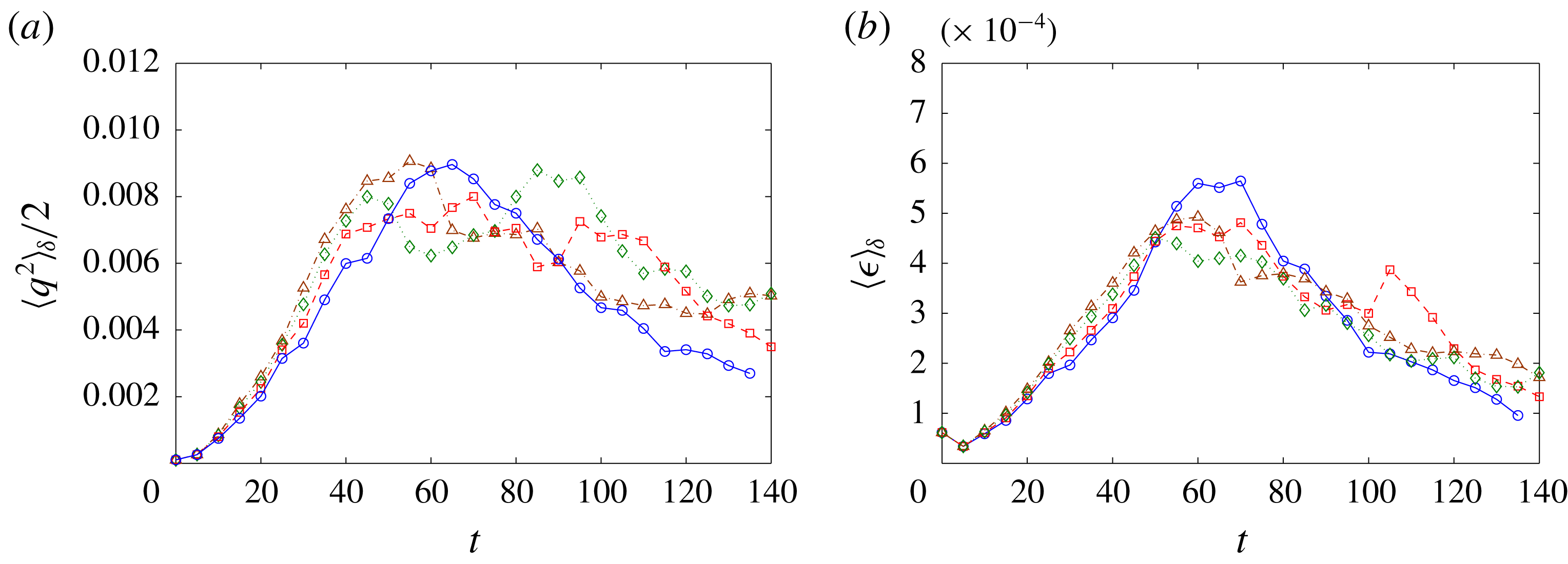
considered in figure 18 fall within the strong turbulence regime and their basic features are the same as discussed in § 4. Figure 21 shows the evolution of the near-surface turbulent kinetic energy
 $\frac{1}{2}\langle q^{2}\rangle _{\unicode[STIX]{x1D6FF}}$
(figure 21
a) and turbulent dissipation rate
 $\langle \unicode[STIX]{x1D716}\rangle _{\unicode[STIX]{x1D6FF}}$
(figure 21
b). Here,
 $\langle \unicode[STIX]{x1D716}\rangle _{\unicode[STIX]{x1D6FF}}$
is defined as
 $1/Re\langle (\unicode[STIX]{x2202}u_{i}/\unicode[STIX]{x2202}x_{k})(\unicode[STIX]{x2202}u_{i}/\unicode[STIX]{x2202}x_{k})\rangle _{\unicode[STIX]{x1D6FF}}$
. Despite the sizeable variation of
 $Fr$
, the effect of
 $Fr$
on the available near-surface turbulence energy is limited. Thus the observed dependence of
 $\overline{Q}_{V}$
on
 $Fr^{2}$
is primarily a result of the change of the gravity effects on the air–water interface (through the stabilization on the free surface).
6.2 Dependence of air entrainment on
$We$

Time evolution of total entrainment volume
 $V(t)$
at different
 $We$
with
 $Fr^{2}=10$
(
 $\star$
,
 $We=100$
;
 $\circ$
,
 $We=1000$
; ▫,
 $We=4000$
;
 $\diamondsuit$
,
 $We=10\,000$
;
 $+$
,
 $We=50\,000$
;
 $\ast$
,
 $We=\infty$
).

Average entrainment rate
 $\overline{Q}_{V}$
as a function of
 $We$
with
 $Fr^{2}=10$
. —— linear fit.

To investigate the effect of
 $We$
on air entrainment, we vary
 $We$
(
 $We=100$
,
 $1000$
,
 $4000$
,
 $10\,000$
,
 $15\,000$
and
 $50\,000$
) while maintaining
 $Fr^{2}=10$
. Our interest here is for FST with sufficiently large
 $Fr$
(
 $Fr^{2}=O(10)$
) where SFST and air entrainment occur. Figure 22 shows the time evolution of the total entrainment volume
 $V(t)$
for a range of
 $We$
. From these results, we also find a critical
 $We_{cr}$
, below which air entrainment is suppressed. For this particular flow with
 $Fr^{2}=10$
,
 $We_{cr}$
is found to be of
 $O$
(100). Figure 22 shows a clear relationship between
 $V(t)$
and
 $We$
for
 $We>We_{cr}$
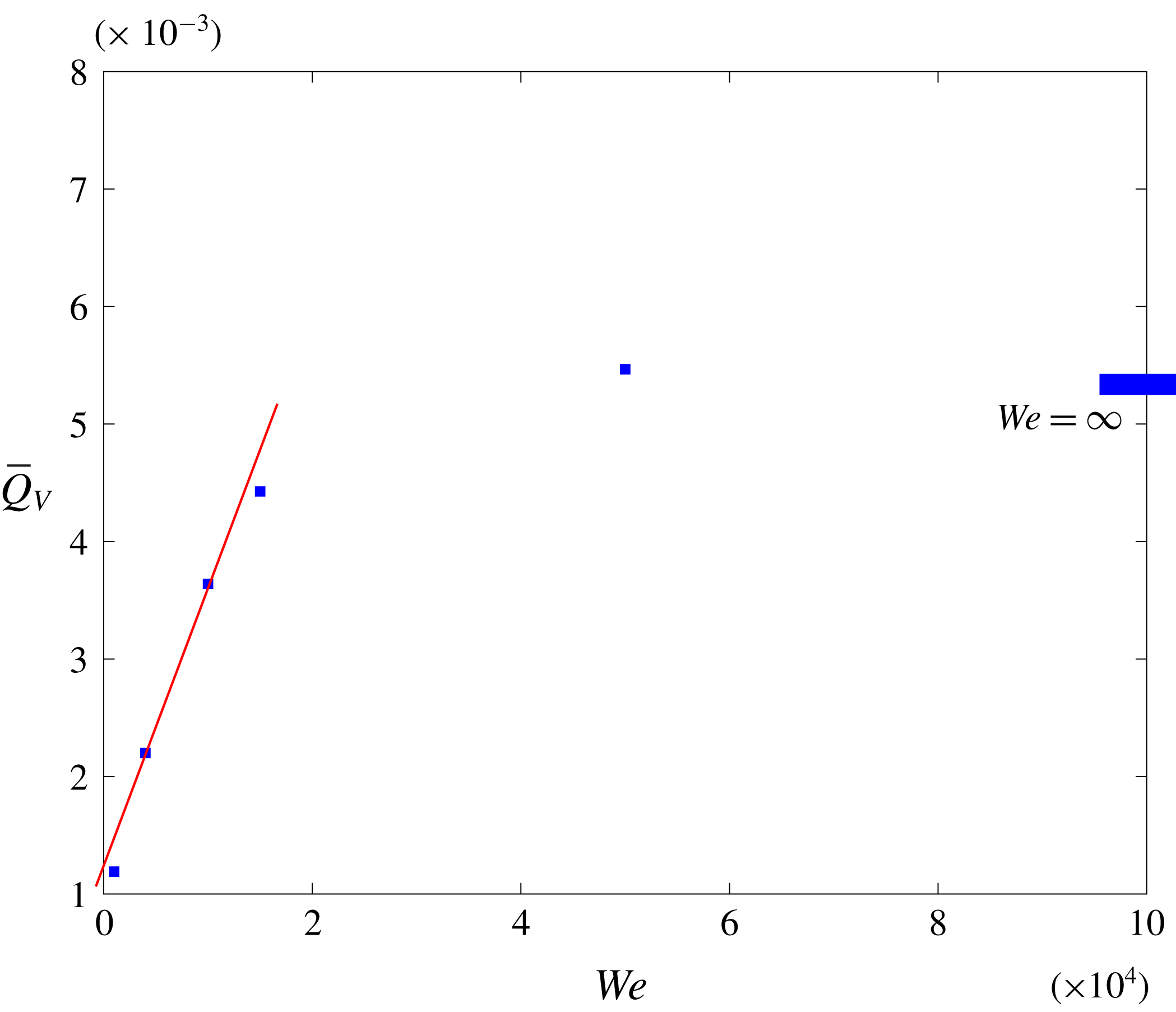
. Figure 23 shows the average entrainment rate
 $\overline{Q}_{V}$
as a function of
 $We$
with given
 $Fr^{2}=10$
. In figure 23, the dependence of
 $\overline{Q}_{V}$
on
 $We$
shows two regimes. For
 $We\gtrsim O(W_{e1})=O(3\times 10^{4})$
,
 $\overline{Q}_{V}$
converges to the value of the case with
 $We=\infty$
. For
 $We\lesssim O(W_{e1})$
,
 $\overline{Q}_{V}$
is observed to be linearly dependent on
 $We$
. We argue that the two regimes correspond to important or unimportant surface tension relative to gravity, delineated by
 $Bo_{r}=\unicode[STIX]{x1D70C}gl_{c}^{2}/\unicode[STIX]{x1D70E}\approx 1$
with the capillary length scale
 $l_{c}$
being a characteristic length scale of a bubble size of order
 $\unicode[STIX]{x1D6E5}$
. For
 $We\gtrsim O(W_{e1})$
,
 $l_{c}$
is
 ${\lesssim}\unicode[STIX]{x1D6E5}$
and the effects of surface tension on scales we resolve in DNS are negligible relative to gravity. In figure 23,
 $\overline{Q}_{V}$
at
 $We=5\times 10^{4}$
is observed to be close to the value at
 $We=\infty$
. Therefore, rather than fixing some
 $We>O(W_{e1})$
, we can use
 $We=\infty$
to approximate the cases where surface tension effects are negligible (and
 $Fr$
is the controlling parameter for bubble entrainment). For
 $We\lesssim O(W_{e1})$
,
 $l_{c}$
is comparable to the entrainment scales we resolve and surface tension becomes important on air entrainment. For the four cases with
 $We=1000,4000,10\,000,15\,000$
in figure 23,
 $l_{c}$
is resolved by at least one grid cell. For the case of
 $We=1000$
with strongest surface tension of all the cases,
 $l_{c}$
is resolved by four grid cells. The corresponding
 $\overline{Q}_{V}$
is observed to be linearly dependent on
 $We$
(or
 $(\unicode[STIX]{x1D70E}/\unicode[STIX]{x1D70C})^{-1}$
).
Another relevant parameter for bubble entrainment is
 $We_{T}=\unicode[STIX]{x1D70C}\langle q^{2}\rangle _{\unicode[STIX]{x1D6FF}}\ell _{t}/\unicode[STIX]{x1D70E}$
, where
 $\langle q^{2}\rangle _{\unicode[STIX]{x1D6FF}}$
represents the turbulent kinetic energy near the free surface (see figure 24
a). The length scale,
 $\ell _{t}=(\langle q^{2}\rangle _{\unicode[STIX]{x1D6FF}}We)^{-1}$
for
 $We_{T}=1$
, represents the scale of capillary surface deformation introduced by turbulence. To simulate the entrainment under strong surface tension, we need to have
 $\ell _{t}$
resolved or
 $\ell _{t}\gtrsim O(\unicode[STIX]{x1D6E5})$
. Equivalently, we need
 $We\lesssim O(10^{4})$
. For the four cases with
 $We=1000,4000,10\,000,15\,000$
, the surface tension effects on the entrainment process are important and being properly resolved.
We point out that the transition of the two regimes observed in figure 23 corresponds to
 $Bo_{r}\sim 1$
instead of
 $We_{T}\sim 1$
, although in figure 23 both happen to be close to
 $We\sim O(10^{4})$
. As pointed out earlier, air entrainment in FST is a consequence of the competition of the disrupting effect of near-surface turbulence and the stabilization effect from gravity and surface tension;
 $Bo_{r}$
represents the gravity effect compared to surface tension and
 $Bo_{r}\sim 1$
, thus, suggests the transition of dominance of surface tension or gravity. At
 $Bo_{r}\sim 1$
, the main stabilization force on the free surface is shifted from surface tension to gravity, which suggests a mechanism change of the stabilization force competing with turbulence disturbance. The convergence of
 $\overline{Q}_{V}$
after the transition in figure 23 is because the surface tension effects become negligible relative to the unchanged gravity effects (with a fixed
 $Fr$
). On the other hand,
 $We_{T}$
represents the disrupting effect of near-surface turbulence compared to the stabilizing effect of surface tension;
 $We_{T}\sim 1$
does not suggest significant changes in the underlying mechanisms.
For the
 $We\lesssim O(W_{e1})$
cases of interest,
 $\overline{Q}_{V}$
is believed to be accurate as
 $l_{c}$
and
 $\ell _{t}$
are resolved in our DNS. For
 $N_{a}(r)$
, however, the resolution of bubble shape (and surface tension forces) requires
 $r/\unicode[STIX]{x1D6E5}\gtrsim 4$
. Thus the bubble size range in
 $N_{a}(r)$
we resolve quantitatively in these cases is very limited by the present DNS resolution. Nevertheless,
 $N_{a}(r)$
plots similar to figure 20 (not shown) do indicate the same qualitative trends of power-law-like behaviours, with increasing
 $N_{a}$
amplitude that scales with
 $We$
. When scaled by
 $We$
,
 $\overline{Q}_{N}(r)/We$
for these cases also collapse into a single curve similar to figure 20(b).
The four flows are in the strong turbulence regime. Figure 24 shows the evolution of the turbulent kinetic energy
 $\frac{1}{2}\langle q^{2}\rangle _{\unicode[STIX]{x1D6FF}}$
and turbulent dissipation rate
 $\langle \unicode[STIX]{x1D716}\rangle _{\unicode[STIX]{x1D6FF}}$
in the near-surface region. Despite the sizeable variation of
 $We$
, the available energy of near-surface turbulence remains unaffected. Thus the observed dependence of
 $\overline{Q}_{V}$
on
 $We$
is primarily a result of the variation of surface tension on the air–water interface (through the stabilization on the free surface).
Time evolution of (a) turbulent kinetic energy near the free surface
 $\frac{1}{2}\langle q^{2}\rangle _{\unicode[STIX]{x1D6FF}}$
and (b) turbulent dissipation near the free surface
 $\langle \unicode[STIX]{x1D716}\rangle _{\unicode[STIX]{x1D6FF}}$
at different
 $We$
with
 $Fr^{2}=10$
. (
 $\circ$
,
 $We=1000$
; ▫,
 $We=4000$
;
 $\diamondsuit$
,
 $We=10\,000$
; ▵,
 $We=\infty$
.)

7 Conclusion
We perform DNS of a canonical three-dimensional two-phase (air and water) viscous turbulent flow with turbulent kinetic energy supplied by a sheared underlying water bulk flow. We investigate the characteristics of strong free-surface turbulence and air entrainment associated with large
 $Fr$
and
 $We$
. We elucidate the qualitatively distinct characteristics of strong versus weak free-surface turbulence. For WFST, the near-surface flow is characterized by the presence of the inner surface and outer blockage layers, resulting in strong anisotropy of the FST. Furthermore, free-surface displacements/disturbances are small and no air entrainment is observed. In contrast, for SFST, the free surface is strongly distorted by turbulence with significant displacements, distortions and, ultimately, breakup of the interface. In the underlying flow, the surface and blockage layers weaken and disappear, and the FST becomes almost isotropic. We document the latter by quantifying the anisotropy tensor
 $\unicode[STIX]{x1D623}_{ij}$
and an isotropic parameter
 $J$
of the SFST. We also find that the corresponding turbulence energy spectrum follows approximately the
 $k^{-5/3}$
Kolmogorov spectra of isotropic turbulence.
We use a cavity identification algorithm to quantify the air entrainment volume as well as the bubble size spectrum
 $N_{a}(r)$
of the entrained air in the bulk flow. With negligible surface tension,
 $N_{a}(r)$
is observed to follow a
 $r^{-10/3}$
power law at the early stage of the entrainment period, reflecting the size distribution of the surface entrainment. As the entrainment process continues, accompanied by the fragmentation of already entrained air,
 $N_{a}(r)$
deviates from the
 $-10/3$
power law. Using an energy argument for the scaling of the entrainment size distribution, and incorporating the evolution of the size spectrum of an initial population of bubbles into IHT, we provide a heuristic model that qualitatively matches and explains the salient evolution behaviour of
 $N_{a}(r)$
obtained from DNS.
We investigate the dependence of air entrainment on a broad range of
 $Fr$
and
 $We$
. We define an average entrainment volume rate
 $\overline{Q}_{V}$
(over a period when the air entraining SFST is quasi-static). We obtain the dependence of
 $\overline{Q}_{V}$
on
 $Fr$
and
 $We$
. When either
 $Fr^{2}$
or
 $We$
is below some respective critical values
 $Fr_{cr}^{2}$
and
 $We_{cr}$
,
 $\overline{Q}_{V}$
is small. For sufficiently large
 $We>We_{cr}$
and
 $Bo_{r}>O(1)$
,
 $\overline{Q}_{V}$
scales as
 $Fr^{2}$
for
 $Fr^{2}>Fr_{cr}^{2}$
. On the other hand, for sufficiently large
 $Fr^{2}>Fr_{cr}^{2}$
and
 $Bo_{r}<O(1)$
,
 $\overline{Q}_{V}$
scales as
 $We$
for
 $We>We_{cr}$
. These dependencies of
 $\overline{Q}_{V}$
on
 $Fr^{2}$
and
 $We$
are also supported by considering the corresponding average rate of increase of bubble spectrum
 $\overline{Q}_{N}(r)$
.
Acknowledgements
This work was funded by the Office of Naval Research N00014-10-1-0630 under the guidance of Dr K.-H. Kim and Dr T. C. Fu. The computational resources for the effort were funded through the High Performance Modernization Program at the Department of Defense.
Appendix A. Ensemble average and statistical error in the mean of DNS data
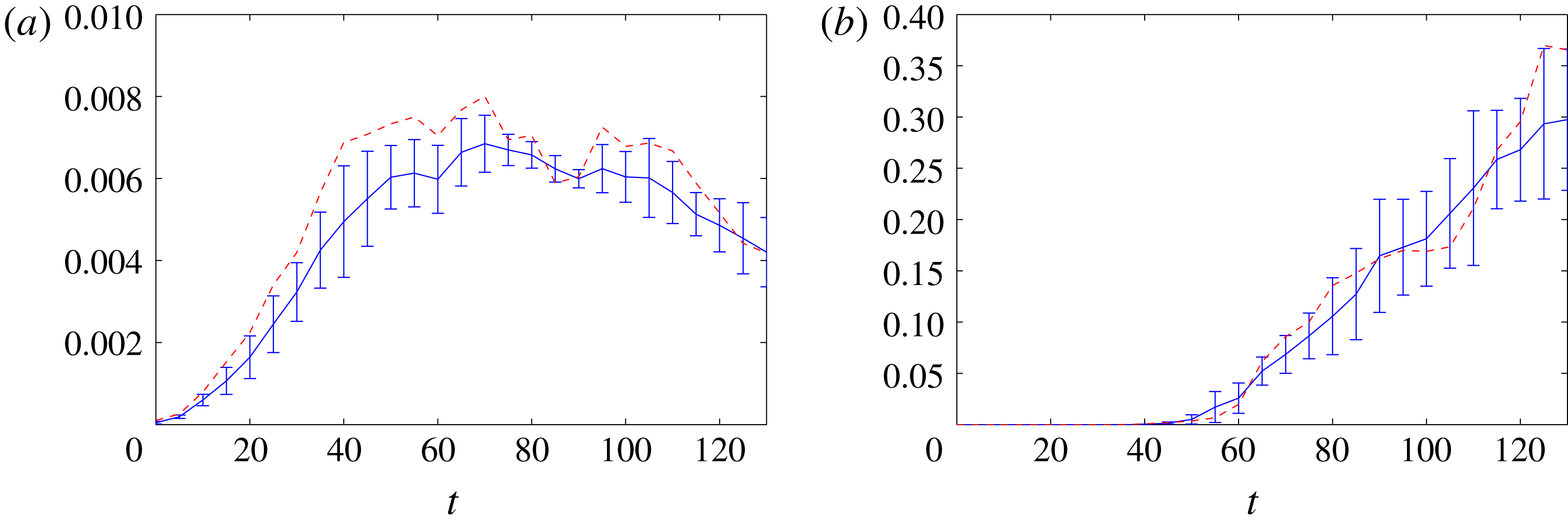
The data presented in §§ 4–6 represent a single realization with a particular initial perturbation. Statistical analysis (Morales, Nuevo & Rull Reference Morales, Nuevo and Rull1990) of the cases using this initial perturbation shows that the maximum error in the mean is less than 4 %. To establish the independence of the data from the initial perturbation, we perform 4 additional simulations of the SFST case with
 $Fr^{2}=10$
and
 $We=\infty$
. We find that all of the turbulence and air entrainment quantities show similar behaviour and statistics. For example, figure 25 shows the evolution of the turbulent kinetic energy
 $\frac{1}{2}\langle q^{2}\rangle _{\unicode[STIX]{x1D6FF}}$
and entrainment volume
 $V(t)$
, using ensemble averaging. The data used in §§ 4–6 are provided as a reference. The data from the single simulation are representative of the ensemble.
Evolution of (a) turbulent kinetic energy
 $\frac{1}{2}\langle q^{2}\rangle _{\unicode[STIX]{x1D6FF}}$
and (b) total entrainment volume
 $V(t)$
. —— ensemble average of 5 different initial perturbations with error bar identifying one standard deviation; – – – data from the single perturbation presented in §§ 4–6.

Appendix B. Definition of the near-surface region
We define the near-surface region as a thin layer of thickness
 $\unicode[STIX]{x1D6FF}$
below the free surface. We further define a turbulence quantity
 $q(\boldsymbol{x},t)$
near the free surface as a volume fraction weighted average
 $\langle q(t)\rangle _{\unicode[STIX]{x1D6FF}}$
over the whole layer,
 $$\begin{eqnarray}\langle q(t)\rangle _{\unicode[STIX]{x1D6FF}}=\frac{\displaystyle \int _{x}\int _{y}\int _{z}f(\boldsymbol{x},t)q(\boldsymbol{x},t)\,\text{d}\boldsymbol{x}}{\displaystyle \int _{x}\int _{y}\int _{z}f(\boldsymbol{x},t)\,\text{d}\boldsymbol{x}}\quad \text{for }z\geqslant -\unicode[STIX]{x1D6FF},\end{eqnarray}$$
where
 $f$
is the volume fraction. The choice of
 $\unicode[STIX]{x1D6FF}$
should be such to capture the effects of the free surface on the underlying turbulence. For WFST, the blockage layer thickness is
 $O$
(0.5) and the turbulence in this layer exhibits distinctly different characteristics than the bulk flow. Thus,
 $\unicode[STIX]{x1D6FF}\leqslant 0.5$
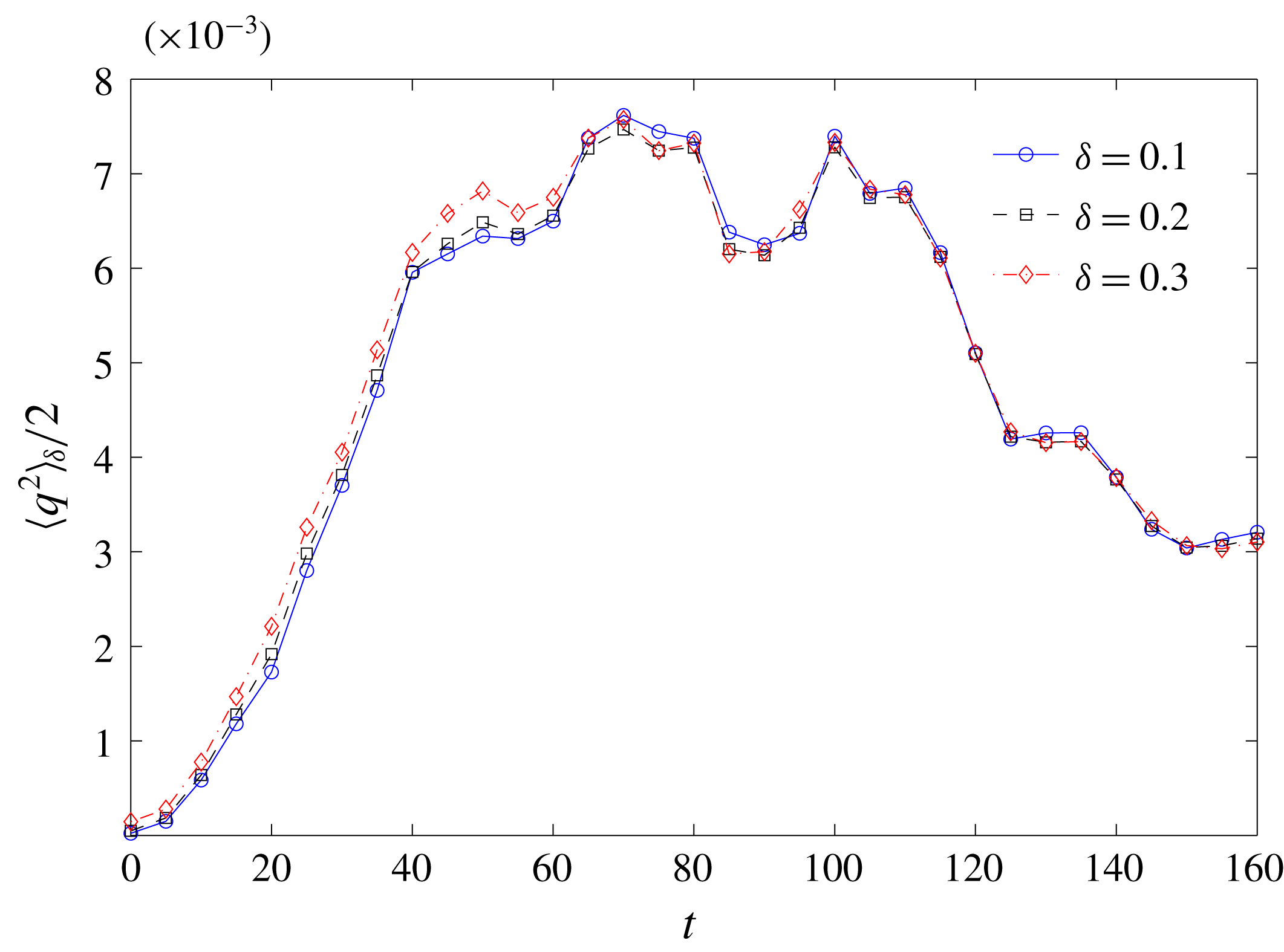
could be considered to be representative of ‘turbulence near the free surface’. Figure 26 shows the insensitivity of the turbulent kinetic energy in the near surface region to different
 $\unicode[STIX]{x1D6FF}$
. Thus, we choose
 $\unicode[STIX]{x1D6FF}=0.2$
to represent the thickness of the near free surface region and
 $\langle \cdot \rangle _{\unicode[STIX]{x1D6FF}}$
represents a volume-fraction-averaged quantity over the near free-surface region unless otherwise stated.
Time evolution of turbulent kinetic energy near the free surface
 $\frac{1}{2}\langle q^{2}\rangle _{\unicode[STIX]{x1D6FF}}$
using different values of
 $\unicode[STIX]{x1D6FF}$
of the flow
 $Fr^{2}=10$
and
 $We=\infty$
. - -
 $\circ$
- -
 $\unicode[STIX]{x1D6FF}=0.1$
; - -▫- -
 $\unicode[STIX]{x1D6FF}=0.2$
; and - -♢- -
 $\unicode[STIX]{x1D6FF}=0.3$
.

Appendix C. Bubble fragmentation in isotropic homogeneous turbulence
In this appendix, we consider the case of the fragmentation of a prescribed bubble field in isotropic homogenous turbulence (IHT). During the simulation, the method of linear forcing (Lundgren Reference Lundgren2003) is applied to IHT field to maintain the turbulent energy and prevent the decay of IHT. Initially, a one-phase DNS is simulated using white noise as an initial condition. The computational domain is a cube of length
 $3L$
, where
 $L$
is a length scale used for normalization. The domain is triply periodic with a resolution of
 $128^{3}$
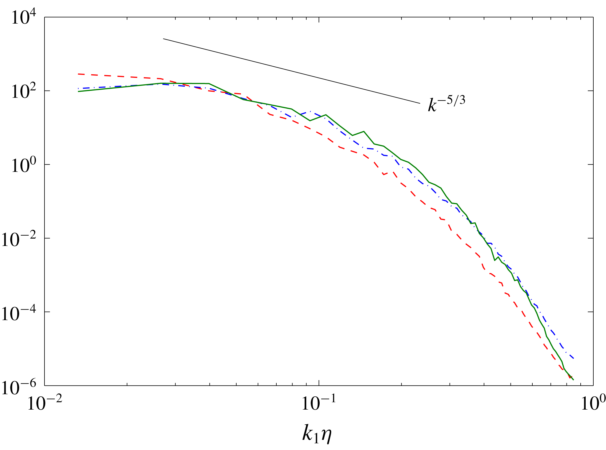
. As the flow evolves, the initial white noise field evolves to an IHT field. Figure 27 shows the one-dimensional energy spectrum
 $E_{ii}(k)$
of the developed IHT. The magnitude of
 $E_{11}$
,
 $E_{22}$
and
 $E_{33}$
plots are comparable with each other and follow the expected
 $k^{-5/3}$
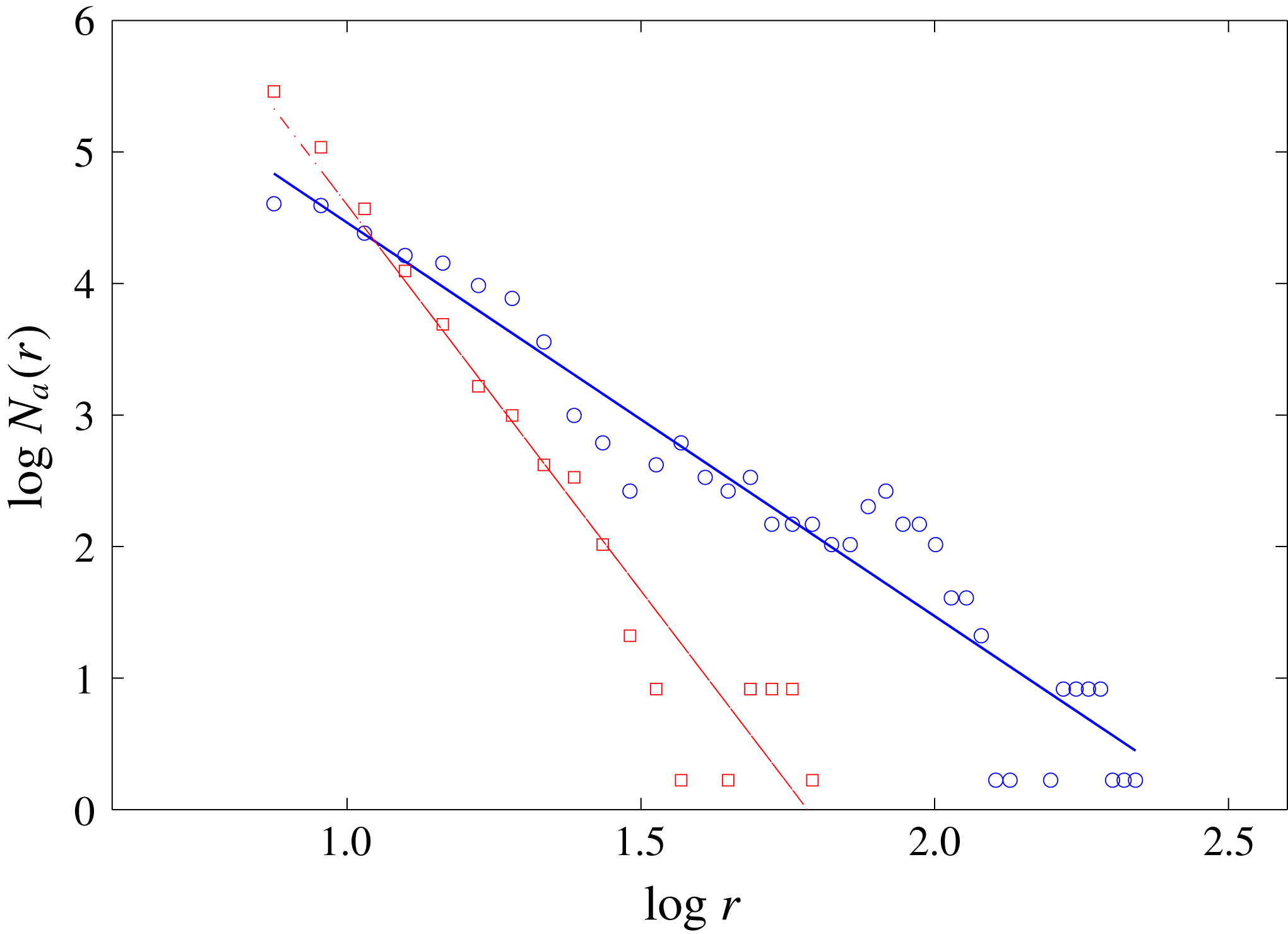
power law. Once the IHT is established, we introduce a bubble field in IHT. The initial bubble field consists of two hundred randomly placed bubbles sampled from a prescribed size spectrum of
 $N_{a}(r)\propto r^{-10/3}$
. The possible intersections of sampled bubbles are checked and avoided. The range of the bubble size is between 0.1
 $k\unicode[STIX]{x1D702}$
and 0.5
 $k\unicode[STIX]{x1D702}$
, corresponding to the horizontal axis in figure 27, which has an overlap with the inertial subrange of IHT. The bubbles are introduced with the velocity field intact so that the velocity field still satisfies continuity. In addition, the total void fraction of the bubbles is small, less than
 $1\,\%$
. Thus, the basic characteristics of the IHT field remain unaffected (Garrett et al.
Reference Garrett, Li and Farmer2000). The correct interfacial conditions are imposed by the cVOF method when the simulation starts. The Reynolds number, the range of bubble size, the total void fraction and turbulence intensity are chosen to match the SFST case. Gravity and surface tension effects are not included. Based upon a theoretical argument, bubble fragmentation is a consequence of two competing effects. One is the disrupting effect of turbulence fluctuations. The other is the restoring force of surface tension. The controlling parameter is
 $We$
. Surface tension becomes important and prevents bubble breakup at the Hinze scale
 $l_{H}$
. In this simulation with negligible surface tension (
 $We=\infty$
), the DNS resolution
 $\unicode[STIX]{x1D6E5}$
is much greater than the Hinze scale and surface tension forces on the bubbles we resolve are negligible. Therefore, fragmentation of these bubbles is mainly governed by turbulence fluctuations.
One-dimensional energy spectra
 $E_{11}(k_{1})$
– – –,
 $E_{22}(k_{1})$
— ⋅ —,
 $E_{33}(k_{1})$
—— of the initial IHT of the bubble fragmentation in IHT case.

Bubble size spectra
 $N_{a}(r)$
as a function of
 $r$
of the bubbles in IHT field at
 $t=0$
(
 $\circ$
), and
 $t=10$
(▫). Lines are fitted lines of the original data: ——
 $N_{a}(r)\propto r^{-3.0}$
and — ⋅ —
 $N_{a}(r)\propto r^{-5.9}$
.

Figure 28 shows
 $N_{a}(r)$
at
 $t=0$
and
 $t=10$
. Under the effect of turbulence fragmentation, large bubbles are broken into smaller bubbles, resulting in the decrease of the number of large bubbles and the increase of the number of small ones. At both
 $t=0$
and
 $t=10$
,
 $N_{a}(r)$
exhibits a power-law behaviour
 $N_{a}(r)\propto r^{-\unicode[STIX]{x1D6FD}}$
, but with different values of
 $\unicode[STIX]{x1D6FD}$
. At
 $t=0$
, the fitted value of
 $\unicode[STIX]{x1D6FD}\approx 3$
. The deviation from the prescribed slope of
 $\unicode[STIX]{x1D6FD}=10/3$
is introduced by the inherent randomness of the sampling method due to the relatively small number of sampled bubbles. However, this number is limited by the DNS domain size and resolution and by the desired (small) void fraction. With greater numbers of sampled bubbles, the bubble seeding procedure correctly obtains the prescribed
 $r^{-10/3}$
slope. At
 $t=10$
, the value of
 $\unicode[STIX]{x1D6FD}$
becomes 5.9 by data fitting. Figure 29 plots the (increasing) value of
 $\unicode[STIX]{x1D6FD}$
as a function of time obtained from this simulation. For simplicity and future reference (§ 5), a simple linear model
 $\unicode[STIX]{x1D6FD}(t)=at+b$
, with
 $a\approx 0.24$
(R-square
 ${\approx}0.8$
), is used to approximate the time evolution of
 $\unicode[STIX]{x1D6FD}$
in figure 29. It is worth noticing that the linear model is not proposed for a predictive model. Instead, we attempt to propose a simple approximation to quantify the influence of bubble fragmentation on the evolution of bubble size spectrum. We remark that the linear forcing method involves abrupt injection of energy but does not fundamentally change the isotropic behaviour and energy spectra of the turbulence (Lundgren Reference Lundgren2003). The adjustment of the bubbles to their surroundings during the (short) energy injection phase is found to be small. In § 5, this approximation is combined with the one of the continuous entrainment processes to justify the evolution of
 $N_{a}(r)$
shown in figure 16.
The value of
 $\unicode[STIX]{x1D6FD}$
as a function of time, where
 $\unicode[STIX]{x1D6FD}$
is a positive number of the power law
 $N_{a}(r)\propto r^{-\unicode[STIX]{x1D6FD}}$
in the case of bubble fragmentation in IHT; —— linear fitting of the original data.