Detecting structural transitions in climate-sensitive environmental signals using spectral entropy and Bayesian change-point inference

Tomoo Noguchi

doi:10.1017/eds.2026.10064

Detecting structural transitions in climate-sensitive environmental signals using spectral entropy and Bayesian change-point inference

Published online by Cambridge University Press: 10 October 2026

Tomoo Noguchi

Show author details

Tomoo Noguchi*: Affiliation:
School of Social Sciences, Waseda University , Japan
*: Email: tomo@waseda.jp

Article contents

Abstract
Impact Statement
Introduction
Analytical framework
Data and preprocessing
Methods
Results
Discussion
Conclusion
Open peer review
AI use declaration
Author contribution
Code availability
Competing interests
Data availability statement
Ethics statement
Funding statement
Footnotes
References

Abstract

Understanding how anthropogenic environmental signals reorganize over time is central to Environmental Data Science, particularly because long-run emission trajectories reflect interacting technological, institutional, behavioral, and macroeconomic processes whose effects need not appear as smooth changes in level. This study develops a reproducible analytical framework that combines rolling spectral entropy with Bayesian change-point inference to examine structural transitions in annual transport-related CO2 emissions across the G7 economies from 1970 to 2023. The analysis adopts a structure-aware interpretation of the series while specifying what spectral entropy can and cannot establish in short annual windows. Entropy is interpreted as the concentration or dispersion of detrended within-window variability across resolvable Fourier components, rather than as a direct physical measure of resilience. The baseline window is $ W=10 $ years, with $ W=8 $ and $ W=12 $ used for sensitivity assessment. Country-specific Bayesian single-mean-shift models are estimated independently, and posterior means are reported together with 90% credible intervals and the shape of the complete posterior distribution. The results reveal recurrent entropy troughs and collapse-rate spikes in the early 1980s, around 1998–2000, and in the late 2000s. The late-1990s episode constitutes a conspicuous descriptive cross-country alignment, but the Bayesian evidence is heterogeneous: several countries exhibit broad or multimodal posteriors, so the analysis does not treat a common G7 change year as established. The recent-collapse calculation is interpreted in light of the exceptional COVID-19 shock. Overall, the evidence supports the value of spectral descriptors as exploratory indicators of changing temporal organization, provided that short-window frequency resolution, autocorrelation, transient shocks, and posterior uncertainty are made explicit.

Keywords

Bayesian change-point inference environmental signals G7 emissions spectral entropy structural transitions

Information

Type: Application Paper
Information: Environmental Data Science , Volume 5 , 2026 , e34

DOI: https://doi.org/10.1017/eds.2026.10064 [Opens in a new window]
Creative Commons: This is an Open Access article, distributed under the terms of the Creative Commons Attribution-NonCommercial-NoDerivatives licence (http://creativecommons.org/licenses/by-nc-nd/4.0), which permits non-commercial re-use, distribution, and reproduction in any medium, provided that no alterations are made and the original article is properly cited. The written permission of Cambridge University Press or the rights holder(s) must be obtained prior to any commercial use and/or adaptation of the article.
Open Practices: Open data Open materials
Copyright: © The Author(s), 2026. Published by Cambridge University Press

Impact Statement

This study introduces a reproducible, structure-aware framework for characterizing changes in the temporal organization of environmental time series using spectral entropy, collapse-rate indicators, and Bayesian change-point inference. By analyzing multi-decadal CO₂ emission signals across the G7, the work documents recurrent changes in local spectral concentration and substantial heterogeneity in the uncertainty surrounding candidate transition years. The methodology is applicable across environmental domains as an exploratory framework for comparative temporal analysis, multi-region coherence assessment, and decision support in climate and environmental monitoring.

1. Introduction

Anthropogenic CO₂ emissions are among the most intensively observed environmental signals of the modern era. Although transport-emission series are commonly analyzed in terms of levels, trends, growth rates, or policy targets, their year-to-year organization also contains information about the changing configuration of technological systems, fuel use, infrastructure, regulation, mobility, and macroeconomic activity (Sims et al., Reference Sims, Schaeffer, Creutzig, Cruz-Núñez, D’Agosto, Dimitriu, Figueroa Meza, Fulton, Kobayashi, Lah, McKinnon, Newman, Ouyang, Schauer, Sperling, Tiwari, Edenhofer, Pichs-Madruga, Sokona, Farahani, Kadner, Seyboth, Adler, Baum, Brunner, Eickemeier, Kriemann, Savolainen, Schlömer, von Stechow, Zwickel and Minx2014; Creutzig et al., Reference Creutzig, Jochem, Edelenbosch, Mattauch, van Vuuren, McCollum and Minx2015; Peters et al., Reference Peters, Andrew, Canadell, Fuss, Jackson, Korsbakken, Le Quéré and Nakicenovic2017; IPCC, 2021; Friedlingstein et al., Reference Friedlingstein, O’Sullivan, Jones, Andrew, Bakker, Hauck, Landschützer, le Quéré, Luijkx, Peters, Peters, Pongratz, Schwingshackl, Sitch, Canadell, Ciais, Jackson, Alin, Anthoni, Barbero, Bates, Becker, Bellouin, Decharme, Bopp, Brasika, Cadule, Chamberlain, Chandra, Chau, Chevallier, Chini, Cronin, Dou, Enyo, Evans, Falk, Feely, Feng, Ford, Gasser, Ghattas, Gkritzalis, Grassi, Gregor, Gruber, Gürses, Harris, Hefner, Heinke, Houghton, Hurtt, Iida, Ilyina, Jacobson, Jain, Jarníková, Jersild, Jiang, Jin, Joos, Kato, Keeling, Kennedy, Klein Goldewijk, Knauer, Korsbakken, Körtzinger, Lan, Lefèvre, Li, Liu, Liu, Ma, Marland, Mayot, McGuire, McKinley, Meyer, Morgan, Munro, Nakaoka, Niwa, O’Brien, Olsen, Omar, Ono, Paulsen, Pierrot, Pocock, Poulter, Powis, Rehder, Resplandy, Robertson, Rödenbeck, Rosan, Schwinger, Séférian, Smallman, Smith, Sospedra-Alfonso, Sun, Sutton, Sweeney, Takao, Tans, Tian, Tilbrook, Tsujino, Tubiello, van der Werf, van Ooijen, Wanninkhof, Watanabe, Wimart-Rousseau, Yang, Yang, Yuan, Yue, Zaehle, Zeng and Zheng2023). A trajectory can therefore change structurally even when its long-run level does not display a single abrupt break: variability may become concentrated in a narrower range of temporal scales, oscillatory patterns may strengthen or weaken, and the sequence may alternate between relatively diffuse and relatively ordered local regimes. Detecting such changes requires methods that characterize temporal organization rather than level alone.

Information-theoretic and frequency-domain measures provide one way to summarize this organization. Normalized spectral entropy describes how the variance of a detrended signal is distributed across the frequencies resolvable within a chosen window (Shannon, Reference Shannon1948; Inouye et al., Reference Inouye, Shinosaki, Sakamoto, Toi, Ukai, Iyama, Katsuda and Hirano1991; Zaccarelli et al., Reference Zaccarelli, Li, Petrosillo and Zurlini2013; De Keersmaecker et al., Reference De Keersmaecker, Lhermitte, Honnay, Farifteh, Somers and Coppin2014, Reference De Keersmaecker, Lhermitte, Tits, Honnay, Somers and Coppin2018; Zanin and Olivares, Reference Zanin and Olivares2021). In ecological, climatic, and remote-sensing applications, changes in spectral concentration have been used to describe altered dynamical organization, stability, or resilience-related behavior (Scheffer et al., Reference Scheffer, Bascompte, Brock, Brovkin, Carpenter, Dakos, Held, van Nes, Rietkerk and Sugihara2009; Boettiger and Hastings, Reference Boettiger and Hastings2012; Dakos et al., Reference Dakos, Carpenter, Brock, Ellison, Guttal, Ives, Kéfi, Livina, Seekell, van Nes and Scheffer2012; Lenton et al., Reference Lenton, Buxton, Armstrong McKay, Abrams, Boulton, Lees, Powell, Boers, Cunliffe and Dakos2022; Proverbio et al., Reference Proverbio, Skupin and Gonçalves2023). The present application does not assume that transport emissions obey the same mechanisms as ecological systems. Instead, it uses the same mathematical descriptor for a narrower purpose: to determine whether the local temporal variability of anthropogenic emissions becomes more broadband or more concentrated after moving-average detrending and within-window power normalization.

This distinction is essential. A low value of spectral entropy does not by itself prove fragility, critical slowing down, or the operation of a particular policy or economic mechanism. It means that, within the current rolling window, a relatively small number of Fourier components account for a larger share of the detrended variance. In transport-emission data, such concentration may arise from persistent adjustment, cyclical demand, oil-price shocks, recession, technological diffusion, regulatory change, or exceptional disruptions. Domain interpretation therefore requires comparison with the original emissions path, robustness checks across preprocessing choices, and explicit acknowledgment of the limited frequency resolution available in short annual windows.

A second problem is timing. Spectral entropy and its first difference can reveal periods of pronounced contraction or re-expansion, but they do not directly provide uncertainty intervals for a transition year. Bayesian change-point analysis is useful because it treats the location of a shift as an unknown quantity and returns a posterior distribution rather than only a single selected date (Barry and Hartigan, Reference Barry and Hartigan1993; Chib, Reference Chib1998; Fearnhead, Reference Fearnhead2006; Fearnhead and Liu, Reference Fearnhead and Liu2007; Reeves et al., Reference Reeves, Chen, Wang, Lund and Lu2007). This is particularly important when annual samples are short, adjacent rolling windows overlap, and posterior evidence may be broad or multimodal. The present study therefore combines rolling spectral entropy with country-specific Bayesian mean-shift models, while treating the latter as parsimonious summaries of dominant divisions in the entropy sequence rather than as proof that each country experienced exactly one historical transition.

The empirical analysis uses annual transport-related CO₂ emissions for the G7 economies from 1970 to 2023. The G7 is treated as a comparative multi-region setting: seven national series are observed over a common period and examined for recurrent, synchronized, or staggered changes in temporal organization. The countries are not pooled in the estimated Bayesian model. Each posterior is country-specific, and cross-country coherence is assessed descriptively by comparing the timing and shape of entropy troughs, collapse-rate peaks, and posterior probability mass.

The study makes four contributions. First, it provides a reproducible structure-aware description of long-run transport-emission variability across major advanced economies. Second, it clarifies the substantive meaning and limitations of spectral entropy in an anthropogenic emissions context. Third, it reports the full uncertainty of country-specific change-point timing and distinguishes concentrated from diffuse or multimodal posterior evidence. Fourth, it evaluates sensitivity to rolling-window length, detrending choice, and the exceptional COVID-19 period. The resulting framework is intended as a diagnostic and comparative tool, not as a causal model of transport-system transformation.

2. Analytical framework

The framework separates two tasks that are related but conceptually distinct. The first is descriptive: how concentrated or dispersed is the local temporal variability of each emissions series? The second is inferential: if the resulting entropy sequence is summarized by a single mean shift, which candidate years receive substantial posterior support, and how uncertain is that timing? Keeping these tasks separate avoids treating every entropy trough as an estimated change point or every posterior mean as a uniquely identified historical event.

The frequency-domain component transforms each detrended and standardized rolling window into a normalized power distribution. Spectral entropy then summarizes the dispersion of that distribution, while the collapse rate records the direction and magnitude of year-to-year changes in entropy. These statistics are scale-free within each window and, therefore, permit comparison across countries with very different absolute emission levels.

The Bayesian component is fitted independently to each country’s entropy sequence. It does not impose a common G7 change year and does not estimate a hierarchical or partially pooled model. Its purpose is to quantify how strongly the observed entropy sequence supports different candidate divisions into pre- and post-shift mean levels. Broad or multimodal posteriors are therefore substantive results: they indicate that a single transition year is weakly identified or that more than one historical episode may plausibly summarize the sequence.

2.1. Frequency-domain indicators of structural complexity

Normalized spectral entropy measures the dispersion of power across the Fourier components available within a rolling window (Shannon, Reference Shannon1948; Inouye et al., Reference Inouye, Shinosaki, Sakamoto, Toi, Ukai, Iyama, Katsuda and Hirano1991; Zaccarelli et al., Reference Zaccarelli, Li, Petrosillo and Zurlini2013; De Keersmaecker et al., Reference De Keersmaecker, Lhermitte, Honnay, Farifteh, Somers and Coppin2014, Reference De Keersmaecker, Lhermitte, Tits, Honnay, Somers and Coppin2018; Zanin and Olivares, Reference Zanin and Olivares2021). Let the normalized powers in a window ending at year $ t $ be denoted by $ {P}_k(t) $ . Entropy is high when power is distributed relatively evenly across the resolvable components and low when power is concentrated in a smaller subset. In the present application, high entropy is interpreted as locally broadband temporal variability in detrended transport emissions, whereas low entropy is interpreted as locally concentrated variability.

This interpretation is deliberately statistical rather than mechanistic. A decline in $ {H}_t $ does not establish that the transport system has lost physical resilience, entered a critical regime, or responded to one particular policy. It indicates that the residual sequence within the current window has become more spectrally concentrated. Such concentration may be consistent with a smaller number of persistent or cyclical influences, but short-term shocks, measurement error, endpoint effects, and preprocessing choices can also affect the estimate. For this reason, entropy trajectories are interpreted together with the original emissions series, collapse rates, historical context, and sensitivity analyses.

The collapse rate is defined as the negative first difference of entropy,

$$ {\xi}_t=-\Delta {H}_t=-\left({H}_t-{H}_{t-1}\right). $$

Positive $ {\xi}_t $ indicates that spectral entropy has fallen between adjacent window endpoints; negative $ {\xi}_t $ indicates re-expansion of spectral diversity. Because consecutive windows share most of their observations, $ {\xi}_t $ is a local descriptive diagnostic rather than an independent sequence of shocks. Its value lies in locating intervals in which spectral concentration changes rapidly, not in proving a causal transition.

2.2. Probabilistic inference for structural transitions

The timing of a structural change is uncertain when the observed series is short, noisy, serially dependent, or compatible with more than one plausible episode. Bayesian change-point models make this uncertainty explicit by assigning probabilities to candidate transition locations (Barry and Hartigan, Reference Barry and Hartigan1993; Chib, Reference Chib1998; Fearnhead, Reference Fearnhead2006; Fearnhead and Liu, Reference Fearnhead and Liu2007; Reeves et al., Reference Reeves, Chen, Wang, Lund and Lu2007). In the present study, the Bayesian model is intentionally simple: for each country separately, it summarizes the entropy sequence by one change in mean level. This parsimonious specification provides an interpretable posterior distribution for a dominant division of the series, but it is not assumed to be a complete historical model.

The single-shift formulation is useful as a first-order summary because it answers a limited question: if the entropy path is divided into two constant-mean regimes, where is that division most strongly supported? It does not rule out multiple transitions, gradual change, autoregressive errors, or oscillatory dynamics. Those possibilities are assessed through posterior width and modality, visual comparison with the entropy path, and the limitations discussion. A diffuse or multimodal posterior is therefore not compressed into a definitive event date.

The G7 comparison is multi-region in the descriptive sense that seven national series are analyzed over the same calendar period. The estimated models, however, are country-specific. No common-change-point likelihood, hierarchical prior, or partial pooling is used. Hierarchical and multiple-change-point formulations remain important extensions because they could formally estimate shared timing while allowing national heterogeneity (Fearnhead, Reference Fearnhead2006; Fearnhead and Liu, Reference Fearnhead and Liu2007; Killick et al., Reference Killick, Fearnhead and Eckley2012; Truong et al., Reference Truong, Oudre and Vayatis2020; Lund et al., Reference Lund, Beaulieu, Killick, Lu and Shi2023).

3. Data and preprocessing

This section describes the multi-region environmental datasets used in the analysis and outlines the preprocessing steps required to extract structural signals from anthropogenic CO₂ trajectories. In keeping with Environmental Data Science principles, the data pipeline is designed to be transparent, reproducible, and aligned with the analytical framework introduced in Section 2. The goal is to characterize the temporal organization of human-driven environmental signals beyond their level-based fluctuations, thereby supporting comparative analysis of changes in spectral concentration across the G7 economies.

3.1. Multi-region environmental datasets

The empirical analysis draws on two complementary observational sources. The primary dataset is the World Development Indicators series EN.GHG.CO2.TR.MT .CE.AR5, “Carbon dioxide (CO₂) emissions from Transport (Energy) (Mt CO₂e),” for the G7 economies over 1970–2023 (World Bank, 2024). The analysis uses absolute annual transport-energy CO₂ emissions expressed in million tonnes of CO₂ equivalent, as documented in the archived worldwide source table and analysis files. These are the numerical observations on which the reported spectral calculations are based.

The use of absolute emissions is substantively appropriate for the question addressed here. These series record the evolving magnitude of transport-related anthropogenic forcing and embed the combined influence of mobility demand, vehicle efficiency, fuel composition, freight intensity, infrastructure, regulation, and macroeconomic activity (Sims et al., Reference Sims, Schaeffer, Creutzig, Cruz-Núñez, D’Agosto, Dimitriu, Figueroa Meza, Fulton, Kobayashi, Lah, McKinnon, Newman, Ouyang, Schauer, Sperling, Tiwari, Edenhofer, Pichs-Madruga, Sokona, Farahani, Kadner, Seyboth, Adler, Baum, Brunner, Eickemeier, Kriemann, Savolainen, Schlömer, von Stechow, Zwickel and Minx2014; Creutzig et al., Reference Creutzig, Jochem, Edelenbosch, Mattauch, van Vuuren, McCollum and Minx2015; Peters et al., Reference Peters, Andrew, Canadell, Fuss, Jackson, Korsbakken, Le Quéré and Nakicenovic2017; IPCC, 2021; Li et al., Reference Li, Ren and Li2022; Friedlingstein et al., Reference Friedlingstein, O’Sullivan, Jones, Andrew, Bakker, Hauck, Landschützer, le Quéré, Luijkx, Peters, Peters, Pongratz, Schwingshackl, Sitch, Canadell, Ciais, Jackson, Alin, Anthoni, Barbero, Bates, Becker, Bellouin, Decharme, Bopp, Brasika, Cadule, Chamberlain, Chandra, Chau, Chevallier, Chini, Cronin, Dou, Enyo, Evans, Falk, Feely, Feng, Ford, Gasser, Ghattas, Gkritzalis, Grassi, Gregor, Gruber, Gürses, Harris, Hefner, Heinke, Houghton, Hurtt, Iida, Ilyina, Jacobson, Jain, Jarníková, Jersild, Jiang, Jin, Joos, Kato, Keeling, Kennedy, Klein Goldewijk, Knauer, Korsbakken, Körtzinger, Lan, Lefèvre, Li, Liu, Liu, Ma, Marland, Mayot, McGuire, McKinley, Meyer, Morgan, Munro, Nakaoka, Niwa, O’Brien, Olsen, Omar, Ono, Paulsen, Pierrot, Pocock, Poulter, Powis, Rehder, Resplandy, Robertson, Rödenbeck, Rosan, Schwinger, Séférian, Smallman, Smith, Sospedra-Alfonso, Sun, Sutton, Sweeney, Takao, Tans, Tian, Tilbrook, Tsujino, Tubiello, van der Werf, van Ooijen, Wanninkhof, Watanabe, Wimart-Rousseau, Yang, Yang, Yuan, Yue, Zaehle, Zeng and Zheng2023; International Transport Forum, 2023). They are not treated as direct measurements of an autonomous ecological state variable; rather, they are interpreted as observed outputs of coupled socio-technical and environmental processes whose temporal organization may itself change.

For external comparison, the analysis also uses the UNFCCC Annex I transport inventory, category 1.A.3, covering 1990–2021 (Government of Japan, 2019; Falduto et al., Reference Falduto, Wartmann and Rocha2020). The downloaded inventory file reports aggregate greenhouse-gas emissions in kt CO₂ equivalent rather than CO₂ alone. Accordingly, this source is treated as an independently compiled inventory-based validation series rather than as a check against ratio-based measurement. The different source, reporting architecture, period, and aggregation convention provide a useful robustness comparison, while also requiring caution against interpreting numerical equality across the two databases.

By analyzing the G7 economies collectively, we use the countries as parallel observational units rather than as realizations of a formally estimated hierarchical model. Each country supplies an independent long-run trajectory, and cross-country alignment is assessed descriptively through the timing of entropy troughs, collapse-rate spikes, and the overlap of posterior transition windows. This distinction is important: shared timing may be consistent with common global drivers, but it is not by itself proof of a single pooled or synchronized change point.

3.2. Preprocessing for structural-signal extraction

Anthropogenic environmental time series typically contain components operating at multiple temporal scales, ranging from slow technological or institutional drift to year-to-year fluctuations induced by economic variation, shocks, or reporting noise. To characterize the local temporal organization of these signals, we apply a preprocessing pipeline designed to reduce the influence of absolute levels and slow secular variation. This enables interpretable frequency-domain analysis and ensures that structural metrics are comparable across countries.

3.2.1. Detrending

For each country, the baseline calculation removes a 5-year moving-average trend from the complete annual series and then centers the resulting residual sequence by subtracting its country-specific sample mean:

$$ {m}_t=\hskip.4em \frac{1}{5}\sum \limits_{j=-2}^2{y}_{t+j},\hskip2em {x}_t=\left({y}_t-{m}_t\right)-\overline{\left(y-m\right)}. $$ mt equals 15 sigma summation j equals minus 22 yt plus j comma xt equals yt minus mt minus y minus m bar period

At the beginning and end of the observed series, the same-length convolution used in the archived implementation supplies the boundary values. This preprocessing reduces slow variation while retaining the shorter-run deviations on which the spectral calculation is based. Alternative local-linear, local-polynomial, and first-difference constructions are examined separately in Appendix A. Detrending is a standard requirement for spectral interpretation in climate, ecological, and remote-sensing analyses (Dakos et al., Reference Dakos, Carpenter, Brock, Ellison, Guttal, Ives, Kéfi, Livina, Seekell, van Nes and Scheffer2012; De Keersmaecker et al., Reference De Keersmaecker, Lhermitte, Honnay, Farifteh, Somers and Coppin2014).

3.2.2. Scale normalization

No additional amplitude standardization is imposed on the baseline residual sequence before the rolling transform. Instead, the periodogram ordinates are normalized to sum to one within every window. Spectral entropy therefore depends on the relative distribution of power across the retained frequency grid rather than on the absolute magnitude of the residuals. This normalization permits comparison across countries with different emission scales while preserving the exact preprocessing used to generate the reported series.

3.2.3. Spectral preparation

The centered residual sequence is analyzed in rolling windows and transformed into the frequency domain using a real discrete Fourier transform. A Hann taper is applied before transformation. The implementation zero-pads each tapered segment to the next power of two for a common computational frequency grid; this interpolation does not add independent frequency information and is treated only as part of the numerical implementation. The normalized power spectrum forms the basis for spectral entropy and the collapse-rate diagnostic. Frequency-domain analyses are widely used in environmental science to characterize changes in temporal organization and to examine stability- or resilience-related behavior across diverse systems ranging from climate oscillations to vegetation dynamics (Scheffer et al., Reference Scheffer, Bascompte, Brock, Brovkin, Carpenter, Dakos, Held, van Nes, Rietkerk and Sugihara2009; Zaccarelli et al., Reference Zaccarelli, Li, Petrosillo and Zurlini2013).

Together, these preprocessing steps convert raw anthropogenic CO₂ trajectories into centered residual signals suitable for the analytical framework described in Section 2. The resulting series support reproducible estimation of spectral entropy, first-difference diagnostics, and country-specific change-point posteriors, while preserving the distinction between descriptive temporal organization and causal structural interpretation.

4. Methods

This section formalizes the analytical pipeline applied to each country. The procedure has two distinct components. First, rolling spectral statistics describe how the variance of the centered moving-average residual signal is distributed across the retained Fourier frequency grid within a short annual window. Second, a country-specific Bayesian change-point model summarizes uncertainty about a dominant mean-level division in the resulting entropy sequence. The first component is descriptive and frequency-domain based; the second is probabilistic but deliberately parsimonious. Neither component, by itself, identifies a causal mechanism or proves the existence of a physical tipping point.

4.1. Rolling Fourier representation

Let $ {x}_{\tau } $ denote the centered moving-average residual for year $ \tau $ . The baseline rolling window has a maximum length of $ W=10 $ annual observations. For the initial part of the series, the archived implementation begins reporting entropy once six observations are available; thereafter, the segment length is

$$ {n}_t=\min \left\{W,t-{t}_0+1\right\},\hskip2em {n}_t\ge 6, $$

where $ {t}_0 $ is the first observed year. Full 10-year windows are used from 1979 onward.

Before Fourier transformation, the available segment is multiplied by a Hann taper. If $ {w}_{r,{n}_t} $ is the taper weight at position $ r=0,\dots, {n}_t-1 $ , then

$$ {z}_{r,t}={w}_{r,{n}_t}{x}_{t-{n}_t+1+r}. $$

For computation, the tapered segment is zero-padded to

$$ {N}_t={2}^{\left\lceil {\log}_2{n}_t\right\rceil }, $$

the smallest power of two not less than $ {n}_t $ . The real discrete Fourier transform is

$$ {X}_k(t)=\sum \limits_{r=0}^{n_t-1}{z}_{r,t}\exp \left(-\frac{2\pi ikr}{N_t}\right),\hskip2em k=0,1,\dots, {K}_t, $$ Xkt equals sigma summation r equals 0 nt minus 1 zr comma texp minus 2 pi ikrNt comma k equals 0 comma 1 comma ellipsis comma Kt comma

where $ {K}_t=\left\lfloor {N}_t/2\right\rfloor $ . The raw periodogram ordinates and their normalized counterparts are

$$ {I}_k(t)={\left|{X}_k(t)\right|}^2,\hskip2em {P}_k(t)=\frac{I_k(t)}{\sum_{j=0}^{K_t}{I}_j(t)},\hskip2em \sum \limits_{k=0}^{K_t}{P}_k(t)=1. $$ Ikt equals Xkt 2 comma Pkt equals Ikt sigma summation j equals 0 KtIjt comma sigma summation k equals 0 KtPkt equals 1 period

The vector

$$ \boldsymbol{P}(t)=\left\{{P}_0(t),{P}_1(t),\dots, {P}_{K_t}(t)\right\} $$

is a within-window probability distribution over the retained Fourier grid. It does not measure the absolute magnitude of emissions. Because the periodogram is normalized within each window, $ \boldsymbol{P}(t) $ records the relative allocation of residual power. A movement in $ \boldsymbol{P}(t) $ means that the local spectral organization has changed; it does not, without additional evidence, identify the economic, technological, regulatory, or behavioral process that produced that change.

The short annual window imposes an important information limit. A complete $ W=10 $ segment contains only 10 observations and, therefore, about five independent positive-frequency degrees of information for a real-valued signal. Zero-padding expands the computational grid to $ {N}_t=16 $ and produces nine nonnegative-frequency ordinates, but it interpolates the finite-window spectrum and does not create additional independent frequencies. The Hann taper can reduce leakage but likewise cannot overcome the coarse resolution of annual 10-year windows. For this reason, the entropy measure is interpreted as a compact numerical descriptor of short-window power allocation rather than as a finely resolved physical spectrum.

4.2. Normalized spectral entropy

The normalized Shannon spectral entropy of the segment ending at $ t $ is

$$ {H}_t=-\frac{1}{\log \left({K}_t+1\right)}\sum \limits_{k=0}^{K_t}{P}_k(t)\log {P}_k(t),\hskip2em 0\le {H}_t\le 1, $$ Ht equals minus 1 logKt plus 1 sigma summation k equals 0 KtPktlogPkt comma 0 less than or equals Ht less than or equals 1 comma

with the convention that $ 0\log 0=0 $ . The normalization by $ \log \left({K}_t+1\right) $ places the statistic on a unit interval for the retained computational frequency grid (Shannon, Reference Shannon1948; Inouye et al., Reference Inouye, Shinosaki, Sakamoto, Toi, Ukai, Iyama, Katsuda and Hirano1991; Zaccarelli et al., Reference Zaccarelli, Li, Petrosillo and Zurlini2013).

The interpretation follows directly from the normalized power distribution. If power is distributed relatively evenly across the retained ordinates, then $ {H}_t $ approaches one. If a comparatively small subset of ordinates accounts for most of the power, then $ {H}_t $ declines toward zero. In the present application,

$$ {\displaystyle \begin{array}{c}\mathrm{high}\hskip0.42em {H}_t\Rightarrow \mathrm{relatively}\ \mathrm{dispersed}\ \mathrm{short}\hbox{-} \mathrm{window}\ \mathrm{spectral}\ \mathrm{power},\\ {}\mathrm{low}\hskip0.42em {H}_t\Rightarrow \mathrm{relatively}\ \mathrm{concentrated}\ \mathrm{short}\hbox{-} \mathrm{window}\ \mathrm{spectral}\ \mathrm{power}.\end{array}} $$ highHt right double arrow relatively dispersed short hyphen window spectral power comma lowHt right double arrow relatively concentrated short hyphen window spectral power period

This interpretation is intentionally statistical. A low value of $ {H}_t $ does not establish that the transport system has fewer literal degrees of freedom, has lost physical resilience, or is approaching a critical transition. It states only that, after the specified moving-average detrending, centering, tapering, zero-padding, and within-window power normalization, a smaller subset of the retained Fourier-grid ordinates explains a larger share of the residual power. A decomposition of this power between lower- and higher-frequency components is provided in Appendix B. In anthropogenic emissions data, such concentration could be associated with persistent adjustment, cyclical activity, recession, fuel-price shocks, regulatory change, technological diffusion, or an exceptional temporary disturbance. It could also be amplified by an influential observation, endpoint behavior, or the limited size of the rolling window.

The use of entropy is therefore diagnostic rather than causal. Its value lies in providing a scale-free way to compare changes in local temporal organization across countries whose absolute emission levels differ greatly. Prior studies have used spectral entropy and related indicators to characterize changes in temporal organization, stability, or early-warning behavior in ecological, physiological, and environmental series (Boettiger and Hastings, Reference Boettiger and Hastings2012; De Keersmaecker et al., Reference De Keersmaecker, Lhermitte, Honnay, Farifteh, Somers and Coppin2014, Reference De Keersmaecker, Lhermitte, Tits, Honnay, Somers and Coppin2018; Zanin and Olivares, Reference Zanin and Olivares2021; Lenton et al., Reference Lenton, Buxton, Armstrong McKay, Abrams, Boulton, Lees, Powell, Boers, Cunliffe and Dakos2022; Proverbio et al., Reference Proverbio, Skupin and Gonçalves2023). Those applications motivate the mathematical descriptor, but they do not justify transferring a mechanistic ecological interpretation directly to transport emissions.

Three safeguards are therefore used. First, $ {H}_t $ is interpreted together with the original emissions trajectory rather than in isolation. Second, sensitivity is examined under $ W=8 $ , $ 10 $ , and $ 12 $ and under alternative detrending choices. Third, the full country-specific path is considered, rather than treating a single local minimum as conclusive evidence of a structural break. These checks assess whether broad calendar regions of spectral concentration are reproducible, although they cannot eliminate the fundamental resolution limit of short annual windows.

4.3. First-difference diagnostic for spectral concentration

To summarize the direction and year-to-year magnitude of change in entropy, the analysis defines

$$ {\xi}_t=-\Delta {H}_t=-\left({H}_t-{H}_{t-1}\right)={H}_{t-1}-{H}_t. $$

The term “collapse rate” is used as a compact label for $ {\xi}_t $ , which should be understood as a signed first-difference diagnostic rather than as a physical rate of collapse.

A positive value

$$ {\xi}_t>0, $$

means that spectral entropy is lower in the window ending at $ t $ than in the preceding window; equivalently, the normalized spectral power has become more concentrated. A negative value

$$ {\xi}_t<0, $$

means that entropy has increased and power has become more dispersed. The absolute magnitude $ \mid {\xi}_t\mid $ records how rapidly this local descriptor changes between adjacent window endpoints.

Because consecutive $ W=10 $ windows share nine observations, the sequence $ \left\{{\xi}_t\right\} $ is strongly dependent by construction. Adjacent values are not independent shocks, and a prominent peak can reflect the entry or exit of one influential year from the rolling window. Accordingly, $ {\xi}_t $ is used to locate intervals of comparatively rapid change in spectral concentration, not to establish the onset of a low-dimensional regime, critical slowing down, or a causal transition. Sustained or repeated positive values are potentially informative when they coincide with visible changes in $ {H}_t $ , the underlying emissions path, and historically plausible external events, but such alignment remains descriptive.

This distinction is particularly important for the 2019–2023 summary. That interval contains the COVID-19 disruption and subsequent reopening. The resulting mean of $ {\xi}_t $ therefore describes the recent path of the rolling entropy statistic under an exceptional common shock; it is not interpreted as a stable country-specific measure of endogenous fragility.

4.4. Bayesian single-change-point model

The rolling entropy sequence is next analyzed with a country-specific Bayesian mean-shift model. For each country separately,

$$ {H}_t=\left\{\begin{array}{cc}{\mu}_1+{\unicode{x025B}}_t,& t\le \tau, \\ {}{\mu}_2+{\unicode{x025B}}_t,& t>\tau, \end{array}\right.\hskip2em {\unicode{x025B}}_t\sim \mathcal{N}\left(0,{\sigma}^2\right). $$ Ht equals mu 1 plus epsilon t comma t less than or equals tau comma mu 2 plus epsilon t comma t greater than tau comma epsilon t tilde upper N 0 sigma 2 period

Here, $ \tau $ is the candidate change-point year, $ {\mu}_1 $ and $ {\mu}_2 $ are the pre- and post-change means, and $ \sigma $ is the residual standard deviation. The model asks a deliberately limited question: if the observed entropy path is approximated by two constant-mean segments, which division of the series receives the greatest posterior support?

The admissible set for $ \tau $ excludes the first and last five valid observations so that both regimes contain enough observations to estimate their means. Over the remaining candidate years,

$$ p\left(\tau \right)=\frac{1}{\mid \mathcal{T}\mid },\hskip2em \tau \in \mathcal{T}, $$

where $ \mathcal{T} $ denotes the admissible set. The regime means receive independent Normal priors centered on the sample mean $ \overline{H} $ ,

$$ {\mu}_1\sim \mathcal{N}\left(\overline{H},\hskip.4em {0.5}^2\right),\hskip2em {\mu}_2\sim \mathcal{N}\left(\overline{H}{,\mathrm{0.5}}^2\right), $$

and the residual scale receives

$$ \sigma \sim \mathrm{Exponential}(10). $$

The use of $ \overline{H} $ as the common prior center is an empirical-Bayes centring device whose purpose is to place both regime-mean priors on the observed scale of the bounded entropy statistic. Because the same center and the same relatively broad standard deviation, 0.5, are assigned to both $ {\mu}_1 $ and $ {\mu}_2 $ , this choice does not encode a preferred direction or magnitude of the mean shift and does not favor either regime a priori. Rather, it provides weak scale-adaptive regularization for parameters that must lie on the same empirical scale as $ {H}_t $ . We acknowledge that the sample is used to set the prior location; the resulting prior should therefore be interpreted as weakly data-adaptive rather than as fully external prior information.

Let

$$ \boldsymbol{H}=\left({H}_1,\dots, {H}_T\right). $$

Conditional on a proposed $ \tau $ , the likelihood is

$$ p\left(\boldsymbol{H}|\tau, {\mu}_1,{\mu}_2,\sigma \right)=\prod \limits_{t\le \tau}\mathcal{N}\left({H}_t|{\mu}_1,{\sigma}^2\right)\prod \limits_{t>\tau}\mathcal{N}\left({H}_t|{\mu}_2,{\sigma}^2\right). $$

The joint posterior is

$$ p\left(\tau, {\mu}_1,{\mu}_2,\sigma |\boldsymbol{H}\right)\propto p\left(\boldsymbol{H}|\tau, {\mu}_1,{\mu}_2,\sigma \right)p\left(\tau \right)p\left({\mu}_1\right)p\left({\mu}_2\right)p\left(\sigma \right). $$

The marginal posterior for the transition year is

$$ p\left(\tau |\boldsymbol{H}\right)=\int \int \int p\left(\tau, {\mu}_1,{\mu}_2,\sigma |\boldsymbol{H}\right)\hskip0.1em d{\mu}_1\hskip0.1em d{\mu}_2\hskip0.1em d\sigma . $$

Because the Exponential prior for $ \sigma $ is not conjugate to the Gaussian likelihood, this marginalization is not evaluated through the closed-form integrated likelihood used in some conjugate change-point formulations. Instead, the joint posterior is sampled numerically in PyMC. The implementation uses two chains, 2000 tuning iterations per chain, 2000 retained draws per chain, target_accept = 0.9, and random seed 123. This formulation is related to the broader Bayesian change-point literature, while remaining simpler than multiple-change-point, product-partition, and sequential formulations (Barry and Hartigan, Reference Barry and Hartigan1993; Chib, Reference Chib1998; Fearnhead, Reference Fearnhead2006; Fearnhead and Liu, Reference Fearnhead and Liu2007).

For each retained posterior draw, the sampled change-point index is mapped to its calendar year. The empirical frequencies of these years approximate

$$ p\left(\tau |\boldsymbol{H}\right). $$

The posterior mean and a 90% credible interval are reported as numerical summaries, while the complete discrete posterior distribution is displayed in Appendix C. The posterior mode identifies the single year with the largest posterior probability, whereas the credible interval and overall shape show how strongly that year is distinguished from alternatives. When the posterior is broad or multimodal, the posterior mean can lie between modes or at a year with little probability mass. In such cases, no unique transition year is declared.

The single-change-point specification is intentionally parsimonious and is not treated as a literal historical model. The rolling entropy path can contain serial dependence, oscillatory behavior, gradual evolution, and more than one structural episode. Moreover, overlapping windows induce dependence even when the original annual observations were independent. The independent Gaussian likelihood can therefore understate uncertainty, and a single shift can compress several plausible episodes into one summary distribution. These limitations are not peripheral: they determine how the posterior is interpreted.

Finally, the seven countries are estimated independently. The analysis does not impose a common G7 transition year, estimate a hierarchical prior, or partially pool country parameters. Cross-country alignment is assessed only after estimation by comparing posterior locations, widths, and modes. Formal inference about common or staggered multicountry change points would require a hierarchical or multivariate model and is reserved for future work (Reeves et al., Reference Reeves, Chen, Wang, Lund and Lu2007; Killick et al., Reference Killick, Fearnhead and Eckley2012; Truong et al., Reference Truong, Oudre and Vayatis2020; Lund et al., Reference Lund, Beaulieu, Killick, Lu and Shi2023).

5. Results

This section presents empirical evidence on structural variability in the anthropogenic environmental signals associated with transport-related CO₂ emissions across the G7 economies. Building on the analytical framework and methodological pipeline developed in Sections 2–4, we examine long-run spectral complexity, identify cross-country patterns in spectral concentration, quantify uncertainty in country-specific transition years, and assess recent collapse-rate behavior. The results reveal recurrent changes in temporal organization and a visually prominent late-1990s alignment, while the Bayesian posteriors show that a single common transition year is not uniformly identified.

5.1. Long-run spectral-complexity evolution

Figure 1 displays the long-run evolution of spectral entropy $ {H}_t $ for the G7 countries. The trajectories are neither monotonic nor reducible to one common pattern. Each country exhibits recurrent rises and declines in entropy, indicating changes in how detrended within-window variance is distributed across the frequencies available to a short annual window.

Figure 1.

Long-run evolution of normalized spectral entropy $ {H}_t $ for transport-related CO₂ emissions across the G7, 1970–2023. Each plotted point corresponds to the endpoint of a rolling window. Lower values indicate greater concentration of detrended within-window variance in a smaller subset of resolvable Fourier components. Several countries exhibit low-entropy episodes in similar calendar regions, but the timing, depth, and posterior support differ across countries.

Line chart of normalized spectral entropy for seven G7 transport-emission series from 1970 to 2023, showing recurrent troughs in similar periods but different timing and depth by country. See long description.

Figure 1. Long description

Seven coloured country lines show normalized spectral entropy over time. Entropy rises and falls repeatedly rather than following one common trend. Several countries show comparatively low-entropy episodes in the early 1980s, late 1990s, and late 2000s. The late-1990s interval is visually prominent because several series decline within a relatively narrow calendar range. The exact timing and depth of troughs differ across countries, so the figure supports descriptive cross-country alignment rather than one common transition date.

Several periods of comparatively low entropy occur in more than one country, most visibly in parts of the early 1980s, late 1990s, and late 2000s. These recurring calendar regions motivate cross-country comparison, but they do not imply that every country experienced the same transition at the same date. The precise location and depth of each trough differ, and the 10-year windows share nine observations from 1 year to the next. Accordingly, apparent clustering should be interpreted as descriptive alignment in local spectral concentration.

In substantive terms, an entropy trough means that a smaller subset of resolvable frequency components accounts for a larger share of the detrended variance in that window. It may be associated with persistent adjustment, cyclical demand, policy change, recession, or another common disturbance, but the entropy statistic alone cannot identify the cause. The historical interpretation is therefore developed in Section 6 and is presented as contextual plausibility rather than causal attribution.

The late-1990s interval is visually prominent because several series decline within a relatively narrow calendar range. This feature is retained as an important empirical observation. Its evidential status, however, is descriptive: whether it corresponds to a sharply identified change point must be assessed separately for each country through the posterior distributions in Section 5.3.

5.2. Cross-country alignment in collapse-rate peaks

Figure 2 reports the collapse-rate series $ {\xi}_t=-\Delta {H}_t $ . Positive values indicate a decline in entropy between adjacent window endpoints, whereas negative values indicate an increase. The series show both country-specific fluctuations and intervals in which positive peaks occur in nearby years.

Figure 2.

Collapse-rate series $ {\xi}_t=-\Delta {H}_t $ for the G7. Each point records the year-to-year change in rolling spectral entropy. Positive peaks mark rapid local declines in entropy. Several countries show peaks in or near 1998–2000, providing descriptive evidence of cross-country temporal alignment; the figure does not by itself establish a common transition year or a shared causal mechanism.

Line chart of annual collapse rates for seven G7 countries, with positive and negative fluctuations and several positive peaks clustered near 1998–2000. See long description.

Figure 2. Long description

Seven coloured country lines plot the collapse rate, defined as the negative year-to-year change in rolling spectral entropy. Positive values indicate a decline in entropy and greater spectral concentration; negative values indicate increasing entropy. The series fluctuate around zero, with several countries showing positive peaks in or near 1998–2000. Peak timing and magnitude differ by country, so the plot indicates descriptive temporal alignment rather than a common causal break.

A noticeable concentration of positive peaks appears around 1998–2000. Because the rolling windows overlap heavily and the countries are exposed to some common international conditions, this alignment is consistent with partially shared influences. Plausible contextual mechanisms include changes in fuel prices and fuel-economy standards, the European automobile industry’s late-1990s CO₂-reduction commitments, and broader changes in transport demand and market integration (Scholl et al., Reference Scholl, Schipper and Kiang1996; Greening, Reference Greening2004; Fontaras and Samaras, Reference Fontaras and Samaras2007; Clerides and Zachariadis, Reference Clerides and Zachariadis2008). The present analysis does not identify which of these mechanisms generated the pattern, nor does it estimate a common causal break.

The aligned peaks are therefore best interpreted as a comparative signal that warrants historical investigation. They show that several national emission series underwent rapid changes in local spectral concentration within a similar interval. Whether that interval is also the most strongly supported division of the full entropy sequence varies by country and is evaluated by the Bayesian analysis.

5.3. Country-specific posterior evidence for transition years

Bayesian change-point models are estimated independently for each country’s entropy sequence. The posterior distributions $ p\left(\tau |{H}_{1:T}\right) $ place probability mass in several recurring calendar regions, including the early 1980s, the late 1990s, and the late 2000s. The amount and concentration of that support differ substantially across countries. These results therefore do not identify one common G7 transition year.

Figure 3 presents four representative fitted trajectories. France provides a comparatively localized early-1980s case, while Italy shows stronger support for a later division. Germany and the United Kingdom illustrate why a posterior mean must not be interpreted in isolation: their fitted lines provide a convenient visual summary, but the corresponding posterior distributions are broad or contain more than one region of appreciable probability. A vertical line at the posterior mean can therefore fall in a year that is not itself the dominant posterior mode.

Figure 3.

Country-specific Bayesian single-mean-shift fits for representative G7 entropy sequences. The vertical dashed line is the posterior-mean change year and the horizontal segments are posterior summaries of the two regime means. These lines summarize the fitted model but should be interpreted together with the full posterior distributions in Appendix C. Broad or multimodal posteriors imply that no single calendar year is strongly identified, even when the posterior mean is plotted.

Four-panel Bayesian fitted-trajectory figure for France, Germany, the United Kingdom, and Italy, showing entropy paths, posterior-mean change years, and regime means. See long description.

Figure 3. Long description

Four panels show country-specific entropy sequences for France, Germany, the United Kingdom, and Italy. In each panel, the blue line is annual spectral entropy, a vertical dashed line marks the posterior-mean change year, and horizontal dashed segments summarize the pre- and post-shift mean levels. France illustrates an earlier transition region and Italy a later, more concentrated case, while Germany and the United Kingdom illustrate why a plotted posterior mean should not be treated as a uniquely identified change year. The full posterior distributions are shown separately in Figure 2.

Appendix C displays the complete country panels. France, Italy, and the United States provide relatively more concentrated examples, whereas Canada, Germany, Japan, and the United Kingdom exhibit wider or multimodal uncertainty. The German case is especially important: the posterior-mean year should not be described as a sharply supported 1999 transition when the probability at that particular year is low relative to other candidate regions.

The Bayesian evidence consequently qualifies the visual narrative from Sections 5.1 and 5.2. The late-1990s alignment in entropy and collapse-rate plots is a reproducible descriptive feature, but the country-specific posteriors do not support that interval with equal strength. The defensible conclusion is that several countries exhibit structurally similar timing in local spectral concentration, while the exact transition date remains weakly identified for a substantial subset of the G7.

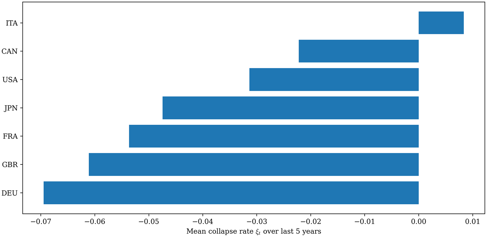
5.4. Recent collapse-rate behavior and the COVID-19 shock

To summarize the most recent portion of each series, the mean collapse rate is computed over the last five available observations,

$$ {\overline{\xi}}_{2019:2023}=\frac{1}{5}\sum \limits_{t=2019}^{2023}{\xi}_t. $$ xi bar 2019 colon 2023 equals 15 sigma summation t equals 20192023 xi t period

The averaging period is 2019–2023, comprising the final five annual observations. The interval includes the extraordinary 2020–2021 disruption of transport activity during the COVID-19 pandemic (Le Quéré et al., Reference Le Quéré, Jackson, Jones, Smith, Abernethy, Andrew, De-Gol, Willis, Shan, Canadell, Friedlingstein, Creutzig and Peters2020). It cannot be treated as a clean measure of endogenous contemporary fragility. Figure 4 displays the country-specific means for this interval.

Figure 4.

Mean collapse rate $ \overline{\xi} $ over the final five observations, 2019–2023. Positive values indicate an average decline in entropy over the interval and negative values an average increase. Because the interval includes the COVID-19 shock, the bars summarize recent path behavior but are not interpreted as country rankings of intrinsic structural fragility.

Horizontal bar chart of mean collapse rates for G7 countries over 2019–2023; Italy is slightly positive and the other six are negative, with Germany most negative. See long description.

Figure 4. Long description

The horizontal bars summarize mean collapse rates over the five observations from 2019 to 2023. Italy is slightly positive. Canada and the United States are modestly negative; France and Japan are more negative; the United Kingdom and Germany are the most negative. Because this interval contains the COVID-19 disruption and reopening, the chart is interpreted as recent path behaviour rather than as a ranking of intrinsic structural fragility.

The ranking remains descriptively informative: Germany and the United Kingdom show strongly negative averages, France and Japan moderately negative averages, Canada and the United States values close to zero on the negative side, and Italy a slightly positive value. Yet the pandemic created a large, externally imposed interruption in passenger and freight mobility, followed by uneven reopening and recovery. A five-observation average necessarily mixes the pre-shock endpoint, the collapse, and the rebound. Accordingly, Figure 4 is presented as a compact description of the recent sequence rather than as a measure of endogenous structural fragility.

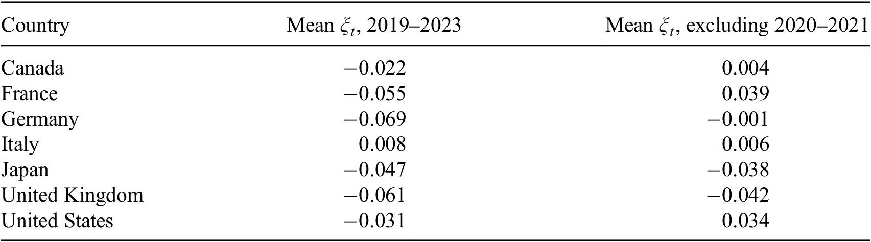
To assess directly how strongly this recent-period narrative depends on the pandemic years, Table 1 compares the baseline 2019–2023 mean with a simple non-COVID comparison computed from 2018, 2019, 2022, and 2023. The latter is not proposed as a definitive replacement—removing two adjacent years from such a short sequence also creates an irregular comparison—but it makes the sensitivity of the qualitative ranking explicit.

Table 1.

Sensitivity of recent mean collapse rates to the treatment of COVID-19 years

Table comparing mean collapse rates for 2019–2023 with means excluding the COVID-19 years 2020–2021 for seven G7 countries. See long description.

Table 1. Long description

Table 1 has seven country rows and two numerical columns. The 2019–2023 means are Canada −0.022, France −0.055, Germany −0.069, Italy 0.008, Japan −0.047, United Kingdom −0.061, and United States −0.031. Excluding 2020–2021, the corresponding means are Canada 0.004, France 0.039, Germany −0.001, Italy 0.006, Japan −0.038, United Kingdom −0.042, and United States 0.034. Canada, France, and the United States change sign, Germany moves close to zero, Japan and the United Kingdom remain negative, and Italy remains slightly positive.

The comparison materially changes the recent-period picture. Canada, France, and the United States change sign when 2020–2021 are excluded, while Germany moves close to zero; Japan and the United Kingdom remain negative, and Italy remains slightly positive. Thus, the short-window cross-country ranking is highly sensitive to the treatment of the pandemic. The appropriate substantive conclusion is heterogeneity in recent spectral paths under an exceptional global shock, not a stable ranking of endogenous resilience or fragility.

Overall, the results show recurrent, multi-decadal changes in the spectral organization of G7 transport-emission series. The descriptive evidence for a late-1990s alignment remains prominent, while Bayesian posterior width and modality reveal substantial country-specific uncertainty. The recent-period sensitivity results further demonstrate why unusual exogenous shocks must be separated from longer-run structural interpretation.

6. Discussion

The analysis shows that long-run transport-related CO₂ emissions contain changes in temporal organization that are not visible from level trends alone. Rolling spectral entropy identifies intervals in which detrended variability becomes more dispersed or more concentrated across the frequencies resolvable within a short annual window. Collapse rates identify rolling-window endpoints at which the estimated spectral concentration changes rapidly, and country-specific Bayesian models summarize the uncertainty surrounding a dominant mean-level division of each entropy sequence. The three components are complementary: entropy describes local organization, the collapse rate describes its direction of change, and the posterior distribution describes uncertainty in one parsimonious change-point summary.

The principal empirical finding is not a single universally dated G7 break. Rather, several countries exhibit low-entropy episodes and positive collapse-rate peaks in overlapping calendar regions, especially around the late 1990s, while the Bayesian evidence varies markedly in concentration and modality. This distinction resolves an important interpretive issue. Cross-country alignment in the descriptive indicators is meaningful evidence of temporal coherence, but it is not equivalent to formal evidence that all seven countries share one precisely dated transition. The present country-specific models do not estimate a common change point, and broad posteriors in Canada, Germany, Japan, and the United Kingdom require caution.

The substantive interpretation of spectral entropy must also remain bounded. In this application, a decline in $ {H}_t $ means that detrended variance within the current rolling window is concentrated in fewer resolvable Fourier components. It does not directly measure transport-system resilience, institutional fragility, or proximity to a tipping point. Similar mathematical indicators are useful in ecology, climate science, and remote sensing (Boettiger and Hastings, Reference Boettiger and Hastings2012; Zaccarelli et al., Reference Zaccarelli, Li, Petrosillo and Zurlini2013; De Keersmaecker et al., Reference De Keersmaecker, Lhermitte, Honnay, Farifteh, Somers and Coppin2014, Reference De Keersmaecker, Lhermitte, Tits, Honnay, Somers and Coppin2018; Lenton et al., Reference Lenton, Buxton, Armstrong McKay, Abrams, Boulton, Lees, Powell, Boers, Cunliffe and Dakos2022; Proverbio et al., Reference Proverbio, Skupin and Gonçalves2023), but anthropogenic emissions are generated by socio-technical and economic processes whose mechanisms differ from those of ecological state variables. The analogy is therefore methodological, not ontological.

Historical context nevertheless helps explain why overlapping calendar regions are plausible. Early-1980s entropy contractions coincide with the aftermath of the oil-price shocks, recession, changes in travel demand, and fuel-intensity adjustments documented across industrialized passenger-transport systems (Scholl et al., Reference Scholl, Schipper and Kiang1996; Greening, Reference Greening2004). The late-1990s alignment overlaps a period in which fuel prices and fuel-economy standards materially influenced new-vehicle efficiency, while European manufacturers operated under a voluntary commitment to reduce new-car CO₂ emissions (Fontaras and Samaras, Reference Fontaras and Samaras2007; Clerides and Zachariadis, Reference Clerides and Zachariadis2008). Late-2000s changes overlap the global financial crisis, the contraction of world trade and transport demand, and the associated temporary decline and subsequent rebound in global CO₂ emissions (International Transport Forum, 2009, 2010; Peters et al., Reference Peters, Marland, Le Quéré, Boden, Canadell and Raupach2012). These mechanisms are not identified by the model and should not be treated as causal findings. They provide historically grounded hypotheses that could be tested with policy indicators, fuel-price data, sectoral activity, or higher-frequency emissions.

The framework has several advantages. It is transparent, reproducible, and applicable when only a single long annual series is available. The normalization makes the entropy statistic comparable across countries with different emission scales. The full posterior distribution avoids concealing timing uncertainty behind one selected year. The combination of descriptive and probabilistic components also helps distinguish a visually striking trough from a statistically concentrated change-point posterior.

The same features create limitations. First, a 10-year annual window contains very little independent frequency information. With only a small number of Fourier ordinates, $ {H}_t $ is a coarse summary and can respond strongly to individual observations. The $ W=8 $ , $ 10 $ , and $ 12 $ comparisons in Appendix A examine sensitivity, but they cannot overcome the information limit imposed by annual data. The sensitivity analyses reduce the likelihood that the main calendar regions are artifacts of one selected preprocessing specification, but they do not fully separate persistent structural reorganization from all forms of transient disturbance or measurement error. Second, adjacent rolling windows overlap, so the resulting entropy sequence is serially dependent. The baseline independent Gaussian change-point likelihood may consequently understate posterior uncertainty. Third, the single-shift model cannot represent several breaks or a gradual transition. Broad and multimodal posteriors are consistent with this misspecification and should be reported rather than averaged into a definitive event. Fourth, the cross-country comparison is descriptive; no hierarchical model, common-change-point model, or causal panel design is estimated.

The recent-period analysis illustrates a related interpretive risk. The 2019–2023 average collapse rate includes the exceptional COVID-19 shock and subsequent reopening. It therefore summarizes the path through an extraordinary disruption rather than a stable national property. The sign changes reported in Table 1 when 2020–2021 are excluded demonstrate that short-window rankings are sensitive to the treatment of the pandemic. The interpretation is consequently limited to heterogeneity in recent spectral paths under a common global shock.

Future work can address these limitations in several ways. State-space or autoregressive change-point models could represent serial dependence directly. Multiple-change-point or product-partition formulations could distinguish several episodes rather than force one dominant split (Barry and Hartigan, Reference Barry and Hartigan1993; Chib, Reference Chib1998; Fearnhead, Reference Fearnhead2006; Fearnhead and Liu, Reference Fearnhead and Liu2007; Killick et al., Reference Killick, Fearnhead and Eckley2012; Truong et al., Reference Truong, Oudre and Vayatis2020). Hierarchical models could estimate shared and country-specific timing jointly, while higher-frequency emissions, mobility, fuel-price, freight, and policy data could improve both spectral resolution and substantive attribution. Out-of-sample simulation and controlled perturbation experiments would also help determine when spectral entropy responds to genuine regime change rather than preprocessing or transient noise.

The broader contribution is therefore methodological and comparative. Treating anthropogenic emissions as environmental signals makes it possible to ask how their temporal organization changes, not only whether their levels rise or fall. The present results support the use of spectral entropy and Bayesian uncertainty as diagnostic tools, provided that spectral concentration is not equated automatically with physical fragility and that broad posterior evidence is not converted into an artificially precise historical claim.

7. Conclusion

This study develops a reproducible framework for examining changes in the temporal organization of transport-related CO₂ emissions across the G7. Rolling spectral entropy summarizes whether detrended within-window variability is broadly distributed or concentrated across the frequencies resolvable in annual data. The collapse rate identifies rapid changes in that concentration, and country-specific Bayesian mean-shift models quantify uncertainty in a parsimonious transition-year summary.

The empirical results reveal recurrent low-entropy episodes and several periods of cross-country alignment, including a visually prominent late-1990s interval. That alignment is an important descriptive finding, but it is not equivalent to a precisely identified common G7 change point. Posterior evidence differs substantially across countries: some distributions are comparatively concentrated, while others are broad or multimodal. The interpretation therefore distinguishes descriptive coherence from formal timing certainty.

The analysis also clarifies what the indicators do not establish. Spectral entropy is not a direct measure of resilience or fragility, the single-shift model does not imply that only one historical transition occurred, and the recent 2019–2023 collapse-rate average cannot be separated from the COVID-19 shock. These limitations are especially important because the annual rolling windows provide coarse frequency resolution and induce serial dependence in the entropy sequence.

Despite these constraints, the framework offers a useful diagnostic complement to level-based emissions analysis. It can identify intervals that merit closer historical or sectoral investigation and can be extended to other environmental and socio-technical time series. Future research should use higher-frequency data, multiple-change-point or autoregressive formulations, hierarchical cross-country models, and richer covariates to test the mechanisms underlying the descriptive patterns documented here.

Open peer review

To view the open peer review materials for this article, please visit http://doi.org/10.1017/eds.2026.10064.

AI use declaration

The author used AI (ChatGPT) only to assist with language editing. No AI tool was used to generate or analyze data, run estimations, or produce quantitative results. The author takes full responsibility for the final manuscript.

Author contribution

Conceptualization: T.N. Data curation: T.N. Formal analysis: T.N. Methodology: T.N. Software: T.N. Visualization: T.N. Writing—original draft: T.N. Writing—review and editing: T.N.

Code availability

All analysis scripts, including the spectral-entropy computation and Bayesian change-point inference, are openly accessible at: https://github.com/g7-spectral-entropy/spectral-entropy-g7.

The repository contains: (i) Python source files for the baseline spectral-entropy analysis, sensitivity analyses, and Bayesian change-point inference; (ii) compact numerical summary tables; and (iii) an environment file ensuring computational reproducibility. Further computational and model-reporting details are provided in Appendix D.

Competing interests

The author declares no competing interests.

Data availability statement

The environmental time-series data used in this study are derived from the World Bank World Development Indicators repository (indicator EN.GHG.CO2.TR.MT.CE.AR5), which is publicly available at: https://data.worldbank.org/indicator/EN.GHG.CO2.TR.MT.CE.AR5.

The processed panel dataset generated during the analysis (e.g., spectral-entropy and collapse-rate series) is openly available in the associated GitHub repository: https://github.com/g7-spectral-entropy/spectral-entropy-g7.

Ethics statement

This study uses publicly available, aggregated environmental data and involves no human or animal subjects.

Funding statement

This research received no specific grant from any funding agency, commercial, or not-for-profit sectors.

Appendix A. Robustness of spectral-entropy indicators

A central concern in applying entropy-based indicators to annual environmental time series is sensitivity to rolling-window length and detrending. The analysis therefore compares $ W=8 $ , $ 10 $ , and $ 12 $ years and alternative detrending choices (linear, local polynomial, and differencing). These checks evaluate whether the broad timing of entropy contractions persists under reasonable preprocessing changes; they do not eliminate the limited frequency resolution inherent in short annual windows.

The main trough regions remain visible under several specifications, but their exact year, depth, and cross-country alignment vary. The sensitivity analysis therefore supports the existence of recurring changes in local spectral concentration while cautioning against interpreting a 1-year difference as substantively precise evidence. In particular, similarity around the late 1990s is best described as a robust calendar region rather than a universally fixed transition date.

Figure A1 shows, for each country, the observed transport-related CO₂ series, the baseline entropy sequence, and the associated collapse rate. The panels make clear that entropy movements should be interpreted alongside the original data. A trough can be influenced by a sustained adjustment, an exceptional observation, endpoint behavior, or the interaction of several consecutive years.

Figure A1.

Country-level transport-related CO₂ series (top), spectral entropy $ {H}_t $ (middle), and collapse rate $ {\xi}_t $ (bottom) under the baseline specification. Recurring troughs and peaks are visible in several countries, but their exact timing and magnitude differ. The figure is used to assess whether the entropy patterns correspond to persistent features of the underlying paths rather than to one isolated plotted statistic.

Seven-country panel figure showing transport CO2 emissions, spectral entropy, and collapse rate under the baseline specification for Canada, France, Germany, Italy, Japan, the UK, and the US. See long description.

Figure A1. Long description

The figure contains seven country panels. Each panel has three aligned time-series plots: observed transport-related CO2 emissions at the top, baseline normalized spectral entropy in the middle, and collapse rate at the bottom. The panels show that entropy troughs and collapse-rate peaks occur repeatedly but differ in exact timing and magnitude across countries. Reading the three series together helps distinguish persistent features of the underlying emissions path from isolated movements in a single diagnostic.

Figure A2 provides the direct baseline comparison for $ W=8 $ , $ 10 $ , and $ 12 $ . The curves do not coincide exactly, as expected from changes in frequency resolution and window composition, but broad periods of spectral concentration recur under more than one window length in several countries. The evidence therefore supports interpretation at the level of calendar regions rather than exact one-year dates.

Figure A2.

Sensitivity of normalized spectral entropy to rolling-window length. Each panel compares $ W=8 $ , $ 10 $ , and $ 12 $ using the same emissions series and the baseline 5-year moving-average residual construction. Recurrence of broad trough regions supports calendar-region comparisons, while variation in exact minima illustrates the limited temporal and frequency resolution of short annual windows.

Seven-country sensitivity panels comparing normalized spectral entropy under rolling windows of 8, 10, and 12 years; broad trough regions recur but exact minima vary. See long description.

Figure A2. Long description

Seven panels, one for each G7 country, compare normalized spectral-entropy paths calculated with rolling-window lengths of 8, 10, and 12 years using the same baseline detrending method. The three curves do not coincide exactly. However, broad periods of spectral concentration recur under more than one window length in several countries. Differences in exact minima illustrate the limited temporal and frequency resolution of short annual windows.

Figure A3 compares the baseline 5-year moving-average residual construction with local linear detrending, local polynomial detrending, and first differencing at $ W=10 $ . Detrending affects the level, depth, and exact timing of some minima, but recurring periods of spectral concentration remain visible under more than one specification. The comparison therefore argues against attributing the principal patterns solely to one preprocessing rule, while demonstrating that preprocessing uncertainty remains material.

Figure A3.

Sensitivity of normalized spectral entropy to detrending at $ W=10 $ . The panels compare the baseline moving-average residual construction, local linear detrending, local polynomial detrending, and first differencing. Recurrence of broad trough regions across several specifications provides evidence that the main descriptive patterns are not generated exclusively by one detrending choice; differences in exact timing and depth remain part of the uncertainty.

Seven-country sensitivity panels comparing four detrending methods at a 10-year window: moving-average residuals, local linear, local polynomial, and first differencing. See long description.

Figure A3. Long description

Seven panels, one for each G7 country, compare normalized spectral entropy at a 10-year rolling window under four preprocessing choices: the baseline five-year moving-average residual construction, local linear detrending, local polynomial detrending, and first differencing. Detrending changes the level, depth, and exact timing of some entropy minima, but broad trough regions recur under multiple specifications. The figure therefore shows both robustness of broad calendar regions and material preprocessing uncertainty.

The sensitivity evidence does not prove that every trough represents a structural break, nor does it identify a causal driver. It shows directly that the principal calendar regions are not wholly dependent on one selected window length or one detrending rule. These robustness checks address sensitivity to window length and detrending, but they do not constitute a formal statistical test that distinguishes persistent structural change from every possible transient shock or measurement disturbance. Accordingly, the entropy contractions are interpreted as reproducible descriptive features of the observed series rather than as independently validated causal regime changes. That is the appropriate robustness claim for a short annual spectral analysis.

Appendix B. Low- and high-frequency variability decomposition

Spectral entropy summarizes the entire normalized power distribution, so a low value can arise from concentration in different portions of the spectrum. To aid interpretation, the normalized power is divided into lower-frequency and higher-frequency components. This decomposition is descriptive because a 10-year annual window cannot resolve long periodicities precisely.

Periods of lower entropy are generally associated with a larger share of power in the lower-frequency portion of the available spectrum. This pattern is consistent with more persistent within-window variation, but it should not be interpreted as the detection of a well-estimated decadal cycle. The frequency grid is coarse, and the band division is sensitive to the window length. Higher-frequency power remains relevant in several countries and cannot be dismissed as measurement noise.

The decomposition therefore supports a limited conclusion: the entropy troughs are often connected to changes in the balance between slower and faster components of the detrended sequence. It does not establish that shared policy, technology, or macroeconomic forces are the unique cause of those changes. Such attribution requires external covariates and a model designed for causal inference.

Appendix C. Bayesian change-point diagnostics and posterior inference

The Bayesian analysis provides country-specific posterior distributions for the location of one mean shift in each entropy sequence. Its purpose is to quantify uncertainty in a parsimonious summary, not to assert that the true history contains only one abrupt transition. The appendix therefore emphasizes posterior spread and modality as well as the plotted posterior mean.

C.1 Model specification and fitted trajectories

The model is

with the priors and sampling settings reported in Section 4.4. The fitted trajectories in Figure C1 display the entropy sequence, posterior summaries of the two regime means, and the posterior-mean change year. These graphical summaries are convenient, but a vertical line should not be read as evidence that the plotted year is the posterior mode or that uncertainty is narrow.

Figure C1.

Country-specific Bayesian single-mean-shift fits. Blue lines show annual entropy $ {H}_t $ , vertical dashed lines show posterior-mean transition years, and horizontal segments summarize pre- and post-shift mean levels. The full posterior distributions in Figure C2 are required for assessing timing uncertainty.

Seven-panel Bayesian single-mean-shift fits for the G7, with annual entropy, posterior-mean transition lines, and pre- and post-shift mean levels. See long description.

Figure C1. Long description

Seven panels show the fitted country-specific single-mean-shift model for Canada, France, Germany, Italy, Japan, the United Kingdom, and the United States. Each panel plots annual spectral entropy, a vertical dashed line at the posterior-mean transition year, and horizontal segments for the estimated pre- and post-shift mean levels. The panels are graphical summaries only: a vertical line does not imply that the plotted year is the posterior mode or that uncertainty is narrow. Timing uncertainty is assessed in Figure 2 and Table 1.

C.2 Posterior distributions of transition years

Figure C2 displays the complete posterior distributions $ p\left(\tau |{H}_{1:T}\right) $ . The principal result is heterogeneity in identification. France, Italy, and the United States show comparatively more concentrated probability in particular calendar regions. Canada, Germany, Japan, and the United Kingdom show broader or multimodal distributions, indicating several plausible divisions or a gradual sequence that is poorly represented by one abrupt mean shift.

Figure C2.

Posterior distributions of country-specific change-point years. Vertical dashed lines mark posterior means; the corresponding 90% credible intervals are reported in Table C1. All panels use the same calendar-year limits so that spread and modality are directly comparable. Broad or multimodal panels indicate weak identification of a unique transition year.

Seven-panel posterior distributions for country-specific change-point years, showing concentrated, broad, and multi-modal patterns across the G7. See long description.

Figure C2. Long description

Seven panels show posterior probability distributions for the change-point year on common calendar-year axes. Italy is comparatively concentrated around the late 2000s. France has an early-1980s mode with a long upper tail, and the United States has a late-2000s mode with substantial lower-tail uncertainty. Canada, Germany, Japan, and the United Kingdom have broad or multi-modal distributions. Vertical dashed lines mark posterior means, while Table 1 reports modal years and 90% credible intervals. The broad and multi-modal panels indicate weak identification of a unique transition year.

This heterogeneity changes the substantive interpretation. Recurring probability mass near the early 1980s, late 1990s, and late 2000s can be compared across countries, but it does not constitute evidence for one synchronized G7 transition. In a broad or multimodal posterior, the posterior mean may lie between modes or at a year with relatively low probability. For that reason, the posterior mean is retained only as a summary compatible with the fitted figures; posterior width, the modal year, and the 90% credible interval govern the interpretation.

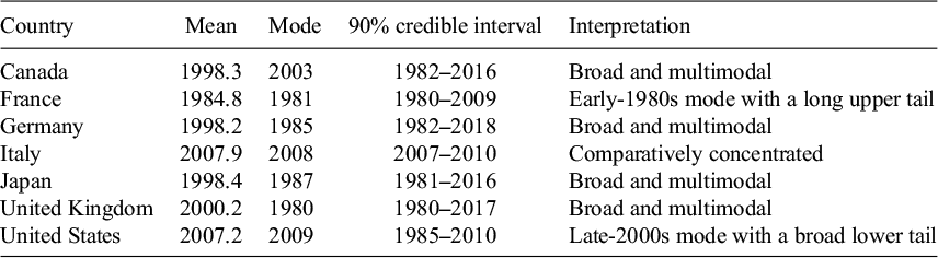
Table C1 makes clear why the posterior mean is not treated as a declared change year. Italy has a comparatively concentrated posterior, whereas Canada, Germany, Japan, and the United Kingdom have broad or multimodal distributions. France retains an early-1980s mode with a long upper tail, and the United States has a late-2000s mode with substantial lower-tail uncertainty. The modal year and interval are therefore reported alongside the mean rather than replacing the complete posterior distribution.

Table C1.

Country-specific posterior summaries for the single-mean-shift model

Table of posterior mean, mode, 90% credible interval, and interpretation of the country-specific change-point year for each G7 country. See long description.

Table C1. Long description

Table 1 reports posterior summaries for the single-mean-shift model. Canada: mean 1998.3, mode 2003, 90% interval 1982–2016, broad and multi-modal. France: 1984.8, mode 1981, 1980–2009, early-1980s mode with a long upper tail. Germany: 1998.2, mode 1985, 1982–2018, broad and multi-modal. Italy: 2007.9, mode 2008, 2007–2010, comparatively concentrated. Japan: 1998.4, mode 1987, 1981–2016, broad and multi-modal. United Kingdom: 2000.2, mode 1980, 1980–2017, broad and multi-modal. United States: 2007.2, mode 2009, 1985–2010, late-2000s mode with a broad lower tail.

C.3 Multiple and hierarchical extensions

No multiple-change-point, common-change-point, or partially pooled model is estimated in this study. These extensions are nevertheless natural next steps. A multiple-change-point formulation could represent separate early-1980s, late-1990s, and late-2000s episodes without forcing them into one dominant split (Barry and Hartigan, Reference Barry and Hartigan1993; Chib, Reference Chib1998; Fearnhead, Reference Fearnhead2006; Fearnhead and Liu, Reference Fearnhead and Liu2007; Killick et al., Reference Killick, Fearnhead and Eckley2012; Truong et al., Reference Truong, Oudre and Vayatis2020). A hierarchical model could estimate the extent of shared timing while allowing country-specific deviations.

Such models would answer questions that the present analysis cannot resolve: whether a common G7 component exists, which countries lead or lag that component, and whether broad country-level posteriors result from gradual adjustment or several discrete shifts. They are therefore presented as future methodological extensions rather than as analyses already performed.

Appendix D. Computational reproducibility and model-reporting details

The computational archive contains the G7 source extract, the derived panel of $ {H}_t $ and $ {\xi}_t $ , the country-level change-point summaries, Python source files, compact numerical summary tables, and the software environment specification. The entropy implementation uses the documented 5-year moving-average residual construction, a rolling window of up to 10 observations with a 6-observation minimum at the beginning of the series, a Hann taper, zero-padding to the next power of 2, a real Fourier transform, within-window power normalization, and normalized Shannon entropy. The Bayesian implementation fits each country independently with PyMC using two chains, 2000 tuning iterations, and 2000 retained draws per chain, with target_accept = 0.9 and random seed 123.

The repository is intended to permit full regeneration of the derived series, figures, and change-point summaries. The posterior histograms and interval summaries are produced from the saved workflow. Reproducibility is therefore based on the public code, input data, environment specification, and fixed random seed rather than on undocumented manual adjustments.

Footnotes

This research article was awarded Open Data and Open Materials badges for transparent practices. See the Data Availability Statement for details.

References

Barry, D and Hartigan, JA (1993) A bayesian analysis for change point problems. Journal of the American Statistical Association 88(421), 309–319. https://doi.org/10.1080/01621459.1993.10594323.CrossRef Google Scholar

Boettiger, C and Hastings, A (2012) Quantifying limits to detection of early warning for critical transitions. Journal of the Royal Society Interface 9(75), 2527–2539. https://doi.org/10.1098/rsif.2012.0125.CrossRef Google Scholar PubMed

Chib, S (1998) Estimation and comparison of multiple change-point models. Journal of Econometrics 86(2), 221–241. https://doi.org/10.1016/S0304-4076(97)00115-2.CrossRef Google Scholar

Clerides, S and Zachariadis, T (2008) The effect of standards and fuel prices on automobile fuel economy: An international analysis. Energy Economics 30(5), 2657–2672. https://doi.org/10.1016/j.eneco.2008.06.001.CrossRef Google Scholar

Creutzig, F, Jochem, P, Edelenbosch, OY, Mattauch, L, van Vuuren, DP, McCollum, D and Minx, J (2015) Transport: A roadblock to climate change mitigation? Science 350(6263), 911–912. https://doi.org/10.1126/science.aac8033.CrossRef Google Scholar PubMed

Dakos, V, Carpenter, SR, Brock, WA, Ellison, AM, Guttal, V, Ives, AR, Kéfi, S, Livina, V, Seekell, DA, van Nes, EH and Scheffer, M (2012) Methods for detecting early warnings of critical transitions in time series illustrated using simulated ecological data. PLoS One 7(7), e41010. https://doi.org/10.1371/journal.pone.0041010.CrossRef Google Scholar PubMed

De Keersmaecker, W, Lhermitte, S, Honnay, O, Farifteh, J, Somers, B and Coppin, P (2014) How to measure ecosystem stability? An evaluation of the reliability of stability metrics based on remote sensing time series across the major global ecosystems. Global Change Biology 20(7), 2149–2161. https://doi.org/10.1111/gcb.12495.CrossRef Google Scholar PubMed

De Keersmaecker, W, Lhermitte, S, Tits, L, Honnay, O, Somers, B and Coppin, P (2018) Resilience and the reliability of spectral entropy to assess ecosystem stability. Global Change Biology 24(1), e393–e394. https://doi.org/10.1111/gcb.12799.CrossRef Google Scholar PubMed

Falduto, C, Wartmann, S and Rocha, M (2020). Reporting national ghg inventories through common reporting tables (crts): An assessment of crt reporting options through worked examples. Paris: OECD Publishing. Technical Report 2020/03.Google Scholar

Fearnhead, P (2006) Exact and efficient bayesian inference for multiple changepoint problems. Statistics and Computing 16(2), 203–213. https://doi.org/10.1007/s11222-006-8450-8.CrossRef Google Scholar

Fearnhead, P and Liu, Z (2007) On-line inference for multiple changepoint problems. Journal of the Royal Statistical Society Series B: Statistical Methodology 69(4), 589–605. https://doi.org/10.1111/j.1467-9868.2007.00601.x.CrossRef Google Scholar

Fontaras, G and Samaras, Z (2007) A quantitative analysis of the european automakers’ voluntary commitment to reduce co2 emissions from new passenger cars based on independent experimental data. Energy Policy 35(4), 2239–2248. https://doi.org/10.1016/j.enpol.2006.07.012.CrossRef Google Scholar

Friedlingstein, P, O’Sullivan, M, Jones, MW, Andrew, RM, Bakker, DCE, Hauck, J, Landschützer, P, le Quéré, C, Luijkx, IT, Peters, GP, Peters, W, Pongratz, J, Schwingshackl, C, Sitch, S, Canadell, JG, Ciais, P, Jackson, RB, Alin, SR, Anthoni, P, Barbero, L, Bates, NR, Becker, M, Bellouin, N, Decharme, B, Bopp, L, Brasika, IBM, Cadule, P, Chamberlain, MA, Chandra, N, Chau, TTT, Chevallier, F, Chini, LP, Cronin, M, Dou, X, Enyo, K, Evans, W, Falk, S, Feely, RA, Feng, L, Ford, DJ, Gasser, T, Ghattas, J, Gkritzalis, T, Grassi, G, Gregor, L, Gruber, N, Gürses, Ö, Harris, I, Hefner, M, Heinke, J, Houghton, RA, Hurtt, GC, Iida, Y, Ilyina, T, Jacobson, AR, Jain, A, Jarníková, T, Jersild, A, Jiang, F, Jin, Z, Joos, F, Kato, E, Keeling, RF, Kennedy, D, Klein Goldewijk, K, Knauer, J, Korsbakken, JI, Körtzinger, A, Lan, X, Lefèvre, N, Li, H, Liu, J, Liu, Z, Ma, L, Marland, G, Mayot, N, McGuire, PC, McKinley, GA, Meyer, G, Morgan, EJ, Munro, DR, Nakaoka, SI, Niwa, Y, O’Brien, KM, Olsen, A, Omar, AM, Ono, T, Paulsen, M, Pierrot, D, Pocock, K, Poulter, B, Powis, CM, Rehder, G, Resplandy, L, Robertson, E, Rödenbeck, C, Rosan, TM, Schwinger, J, Séférian, R, Smallman, TL, Smith, SM, Sospedra-Alfonso, R, Sun, Q, Sutton, AJ, Sweeney, C, Takao, S, Tans, PP, Tian, H, Tilbrook, B, Tsujino, H, Tubiello, F, van der Werf, GR, van Ooijen, E, Wanninkhof, R, Watanabe, M, Wimart-Rousseau, C, Yang, D, Yang, X, Yuan, W, Yue, X, Zaehle, S, Zeng, J and Zheng, B (2023) Global carbon budget 2023. Earth System Science Data 15(12), 5301–5369. https://doi.org/10.5194/essd-15-5301-2023.CrossRef Google Scholar

Government of Japan (2019) National greenhouse gas inventory report of japan 2019. Tsukuba, Japan. Greenhouse Gas Inventory Office of Japan, National Institute for Environmental Studies. Submitted to the United Nations Framework Convention on Climate Change.Technical report.Google Scholar

Greening, LA (2004) Effects of human behavior on aggregate carbon intensity of personal transportation: Comparison of 10 oecd countries for the period 1970–1993. Energy Economics 26(1), 1–30. https://doi.org/10.1016/j.eneco.2003.05.001.CrossRef Google Scholar

Inouye, T, Shinosaki, K, Sakamoto, H, Toi, S, Ukai, S, Iyama, A, Katsuda, Y and Hirano, M (1991) Quantification of eeg irregularity by use of the entropy of the power spectrum. Electroencephalography and Clinical Neurophysiology 79(3), 204–210. https://doi.org/10.1016/0013-4694(91)90138-T.CrossRef Google Scholar PubMed

International Transport Forum (2009) Transport outlook 2009: Globalisation, crisis and transport. In Discussion Paper. Paris: OECD/International Transport Forum.Google Scholar

International Transport Forum (2010). Trends in the transport sector 2010. Paris: OECD. Technical report. https://doi.org/10.1787/trend_transp-2010-en.CrossRef Google Scholar

International Transport Forum (2023) ITF Transport Outlook 2023. Paris: OECD Publishing. https://doi.org/10.1787/b6cc9ad5-en.Google Scholar

IPCC (2021) Climate Change 2021: The Physical Science Basis. Cambridge, UK and New York, NY: Cambridge University Press.Google Scholar

Killick, R, Fearnhead, P and Eckley, IA (2012) Optimal detection of changepoints with a linear computational cost. Journal of the American Statistical Association 107(500), 1590–1598. https://doi.org/10.1080/01621459.2012.737745.CrossRef Google Scholar

Le Quéré, C, Jackson, RB, Jones, MW, Smith, AJP, Abernethy, S, Andrew, RM, De-Gol, AJ, Willis, DR, Shan, Y, Canadell, JG, Friedlingstein, P, Creutzig, F and Peters, GP (2020) Temporary reduction in daily global co2 emissions during the covid-19 forced confinement. Nature Climate Change 10(7), 647–653. https://doi.org/10.1038/s41558-020-0797-x.CrossRef Google Scholar

Lenton, TM, Buxton, JE, Armstrong McKay, DI, Abrams, JF, Boulton, CA, Lees, KJ, Powell, TWR, Boers, N, Cunliffe, AM and Dakos, V (2022) A resilience sensing system for the biosphere. Philosophical Transactions of the Royal Society B: Biological Sciences 377(1857), 20210383. https://doi.org/10.1098/rstb.2021.0383.CrossRef Google Scholar PubMed

Li, X, Ren, A and Li, Q (2022) Exploring patterns of transportation-related co2 emissions using machine learning methods. Sustainability 14(8), 4588. https://doi.org/10.3390/su14084588.CrossRef Google Scholar

Lund, RB, Beaulieu, C, Killick, R, Lu, Q and Shi, X (2023) Good practices and common pitfalls in climate time series changepoint techniques: A review. Journal of Climate 36(23), 8041–8057. https://doi.org/10.1175/JCLI-D-22-0954.1.CrossRef Google Scholar

Peters, GP, Andrew, RM, Canadell, JG, Fuss, S, Jackson, RB, Korsbakken, JI, Le Quéré, C and Nakicenovic, N (2017) Key indicators to track current progress and future ambition of the Paris agreement. Nature Climate Change 7(2), 118–122. https://doi.org/10.1038/nclimate3202.CrossRef Google Scholar

Peters, GP, Marland, G, Le Quéré, C, Boden, T, Canadell, JG and Raupach, MR (2012) Rapid growth in co2 emissions after the 2008–2009 global financial crisis. Nature Climate Change 2(1), 2–4. https://doi.org/10.1038/nclimate1332.CrossRef Google Scholar

Proverbio, D, Skupin, A and Gonçalves, J (2023) Systematic analysis and optimization of early warning signals for critical transitions using distribution data. iScience 26(7), 107156. https://doi.org/10.1016/j.isci.2023.107156.CrossRef Google Scholar PubMed

Reeves, J, Chen, J, Wang, XL, Lund, R and Lu, QQ (2007) A review and comparison of changepoint detection techniques for climate data. Journal of Applied Meteorology and Climatology 46(6), 900–915. https://doi.org/10.1175/JAM2493.1.CrossRef Google Scholar

Scheffer, M, Bascompte, J, Brock, WA, Brovkin, V, Carpenter, SR, Dakos, V, Held, H, van Nes, EH, Rietkerk, M and Sugihara, G (2009) Early-warning signals for critical transitions. Nature 461(7260), 53–59. https://doi.org/10.1038/nature08227.CrossRef Google Scholar PubMed

Scholl, L, Schipper, L and Kiang, N (1996) Co2 emissions from passenger transport: A comparison of international trends from 1973 to 1992. Energy Policy 24(1), 17–30. https://doi.org/10.1016/0301-4215(95)00148-4.CrossRef Google Scholar

Shannon, CE (1948) A mathematical theory of communication. Bell System Technical Journal 27(3), 379–423. 10.1002/j.1538-7305.1948.tb01338.x.10.1002/j.1538-7305.1948.tb01338.xCrossRef Google Scholar

Sims, R, Schaeffer, R, Creutzig, F, Cruz-Núñez, X, D’Agosto, M, Dimitriu, D, Figueroa Meza, MJ, Fulton, L, Kobayashi, S, Lah, O, McKinnon, A, Newman, P, Ouyang, M, Schauer, JJ, Sperling, D and Tiwari, G (2014) Transport. In Edenhofer, O, Pichs-Madruga, R, Sokona, Y, Farahani, E, Kadner, S, Seyboth, K, Adler, A, Baum, I, Brunner, S, Eickemeier, P, Kriemann, B, Savolainen, J, Schlömer, S, von Stechow, C, Zwickel, T and Minx, JC (eds), Climate Change 2014: Mitigation of Climate Change. Cambridge University Press, Cambridge, United Kingdom and New York, NY, USA, pp. 599–670.Google Scholar

Truong, C, Oudre, L and Vayatis, N (2020) Selective review of offline change point detection methods. Signal Processing 167, 107299. https://doi.org/10.1016/j.sigpro.2019.107299.CrossRef Google Scholar

World Bank (2024) World development indicators: Carbon dioxide (co2) emissions from transport (energy) (mt co2e). https://data.worldbank.org/indicator/EN.GHG.CO2.TR.MT.CE.AR5. Indicator EN.GHG.CO2.TR.MT.CE.AR5; accessed 12 july 2026Google Scholar

Zaccarelli, N, Li, B-L, Petrosillo, I and Zurlini, G (2013) Order and disorder in ecological time-series: Introducing normalized spectral entropy. Ecological Indicators 28, 22–30. https://doi.org/10.1016/j.ecolind.2011.07.008.CrossRef Google Scholar

Zanin, M and Olivares, F (2021) Ordinal patterns-based methodologies for distinguishing chaos from noise in discrete time series. Communications Physics 4(1), 190. https://doi.org/10.1038/s42005-021-00696-z.CrossRef Google Scholar

Figure 1. Long-run evolution of normalized spectral entropy Ht$ {H}_t $ for transport-related CO2 emissions across the G7, 1970–2023. Each plotted point corresponds to the endpoint of a rolling window. Lower values indicate greater concentration of detrended within-window variance in a smaller subset of resolvable Fourier components. Several countries exhibit low-entropy episodes in similar calendar regions, but the timing, depth, and posterior support differ across countries.Figure 1. long description.

Figure 2. Collapse-rate series ξt=−ΔHt$ {\xi}_t=-\Delta {H}_t $ for the G7. Each point records the year-to-year change in rolling spectral entropy. Positive peaks mark rapid local declines in entropy. Several countries show peaks in or near 1998–2000, providing descriptive evidence of cross-country temporal alignment; the figure does not by itself establish a common transition year or a shared causal mechanism.Figure 2. long description.

Figure 3. Country-specific Bayesian single-mean-shift fits for representative G7 entropy sequences. The vertical dashed line is the posterior-mean change year and the horizontal segments are posterior summaries of the two regime means. These lines summarize the fitted model but should be interpreted together with the full posterior distributions in Appendix C. Broad or multimodal posteriors imply that no single calendar year is strongly identified, even when the posterior mean is plotted.Figure 3. long description.

Figure 4. Mean collapse rate ξ¯$ \overline{\xi} $ over the final five observations, 2019–2023. Positive values indicate an average decline in entropy over the interval and negative values an average increase. Because the interval includes the COVID-19 shock, the bars summarize recent path behavior but are not interpreted as country rankings of intrinsic structural fragility.Figure 4. long description.

Table 1. Sensitivity of recent mean collapse rates to the treatment of COVID-19 yearsTable 1. long description.

Figure A1. Country-level transport-related CO2 series (top), spectral entropy Ht$ {H}_t $ (middle), and collapse rate ξt$ {\xi}_t $ (bottom) under the baseline specification. Recurring troughs and peaks are visible in several countries, but their exact timing and magnitude differ. The figure is used to assess whether the entropy patterns correspond to persistent features of the underlying paths rather than to one isolated plotted statistic.Figure A1. long description.

Figure A2. Sensitivity of normalized spectral entropy to rolling-window length. Each panel compares W=8$ W=8 $, 10$ 10 $, and 12$ 12 $ using the same emissions series and the baseline 5-year moving-average residual construction. Recurrence of broad trough regions supports calendar-region comparisons, while variation in exact minima illustrates the limited temporal and frequency resolution of short annual windows.Figure A2. long description.

Figure A3. Sensitivity of normalized spectral entropy to detrending at W=10$ W=10 $. The panels compare the baseline moving-average residual construction, local linear detrending, local polynomial detrending, and first differencing. Recurrence of broad trough regions across several specifications provides evidence that the main descriptive patterns are not generated exclusively by one detrending choice; differences in exact timing and depth remain part of the uncertainty.Figure A3. long description.

Figure C1. Country-specific Bayesian single-mean-shift fits. Blue lines show annual entropy Ht$ {H}_t $, vertical dashed lines show posterior-mean transition years, and horizontal segments summarize pre- and post-shift mean levels. The full posterior distributions in Figure C2 are required for assessing timing uncertainty.Figure C1. long description.

Figure C2. Posterior distributions of country-specific change-point years. Vertical dashed lines mark posterior means; the corresponding 90% credible intervals are reported in Table C1. All panels use the same calendar-year limits so that spread and modality are directly comparable. Broad or multimodal panels indicate weak identification of a unique transition year.Figure C2. long description.

Table C1. Country-specific posterior summaries for the single-mean-shift modelTable C1. long description.

Author comment: Detecting structural transitions in climate-sensitive environmental signals using spectral entropy and Bayesian change-point inference — R0/PR1

Published online by Cambridge University Press: 10 October 2026

DOI: https://doi.org/10.1017/eds.2026.10064.pr1

Tomoo Noguchi

School of Social Sciences, Waseda University, Japan

Revision round: 0

Role: author

Comments

Professor Tomoo Noguchi

School of Social Sciences, Waseda University

1-6-1 Nishiwaseda, Shinjuku-ku

Tokyo 169-8050

Japan

Email: tomo@waseda.jp

ORCID: 0009-0008-2222-7165

December 3, 2025

________________________________________

Editors-in-Chief

Environmental Data Science

Cambridge University Press

Dear Editors,

I am pleased to submit my manuscript entitled “Detecting Structural Transitions in Climate-Sensitive Environmental Signals Using Spectral Entropy and Bayesian Change-Point Inference” for consideration in Environmental Data Science. The manuscript develops a fully reproducible, structure-aware analytical framework for detecting long-run reorganizations in anthropogenic environmental signals using frequency-domain information metrics and Bayesian uncertainty quantification.

This study aligns closely with the journal’s mission to advance transparent, data-driven approaches for understanding complex environmental systems. Its central contributions include:

- Introducing a unified analytical pipeline that integrates spectral entropy, collapse-rate dynamics, autoregressive persistence, and Bayesian estimation of transition years to quantify structural variability in environmental time series.

- Demonstrating that anthropogenic CO₂ emissions, treated as environmental signals, possess internal temporal organization that can undergo structural reorganizations analogous to those observed in biophysical systems.

- Identifying recurrent entropy troughs and coordinated structural transitions across the G7 economies from 1970–2023, including a pronounced synchronized contraction during 1998–2000 strongly supported by posterior distributions.

- Providing a generalizable and system-agnostic framework applicable to climatic, ecological, hydrological, and socio-technical signals commonly analyzed in Environmental Data Science.

- Ensuring full computational reproducibility through openly accessible data, code, and analysis notebooks hosted on GitHub.

To the best of my knowledge, this is the first study to offer a spectral-entropy-based characterization of structural transitions in anthropogenic environmental signals across advanced economies. The findings underscore the value of structure-aware environmental monitoring and highlight coordinated, system-level reorganizations that cannot be detected through level-based indicators alone.

I confirm that the manuscript is original, has not been submitted elsewhere, and contains no conflicts of interest. All analyses were conducted by the author, and all necessary approvals have been obtained.

Given the methodological contributions, cross-system relevance, and strong alignment with the scope of Environmental Data Science, I respectfully request that the manuscript be considered for publication.

Thank you very much for your time and consideration. I look forward to your response.

Sincerely,

Professor Tomoo Noguchi

School of Social Sciences, Waseda University

Email: tomo@waseda.jp

ORCID: 0009-0008-2222-7165

Review: Detecting structural transitions in climate-sensitive environmental signals using spectral entropy and Bayesian change-point inference — R0/PR2

Published online by Cambridge University Press: 10 October 2026

DOI: https://doi.org/10.1017/eds.2026.10064.pr2

Reviewer_1

Date of review: 18 March 2026

Revision round: 0

Role: reviewer

Recommendation/decision: major-revision

Conflict of interest statement

Reviewer declares none.

Comments

This paper introduces an analytical framework for detecting structural transitions in transport-related CO2 emissions across G7 countries, combining spectral entropy as a measure of structural variability with Bayesian change-point inference to identify transition years. The work addresses an important problem in environmental data science. However, the proposed framework requires stronger methodological justification in several areas, and the manuscript would benefit from editorial revision to reduce redundancy and improve clarity.

Major Comments

1. The paper applies spectral entropy to quantify structural change in transport-related CO2 emissions, but the interpretive basis of this indicator in the present application is insufficiently established. The framework detrends and normalizes the raw series within each rolling window, removing all level information before computing the Fourier transform. Spectral entropy then measures how much the resulting normalized residuals concentrate in a small number of frequencies. While this approach is well-motivated in ecological and remote-sensing contexts, it is unclear what the extracted Ht signal captures in the specific context of anthropogenic CO2 emissions: does it reflect meaningful structural patterns in human-driven forcing, or primarily noise and preprocessing artifacts? The reliance on ecological analogies is noted but does not substitute for domain-specific justification. The author should clarify what a decline in Ht concretely implies for CO2 emission dynamics, and provide evidence that the indicator is sensitive to genuine structural change rather than to short-term fluctuations or measurement noise.

2. The Bayesian change-point model assumes a single mean shift between two constant levels with i.i.d. normal noise, which is a highly restrictive specification given the data. Figure 3 makes clear that the Ht series exhibits clear autocorrelation, oscillatory behaviour, and likely multiple structural shifts rather than a single transition — all of which violate the model’s assumptions. The paper should, at a minimum, acknowledge this potential misspecification and discuss its implications for posterior inference. Additionally, Figure A3 shows that several countries, including Canada, Germany, Japan, and the United Kingdom, have posterior distributions with large variances and multiple modes. In such cases, using the posterior mean as the plotted change-point estimate can be misleading and may constitute a false discovery; the author should consider reporting credible intervals or modal estimates instead, and discuss what broad or multi-modal posteriors imply for the substantive conclusions.

Minor Comments

1. The Abstract spans three paragraphs. It should be condensed into a single paragraph, as is standard for the journal.

2. Sections 1 and 2 contain substantial repetition. The third paragraph of Section 1 closely parallels the first paragraph of Section 2.1, and the fourth paragraph of Section 1 overlaps considerably with the opening of Section 2.2. The author should consolidate this material to avoid redundancy and improve the overall flow of the manuscript.

3. The unified structural-transition score St introduced in Section 4.6 is not used in the Results or Discussion, and the weights ω1, ω2, and ω3 are left unspecified. The section reads as incomplete. The author should either apply the score consistently throughout the analysis or remove this section.

4. Figure A3 should use a consistent x-axis range across all country panels. The current varying scales make it difficult to compare the spread and location of posterior distributions across countries.

5. The baseline rolling-window length W is not stated in the main text; it appears only implicitly in Appendix A, where robustness checks use W = 8, 10, and 12 years. This omission should be corrected, but more importantly, the chosen window lengths raise a concern about spectral resolution. With annual data and a window of W observations, the discrete Fourier transform yields only K = ⌊W/2⌋ usable frequency bins. For W = 10, this gives K = 5, meaning the normalized power spectrum — and thus the spectral entropy Ht — is computed from only five frequency components. With so few bins, Ht is a very coarse summary and its values will be sensitive to individual observations within the window. The author should discuss this limitation and consider whether the frequency resolution is sufficient to support the structural interpretations made in the paper.

6. The mean collapse rate ξ̅ in Section 5.4 is computed over the five-year window 2018–2023, which spans the COVID-19 pandemic (2020–2021). The pandemic caused an extraordinary and well-documented transient disruption to transport activity and CO2 emissions across all G7 economies, and is therefore likely to dominate the collapse-rate values in this window. The paper does not acknowledge this, yet interprets the resulting ξ̅ values as evidence of endogenous “structural fragility.” The author should either exclude or explicitly account for the pandemic years and reconsider whether the 2018–2023 window is an appropriate basis for assessing contemporary structural tendencies.

Review: Detecting structural transitions in climate-sensitive environmental signals using spectral entropy and Bayesian change-point inference — R0/PR3

Published online by Cambridge University Press: 10 October 2026

DOI: https://doi.org/10.1017/eds.2026.10064.pr3

Reviewer_2

Date of review: 31 May 2026

Revision round: 0

Role: reviewer

Recommendation/decision: reject

Conflict of interest statement

Reviewer declares none.

Comments

The manuscript introduces an analytical framework for detecting structural changes in environmental time series. The framework consists of discrete Fourier transformation to obtain the normalised power spectrum, which is then used to evaluate the normalised Shannon spectral entropy and a collapse rate, an autoregressive model for investigating resilience behaviour and a Bayesian changepoint model for detecting a structural change in the time series. The data analytical problem is interesting and the methods used for the analysis appear reasonable. However, the justification of using such a combination of methods to analyse the data is lacking. It also lacks some mathematical details essential to the proposed analytical framework, especially the part related to the Bayesian changepoint detection. Some interpretations of the result of changepoint detection seems a bit over-stretched. Below are some of the detailed comments.

(1). Section 1 Introduction: When the author is introducing entropy-based method and stating that ``it has been successfully applied to access stability and resilience in ...‘’ many areas, it would be good to include related references of these applications.

(2). Section 1 Introduction: Can the author explain what a multi-region environmental system is and why Bayesian formulations are suitable for analysing data from such type of system. Also, can the author provide the main reference of the Bayesian changepoint model used in this manuscript, as the two works (Killick et al, 2012 and Lund et al, 2023) currently cited in the paper are about frequentist’s approaches to changepoint detection, not Bayesian approaches.

(3). Section 3 Data and preprocessing: Can the author provide the justification of the use of rolling-window normalisation? Is it for capturing the local features?

(4). Section 4 Method (section 4.4 and section 4.6): The author introduces the analysis of resilience in section 4.4 and the unified structural-transition score in section 4.6. However, the analysis on these quantities are not presented in the results section or the appendix. Can the author explain why they are included as part of the analytical framework? In addition, can the author provide some motivation or justification on defining the unified structural-transition score?

(5). Section 4 Method (section 4.5): For the Bayesian changepoint model, this method assumes there is only one changepoint. Can the author justify this choice? Is this related to some specific economic patterns?

Can the author provide more details (either in section 4.5 or in the appendix) on how the Bayesian changepoint model is estimated? For example, what is the form of the posterior distribution p(tau | H_1:T)? Can this be evaluated in closed form, or is some approximation required if it has no analytical solution? Similarly, for the multi-region analysis, what is the (marginal) likelihood of the model, posterior distribution look like? How are they evaluated? What algorithms are used to estimate the model (sorry but the GitHub link doesn’t work for some reason, so I didn’t get to see the code).

Finally, purely out of interest, some classic Bayesian changepoint detection methods (e.g, Fearnhead & Liu, 2007) rely on the evaluation of the marginal likelihood, where the unknown parameters are integrated out. This can be tricky when non-conjugate priors are used. It is a common problem in Bayesian changepoint analysis. Does this apply to the model in this manuscript?

(6). Section 5 Results (section 5.1 and section 5.2): The first two analyses on spectral entropy and collapse rate find clusters of entropy minima and collapse rate peaks across G7 countries. Is it possible to explain why these troughs are there from an environmental or economical point of view? The author mentioned ``transnational policy, technological and macroeconomic forces‘’. Can the author be a bit more specific on this?

(7). Section 5 Results (section 5.3): For the result from the Bayesian changepoint analysis, are the reported result from a country-specific analysis or a multi-region analysis? As the author commented, some of the posterior distributions in the appendix show multi-modal features, in which case, does it still make sense to still declare just one changepoint based on the posterior mean? For example, based on the posterior of Germany, the probability of year 1999 as a year of structural change is very low, and hence taking 1999 as a changepoint seems inappropriate. Doing this could compromise heavily the interpretation based on the changepoint detection result.

(8). Section 6 Discussion: This section reads a bit repetitive. It would be better if the author can make the recapture of the previous content more concise and put more effort on discussing the advantage/disadvantage of the model, and aspects such as whether the framework can be applied to other problems and how the framework may be improved in the future.

Recommendation: Detecting structural transitions in climate-sensitive environmental signals using spectral entropy and Bayesian change-point inference — R0/PR4

Published online by Cambridge University Press: 10 October 2026

DOI: https://doi.org/10.1017/eds.2026.10064.pr4

Carlos Henrique Ribeiro Lima University of Brasilia, Brazil

Date of review: 11 June 2026

Revision round: 0

Role: Editor

Recommendation/decision: major-revision

Comments

Both reviewers identified several issues that should be addressed before the manuscript can be recommended for EDS. Although Reviewer 2 recommends rejection, I believe the manuscript may still be suitable for consideration if the authors thoroughly revise the paper and satisfactorily address all concerns raised by the reviewers. Therefore, my recommendation is Major Revision.

Decision: Detecting structural transitions in climate-sensitive environmental signals using spectral entropy and Bayesian change-point inference — R0/PR5

Published online by Cambridge University Press: 10 October 2026

DOI: https://doi.org/10.1017/eds.2026.10064.pr5

Julien Brajard

NERSC, NERSC, Norway

Revision round: 0

Role: Editor in Chief

Recommendation/decision: major-revision

Comments

No accompanying comment.

Author comment: Detecting structural transitions in climate-sensitive environmental signals using spectral entropy and Bayesian change-point inference — R1/PR6

Published online by Cambridge University Press: 10 October 2026

DOI: https://doi.org/10.1017/eds.2026.10064.pr6

Tomoo Noguchi

School of Social Sciences, Waseda University, Japan

Revision round: 1

Role: author

Comments

Tomoo Noguchi

Waseda University

Email: tomo@waseda.jp

Dr. Julien Brajard

Editor-in-Chief, Environmental Data Science

Cambridge University Press

13 July 2026

Re: Revised submission of manuscript EDS-2025-0117

Dear Dr. Brajard and Dr. Ribeiro Lima,

Please find enclosed the revised version of my manuscript, “Detecting Structural Transitions in Climate-Sensitive Environmental Signals Using Spectral Entropy and Bayesian Change-Point Inference” (Manuscript ID: EDS-2025-0117), submitted for further consideration in Environmental Data Science.

I am very grateful to you and the reviewers for the careful and constructive assessment of the original submission. The manuscript has been extensively revised in response to all comments. The revision now documents the computational implementation exactly; clarifies the interpretation and limitations of spectral entropy in short annual windows; adds direct sensitivity analyses for rolling-window length and detrending; expands the Bayesian change-point specification and uncertainty reporting; reports posterior means, modes, 95% credible intervals, and complete posterior distributions; and explicitly addresses serial dependence, possible model misspecification, multiple plausible transitions, and the exceptional COVID-19 period.

The revised manuscript also distinguishes clearly between country-specific Bayesian estimation and descriptive cross-country comparison. Unsupported claims and unused analytical components have been removed or narrowed, and the Discussion has been reorganized to give greater attention to methodological advantages, limitations, wider applicability, and future extensions.

A detailed point-by-point response accompanies the revised manuscript. The data-and-code repository has also been finalized and made publicly accessible at https://github.com/g7-spectral-entropy/spectral-entropy-g7. It contains the minimal source-data extract, the processed analytical panel, the baseline, sensitivity-analysis, and Bayesian change-point scripts, the software-environment specification, and compact numerical summary tables.

I have carefully checked the revised manuscript, figures, tables, references, data files, and computational materials for consistency. I hope that the revision demonstrates a thorough and good-faith response to the concerns raised and that the manuscript is now suitable for further consideration.

Thank you very much for your time and consideration.

Sincerely,

Tomoo Noguchi

Review: Detecting structural transitions in climate-sensitive environmental signals using spectral entropy and Bayesian change-point inference — R1/PR7

Published online by Cambridge University Press: 10 October 2026

DOI: https://doi.org/10.1017/eds.2026.10064.pr7

Reviewer_1

Date of review: 27 July 2026

Revision round: 1

Role: reviewer

Recommendation/decision: minor-revision

Conflict of interest statement

Reviewer declares none.

Comments

The author has dramatically revised the draft and addressed most of my previous concerns. I do think that it is a novel idea to analyze CO2 data using the spectral entropy method. I also checked the GitHub link, and it is valid now. However, I still have a few concerns about the current method:

(1) Appendix D and Table D1 completely change the narrative. Many collapses disappeared after removing the COVID years. I think this section should be included in the main draft, not only in the appendices.

(2) In Section 4.4 on page 9, the author used the sample mean to set the prior mean of mu_1 and mu_2. This practise sounds strange to me. Please add justification or a reference for it.

(3) Figure C2 shows a 95% credible interval for each country. I think the current intervals are too wide to measure the uncertainty. Maybe showing 90% intervals will be enough.

Recommendation: Detecting structural transitions in climate-sensitive environmental signals using spectral entropy and Bayesian change-point inference — R1/PR8

Published online by Cambridge University Press: 10 October 2026

DOI: https://doi.org/10.1017/eds.2026.10064.pr8

Carlos Henrique Ribeiro Lima University of Brasilia, Brazil

Date of review: 30 July 2026

Revision round: 1

Role: Editor

Recommendation/decision: minor-revision

Comments

The reviewer pointed out a few minor issues that remain to be addressed by the author. Therefore, I recommend that the manuscript be returned to the author for minor revision.

Decision: Detecting structural transitions in climate-sensitive environmental signals using spectral entropy and Bayesian change-point inference — R1/PR9

Published online by Cambridge University Press: 10 October 2026

DOI: https://doi.org/10.1017/eds.2026.10064.pr9

Julien Brajard

NERSC, NERSC, Norway

Revision round: 1

Role: Editor in Chief

Recommendation/decision: minor-revision

Comments

No accompanying comment.

Author comment: Detecting structural transitions in climate-sensitive environmental signals using spectral entropy and Bayesian change-point inference — R2/PR10

Published online by Cambridge University Press: 10 October 2026

DOI: https://doi.org/10.1017/eds.2026.10064.pr10

Tomoo Noguchi

School of Social Sciences, Waseda University, Japan

Revision round: 2

Role: author

Comments

10 August 2026

Dr. Julien Brajard

Editor-in-Chief

Environmental Data Science

Dr. Carlos Henrique Ribeiro Lima

Editor

Environmental Data Science

Dear Dr. Brajard and Dr. Ribeiro Lima,

Re: Revised Manuscript EDS-2025-0117.R1

“Detecting Structural Transitions in Climate-Sensitive Environmental Signals Using Spectral Entropy and Bayesian Change-Point Inference”

Thank you very much for the opportunity to revise my manuscript once again. I am sincerely grateful to you and the Reviewer for the careful and constructive evaluation of the previous revision, and particularly for the encouraging assessment that the manuscript has been substantially improved and is recommended for publication subject to minor revisions.

I have carefully addressed all three remaining comments. First, the sensitivity analysis concerning the treatment of the COVID-19 years has been moved from the appendix into the main Results section, together with the corresponding comparison table, so that the dependence of the recent-period results on the pandemic period is made fully transparent. Second, Section 4.4 has been revised to explain explicitly the empirical-Bayes rationale for centring the priors for the two regime means on the observed sample mean and to clarify the weakly data-adaptive nature of this specification. Third, the previously reported 95% credible intervals have been replaced throughout by 90% credible intervals, and Table C1 and Figure C2 have been updated accordingly while retaining the complete posterior distributions to preserve information about posterior spread and multimodality.

A detailed point-by-point response to the Reviewer accompanies the revised manuscript. I have also checked the manuscript carefully to ensure consistency among the text, tables, figures, appendices, and the publicly accessible reproducibility materials.

The data, analytical scripts, processed results, and computational-environment information remain publicly accessible through the accompanying GitHub repository:

https://github.com/g7-spectral-entropy/spectral-entropy-g7

I greatly appreciate the time and consideration that you and the Reviewer have devoted to this work. The comments received during the review process have materially improved the clarity, methodological transparency, and interpretation of the manuscript. I respectfully submit the revised manuscript for your further consideration and hope that it is now suitable for publication in Environmental Data Science.

Sincerely,

Tomoo Noguchi

Waseda University

Recommendation: Detecting structural transitions in climate-sensitive environmental signals using spectral entropy and Bayesian change-point inference — R2/PR11

Published online by Cambridge University Press: 10 October 2026

DOI: https://doi.org/10.1017/eds.2026.10064.pr11

Carlos Henrique Ribeiro Lima University of Brasilia, Brazil

Date of review: 13 August 2026

Revision round: 2

Role: Editor

Recommendation/decision: accept

Comments

The author has improved the manuscript and satisfactorily addressed all the minor comments raised by the reviewer. Therefore, I am pleased to recommend the manuscript for publication in its present form. Congratulations!

Decision: Detecting structural transitions in climate-sensitive environmental signals using spectral entropy and Bayesian change-point inference — R2/PR12

Published online by Cambridge University Press: 10 October 2026

DOI: https://doi.org/10.1017/eds.2026.10064.pr12

Julien Brajard

NERSC, NERSC, Norway

Revision round: 2

Role: Editor in Chief

Recommendation/decision: accept

Comments

No accompanying comment.

Article contents

Detecting structural transitions in climate-sensitive environmental signals using spectral entropy and Bayesian change-point inference

Abstract

Keywords

Information

Impact Statement

1. Introduction

2. Analytical framework

2.1. Frequency-domain indicators of structural complexity

2.2. Probabilistic inference for structural transitions

3. Data and preprocessing

3.1. Multi-region environmental datasets

3.2. Preprocessing for structural-signal extraction

3.2.1. Detrending

3.2.2. Scale normalization

3.2.3. Spectral preparation

4. Methods

4.1. Rolling Fourier representation

4.2. Normalized spectral entropy

4.3. First-difference diagnostic for spectral concentration

4.4. Bayesian single-change-point model

5. Results

5.1. Long-run spectral-complexity evolution

5.2. Cross-country alignment in collapse-rate peaks

5.3. Country-specific posterior evidence for transition years

5.4. Recent collapse-rate behavior and the COVID-19 shock

6. Discussion

7. Conclusion

Open peer review

AI use declaration

Author contribution

Code availability

Competing interests

Data availability statement

Ethics statement

Funding statement

Appendix A. Robustness of spectral-entropy indicators

Appendix B. Low- and high-frequency variability decomposition

Appendix C. Bayesian change-point diagnostics and posterior inference

C.1 Model specification and fitted trajectories

C.2 Posterior distributions of transition years

C.3 Multiple and hierarchical extensions

Appendix D. Computational reproducibility and model-reporting details

Footnotes

References

Author comment: Detecting structural transitions in climate-sensitive environmental signals using spectral entropy and Bayesian change-point inference — R0/PR1

Comments

Review: Detecting structural transitions in climate-sensitive environmental signals using spectral entropy and Bayesian change-point inference — R0/PR2

Conflict of interest statement

Comments

Review: Detecting structural transitions in climate-sensitive environmental signals using spectral entropy and Bayesian change-point inference — R0/PR3

Conflict of interest statement

Comments

Recommendation: Detecting structural transitions in climate-sensitive environmental signals using spectral entropy and Bayesian change-point inference — R0/PR4

Comments

Decision: Detecting structural transitions in climate-sensitive environmental signals using spectral entropy and Bayesian change-point inference — R0/PR5

Comments

Author comment: Detecting structural transitions in climate-sensitive environmental signals using spectral entropy and Bayesian change-point inference — R1/PR6

Comments

Review: Detecting structural transitions in climate-sensitive environmental signals using spectral entropy and Bayesian change-point inference — R1/PR7

Conflict of interest statement

Comments

Recommendation: Detecting structural transitions in climate-sensitive environmental signals using spectral entropy and Bayesian change-point inference — R1/PR8

Comments

Decision: Detecting structural transitions in climate-sensitive environmental signals using spectral entropy and Bayesian change-point inference — R1/PR9

Comments

Author comment: Detecting structural transitions in climate-sensitive environmental signals using spectral entropy and Bayesian change-point inference — R2/PR10

Comments

Recommendation: Detecting structural transitions in climate-sensitive environmental signals using spectral entropy and Bayesian change-point inference — R2/PR11

Comments

Decision: Detecting structural transitions in climate-sensitive environmental signals using spectral entropy and Bayesian change-point inference — R2/PR12

Comments

Save article to Kindle

Save article to Dropbox

Save article to Google Drive

Reply to: Submit a response

Your details

You have entered the maximum number of contributors

Conflicting interests