1. Introduction

Snow avalanches are a major safety concern in mountain regions around the world. Of the different snow-avalanche types, dry-slab avalanches are responsible for the most fatalities (Reference McClung and SchaererMcClung and Schaerer, 1993). The existence of a weak layer within the snow cover is regarded as a prerequisite for dry-snow slab avalanche release (Reference McClung and SchaererMcClung and Schaerer, 1993). However, the release mechanisms leading to slab avalanches are also influenced by the different layers in the snow cover (lithological variability) and the horizontal variation of properties within each layer (inherent spatial variability) (Reference Schweizer, Jamieson and SchneebeliSchweizer and others, 2003). It has therefore been recommended that future slab-release models include spatially variable layer properties (Reference SchweizerSchweizer, 1999).

Most previous field studies of spatial variability on the slope scale describe the variation with classical statistics (e.g. mean and variance) and describe the spatial variation qualitatively (Reference Birkeland, Hansen and BrownBirkeland and others, 1995; Reference JamiesonJamieson, 1995; Stewart and Reference Jamieson and JohnstonJamieson, 2002; Landry and others, 2004). Other studies use spatial statistics to describe the spatial variation (Reference Conway and AbrahamsonConway and Abrahamson, 1984, Reference Conway and Abrahamson1988; Fȯhn, 1989; Reference Kronholm and SchweizerKronholm and Schweizer, 2003). However, these studies are based on fewer than 25 measurements per slope, which makes the calculated spatial statistics erratic (Reference Webster and OliverWebster and Oliver, 2001). An exception is the study by Reference ChernoussChernouss (1995) who calculated spatial autocorrelation functions for snow shear strength, bulk density and snow depth based on >1000 measurements from avalanche start zones.

Each layer in the seasonal dry snow cover is the outcome of a unique combination of three groups of processes: (i) external processes such as deposition, erosion, crust and surface hoar formation, (ii) internal metamorphic processes, and (iii) catastrophic disturbance by external factors such as skiers or avalanches. The internal and the external processes are driven by local meteorological conditions such as wind, temperature, snowfall and solar radiation. We anticipate that the external processes contribute more to spatial variability than the internal processes do and that during the cold winter months (before meltwater percolates into the snow cover) wind is the most important external driving condition (e.g. Reference Sturm and BensonSturm and Benson, 2004). Consequently, layers formed during windy conditions are likely to be more spatially variable than other layers.

Penetration resistance of the snow cover was early used as an important property to describe snow layering (Haefeli in Reference Bader, Haefeli, Bucher, Neher, Eckel and ThamsBader and others, 1954). The recent development of a snow micropenetrometer by Reference Schneebeli and JohnsonSchneebeli and Johnson (1998) makes it possible to measure penetration resistance with a higher vertical resolution than with the rammsonde used by Haefeli. The snow micropenetrometer consists of a rod that is driven into the snow at constant speed. The penetration resistance is measured every 4 μm with a force sensor at the tip of the rod. From the force–distance signal, individual layers can be identified (Reference Schneebeli, Pielmeier and JohnsonSchneebeli and others, 1999). A single measurement takes around 3 min. The snow micropenetrometer has been used by Reference Pielmeier and SchneebeliPielmeier and Schneebeli (2003) and Reference Birkeland, Kronholm, Schneebeli and PielmeierBirkeland and others (2004) to investigate snow layer hardness.

To investigate the spatial variability of penetration resistance in snow layers on a small slope, we took measurements with a snow micropenetrometer and identified individual layers in the snow cover. The spatial variability of penetration resistance in the layers was described using classical statistics and geostatistics. With the semivariogram, the spatial variation of each layer was described in terms of its sill and nugget variance as well as its range (e.g. Reference Webster and OliverWebster and Oliver, 2001).

The results show that (i) some layers are found in all of our measurements, (ii) each layer has a specific range, nugget and sill, and (iii) depositional processes (e.g. wind) are reflected in the spatial autocorrelation. A weak layer of buried surface hoar, on which a nearby skier-triggered slab avalanche failed, was present in all measurements and had little spatial variation. The layers in the snow slab had more spatial variation.

2. Methods

2.3. Spatial distribution of measurements

The measurements were positioned in a nested grid as shown in Figure 1. The SMP measurements were spaced 0.5–2m apart, measured parallel to the snow surface. The grid spanned 18 m in both the cross-slope direction (x) and the up-slope direction (y). The cross shape was chosen because it had a larger span than a fully quadratic grid with the same number of measurements and distances between measurements, leading to more reliable geostatistical calculations. The precision of each location was better than ±20 cm in both directions. The measurements in the grid took around 6 hours to complete.

Fig. 1.

Location of the snow pit (filled rectangle) and the SMP measurements (•) within the grid. One rammsonde hardness profile and a rutschblock stability test were made above the snow pit. The snow stratigraphy along the two transects is illustrated in Figure 4.

2.5. Spatial variability of penetration resistance of layers

There was significant variability of penetration resistance in a layer in the vertical direction. However, in this paper we restrict the analysis to the horizontal variation in the median SMP penetration resistance (R̃) of each layer in the 113 points in the grid. R ~was calculated for each measurement point over a vertical section between the top and the bottom of a layer. If a layer was observed in all SMP measurements in the grid, the spatial analysis consisted of 113 values of R̃.

Before spatial analysis was done, we transformed R ~to approach a Gaussian normal distribution. The fit of the transformed data to a normal distribution was tested with the Kolmogorov–Smirnov test. In the analysis described below, the transformed data are identified by R̃′. The mean (μ′) and the coefficient of variation (CV′) were calculated for the transformed data.

For the spatial analysis, the transformed data were divided into a slope-scale trend (t(s)) and its residuals (E(s)),

(1)

where s = (x_i; y_i); i = 1; . . . ; 113. The slope-scale trend was described by a bilinear regression on the cross-slope distance (x), the up-slope distance (y) and a constant (c_t) by

(2)

where α and β are constants. We fitted the regression with the least-squares method.

The residuals (E(s)) were considered random variation from the slope-scale trend. They were analyzed by calculating the coefficient of variation (CV_E) and the sample semivariogram (γ̂(h)), which estimates the variance at increasing intervals of distance between measurement locations. The semivariogram is a measure of spatial autocorrelation. To remove contamination by outliers, the sample semivariogram was calculated using a robust method as suggested by Reference CressieCressie (1993):

(3)

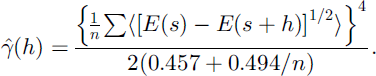
Here, h is the lag distance between two locations for which the semivariogram is calculated. The lag distance was divided into 20 classes with n point pairs, over which the summation in Equation (3) was done. We then modeled the sample semivariogram with a spherical semivariogram model plus a constant (c₀) for h ≤10 m. The model semivariogram was defined by

(4)

and characterized by its range (a), its sill variance (c) and the nugget variance (c₀). The sill variance is a measure of the intensity of the fluctuation of the variable around the slope-scale trend. The range is a measure for the distance over which E(s) is autocorrelated. The nugget is caused by measurement error and by variance in E(s) at shorter distances than the minimum measurement spacing, in our case 0.5 m. We fitted γ̄(h) to γ̂(h) using the weighted least-squares method described by Reference CressieCressie (1993).

3. Results

In the snow pit, the total snow depth was 180 cm. Within the grid, it varied between 150 and 210 cm. The upper part of the snow cover was dominated by small round grains down to a prominent layer of large buried surface-hoar crystals 58 cm below the surface (Fig. 2). The grains below the buried surface-hoar layer were primarily mixed forms. Three failures were produced by the rutschblock test (Fig. 2). The buried surface-hoar layer was the failure plane in the slab avalanche next to the slope investigated.

Fig. 2.

Snow stratigraphy and hardness profiles in the snow pit. Hardness profiles were measured with the rammsonde, the SMPand by hand (1 = fist; 2 = four fingers; 3 = one finger; 4 = pencil; 5 = knife). The depth of the hand hardness and the rammsonde penetration resistance is corrected to depth perpendicular to the snow surface. Letters in bold refer to the layers traced through the grid. Locations of failures produced by the rutschblock test are given with their score (RB). Samples A and B were taken at the upper and lower rutsch-block failure, respectively.

3.2. Layer boundaries

For all layers, the continuous profile of penetration resistance from the SMP showed a gradual change in penetration resistance as the tip moved from one layer to another (Fig. 2 and 3). Visual analysis of the SMP profiles of penetration resistance indicated that the transitions between layers spanned 1–5mm, the average being around 2 mm. Figure 3 shows how the boundaries of five layers were defined based on the microstructural information and the SMP penetration resistance profile.

Fig. 3.

Planar sections of two samples with the corresponding micropenetrometer resistance. Although there were boundaries of transition in penetration resistance between adjacent layers, it was possible to manually identify individual layers. The locations of layer boundaries for five layers are shown. The scale for SMP penetration resistance next to sample A is one-third that for sample B.

3.3. Spatial continuity of layers

To demonstrate the spatial continuity of layers, one transect through the grid in the cross-slope direction and one in the up-slope direction are shown in Figure 4. Themeasurement point where the two transects cross is indicated with arrows in the figure. Eleven layers are marked with letters a–k in the figure and traced with lines through the transects. The location of the two transect lines in the grid is shown in Figure 1. In most of the grid, the stratigraphy of the most distinctive layers was not difficult to reconstruct based on the SMP profiles. In the upper part of the grid (Fig. 4), however, individual layers were hard to follow. Yet, we were still able to trace some distinct layers through all 113 SMP profiles. Among the continuous layers were the weak layers b and j, in which the upper and lower rutschblock failure occurred, and layer f, above which the middle failure occurred (Fig.2).

Fig. 4.

SMP penetration resistance profiles measured along the two transects indicated in Figure 1. Only the upper 80 cm of the snow cover is shown. Eleven distinct layers are marked with letters a – k and traced with lines through the two transects. Arrows indicate the profile where the two transects cross.

3.4. Spatial variability of penetration resistance of layers

Layers b, f, g, i, j and k were chosen for further analysis. Layer b was split up into an upper part (b_weak) and a lower part (b_hard), which gave us seven layers to analyze. These layers were the ones that we had found in all 113 SMP profiles, and so represented the more continuous and distinct layers in the grid. The grain type and size of these layers are shown in Figure 2.

The Kolmogorov–Smirnov test for normality of the log10-transformed data gave p ≤ 0.05 for all layers. For three layers (b_weak, i and j) we found p ≤ 0.01. All calculations were therefore done for the log-transformed values, for which the mean and the coefficient of variation are shown in Table 1. Mean penetration resistance in the layers varied between 0.06 and 0.78 N.

Table 1.

Summary statistics for the log-transformed penetration resistance in the seven layers investigated

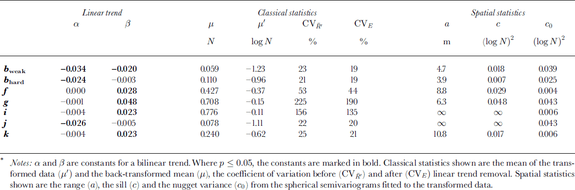
Linear spatial trends were statistically significant for all layers (Table 1). Generally, the transformed values decreased in the positive x direction (to the right) and increased in the positive y direction (uphill). Penetration resistance was generally higher in the left side and in the upper part of the grid.

The spherical models with a nugget variance are shown for representative layers in Figure 5a–d. The model semivariograms showed large variations in range, sill and nugget variance (Fig. 5e; Table 1). The infinitely large range values for layers i and j indicate that in these layers the mean penetration resistance varies over the grid, and the variance increases without bound even after removal of a linear trend.

Fig. 5.

Sample (unfilled circles) and model (lines) semivariograms for the log-transformed penetration resistance. Circles in the sample variograms are scaled in proportion to the number of measurements in each group. (a–d) show the semivariograms for layers b_weak, f, g and j, respectively, drawn to different scales. (e) shows the semivariogram models for the seven layers on the same scale. Units for the semivariance γ are (log_N2).

4. Discussion

In the SMP profiles, we could identify the same layers as found in the stratigraphic record as well as some additional layers (Fig. 2). This gave us confidence in the SMP as a useful instrument to identify layers in the snow cover, thereby supporting the results of Reference Pielmeier and SchneebeliPielmeier and Schneebeli (2003).

The identified layers were separated from the adjacent layers by boundaries of gradual transition in penetration resistance. The boundaries were around 2 mm thick. These boundaries were partly due to the length of the SMP tip: the narrow front part of the tip might be in one layer while the wider back is still in the adjacent layer. However, 60% of the penetration resistance is sensed in the widest 1.3 mm in the back of the tip due to the distribution of the surface area of the tip. Boundaries of <1mm between adjacent layers were also observed, confirming the ability of the SMP to resolve layers and boundaries down to a thickness of around 1mm, supporting the observations by Reference Pielmeier and SchneebeliPielmeier and Schneebeli (2003). This confirms our perception of layer boundaries: these cannot be sharper than a single grain diameter and are more likely to be a few diameters thick, typically ranging from 0.5 to 5 mm. The existence of such boundaries can also be seen in three-dimensional reconstructions of natural snow (e.g. Reference SchneebeliSchneebeli, 2001).

Despite these transition boundaries, we were able to identify distinct layers in the snow cover. In a study of a layer of buried surface hoar, Reference Birkeland, Kronholm, Schneebeli and PielmeierBirkeland and others (2004) found that changes in the exact location of the defined boundaries around the layer did not significantly change the mean penetration resistance of the layer. We similarly expect that the exact location of the defined boundaries for each measurement in this study is not critical for the median penetration resistance of that layer.

In the upper 80 cm of the snow cover within the grid, around 15 layers could be traced through most of the profiles. Eleven of these layers are shown in Figure 4. The seven layers chosen for further analyses were found in all 113 SMP profiles within the grid. They were some of the most distinct layers in the snow cover within the grid. Between the 15 distinct layers, at least as many non-distinct layers could be identified. These could not be traced through the snow cover within the grid. Particularly in the upper third of the grid, towards the top of the slope, less distinct layers present in the lower part of the grid could not be identified with confidence. This finding is in agreement with other studies that suggest that sites towards the top of slopes should not be chosen for representative snow-cover profiles and snow stability tests (Reference Jamieson and JohnstonJamieson and Johnston, 1993).We expect the disturbance observed in the snow cover in the upper part of the grid to be due to snow rolling down from an exposed rocky outcrop above the grid.

Apart from this disturbance, we expect the inherent variability of distinct layers on the slope to be primarily caused by wind. We can test this hypothesis with the buried surface-hoar layer: low wind speed is among other things a prerequisite for surface hoar formation (Reference Hachikubo and AkitayaHachikubo and Akitaya, 1997). After deposition, surface hoar crystals can easily be disturbed due to their fragile nature. The buried surface-hoar layer in our grid, layer j, had a low coefficient of variation, and the spatial variation was in the form of a trend with little additional spatial structure found, thus supporting our hypothesis. Layers g and i had large variations and were probably deposited under windy conditions. However, for a complete verification of our hypothesis, we need continuous weather data and simultaneous observations of layer formation. Measurements from more layers are also needed.

Previous studies of slope-scale spatial variability have focused primarily on variations in the shear strength of weak layers. A direct comparison between variations in shear strength and penetration resistance cannot be made. However, we note that Reference Jamieson and JohnstonJamieson and Johnston (2001), in a comprehensive study of shear strength variation in weak layers, report coefficients of variation of up to 66% but typically around 15%. Penetration resistance of the buried surface-hoar layer and three other layers had coefficients of variation of around 20%, that is within the range found for shear strength by Reference Jamieson and JohnstonJamieson andJohnston (2001). However, in layers g and i, the penetration resistance varied around 200%, suggesting that much higher variations in penetration resistance exist in some layers.

In terms of snow stability, the most critical weak layer in the snow cover was the buried surface-hoar layer, layer j, judged from the slab avalanche nearby. This layer had a low penetration resistance everywhere and little spatial variation. The layers that made up a part of the slab, especially layers f, g and i, had a higher spatial variation than the buried surface-hoar layer, and the penetration resistance in the layers varied over different spatial scales. More slopes need to be investigated to see if snow slabs are generally more variable than weak layers.

It is possible to calculate snow microstructural and micromechanical properties from the SMP penetration resistance signal (Reference Johnson and SchneebeliJohnson and Schneebeli, 1999). The spatial variation of these properties could provide more information about the influence of spatial variability on slab avalanche release and should be investigated further.

5. Conclusions

With a micropenetrometer, we measured some of the inherent spatial variability of penetration resistance in snow layers on an alpine snow slope. We observed that adjacent layers are separated by boundaries with a variable thickness of transition. Despite this, we could identify distinct layers based on penetration resistance. Some of these distinct layers, both hard and soft, were found in all measurements in the grid, but less distinct layers could not be identified in all measurements. The spatial variability of seven layers was analyzed. Five layers had a coefficient of variation in penetration resistance around 25%. These layers were presumably deposited during conditions with low wind speed. Two layers had coefficients of variation around 200%. These layers might have been deposited during high winds. A slope-scale trend was present in all layers. The layers showed different degrees of autocorrelation. The maximum length of autocorrelation varied from 4m to a distance longer than the size of our grid. The most critical weak layer in the grid was a layer of buried surface hoar, which was identified in all measurements. The layer had a relatively low coefficient of variation and had little spatial variation. The layers in the slab above this weak layer showed a more complex structure, with generally higher variation coefficients and different ranges from layer to layer.

The present work is a first step towards quantifying the layered character of an Alpine snow cover. Our conclusions are restricted to seven layers in the snow cover within one grid. To reach conclusions that are more general, additional layers and slopes must be studied. Future aims are to develop an algorithm that automatically identifies layers and to investigate lens-like layers, i.e. layers that are not present in all measurements. In addition, the description of vertically penetrating features such as flow paths and skier tracks, as well as investigating a possible relation between snow-cover variability and snow-slope stability, will be a challenge.