1 Introduction
Data mining is the type of analysis made possible by modern computers, which uses powerful processors to mine through large databases to reveal previously unsuspected or unquantified trends and relationships. Hastie et al. (Reference Hastie, Tibshirani and Friedman2008) provide a description of data mining and a catalogue of methodogy. In recent years, increasing computing power has made the storage and analysis of large datasets more feasible. This evolution of computing technology has a big impact on the insurance industry in particular. More and more information related to policyholders are being collected and stored in the insurers’ information systems. Whether the insurers can utilise this information collected in order to better understand the risks underwritten becomes the key to pricing, reserving and claims management. The data mining techniques can be very powerful as a method for uncovering trends or patterns that were previously hidden in these complex datasets.
Nowadays, some practicing actuaries have already started to apply data mining methods in their work. In early 2001, Senensky and Polon founded a consulting company called Claim Analytics with the objective of using data mining tools for predictive modelling to assist major insurance companies with claim scoring, pricing, reserving and fraud detection. This paper is inspired by a case study done by Senensky and Polon on prediction of return to work for group insurance claimants with long term disabilities in Reference Senensky and Polon2004. We further explore how other data mining techniques can be applied to predict duration classes of insured lives under Income Protection Insurance (IPI). Income Protection Insurance plays a significant role in maintaining the quality of life of individuals, of working age, who become unable to work due to a non-work related injury or an illness. It achieves this by providing such insured lives with a proportion of their usual salary during the time that they are unable to work. A major risk for providers of the IPI business comes from the fact that the claim duration can vary considerably for different IPI policies.
We use data mining techniques to classify claims into different sickness duration classes. This classification can help claims managers to identify the high risk policies that are predicted to have long sickness durations. It can help claim managers to optimise the allocation of available resources, and to spend time where it is most productive. The factors that are found significant in predicting sickness duration class may also provide some useful insights for reserving and pricing.
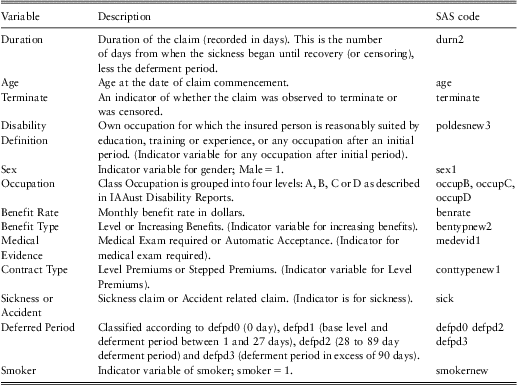
We have obtained Australian IPI claim data from the Actuaries Institute of Australia (IAAust) income protection insurance policy database, which contains comprehensive information on policyholders who have purchased insurance from the main Australian providers of IPI. Data are recorded for each policyholder based on the information provided in the insurance proposal form. The data were previously analysed by Pitt (Reference Pitt2007) and contain all claim records beginning in calendar year 1995. The total number of claim records in respect of calendar year 1995 is 8863. These claims were followed until termination or the end of calendar year 1998, whichever occurred first. Available information provided in the data set includes the duration of each policyholder's claim, the age of the claimant at the onset of disability, the definition of disability used in assessing whether the policyholder is eligible for a benefit under the policy, the gender of the policyholder, the occupation class of the policyholder (classified into four levels, see the Report of the IAAust Disability Committee, 1997), the rate of benefit payable monthly, the type of benefits payable (increasing in line with inflation or level), the smoker status of the insured life and the deferment period specified in the insurance contract. Table 1 provides a summary of the potential rating factors recorded for each of these claimants along with the coded SAS variable name and a brief description of the variable.
IPI Data Fields.

We develop a classification scale for insured lives, where 1 indicates extremely short claim duration class and 10 indicates a very long claim duration class. Being able to identify groups of policyholders with similar risks can help actuaries to better understand the risk portfolios underwritten. We attempt to apply and evaluate several data mining methods to predict claim duration class using various rating factors. Results from fitting different prediction models are compared based on two different loss functions.
We then suggest using principal components analysis to better understand the relationship between various rating factors and how they impact claim duration class. We also discuss and compare how different variable combining techniques can be used to select and weight available variables used in the prediction models. While we have some understanding of the level of claim termination rates from existing industry tables and other industry level studies (e.g. CMI 12 1991 and Ling et al. Reference Ling, Waters and Wilkie2010), this paper will provide a new outlook on IPI data classifications formulated using modern statistical methods that have not previously been used to advance our understanding of this area in Australia. We hope that this paper will appeal not just to researchers but also to actuarial practitioners in the insurance industry. All models are applied using SAS functions and more details can be found in Liu (Reference Liu2013).
The rest of the paper is organised as follows. Section 2 presents a brief discussion of the data mining models that are used to predict claim duration classes of insured lives. Section 3 demonstrates how principal components analysis and different variable combining techniques can be used to better understand rating factors that drive claim durations. Section 4 presents and compares the results of fitting different data mining models with various variable selection and weighting techniques and Section 5 concludes the paper.
2 Data Mining Prediction Models
We aim to provide a fast, objective method of scoring claims into different portfolios with homogeneous risks. First of all, we define claim duration as the time difference between claim termination and the date of claim onset. We classify the claim durations T into 10 different classes of duration with approximately 10% of available data in each class, ranging from the shortest claim duration class G = 1 to the longest claim duration class G = 10. The goal is to use various policyholders’ information known to the insurers to group the policies into 10 different duration portfolios. The prediction model assigns each new claim a score from 1 to 10. The higher the score, the longer the predicted claim duration.
An alternative approach is to classify data with classes of equal length. The advantage of this approach is the interpretability of a misclassification in terms of the number of days. The disadvantage, relative to our equal proportion bins, is the lack of data in particular bins due to the positive skewness in the distribution of expected claim durations. This unbalanced distribution of data across bins makes classification and statistical learning more difficult to achieve. We have therefore opted to use bins containing equal volumes of data.
We apply six different data mining techniques to create our prediction model namely Linear Regression of an Indicator Matrix, Linear Discriminant Analysis (LDA), Quadratic Discriminant Analysis (QDA), K-Nearest Neighbour (KNN), Log-logistic Regression and Ordered Log-logistic Regression. Even though we explain some important mathematical details, we emphasise the methods and their conceptual underpinnings more. For more information on model specifications and associated mathematical details see Hastie et al. (Reference Hastie, Tibshirani and Friedman2008).
2.1 Linear regression of an indicator matrix
We start off with this most straight forward and widely used regression model. For our analysis, the response variable duration class is denoted by G, which can take values 1, 2,…, 10. This quantitative outcome is known as a categorical response. By using linear regression, we assume there is no explicit ordering in the classes. We record the predictors using a vector X representing the p predictor variables which include age, gender, and occupation category amongst others. Components of X are denoted Xj, j = 1, 2,…, p. Using N to denote the number of observations, the entire set of the predictors is a set of N input p-vectors Xi, i = 1,…, N recorded in an N × p matrix X. An indicator variable is used to code each of the response categories. Since G has 10 classes, there will be 10 such indicators Yk, k = 1,…, 10 with Yk = 1 if G = k else 0. Often it is convenient to include the constant variable 1 in X, and write the linear model as
 $$\hat{\bf Y}\, = \,{{\bf X}^\top} \hat{\bf B},$$
where  $$$\hat{\bf B} $$$
denotes the estimated coefficient matrix. Using the least squares method, the fit is given by
 $$\hat{\bf B}\,{\rm{ = }}\,{{{\rm{(}}{{\bf X}^ \top } \bf X{\rm{)}}}^{{\rm{ - 1}}}} {{\bf X}^ \top } \bf Y{\rm{.}}$$
More details can be found in Myers (Reference Myers2000). A new observation with input  $$$ {{x}^\top} \, = \,({{x}_1}, \ldots, {{x}_p}) $$$
is classified as follows:
• compute the fitted output
 $$$ \hat{f}{{(x)}^ \top } \, = \,(1,{{x}^ \top } )\hat{B} $$$
, a 10 vector;
• identify the largest component and classify accordingly:

 $$\hat{G}(x)\, = \,{\rm{argmax}}{{}_{k\, \in \,G}}\,{{\hat{f}}_k}(x),$$
where  $$$ {{\hat{f}}_k}(x) $$$
is the fitted linear model for the kth indicator response variable.
Hastie et al. (Reference Hastie, Tibshirani and Friedman2008) point out there is a serious masking problem with the regression approach when the number of classes K ≥ 3, especially prevalent when K is large. Because of the rigid nature of the regression model, classes can be masked by others. We therefore look at Linear Discriminant Analysis (LDA) in the next section, which can prevent this masking problem.
2.2 Linear discriminant analysis
Discriminant analysis is a classic method of classification that has stood the test of time. It was originally developed in 1936 by Reference FisherFisher. Discriminant analysis often produces models whose accuracy approaches and occasionally exceeds more complex modern methods. Discriminant analysis can only be used for classification problems, not for regression. That is, the target variable must be categorical, but may have two or more categories. Suppose that we model the class density for each observed predictor set using a multivariate Gaussian distribution,
 $${{f}_k}(x)\, = \,\frac{1}{{2{{\pi }^{p/2}} |{{\brSigma }_k}{{|}^{1/2}} }}{\exp }^{{\rm{ - }}1/2(x\,{\rm{ - }}\,{{\mu }_k}{{)}^ \top } \brSigma _{k}^{{{\rm{ - }}1}} (x\,{\rm{ - }}\,{{\mu }_k})}, \ {\rm{for}} \ \,k\, \ {\rm{in}} \ 1,2, \ldots, 10,$$
where p is the number of predictors available, x is the predicting vector with each element representing information such as age, gender, and occupation category etc, μ and Σk are the mean vector and variance matrices of the multivariate Gaussian distribution. We are aware of the fact that we have some predictors here that are categorical, which technically violates the normality assumption. However, Manly (1986) pointed out that violation of the normality assumption does not render discriminant analysis a waste of time. He states that discriminant analysis may well turn out excellent even on data from non-normal distributions. This should also apply in cases where the vast majority of the variables are categorical. We therefore decide to look at both linear discriminant analysis (LDA) and quadratic discriminant analysis (QDA). We will demonstrate in the results section that even though these two models do not perform as well as methods such as k-nearest neighbour, there is still some predictability evident when we look at the misclassification plots.
Let us denote πk as the prior probability for class k, with  $$$ \mathop{\sum}\nolimits_{k\, = \,1}^{10} {{\pi }_k}\, = \,1 $$$
. The predicted outcome is classified based on the decision function
 $$G(x)\, = \,{\rm{argmax}}{{ }_k}{{\delta }_{k(x)}},$$
where δk (x ) are the conditional probabilities of being classified as class k given a set of predictors x:
 $${{\delta }_k}(x)\, = \,{\rm{log}}\,\left\{ {{\rm{Pr}} \ (G\, = \,k|X\, = \,x)} \right\}\, = \,{{x}^ \top } {{\brSigma }^{{\rm{ - }}1}} {{\mu }_k}{\rm{ - }}\frac{1}{2}\mu _{k}^{\top} {{\brSigma }^{{\rm{ - }}1}} {{\mu }_k}\, + \,{\rm{log}} {{\pi }_k}.$$
More details can be found in Manly (1986). In practice, the parameters μ and Σ in the Gaussian distributions and the prior probability πk are not known and therefore we need to estimate them using our training data. The algorithm is as follows:
• Estimate the prior probability for each class
$$$ \hat{\pi }\, = \,{{N}_k}/N $$$
, where Nk is the number of observations in class k and N is the total observations in the training set.• Estimate the mean for each class:
$$$ {{\hat{\mu }}_k}\, = \,{{\rSigma }_{{{y}_i}\, = \,k}}{{x}_i}/{{N}_k} $$$
,
$$$ k\, = \,1,2, \ldots, 10 $$$
.• Estimate the common covariance matrix
$$$ \hat{\brSigma }\, = \,\rSigma _{{k\, = \,1}}^{{10}} {{\rSigma }_{{{y}_i}\, = \,k}}({{x}_i}\,{\rm{ - }}\,{{\hat{\mu }}_k})({{x}_i}\,{\rm{ - }}\,{{\hat{\mu }}_k}{{)}^{\rm \top}} /(N\,{\rm{ - }}\,10) $$$
.



With two classes there is a simple correspondence between linear discriminant analysis and classification by linear regression introduced in earlier section. Hastie et al. (Reference Hastie, Tibshirani and Friedman2008) showed that with more than two classes, LDA is not the same as linear regression of the class indicator matrix, and it avoids the masking problems associated with that approach.
2.3 Quadratic discriminant analysis
Quadratic Discriminant Analysis (QDA) is similar to LDA, except that separate covariance matrices Σk must be estimated for each class of outcomes. If Σk are not assumed to be the same for all 10 classes, the decision boundary is a quadratic function of the predictors x. Applying similar logic to Equation (1) , we get the quadratic discriminant functions,
 $${{\delta }_k}(x)\, = \,{\rm{ - }}\frac{1}{2} {\rm{log}} \ |{{\brSigma }_k}|{\rm{ - }}\frac{1}{2}{{(x\,{\rm{ - }}\,{{\mu }_k})}^ \top } \brSigma _{k}^{{{\rm{ - }}1}} (x\,{\rm{ - }}\,{{\mu }_k})\, + \,{\rm{log}} {{\pi }_k}\,\,{\rm{for}}\,\,k\, = \,1,2, \ldots, 10.$$
The decision boundary between each pair of classes k and l is described by a quadratic equation  $$$\{ x\,:\,{{\delta }_k}(x)\, = \,{{\delta }_l}(x)\} $$$
.
Michie et al. (Reference Michie, Spiegelhalter and Taylor1994) demonstrated that both LDA and QDA perform well on a large and diverse set of classification tasks. Hastie et al. (Reference Hastie, Tibshirani and Friedman2008) suggest that the reason why LDA and QDA have such good performance records is not because the data are approximately Gaussian, nor because the covariances are approximately equal for LDA. Instead, they suggest it is because the data can only support simple decision boundaries such as linear or quadratic, and the estimates provided via the Gaussian models are stable. That is, these models may have relatively high bias, but can be estimated with much lower variance than more complicated alternatives.
2.4 Multinomial logistic regression
Logistic regression is another type of regression analysis used for predicting categorical outcomes based on one or more predictor variables. For categorical outcomes it is inappropriate to use linear regression because the linear regression model can generate any real number ranging from negative infinity to positive infinity, whereas our categorical outcome can only take on discrete values 1, 2,…, 10. Instead of equating the expected value of the dependent variable to a linear combination of independent variables and their corresponding parameters as with linear regression, logistic regression models equate the linear component to the logit function of the probability of a given outcome of the dependent variable. For our analysis, we have 10 discrete duration classes for the dependent variable. We will consider the 10th category to be the omitted or baseline category, where logits of the first 9 categories are constructed with the baseline category in the denominator. The model has the form
 $${\rm{log}} \ \frac{{ \ {\rm{Pr}} \ (G\, = \,k|X\, = \,x)}}{{ \ {\rm{Pr}} \ (G\, = \,10|X\, = \,x)}}\, = \,{{\alpha }_k}\, + \,\beta _{k}^{ \top } x,\,\,{\rm{for}} \ k \ {\rm{in}} \ 1,2, \ldots, 9,$$
where x still denotes the observed predicting vector  $$$ {{x}^ \top } \, = \,({{x}_1},{{x}_2}, \ldots, {{x}_p}) $$$
, and αk and βk are the intercepts and regression coefficient vector respectively. Although we use class 10 as the denominator in the odds-ratios, the choice of denominator is arbitrary. Solving for
 $$$ {\rm{Pr}}\:(G\, = \,k|X\, = \,x) $$$
, we have
 $$ \ {\rm{Pr}} \ (G\, = \,k|X\, = \,x)\, = \,\frac{{ \ {\rm{exp}} ({{\alpha }_k}\, + \,\beta _{k}^{ \top } x)}}{{1\, + \,\mathop{\sum}\limits_{l\, = \,1}^9 \ {\rm{exp}} ({{\alpha }_l}\, + \,\beta _{l}^{ \top } x)}}, \ {\rm{for}} \ k\, = \,1,2, \ldots, 9$$
 $${\rm{Pr}} \ (G\, = \,10|X\, = \,x)\, = \,\frac{1}{{1\, + \,\mathop{\sum}\limits_{l\, = \,1}^9 \ {\rm{exp}} ({{\alpha }_l}\, + \,\beta _{l}^{ \top } x)}}.$$
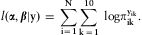
The probabilities of being classified in each of the 10 classes obviously sum to one. Denote G to be the duration class random variable, which can take one of 10 possible values. For a given set of predictors x on N observations, G can be considered a column vector of N multinomial random variables Gi. Let Y be a N × 10 indicator response matrix with Yik = 1 if Gi = k else 0. π is a matrix of the same dimension as Y where each element πik is the probability of observing the kth value of the dependent variable G for any given observation in the ith row. Thus, the likelihood function is
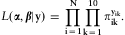 $$L(\bialpha, \bibeta |\bf y)\, = \,\prod\limits_{i\, = \,1}^N \prod\limits_{k\, = \,1}^{10} \pi _{{ik}}^{{{{y}_{ik}}}} .$$
The log-likelihood is
 $$l(\bialpha, \bibeta |\bf y)\, = \,\mathop{\sum}\limits_{i\, = \,1}^N \mathop{\sum}\limits_{k\, = \,1}^{10} \ {\rm{log}} \pi _{{ik}}^{{{{y}_{ik}}}} .$$
Unlike linear regression with normally distributed residuals, there is no closed-form expression for the coefficient values that maximise the likelihood function, however we can use an iterative process such as Newton's method instead.
By fitting a multinomial logistic model, we ignore any ordering in the values of the duration class. We fit the same model if the duration class is as short as 1 or as long as 10. The advantage of the logistic regression model is that we estimate coefficients that capture differences between all possible pairs of duration classes. However, for our analysis, the predicted outcome is clearly ordered from short duration to long duration, therefore we also look at ordered logistic regression in the next section.
2.5 Ordered logistic regression model
Our dependent variable duration class is ordinal, that is, it is ranked from the shortest duration class to the longest duration class. We consider a model that incorporates the ordinal nature of our dependent variable. The ordered logistic regression model, also known as the proportional odds model, can be applied here. Ordered logistic regression models cumulative probability. For our analysis, the event of interest is observing a particular duration class or less. We model the following odds ratios (McCullagh, Reference McCullagh1980):
 $${\rm{log}} \ \frac{{ \ {\rm{Pr}} \ (G\,\leq \,k|X\, = \,x)}}{{1{\rm{ - }} \ {\rm{Pr}} \ (G\,\leq \,k|X\, = \,x)}}\, = \,{{\alpha }_k}\,{\rm{ - }}\,{{\beta }^ \top } x,\,{\rm{for}}\,k\, = \,1, \ldots, 9,$$
where all the parameters and vectors are defined in the same way as for the logistic model defined in Section 2.4. The last category does not have an odds associated with it since the probability of being classified into a duration group that is less than or equal to 10 is 1. Notice the negative sign of the β coefficients in the linear predictors above. This ensures that larger coefficients indicate an association with a longer duration group. For a continuous variable, a positive coefficient tells us that as the values of the variable increase, the likelihood of being in a longer duration group increases. An association with longer duration class means smaller cumulative probabilities for shorter duration class, since they are less likely to occur. The model is called the proportional odds model because the log of cumulative odds ratio of making the same responses at different x-points is proportional to the distance of the points,
 $${\rm{log}}\,\left\{ {\frac{{ \ {\rm{Pr}} \ (G\,\leq \,k|X\, = \,{{x}_1})}}{{1\,{\rm{ - }}\,{\rm{Pr}} \ (G\,\leq \,k|X\, = \,{{x}_1})}}\,\times \,\frac{{1\,{\rm{ - }}\,{\rm{Pr}} \ (G\,\leq \,k|X\, = \,{{x}_2})}}{{{\rm{Pr}} \ (G\,\leq \,k|X\, = \,{{x}_2})}}} \right\}\, = \,{{\beta }^ \top } ({{x}_2}\,{\rm{ - }}\,{{x}_1}).$$
Maximum likelihood estimation is used to estimate the parameters αk and β. Using the relationship equation  $$${\rm{Pr}}\:(G\, = \,k|X\, = \,x)\, = \,{\rm{Pr}}\:(G\,\leq \,k|X\, = \,x)\, - \,{\rm{Pr}}\:(G\,\leq \,(k\,{\rm{ - }}\,1)|X\, = \,x)$$$
, the likelihood function can be derived in a similar way as for the logistic regression model.
The model constrains the classified group curves to have the same shape as shown in Equation (2), and therefore we cannot fit it by fitting separate logit models for each group as for multinomial logistic regression model introduced in Section 2.4. We must maximise the multinomial likelihood subject to a constraint. The model only applies to data that meet the proportional odds assumption, that is the relationship between any two pairs of outcome groups is statistically the same.
2.6 Nearest-neighbour classifier
The k-Nearest-Neighbour Method is essentially a model-free method for classification and pattern recognition. Because it is highly unstructured, it typically is not useful for understanding the nature of the relationship between the predictors and class outcome. However, as a black box prediction engine, it can be very effective, and is often among the best performers in real data problems. The k-nearest classifiers are memory-based, given a query point x 0, we find the k training points  $$$ {{x}_{(r)}},r\, = \,1, \ldots, k $$$
closest in distance to x 0, and then classify using majority vote among the k neighbours. Ties are broken at random. For simplicity we will assume that the features are real-valued, and we use Euclidean distance in the feature space:
 $${{d}_i}\, = \,|{{x}_i}\, - \,{{x}_0}|.$$
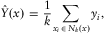
The k-nearest neighbour fit for duration class  $$$ \hat{Y} $$$
is defined as follows:
 $$\hat{Y}(x)\, = \,\frac{1}{k}\mathop{\sum}\limits_{{{x}_i}\, \in \,{{N}_k}(x)} {{y}_i},$$
where Nk(x) is the neighbourhood of x defined by the k closest points xi in the training sample, and we average the corresponding observed class indicator outcomes. We then find the largest fitted value among  $$$ {{\hat{Y}}_1}, \ldots, {{\hat{Y}}_{10}} $$$
, and assign to class
 $$$ \hat{G} $$$
accordingly. Statistical decision theory can provide a framework for developing the model. Since our output is a categorical variable G, Hastie et al. (Reference Hastie, Tibshirani and Friedman2008) has proved that the solution to minimising expected prediction error
 $$$ E[L(G,\hat{G}(X))] $$$
is simply
 $$ \hat{G}(X)\, = \,{\rm{maxPr}}(g|X\, = \,x). $$
This solution is known as the Bayes classifier, and it tells us that we classify to the most probable class, using the conditional discrete distribution  $$$ {\rm{Pr}}(G|X) $$$
. The error rate of the Bayes classifier is called the Bayes rate. Another way of representing the Bayes classifier is
 $$$ E({{Y}_k}|X)\, = \,{\rm{Pr}}(G\, = \,{{G}_k}|X) $$$
. This is the dummy-variable regression procedure, followed by classification to the largest fitted value. It is not hard to understand that for k-nearest-neighbour fits, the error on the training data should be approximately an increasing function of k. The bias of the 1-nearest-neighbour estimate is often low because it uses only the training point closest to the query point, but the variance is high. A famous result of Cover and Hart (Reference Cover and Hart1967) shows that asymptotically the error rate of the 1-nearest-neighbour classifier is never more than twice the Bayes rate. We would need an independent test set for comparing the different methods. The k-Nearest-Neighbour Method can be applied in SAS using PROC DISCRIM and a nonparametric method (using option METHOD = NPAR K=).
Unlike the least squares methods, the k-nearest-neighbour procedures do not appear to rely on any stringent assumptions about the underlying data. However, any particular subregion positions of the decision boundary can depend on a handful of input points and can thus too specific to the data and unstable, resulting in high variance and low bias. It seems that with a reasonably large set of training data, we could always approximate the theoretically optimal conditional expectation by k-nearest-neighbour averaging, since we should be able to find a fairly large neighbourhood of observations close to any x and average them. However this approach breaks down in high dimensions. It can be shown that, in a high dimensional space, in order to capture a small percentage of the data to form a local average, we must cover a big range of each input variable. Such a neighbourhood is no longer “local”. This is commonly known as the curse of dimensionality (Bellman, Reference Bellman1961).
2.7 Model assessment
We discuss the appropriate performance assessment criteria to use in order to compare models. A loss function approach is often used to evaluate the accuracy of a categorical predictor  $$$ \hat{G} $$$
. Let
 $$$ L(G;\hat{G}) $$$
denote the loss incurred when
 $$$ \hat{G} $$$
is used to predict a random variable G. A loss function L(.) usually satisfies the following conditions: it is bounded below by 0 and attains 0 when correct prediction is made, i.e.
 $$$ \hat{G}\, = \,G $$$
; For a categorical variable G, a widely used loss function is:
 $$L(G;\hat{G})\, = \,I(G\, \ne \,\hat{G})$$
where  $$$ I(.) $$$
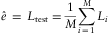
is the indicator function. For a set of test data, the prediction error e can be estimated via
 $$\hat{e}\, = \,{{L}_{ {\rm{test}} }} = \frac{1}{M}\mathop{\sum}\limits_{i\, = \,1}^M {{L}_i}$$
where M is the number of test data, and Li is a indicator variable for misclassification. One disadvantage of this loss function is that it does not measure how serious is the misclassification. In other words, misclassifying a G = 1 observation as G = 10 has the same contribution to prediction error as misclassifying it to G = 2. We prefer the loss function to increase as the distance between G and  $$$ \hat{G} $$$
increases. A more appropriate loss function for our analysis is therefore
 $$L(G;\hat{G})\, = \,|G\,{\rm{ - }}\,\hat{G}|,$$
and L is the loss distance between the number of class difference between the test observation and the predicted class outcome.
3 Variable Selection
3.1 Stepwise Regression Technique
We mentioned in earlier sections that some data mining models such as k-nearest neighbour do not provide much useful information on the relationship between the predictors and the class outcome. We can use methods such as forward selection or backward elimination to select variables (see for example, Hocking, Reference Hocking1976; Wilkinson and Dallal, Reference Wilkinson and Dallal1981). Forward selection involves starting with no variables in the model, testing the addition of each variable using a chosen model comparison criterion, adding the variable that improves the model the most, and repeating this process until none improves the model. Backward elimination involves starting with all candidate variables, testing the deletion of each variable using a chosen model comparison criterion, deleting the variable that improves the model the most by being deleted, and repeating this process until no further improvement is possible. We chose to use the backward elimination technique to identify the significant variables for explaining claim durations. Eight variables are found to be significant across all data mining methods. They are age at the date of commencement (age), indicator variable (terminate) to indicate whether the claim was observed to terminate or was censored, indicator variable for male (sex1), monthly benefit rate in dollars (benrate), indicator for medical exam required (medevid1), indicator for sickness claim or accident related claim (sick), indicator variable for deferred period 0 (defpd0) and indicator variable for deferred period in excess of 90 days (defpd3). Furthermore, we also explore using principal components analysis and weighted combination models as two alternative ways of selecting and weighting available variables. We compare the results from applying the various variable selection methods and discuss the relative merits of these three methods.
3.2 Principal Components Analysis Model
The technique of principal components analysis was first described by Karl Pearson (Reference Pearson1901), although he did not propose a practical method of calculation for more than two or three variables. Hotelling (Reference Hotelling1933) described the computing methods. The object of the analysis is to take p variables X 1, X 2,…, Xp and find combinations of these to produce components Z 1, Z 2,…, Zp that are uncorrelated. Since Z 1, Z 2,…, Zp are uncorrelated, it means they measure different dimensions in the data. The components are also ordered so that Z 1 displays the largest amount of variation in the response, Z 2 displays the second largest amount of variation, and so on. We aim to explain the variation in the data set using as few Z variables with variances that are not negligible. If a smaller number of Z variables can account for the variation in the p original X variables, we can achieve some degree of economy without worrying about which of the original X variables are correlated or significant for the model under consideration. The method is also useful if we think there is a good deal of redundancy in the original variables, with most of them measuring similar things. The principal components algorithm is as follows:
• Standardise X 1,…, Xn to have zero means and unit variances.
• Compute the correlation matrix
$$$ {\bf C}\, = \,\frac{1}{n}\mathop{\sum}\nolimits_{i\, = \,1}^n ({{X}_i}\,{\rm{ - }}\,\bar{X}){{({{X}_i}\,{\rm{ - }}\,\bar{X})}^ \top } $$$
for the original variables. This is a correlation matrix because Xi are standardised already.• Compute the variances of the principal components as the eigenvalues of the matrix C. Assuming that the eigenvalues are ordered as
$$$ {{{\rm{\rlambda }}}_1}\,\geq \,{{{\rm{\rlambda }}}_2}\,\geq \, \ldots \geq \,{{{\rm{\rlambda }}}_p}\,\geq \,0 $$$
, then λi corresponds to the ith principal component. Find eigenvalues:
$$$ {{{\rm{\rlambda }}}_1},\,{{{\rm{\rlambda }}}_2}, \ldots, \,{{{\rm{\rlambda }}}_p} $$$
and the corresponding eigenvectors a 1, a 2,…, ap. The coefficients of the ith principal component are then given by ai while λi is its variance.• Discard any components that only account for a small proportion of the variation in the response.



3.3 Principal Components Analysis Results
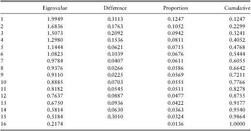
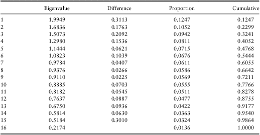
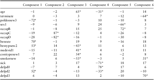
There are a total of 16 variables available that have possible impact on claim duration. It can be argued as to how many components to choose is appropriate. One rule is to use the mineigen criterion, which states that only components with eigenvalues above 1 should be retained. Components with an eigenvalue of less than 1 account for less variance than did the original standardised variable, and so are of little use. In Table 2, the first six principal components have eigenvalues over 1. We can use these six principal components for claim duration class prediction later on. Due to the dropping of the less important components, the sum of these six components can only explain a total variance of 8.71. This is also called the final communality estimate, which is of course less than total variance 16 of the original correlation matrix. Notice that the six most significant components account for around 54% of the total variance in the original correlation matrix. We will later on see in the Results section that if we only use these six most significant extracted components as predictors in the data mining model, we will not get as good predictability as using all available variables due to the information loss.
Eigenvalues of the Correlation Matrix.
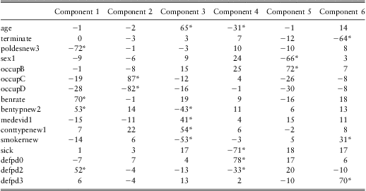
We can normally get some useful insights on the rating factors by looking at the factor pattern output, which is often referred to as the factor loading matrix in principal components analysis. The elements in the loading matrix are called factor loadings. There are at least two ways we can interpret these factor loadings. First, we can use this table to express the observed variables as functions of the extracted components. Each row of the factor loadings tells us the linear combination of the component scores that would yield the expected value of the associated variable. Second, we can interpret each loading as a correlation between an observed variable and a component, provided that the factor solution is an orthogonal one, that is, components are uncorrelated, such as the current initial factor solution. Hence, the factor loadings indicate how strongly the variables and the components are related. Values greater than 0.30122 are flagged by an *, which means the corresponding components have the largest loadings on these variables. In Table 3, the first component labelled component 1 is highly correlated with poldesnew3 and benrate, but in opposite directions. Poldesnew3 is an indicator variable for any occupation disability definition. Any occupation means an income payout occurs if by reason of illness, accident or injury the insured is unable to perform any work at all. Own Occupation definition means an income payout occurs if by reason of illness, accident or injury the insured live is unable to perform his/her normal own occupation that the insured person is reasonably suited by education, training or experience. The data show that higher benefit rate and own occupation tend to have a large positive impact on component 1. We can therefore interpret component 1 as a score for the degree of professionalism. A high degree of professionalism tends to be associated with high salary and therefore a higher benefit rate. It is intuitive that people with a highly professional occupation will generally take out cover for own occupation rather than any occupation. It is quite obvious that component 2 identifies occupation class C rather than occupation class D. Component 6 identifies claims with long deferred period (defpd3 is 1) that tend to be censored. Similarly, component 4 captures claims due to sickness, which tend to have a short deferred period (deferred period being 0).
Rotated Factor Pattern.
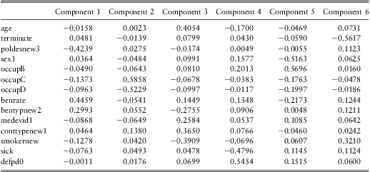
In Table 4, each component is expressed as a linear combination of the standardised observed variables. For example, the first principal component is computed as:
Standardised Scoring Coefficients.
 $$\matrix{ {{\rm{ - 0}}{\rm{.0158}}\,{\rm{\ast}}\,{\rm{age}}\,{\rm{ + }}\,{\rm{0}}{\rm{.0481}}\,{\rm{\ast}}\,{\rm{terminate}}\,{\rm{ - }}\,{\rm{0}}{\rm{.4239}}\,{\rm{\ast}}\,{\rm{poldesnew3}}\,{\rm{ + }}\,{\rm{0}}{\rm{.0364}}\,{\rm{\ast}}\,{\rm{sex1}}} \hfill \cr {{\rm{ - 0}}{\rm{.0490}}\,{\rm{\ast}}\,{\rm{occupB}}\,{\rm{ - }}\,{\rm{0}}{\rm{.1373}}\,{\rm{\ast}}\,{\rm{occupC}}\,{\rm{ - }}\,{\rm{0}}{\rm{.0963}}\,{\rm{\ast}}\,{\rm{occupD}}\,{\rm{ + }}\,{\rm{0}}{\rm{.4459}}\,{\rm{\ast}}\,{\rm{benrate}}} \hfill \cr {{\rm{ + 0}}{\rm{.2993}}\,{\rm{\ast}}\,{\rm{bentypnew2}}\,{\rm{ - }}\,{\rm{0}}{\rm{.0868}}\,{\rm{\ast}}\,{\rm{medevid1}}\,{\rm{ + }}\,{\rm{0}}{\rm{.0464}}\,{\rm{\ast}}\,{\rm{conttypenew1}}} \hfill \cr {{\rm{ - 0}}{\rm{.1278}}\,{\rm{\ast}}\,{\rm{smokernew}}\,{\rm{ - }}\,{\rm{0}}{\rm{.0763}}\,{\rm{\ast}}\,{\rm{sick}}\,{\rm{ - }}\,{\rm{0}}{\rm{.0011}}\,{\rm{\ast}}\,{\rm{defpd0}}{\rm{.}}}\hfill $$
Notice that, when applying this formula we must use the standardised observed variables (with means 0 and standard deviations 1), but not the raw data. Standardisation does not apply to categorical variables. We can then apply each data mining methods using these component scores as predictors. Results are provided and compared with other variable selection methods later on in Section 4.
3.4 Combination Prediction
Combination forecast is a technique that has been adopted by economics and finance researchers to forecast future stock returns. As pointed out in the seminal paper by Bates and Granger (Reference Bates and Granger1969), combinations of individual forecasts can outperform the individual forecasts themselves. Forecast combination has recently received renewed attention in the macroeconomic forecasting literature with respect to forecasting inflation and real output growth (e.g., Stock and Watson Reference Stock and Watson2004). We explore the combinations of individual forecast idea and apply it to the out-of-sample class prediction. Suppose there are N observations in the training data with p predicting variables available. First of all, for each observation i in the training data, we apply the data mining technique using each of the individual variables to get p estimated class predictors  $$$ {{\hat{G}}_j} $$$
for j = 1,…, p. Then for variable j, we calculate estimated weight Wj as the reciprocal of the loss value Lj defined by Equation (4),
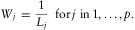 $${{W}_j}\, = \,\frac{1}{{{{L}_j}}}\, \ {\rm{for}}\,j\,\,{\rm{in}}\,1, \ldots, p.$$
The higher the loss value, the smaller weight we wish to place on that variable. The next step is to calculate the average weight  $$$ {{\bar{W}}_j} $$$
for variable j based on the N observations in the training data,
 $${{\bar{W}}_j}\, = \,\frac{1}{N}\mathop{\sum}\limits_{i\, = \,1}^N {{W}_j};$$
The estimated combination predictor  $$$ \hat{G} $$$
is taken to be the weighted average of the p individual estimated predictors based on the following equation:
 $$\hat{G}\, = \,\mathop{\sum}\limits_{j\, = \,1}^p {{\bar{W}}_j}\,\ast\,{{\hat{G}}_j}$$
where  $$$ {{\hat{G}}_j} $$$
is the predicted class using one of the data mining techniques with an individual variable j, and
 $$$ {{\bar{W}}_j} $$$
is the ex ante combining weight which is the average weight used for that particular individual prediction for the training observations. We are going to refer this method as weighted combination prediction method in later sections. Table 5 provides
 $$$ {{\bar{W}}_j} $$$
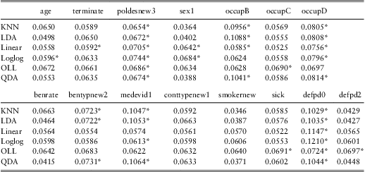
results for j in 1,…, p based on different data mining methods. We flag the six variables assigned the largest weights by * to indicate the variables that are found most significant under different data mining models. Own occupation definition (poldesnew3), Occupation class D indicator (occupD), and deferred period 0 indicator (defpd0) are among the six most significant variables across all models considered. If we compare this finding with the results found by principal components analysis in Table 3, it is interesting to see that the same variables were found to be highly correlated to the most significant components. Therefore the two methods provide fairly consistent results in terms of identifying variables that are significant.
Weights Table.
Rapach et al. (Reference Rapach, Strauss and Zhou2010) also explained two other more simple combining methods for combination forecast. The methods only differ in how the weights are determined. One of them uses simple averaging mean weight. The mean combination prediction sets Wj = 1/p, for j = 1,…, p. Therefore each individual variable predictor gets the same weight when combined together. The other method is called the trimmed mean combination forecast, which sets Wj = 0 for the individual prediction with the smallest and largest value and Wj = 1/(p−2) for the remaining individual prediction. Note that variable weights are applied individually. With relatively low collinearity between predictors we find this to be a suitable approach. An alternative approach would be to determine weights taking into account the effect of other predictor. We will apply the data mining models using all of the above mentioned variable combining methods to predict duration classes and compare their performances in the next section.
4 Data Mining Prediction Model Results
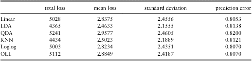
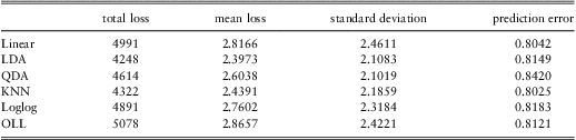
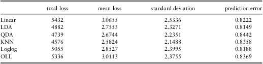
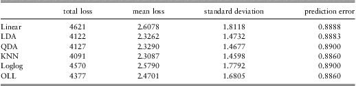
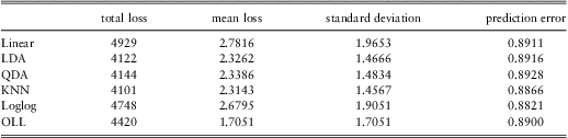
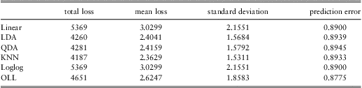
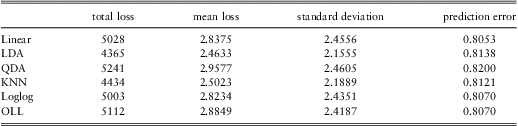
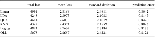
In order to build and test the model, we randomly divide the data into training and test sets according to the ratio of 80% to 20%. Data mining models are applied to the training data and a prediction model is constructed. As the test data are not used in the training of a model, they provide an independent way to evaluate the model. The test data are also used to compare and rank various models considered. For each data mining method, we obtain six sets of results. Firstly, we apply the data mining methods with all 16 available variables to do out-of-sample duration class prediction. Secondly, we apply the stepwise regression variable selection technique to reduce the number of variables used in explaining claim durations. We then apply principal components analysis to extract a few significant components that explain most variation in the variables and apply the data mining techniques using the principal components found. The last three approaches we adopt are the weighted combination prediction, the mean combination prediction, and the trimmed mean combination prediction. We apply the data mining method using each individual variable and then use these three different combining methods to predict claim class for test data.
Data Mining Results with All Variables.
Data Mining Results with Reduced Variables.
Data Mining Results with principal Components.
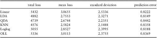
Data Mining Results with Weighted Combination Prediction.
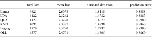
Data Mining Results with Mean Combination Prediction.
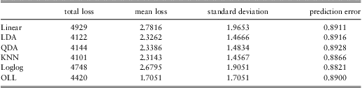
Data Mining Results with Trimmed Mean Combination Prediction.
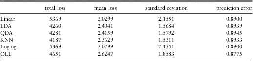
Table 6 to Table 11 provide the results on the prediction power of each data mining method. Total loss is defined as the total number of misclassifications based on the test data using the modified loss function defined by Equation (4). The average number of misclassifications together with the standard error of the misclassifications are also given. Notice that, these are all based on the modified loss function defined by Equation (4). If we define the loss function using Equation (3), it would result in very high prediction error over 80%, which overlooks the true prediction power of data mining. The predictive ability of data mining methods is clearly evident in the plot for misclassification. In Figure 1 to Figure 6, it is demonstrated that for every data mining method with every variable selection approach, there is a clear decreasing trend of policy numbers as the number of misclassifications increases. This suggests that even though the data mining methods cannot get the duration class prediction exactly right, most of the predicted outcomes are close to what we expect. This predictability can only be detected if we use the loss function defined by Equation (4).
Misclassification plot Using Linear Regression Model.
Misclassification plot Using Linear Discriminant Model.
Misclassification plot Using Quadratic Discriminant Model.
Misclassification plot Using K-nearest Neighbour Model.
Misclassification plot Using Logistic Model.
Misclassification plot Using Ordered Logistic Model.
Figure 7 provides the total loss plots for different data mining models together with various variable selection methods. It is a good way to compare across different data mining models or to compare the variable selection methods we have used. There are a few interesting findings based on Figure 7.
Total Loss on Different Data Mining Models.
• First of all, if we look along each line, k-nearest neighbour gives the minimum loss value for almost all six variable selection methods compared to the other data mining models except when all variables are used, it is the second best performer after LDA. This proves that as a black box prediction engine, k-nearest neighbour can be very effective, and is often among the best performers in real data problems. However, as we pointed out earlier, because it is highly unstructured, it is hard to understand the nature of the relationship between the predictors and class outcome. To better understand the significance and relationship of various available rating factors, we can use principal components analysis or look at the weighting results from the weighted combination method explained earlier. Another recognised drawback of k-nearest neighbour has been the lack of an unbiased and consistent estimator of the uncertainty, Hastie et al. (Reference Hastie, Tibshirani and Friedman2008).
• Secondly, if we compare across different variable selection/weighting methods, the weighted combination method is the lowest line, meaning it consistently outperforms the other five variable selection methods no matter which data mining model we use. This out-performance is also clearly evident in the misclassification histogram we saw previously in Figure 1 to Figure 6. The weighted combination prediction performs especially well for eliminating very large misclassification, that is misclassification being 7 to 10 when compared with other variable weighting methods. Again, this strong predictability of weighted combination method is masked when we only look at the conventional prediction error provided in Table 6 to Table 11 calculated based on Loss Equation (3). Even though the weighted combination method did not predict the duration class perfectly, that is having fewer misclassifications being zero compared to the other variable selection methods, it does a very good job in getting the predicted outcome close to the true duration class rather than getting it far off track. Therefore, we stress the point that using the modified loss function from Equation (4) gives more information while assessing data mining performance.
• Furthermore, if we compare the first approach (all variables) with the second approach (principal components analysis), using only six principal components extracted as predictors for data mining models performs worse than using all variables available most of the time. This is what we expected as we have seen in Table 2, the six most significant components only account for around 54% of the total variance in the original correlation matrix. We have used the components with an eigenvalue greater than 1. This is a common rule used for selecting the number of principal components. Components with an eigenvalue less than 1 account for less variance than did the original variable, and so are of little use. Nevertheless, it was still useful to look at the factor loading matrix provided in Table 3 to better understand how different rating factors impact duration classes.
• Finally, we would like to point out that the stepwise regression technique slightly outperformed principal components analysis in terms of predictive power. Moreover, an intrinsic characteristic of principal components analysis is that the resulting variables lack clear physical interpretation, and are rather presented as a combination of the original variables which is often not straightforward to interpret. Maintaining full interpretability of the original risk factors would be very important in applications such as income protection insurance, since it would help actuaries to identify with clarity the most significant predictors and better understand the risk portfolios underwritten. Therefore, we suggest that variable selection techniques would be more suitable here when it comes to setting premium rates for income protection insurance.
We have also plotted the standard deviations of loss values for different data mining models considered in Figure 8. Again, the weighted combination method is the best performer in terms of having the smallest standard deviation. Comparing along each line, k-nearest neighbour is always among the best two data mining methods in terms of having the smallest loss standard deviation across different variable selection methods.
Loss Standard Deviation for Different Data Mining Models.
In order to test for robustness, we have repeated the sampling and testing process three times for each variable selection method. The averages of total losses have been provided in Figure 9. Similar results to Figure 7 are observed. The weighted combination method consistently outperforms the other variable selection methods no matter which data mining model we use. The k-nearest neighbour classifier is still always amoung the best two performers in terms of giving the minimum loss value for different variable selection methods compared to the other data mining models.
Loss Standard Deviation for Different Data Mining Models.
5 Conclusion
This paper demonstrates how data mining can be applied to Income Protection Insurance data to classify insured lives into portfolios with homogeneous risks. We provide a fast, objective method of scoring claims into different claim duration classes. Being able to identify groups of policyholders with similar risks can help actuaries to better understand the risk portfolios underwritten. Results from fitting different prediction models are compared based on two different loss functions. The predictability of all the data mining methods considered is clearly evident when we look at the plot of misclassification. However this predictability can be masked if we only look at the conventional prediction error rate. k-nearest neighbour was found to be the best performer among all the different data mining models considered in terms of having the smallest mean loss value and the smallest loss standard deviation no matter which variable selection or combining method we use. However one of the limitations of such a black box model is that there is not much useful information provided for understanding the relationship between rating factors. We therefore suggest principal components analysis as a way of understanding factor patterns. Moreover, we discuss and compare how different combination models can be used to weight available predicting variables. Principal components analysis and weighted combination prediction model provide very consistent results on identifying the significant variables in explaining claim durations. We find that the occupation definition used to assess whether a policyholder is eligible for a benefit payment, occupation class and deferred period are the most important information to predict claim duration class. While principal components analysis provides an objective scoring method, we note also the value of using observable covariates as predictors. Actuaries can determine value from a consideration of both principal components type analysis and variable selection methods when applying data mining techniques. In conclusion, we suggest that data mining can be a powerful technique for claim classification, and this paper should appeal to both researchers and practitioners.
Acknowledgment
Thanks to the anonymous reviewers for their helpful advice which has significantly improved the quality of this paper.