1. Introduction
Coherent structures are an important feature in turbulent shear layers and jets, as recognised since the early 1970s (Crow & Champagne Reference Crow and Champagne1971; Brown & Roshko Reference Brown and Roshko1974; Moore Reference Moore1977). Large-scale turbulent structures are formed in shear layers with features similar to Kelvin–Helmholtz vortices observed in transitional flows. Their amplitude grows in space as structures are advected downstream, and as they reach a region with a thicker shear layer their amplitude saturates and then decays. Such behaviour may be modelled as an axially extended wavepacket, which is known to be a dominant source of jet noise (Jordan & Colonius Reference Jordan and Colonius2013; Cavalieri, Jordan & Lesshafft Reference Cavalieri, Jordan and Lesshafft2019). In turbulent jets, wavepackets are not dominant structures in terms of kinetic energy (Jaunet, Jordan & Cavalieri Reference Jaunet, Jordan and Cavalieri2017), but are nonetheless strongly correlated with the far-field sound (Cavalieri et al. Reference Cavalieri, Rodríguez, Jordan, Colonius and Gervais2013), in a process known to be related to amplitude modulation, or ‘jitter’, of wavepackets, as reviewed by Jordan & Colonius (Reference Jordan and Colonius2013) and Cavalieri et al. (Reference Cavalieri, Jordan and Lesshafft2019).
In order to model wavepackets and their sound radiation it became standard to apply linearised models considering the jet mean field as a base flow. This follows from an early idea of Crighton & Gaster (Reference Crighton and Gaster1976), who modelled wavepackets by considering the equations of motion linearised around a slowly diverging mean flow. Coherent structures are modelled as Kelvin–Helmholtz wavepackets excited at the nozzle exit. This leads to exponential amplification of disturbances near the nozzle, and downstream amplitude decay as the shear layer thickens. Predictions of such models lead to time-periodic wavepackets, with good agreement with forced-jet experiments (Tam & Burton Reference Tam and Burton1984; Cohen & Wygnanski Reference Cohen and Wygnanski1987; Matsubara, Alfredsson & Segalini Reference Matsubara, Alfredsson and Segalini2020) and, more recently, to unforced turbulent jets (Suzuki & Colonius Reference Suzuki and Colonius2006; Gudmundsson & Colonius Reference Gudmundsson and Colonius2011; Cavalieri et al. Reference Cavalieri, Rodríguez, Jordan, Colonius and Gervais2013), albeit with a perceivable mismatch in the downstream region.
A more recent approach to the modelling of coherent structures in turbulent shear flows is based on an analysis of the resolvent operator, with linearised equations forced by nonlinear terms that are treated as external forcing. The framework relates inputs (nonlinear forcing) and outputs (linearised flow responses), which are ranked based on gains (ratios of output and input energies). Resolvent analysis for turbulence was initially developed for wall-bounded flows (Hwang & Cossu Reference Hwang and Cossu2010; McKeon & Sharma Reference McKeon and Sharma2010), and resolvent models for jets were subsequently developed by Garnaud et al. (Reference Garnaud, Lesshafft, Schmid and Huerre2013), Jeun, Nichols & Jovanović (Reference Jeun, Nichols and Jovanović2016). Recent comparisons between resolvent modes and numerical simulation or experiment were presented by Schmidt et al. (Reference Schmidt, Towne, Rigas, Colonius and Brès2018) and Lesshafft et al. (Reference Lesshafft, Semeraro, Jaunet, Cavalieri and Jordan2019), showing good levels of agreement between the leading response mode and the dominant coherent structures in the jet.
Resolvent analysis sheds light on how nonlinearities excite flow responses, but as nonlinear terms are considered as an external forcing, further analysis is required to understand the intrinsic nonlinear dynamics. For instance, interactions among the various coherent structures cannot be studied with resolvent analysis in a straightforward manner. Wall-bounded transitional and turbulent flows have seen significant advances by studies of nonlinear dynamics, which studies how turbulence may be sustained despite the linear stability of the laminar solution. A first possibility is to obtain reduced-order models, where a low number of dominant coherent structures are considered in a Galerkin projection of the Navier–Stokes system. This has been pursued, for instance, by Waleffe (Reference Waleffe1997), Moehlis, Faisst & Eckhardt (Reference Moehlis, Faisst and Eckhardt2004) and Cavalieri (Reference Cavalieri2021). The Galerkin projection leads to a low-order dynamical system, whose inspection shows the relevant nonlinear interactions. The system may be examined using standard methods in nonlinear dynamics, and its low dimension allows fast computations of the response to various initial conditions, which allows a thorough study of the dynamics.
In more recent works, nonlinear dynamics has been studied using the full resolution of direct numerical simulations (DNS) for low Reynolds number flows. For Couette flow, several non-trivial steady and periodic solutions have been found since the pioneering works of Nagata (Reference Nagata1990) and Kawahara & Kida (Reference Kawahara and Kida2001). There is now a large catalogue of solutions, as reviewed by Kawahara, Uhlmann & Van Veen (Reference Kawahara, Uhlmann and Van Veen2012). Such solutions are unstable, with a saddle behaviour in the state space. As solutions attract (repel) trajectories by their stable (unstable) manifolds, they provide structure to the state space, and it is possible to understand chaotic features by proper analyses of the state space including invariant solutions and their stable and unstable manifolds (Gibson, Halcrow & Cvitanović Reference Gibson, Halcrow and Cvitanović2008). More generally, chaotic dynamics comprises an infinity of unstable periodic solutions (or orbits), whose attracting and repelling properties may be related to the statistics of chaotic attractors via periodic-orbit theory (Cvitanović & Eckhardt Reference Cvitanović and Eckhardt1989; Chandler & Kerswell Reference Chandler and Kerswell2013; Lucas & Kerswell Reference Lucas and Kerswell2015), although computations are challenging for complex flows.
The derivation of reduced-order models and the study of invariant solutions is simpler in wall-bounded flows due to their homogeneity in two directions (streamwise and spanwise, or azimuthal for pipe flow), which allows the use of periodic boundary conditions and small computational domains, referred to as minimal flow units (Jiménez & Moin Reference Jiménez and Moin1991; Hamilton, Kim & Waleffe Reference Hamilton, Kim and Waleffe1995; Flores & Jiménez Reference Flores and Jiménez2010). A wavenumber decomposition greatly simplifies the analysis and modelling of wall-bounded flows. On the other hand, round jets have a single homogeneous direction, the azimuth, which makes even linear analysis more complex, requiring a global framework (Theofilis Reference Theofilis2003). A further complication related to the non-homogeneity in streamwise direction is that jet dynamics and sound radiation are known to depend on the upstream boundary layer, as observed in experimental (Bridges & Hussain Reference Bridges and Hussain1987; Fontaine et al. Reference Fontaine, Elliott, Austin and Freund2015) and numerical results (Bogey & Bailly Reference Bogey and Bailly2010; Brès et al. Reference Brès, Jordan, Jaunet, Le Rallic, Cavalieri, Towne, Lele, Colonius and Schmidt2018). A recent investigation by Kaplan et al. (Reference Kaplan, Jordan, Cavalieri and Brès2021) suggests that turbulent-jet wavepackets are excited by coherent boundary-layer structures inside the nozzle. These would need to be included in a reduced-order model of turbulent jets. If one tries to circumvent this by imposing streamwise homogeneity, the result is a temporal jet, which leads to a different perspective in the analysis of dynamics and acoustics (Bogey Reference Bogey2019), but with a loss of temporal homogeneity, as the jet continually spreads in time.
Suponitsky, Sandham & Morfey (Reference Suponitsky, Sandham and Morfey2010) have carried out analysis of jet dynamics and noise by considering nonlinear dynamics with a frozen base flow, maintained by a body force. This shows that a jet forced with two frequencies  $\omega _1$ and
 $\omega _2$ develops significant amplitudes in the difference frequency
 $\omega _2 - \omega _1$ in both hydrodynamic and acoustic fields, in agreement with the early experiments of Ronneberger & Ackermann (Reference Ronneberger and Ackermann1979). Wu & Huerre (Reference Wu and Huerre2009) explored a similar scenario, with the excitation of wavepackets with close frequencies but opposing azimuthal modes, leading to a slow mean-flow distortion that radiates sound. More recently, Wu & Zhuang (Reference Wu and Zhuang2016) and Zhang & Wu (Reference Zhang and Wu2020) derived a nonlinear framework for a shear layer in the incompressible and compressible regimes, respectively, with initial disturbances introduced at the nozzle lip with a nonlinear evolution in space and time. The effect of incoherent turbulence is accounted for by including a model of Reynolds stresses.
The above studies offer insight into nonlinear interactions among wavepackets, with results that depend on the details of upstream excitation, a natural feature of shear layers and jets. In Nogueira & Cavalieri (Reference Nogueira and Cavalieri2021) (hereafter referred to as NC) we have adopted a different strategy and circumvented the upstream excitation problem by defining a shear layer that is homogeneous in the streamwise direction; this is accomplished by considering a shear layer driven by a body force and confined by two horizontal walls, as sketched in figure 1. The body force leads to a velocity profile with an inflection point, leading to the Kelvin–Helmholtz instability typical of shear layers and jets, and homogeneity in the streamwise and spanwise directions leads to a more straightforward extraction of coherent structures and analysis of their interplay. The effect of jet divergence is lost, which is beneficial for a dynamical system analysis as it allows the definition of a minimal flow unit for a shear layer; however, this comes with a cost, as the effect of mean-flow distortion in coherent structures appears in NC as a temporal modulation, instead of the spatial modulation of wavepackets seen in shear layers and jets (Gudmundsson & Colonius Reference Gudmundsson and Colonius2011; Cavalieri et al. Reference Cavalieri, Rodríguez, Jordan, Colonius and Gervais2013; Zhang & Wu Reference Zhang and Wu2020).
Sketch of the confined shear layer studied in NC (permanently actuated, periodically unstable flow). Blue arrows show the applied body force (which leads to a similar velocity profile for the free-slip boundary conditions considered in this work).

It is seen in NC that the shear layer develops not only two-dimensional (spanwise constant) Kelvin–Helmholtz (KH) waves, but also oblique waves. KH waves are related to non-dimensional wavenumbers  $(k_x, k_z) = (\pm 1,0)$ in the streamwise and spanwise directions, respectively; oblique waves are related to wavenumbers
 $(k_x, k_z) = (\pm 1,\pm 1)$. Moreover, the flow also displays streamwise vortices (or rolls) and streaks, with wavenumbers
 $(k_x, k_z) = (0,\pm 1)$. These are known as dominant structures in wall-bounded turbulence (Hamilton et al. Reference Hamilton, Kim and Waleffe1995; Del Alamo & Jimenez Reference Del Alamo and Jimenez2006; Hwang & Cossu Reference Hwang and Cossu2010; Abreu et al. Reference Abreu, Cavalieri, Schlatter, Vinuesa and Henningson2020). Their presence in turbulent jets was recently studied by Nogueira et al. (Reference Nogueira, Cavalieri, Jordan and Jaunet2019) and Pickering et al. (Reference Pickering, Rigas, Nogueira, Cavalieri, Schmidt and Colonius2020) by analyses of experimental and numerical databases, respectively, clarifying observations from earlier works (see introduction by Pickering et al. (Reference Pickering, Rigas, Nogueira, Cavalieri, Schmidt and Colonius2020) for a detailed review and discussion). Visualisations from the velocity field in both cited works indicate that elongated streaks of streamwise velocity are the dominant structures in the velocity field at outer radial positions of turbulent jets, and such streaks are correlated to upstream streamwise vortices.
The study in NC was based on a direct numerical simulation at a low Reynolds number of 200, and showed a limit-cycle oscillation with an amplitude modulation in time of KH waves. This motivated labelling the configuration as permanently actuated, periodically unstable (PAPU) flow, as the continuous body force leads to a flow that display an alternation of KH instability and stability. The amplitude modulation was shown to be related to time-periodic mean-flow distortion. Such distortion is related to the amplitude of rolls, streaks and oblique waves in the flow. These three structures undergo a periodic cycle. The observations from the DNS motivated the proposition of an ad hoc nonlinear system, similar in spirit to the model for wall-bounded turbulence by Waleffe (Reference Waleffe1995). The dynamical system in NC reproduced qualitatively the features of the limit cycle, giving hope that additional modelling work may lead to further insight into the flow at hand. Work in such simplified configuration, enabling most of the approaches in dynamical systems theory and chaos, has the potential of shedding light on more complex turbulent shear layers and jets. As shear layers have a laminar solution prone to KH instability, mechanisms to sustain turbulence are not of primary interest; for such flows, nonlinear dynamics may reveal the interplay of the various coherent structures, which may help explain features of turbulent flows such as the aforementioned wavepacket amplitude modulation and jitter.
In this work we continue the exploration of the streamwise homogeneous shear layer in NC. Instead of no-slip boundary conditions used in NC, we consider free-slip conditions on the walls. This was motivated by the observation that increasing the Reynolds number in the NC configuration led to the appearance of near-wall turbulence, similar to what happens in turbulent Couette flow. This greatly departs from the desired parallel shear-layer behaviour, with walls that should act simply so as to prevent flow spreading. The use of free-slip boundary conditions avoids the occurrence of such near-wall fluctuations, as shown in Chantry, Tuckerman & Barkley (Reference Chantry, Tuckerman and Barkley2016). Moreover, the use of free-slip boundary conditions enables the derivation of a low-order dynamical system using Fourier modes with a Galerkin projection of the Navier–Stokes equations. With such a simplified model the dynamics is nonetheless rich, and may be studied in some detail, with an exploration of the bifurcations of the system and its transition to chaotic behaviour. The solutions highlight mechanisms of interaction between streaks, vortices and oblique waves, leading to vortex jitter. This opens new directions for investigation of more complex, spatially developing shear layers and jets.
The remainder of the paper is organised as follows. Section 2 describes the procedure to obtain a reduced-order model and shows the resulting differential equations. Section 3 presents an analysis of the nonlinear dynamics of the model: initial bifurcations are studied in § 3.1, leading to a limit cycle similar to the one studied in NC. Further bifurcations of the system are studied in § 3.2. A symmetry-breaking bifurcation is shown in § 3.2.1, the formation of a chaotic saddle is shown in § 3.2.2, the transition to a chaotic attractor is explored in § 3.2.3 and an attractor merging crisis, leading to intermittent phase jumps in KH vortices, is studied in § 3.3. The work is completed with conclusions in § 4.
2. Derivation of a reduced-order model
We consider the incompressible flow between two parallel plates, driven by a body force, with a free-slip boundary condition on both walls. Non-dimensional quantities are obtained considering the half-distance between walls and a reference velocity obtained from the laminar solution with sinusoidal forcing, following Moehlis et al. (Reference Moehlis, Faisst and Eckhardt2004). The coordinate system is Cartesian, with  $x$,
 $y$ and
 $z$ referring respectively to streamwise, wall-normal and spanwise coordinates, as shown in figure 1. Time is denoted by
 $t$.
We consider the system to be modelled by the continuity and Navier–Stokes equations,
 \begin{gather} \boldsymbol{\nabla} \boldsymbol{\cdot} \boldsymbol{u}=0, \end{gather}
 \begin{gather}\frac{\partial \boldsymbol{u}}{\partial t} + (\boldsymbol{u} \boldsymbol{\cdot} \boldsymbol{\nabla}) \boldsymbol{u} ={-} \boldsymbol{\nabla} p + \frac{1}{{Re}}\nabla^2 \boldsymbol{u} + \boldsymbol{f}, \end{gather}
where  $\boldsymbol {u} = [u \ v \ w]^T$ is the velocity vector,
 $p$ is pressure and
 $Re$ is the Reynolds number. Free-slip boundary conditions are satisfied on walls at
 $y=\pm 1$,
 \begin{equation} \frac{\partial u}{\partial y}(y={\pm} 1) = v(y={\pm} 1) = \frac{\partial w}{\partial y}(y={\pm} 1) = 0, \end{equation}
and periodic boundary conditions are considered in the  $x$ and
 $z$ directions.
The flow is driven by a body force in the streamwise direction,
 \begin{equation} \boldsymbol{f} = \frac{\sqrt{2}}{Re} \left(\begin{array}{c} \beta^2 \sin(\beta y)+9 P \beta^2 \sin(3 \beta y)\\ 0\\ 0 \end{array}\right), \end{equation}
with  $\beta = {\rm \pi}/2$. With
 $P=0$ this forcing is equivalent to the one in sinusoidal shear flow (Wallefe flow) studied by Waleffe (Reference Waleffe1997) and Moehlis et al. (Reference Moehlis, Faisst and Eckhardt2004) and, more recently, by Chantry et al. (Reference Chantry, Tuckerman and Barkley2016), Chantry, Tuckerman & Barkley (Reference Chantry, Tuckerman and Barkley2017) and Cavalieri (Reference Cavalieri2021). The cited works used this sinusoidal shear flow as a simpler system that retains features of wall-bounded turbulent flows, with chaotic behaviour despite the linear stability of the laminar solution for all Reynolds numbers. Here, the introduction of the PAPU parameter
 $P>0$ destabilises the laminar fixed point. The forcing was chosen as a minimal combination of Fourier modes leading to a laminar solution with an inviscid instability, which corresponds to the KH mechanism of shear layers and jets. The use of Fourier modes for the forcing is convenient, as such modes will subsequently be used to construct a reduced-order model
The flow so defined has a laminar fixed point given by
 \begin{equation} \boldsymbol{u}_L = \sqrt{2}\left(\begin{array}{c} \sin(\beta y)+P\sin(3\beta y)\\ 0\\ 0 \end{array}\right), \end{equation}
and thus the reference velocity is taken as  $\sqrt {2}/2$ times the (
 $P=0$) laminar solution on the upper wall,
 $y=1$. This choice is the same of Moehlis et al. (Reference Moehlis, Faisst and Eckhardt2004), and will not be changed for
 $P\ne 0$ due to convenient properties of the reduced-order model that will be derived here. The present choice of body force is different from the
 $\tanh$ function considered in NC. Here the advantage is that the body force leads to a laminar solution that may be represented exactly with only two Fourier modes, which considerably simplifies the reduced-order model. The choice of the present body force leads to a confined shear layer with an inviscid instability mechanism, similarly to NC.
We consider periodic boundary conditions in the streamwise and spanwise directions  $x$ and
 $z$. The computational domain has dimensions
 $(L_x,L_y,L_z)=(2{\rm \pi} /\alpha, 2, 2{\rm \pi} / \gamma )$, where
 $\alpha$ and
 $\gamma$ are fundamental wavenumbers in
 $x$ and
 $z$ directions, respectively.
We define an inner product as
 \begin{equation} \langle \boldsymbol{f}, \boldsymbol{g} \rangle = \frac{1}{2L_x L_z} \iiint{(f_x g_x + f_yg_y + f_zg_z)\, \mathrm{d}\kern0.7pt x\,\mathrm{d} y\,\mathrm{d}z}, \end{equation}
to use in a Galerkin projection of the Navier–Stokes equation. The use of free-slip and periodic boundary conditions leads to a natural use of Fourier modes to represent the velocity field, as sines or cosines with wavenumbers that are integer multiples of  $\alpha$,
 $\beta$ and
 $\gamma$ satisfy the boundary conditions by construction. To model the structures observed in NC, we consider a set of eight orthonormal modes, given by
 \begin{gather} \boldsymbol{u}_1 = \left(\begin{array}{c} \sqrt{2} \sin(\beta y)\\ 0\\ 0 \end{array}\right), \end{gather}
 \begin{gather}\boldsymbol{u}_2 = \left(\begin{array}{c} \sqrt{2} \sin(3 \beta y)\\ 0\\ 0 \end{array}\right), \end{gather}
 \begin{gather}\boldsymbol{u}_3 = \left(\begin{array}{c} \dfrac{2 \beta \sin(\alpha x) \sin (\beta y)}{\sqrt{\alpha ^2+\beta ^2}}\\ \dfrac{2 \alpha \cos(\alpha x) \cos(\beta y)}{\sqrt{\alpha^2 +\beta ^2}}\\ 0 \end{array}\right), \end{gather}
 \begin{gather}\boldsymbol{u}_4 = \left(\begin{array}{c} \dfrac{4\beta \cos(\alpha x)\cos(2\beta y)}{\sqrt{\alpha ^2+4\beta^2}}\\ \dfrac{2\alpha \sin(\alpha x)\sin(2\beta y)}{\sqrt{\alpha^2+4 \beta^2}}\\ 0 \end{array}\right), \end{gather}
 \begin{gather}\boldsymbol{u}_5 = \left(\begin{array}{c} 0\\ \dfrac{2 \gamma \cos(\beta y) \sin(\gamma z)}{\sqrt{\beta ^2+\gamma ^2}}\\ -\dfrac{2 \beta \cos(\gamma z) \sin(\beta y)}{\sqrt{\beta ^2+\gamma ^2}} \end{array}\right), \end{gather}
 \begin{gather}\boldsymbol{u}_6 = \left(\begin{array}{c} -\sqrt{2} \sin(\gamma z)\\ 0\\ 0 \end{array}\right), \end{gather}
 \begin{gather}\boldsymbol{u}_7 = \left(\begin{array}{c} \dfrac{2 \gamma \sin(\alpha x) \sin(\gamma z)}{\sqrt{\alpha ^2+\gamma ^2}}\\ 0\\ \dfrac{2 \alpha \cos(\alpha x) \cos(\gamma z)}{\sqrt{\alpha ^2+\gamma ^2}} \end{array}\right), \end{gather}
 \begin{gather}\boldsymbol{u}_8 = \left(\begin{array}{c} \dfrac{2 \sqrt{2} \gamma \cos(\alpha x) \sin(\beta y) \sin(\gamma z)}{\sqrt{\alpha ^2+\gamma ^2}}\\ 0\\ -\dfrac{2 \sqrt{2} \alpha \cos(\gamma z) \sin(\alpha x) \sin(\beta y)}{\sqrt{\alpha ^2+\gamma ^2}} \end{array}\right). \end{gather}
Such modes are divergence free and satisfy a free-slip condition on the walls at  $y=\pm 1$. Hence, any linear superposition of modes also satisfies the same conditions. The wavenumbers (
 $k_x,k_y,k_z)$, in streamwise, wall-normal and spanwise directions, respectively, and physical structures related to each mode are shown in table 1. As modes have sinusoidal dependence in all directions, they always comprise wavenumbers
 $\pm k_x$,
 $\pm k_y$ and
 $\pm k_z$, that is, they may be seen as a superposition of
 $\exp (\mathrm {i} k_x x)$ and
 $\exp (-\mathrm {i} k_x x)$ (and similarly for
 $y$ and
 $z$ directions) complex Fourier modes.
Modes in the Galerkin projection.

The choice of modes is motivated by the wish to model the instability of a shear layer leading to KH vortices, the lift-up mechanism with rolls leading to streaks and the interactions among these structures. Modes 1 and 2 are chosen to represent the laminar solution and its eventual mean-flow distortion due to Reynolds stresses. Modes 3 and 4 are a minimal representation of two-dimensional KH vortices with streamwise wavenumber  $k_x=\alpha$; when considering triadic interactions in the Navier–Stokes system, we notice that the wavenumber of mode 4 is the sum of wavenumbers of modes 1 and 3, and the wavenumber of mode 4 is the sum of
 $k_x$ and the difference of
 $k_y$ of modes 2 and 3. These two consistent triads were seen to lead to a KH type instability, as will be shown in § 3.1. Modes describing streamwise independent rolls (mode 5) and streaks (mode 6) are the same ones from Waleffe (Reference Waleffe1997) and Cavalieri (Reference Cavalieri2021), and Moehlis et al. (Reference Moehlis, Faisst and Eckhardt2004) uses a slightly modified streak mode including two Fourier modes in
 $y$.
Finally, triadic interactions between two-dimensional vortex modes 3 and 4, and streamwise independent modes 5 and 6 are only possible if oblique-wave modes were included. This led to the choice of modes 7 and 8. A further analysis of the results in NC showed that the oblique modes had low amplitudes of the wall-normal velocity, and thus only  $x$ and
 $z$ components were included in modes 7 and 8. These modes are also present in the reduced-order models of sinusoidal shear flow by Waleffe (Reference Waleffe1997) and Moehlis et al. (Reference Moehlis, Faisst and Eckhardt2004). Their zero wall-normal velocity ensures that the laminar solution is stable to such disturbances, which would correspond to Squire modes which are always stable (Schmid & Henningson Reference Schmid and Henningson2001).
We write the velocity field as a superposition of these eight modes,
 \begin{equation} \boldsymbol{u}(x,y,z,t) = \sum_j {a_j(t) \boldsymbol{u}_j(x,y,z)},\end{equation}
insert the decomposition in the Navier–Stokes equation and take an inner product with  $\boldsymbol {u}_i$, in a Galerkin projection as used by Moehlis et al. (Reference Moehlis, Faisst and Eckhardt2004) and Cavalieri (Reference Cavalieri2021). This leads to
 \begin{equation} \frac{\mathrm{d} a_i}{\mathrm{d} t} =F_i+ \frac{1}{Re}\sum_j{L_{i,j}}a_j + \sum_j{\sum_k{Q_{i,j,k}}a_ja_k}, \end{equation}
where the coefficients are given by
 \begin{gather} F_i = \langle \boldsymbol{f},\boldsymbol{u_i} \rangle, \end{gather}
 \begin{gather}L_{i,j} = \langle \nabla^2 \boldsymbol{u_j},\boldsymbol{u_i} \rangle, \end{gather}
 \begin{gather}Q_{i,j,k} ={-}\langle (\boldsymbol{u_j} \boldsymbol{\cdot} \boldsymbol{\nabla}) \boldsymbol{u_k},\boldsymbol{u_i} \rangle. \end{gather}
As the modes satisfy an incompressibility condition and periodic boundary conditions, the contribution of the pressure term vanishes. The reduced-order model so obtained is a system of eight ordinary differential equations, given by
 \begin{align} \dot{a}_1 &= \frac{\beta (2 \beta -2 a_{1} \beta )}{2 Re}-\frac{\beta \left(\dfrac{2 a_{5} a_{6} \gamma }{k_{\beta,\gamma}}-\dfrac{3 \sqrt{2} a_{3} a_{4} \alpha \beta }{k_{\alpha,2\beta} k_{\alpha,\beta}}\right)}{2}, \end{align}
 \begin{align}\dot{a}_2 &= \frac{9 \beta ^2 (P-a_{2})}{Re}+\frac{3 \sqrt{2} a_{3} a_{4} \alpha \beta ^2}{2 k_{\alpha,2\beta} k_{\alpha,\beta}}, \end{align}
 \begin{align} \dot{a}_3 &={-}\frac{a_{3} (\alpha ^2+\beta ^2)}{Re}-\frac{\sqrt{2} a_{1} a_{4} \alpha (\alpha ^2+3 \beta ^2)}{2 k_{\alpha,2\beta} k_{\alpha,\beta}}-\frac{\sqrt{2} a_{2} a_{4} \alpha (\alpha ^2-5 \beta ^2)}{2 k_{\alpha,2\beta} k_{\alpha,\beta}} \nonumber\\ &\quad -\frac{2 a_{6} a_{8} \alpha \beta \gamma }{k_{\alpha,\beta} k_{\alpha,\gamma}}-\frac{a_{5} a_{7} \gamma ^2 (\alpha ^2-\beta ^2)}{k_{\alpha,\beta} k_{\alpha,\gamma} k_{\beta,\gamma}}, \end{align}
 \begin{align} \dot{a}_4 &={-}\frac{a_{4} (\alpha ^2+4 \beta ^2)}{Re}+\frac{\sqrt{2} a_{1} a_{3} \alpha ^3}{2 k_{\alpha,2\beta} k_{\alpha,\beta}}+\frac{\sqrt{2} a_{2} a_{3} \alpha (\alpha ^2-8 \beta ^2)}{2 k_{\alpha,2\beta} k_{\alpha,\beta}} \nonumber\\ &\quad +\frac{\sqrt{2} a_{5} a_{8} \gamma ^2 (\alpha ^2-4 \beta ^2)}{2 k_{\alpha,2\beta} k_{\alpha,\gamma} k_{\beta,\gamma}}, \end{align}
 \begin{align} \dot{a}_5 &={-}\frac{a_{5} (\beta ^2+\gamma ^2)}{Re}+\frac{\sqrt{2} a_{4} a_{8} \alpha^2 (\beta ^2-\gamma ^2)}{2 k_{\alpha,2\beta} k_{\alpha,\gamma} k_{\beta,\gamma}}-\frac{a_{3} a_{7} \alpha ^2 (\beta ^2-\gamma ^2)}{k_{\alpha,\beta} k_{\alpha,\gamma} k_{\beta,\gamma}}, \end{align}
 \begin{align}\dot{a}_6 &={-}\frac{a_{6} \gamma ^2}{Re}+\gamma \left(\frac{a_{1} a_{5} \beta }{k_{\beta,\gamma}}+\frac{a_{3} a_{8} \alpha \beta }{k_{\alpha,\beta} k_{\alpha,\gamma}}\right), \end{align}
 \begin{align}\dot{a}_7 &={-}\frac{a_{7} (\alpha ^2+\gamma ^2)}{Re}+a_{1} a_{8} \alpha +\frac{a_{3} a_{5} \beta ^2 (\alpha ^2-\gamma ^2)}{k_{\alpha,\beta} k_{\alpha,\gamma} k_{\beta,\gamma}}, \end{align}
 \begin{align}\dot{a}_8 &={-}\frac{a_{8} (\alpha ^2+\beta ^2+\gamma ^2)}{Re}+\frac{a_{3} a_{6} \alpha \beta \gamma }{k_{\alpha,\beta} k_{\alpha,\gamma}}-a_{1} a_{7} \alpha -\frac{\sqrt{2} a_{4} a_{5} \beta ^2 (\alpha ^2-4 \gamma ^2)}{2 k_{\alpha,2\beta} k_{\alpha,\gamma} k_{\beta,\gamma}}, \end{align}
with auxiliary wavenumbers  $k_{\alpha,\beta } = \sqrt {\alpha ^2+\beta ^2}$,
 $k_{\alpha,2\beta } = \sqrt {\alpha ^2+4\beta ^2}$,
 $k_{\alpha,\gamma } = \sqrt {\alpha ^2+\gamma ^2}$ and
 $k_{\beta,\gamma } = \sqrt {\beta ^2+\gamma ^2}$.
As expected from the Navier–Stokes equation, the system above has quadratic terms that conserve energy, only distributing it among modes. The equation for the integrated kinetic energy,  $E = 1/2\sum _{i=1}^8{a_i^2}$, is
 \begin{equation} \frac{\mathrm{d}E}{\mathrm{d}t}= \frac{a_{1} \beta ^2+9 P a_{2} \beta ^2}{2 Re} -\frac{1}{2 Re}\sum_i^8{\kappa_i a_i^2}, \end{equation}
with  $\kappa _i$ being the wavenumber of the
 $i$th mode. The first term on the right-hand side represents production due to the applied body force, and the last terms are related to viscous dissipation.
The above system admits the symmetries  $(a_3,a_4,a_7,a_8) \to (-a_3,-a_4,-a_7, -a_8)$, which is a mirror symmetry following the
 $x$ axis, and
 $(a_5,a_6,a_7,a_8) \to (-a_5,-a_6,-a_7,-a_8)$, a mirror symmetry following the
 $z$ axis. The first group of modes has an
 $x$ dependence, and the last group has a
 $z$ dependence. As the present modes are ‘pinned’ at specific positions in
 $x$ and
 $z$, the symmetries also correspond to
 $L_x/2$ or
 $L_z/2$ shifts in the
 $x$ and
 $z$ directions; however, this equivalence between mirror and translational symmetries is not a general property, and is solely due to the mode shapes used here.
An inspection of the reduced-order model (ROM) in (2.12) shows that the mean shear is maintained by the body force. The laminar solution corresponds to  $a_1 = 1$,
 $a_2 = P$ and
 $a_3=a_4=\cdots =a_8=0$. A two-dimensional flow, given by modes 1–4, allows an energy transfer between mean-flow modes 1 and 2 and vortex modes 3 and 4, which will be seen as the mechanism for vortex growth by a KH instability. Consideration of a streamwise independent flow, given by modes 1, 2, 5 and 6, shows that there is also energy transfer between the mean-flow mode 1 and the streak mode 6, mediated by the roll mode 5; this is the well-known lift-up effect (Ellingsen & Palm Reference Ellingsen and Palm1975; Brandt Reference Brandt2014). Finally, vortices, rolls and streaks have various interactions with the oblique waves 7 and 8. Small initial disturbances to the laminar solution may lead to a transient growth of streaks related to an initial roll amplitude, or to exponential growth of the vortex modes 3 and 4 due to the KH instability above a critical Reynolds number. Compared with earlier ROMs for wall-bounded turbulence (Waleffe Reference Waleffe1997; Moehlis et al. Reference Moehlis, Faisst and Eckhardt2004), which have linearly stable laminar solutions for all
 $Re$, the inclusion of the KH instability is an important feature of the present model, which aims at representing the instability mechanism of shear layers. However, the presence of rolls and streaks, coupled with the other modes, will be seen to be important in the dynamics.
3. Model results
Besides the Reynolds number  $Re$, the model in (2.12) has as parameters the PAPU body force constant
 $P$, and the streamwise and spanwise domain lengths
 $L_x$ and
 $L_z$ that define fundamental wavenumbers
 $\alpha$ and
 $\gamma$, respectively. In this work we will focus on
 $L_x = 4{\rm \pi} (\alpha = 1/2)$ and
 $L_z=2{\rm \pi} (\gamma = 1)$ as this was the domain size in NC, and also one of the domains considered by Moehlis et al. (Reference Moehlis, Faisst and Eckhardt2004) and Cavalieri (Reference Cavalieri2021). An exploration of model results with this domain size showed that
 $P=0.08$ led to a dynamics similar to the observations in NC. In what follows we will explore the results of the model with
 $P=0.08$. A variation of
 $P$ will prove useful to understand the appearance of a chaotic saddle.
Whenever possible, model results will be compared with the DNS of NC, which employed no-slip boundary conditions on walls, and a  $\tanh$ function for the body force. Due to such differences the comparison remains qualitative. However, as the flow structures in NC, such as vortices and streaks, spanned the entire channel peaking on its centre, we do not expect drastic differences between the analysis of the present ROM and the DNS results, as the physical picture described in NC does not involve near-wall effects. It is nonetheless possible to carry out DNS with free-slip boundary conditions, allowing quantitative comparisons with the present ROM. Preliminary comparisons show quantitative agreement between ROM and DNS, and a more detailed comparison will be reported elsewhere.
Numerical integration of (2.12) was carried out using a standard fourth- to firth-order Runge–Kutta method. Unless otherwise specified, a random initial condition was used.
3.1. Pitchfork and Hopf bifurcations
We have tracked fixed points of the system with the aforementioned choice of parameters, as a function of Reynolds number, to determine bifurcations of the system. Fixed points  $\tilde {\boldsymbol {a}}$ may be sought by looking for solutions of
 \begin{equation} F_i + \sum_j{L_{i,j}}\tilde{a}_j + \sum_j{\sum_k{Q_{i,j,k}}\tilde{a}_j\tilde{a}_k}=0, \end{equation}
and their stability may be studied by the eigenvalue problem
 \begin{equation} \sum_j{L_{i,j}}a'_j + \sum_j{ \sum_k{ ( Q_{i,j,k} + Q_{i,k,j})\tilde{a}_k}} a'_j =\sigma a'_i, \end{equation}
where  $\boldsymbol {a}'$ are small disturbances to the fixed point
 $\tilde {\boldsymbol {a}}$. The system above implies a time dependence given by
 $\exp (\sigma _i t)$; accordingly, an eigenvalue
 $\sigma$ with positive real part indicates an instability.
For  $P=0.08$, the laminar solution in the ROM is stable up to
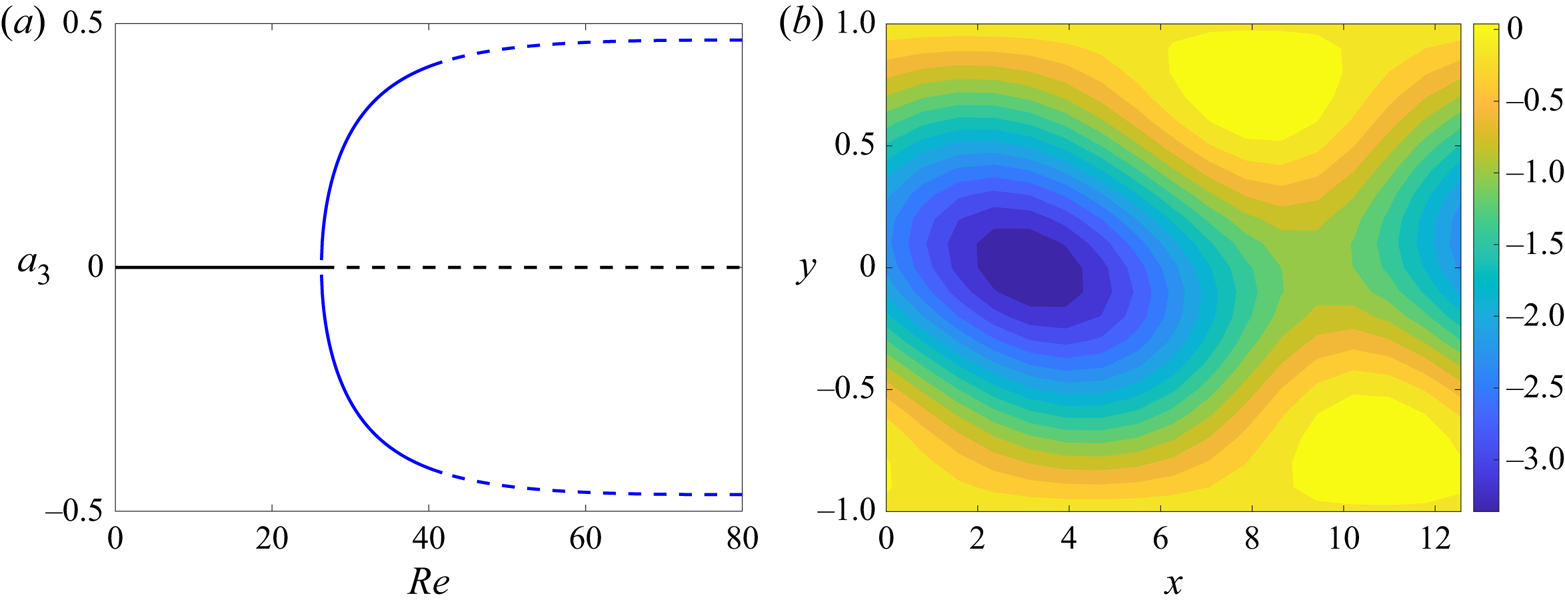
 $Re = 26.3$. For Reynolds numbers larger than this value there is one real positive eigenvalue, indicating the occurrence of a pitchfork bifurcation. This was confirmed to be a supercritical bifurcation by a search for fixed points, whose results are shown in figure 2. The new fixed points are saturated two-dimensional vortex solutions, with non-zero amplitudes for the first four modes (the two-dimensional ones), and zero amplitudes for the remaining spanwise dependent modes. As the laminar solution and the body force are antisymmetric, these KH vortices have zero phase velocity and are thus a steady-state solution of the system after the pitchfork bifurcation. The two solutions differ only by an
 $L_x/2$ shift in the streamwise direction, which is expected due to the symmetry of the system. In what follows, we will consider these two solutions as ‘positive’ or ‘negative’ saturated vortex solutions based on the sign of
 $a_3$.
(a) First pitchfork bifurcation of the system. Full lines are stable fixed points, and dashed lines show unstable ones. The black line refers to the laminar solution, and the blue line shows the saturated vortex. (b) The  $z$-vorticity of the saturated vortex solution for
 $Re=35$.

These saturated vortex modes are in turn stable up to  $Re=41.8$. A pair of complex-conjugate eigenvalues become unstable for Reynolds number beyond this value. By integrating the nonlinear ROM in (2.12) we verified that this is a supercritical Hopf bifurcation: a low-amplitude limit cycle appears for
 $Re$ slightly larger than the critical value, and grows monotonically in amplitude for larger
 $Re$. The emerging limit cycle involves all modes, and thus leads to three-dimensional behaviour. This may be related to the instabilities of shear-layer vortices studied by Pierrehumbert & Widnall (Reference Pierrehumbert and Widnall1982), who have found that a periodic array of vortices has three-dimensional instabilities which may be either stationary (referred to as translational instability) or oscillatory (higher-order modes). The stationary mode is studied by Pierrehumbert & Widnall (Reference Pierrehumbert and Widnall1982) as leading to the emergence of steady streaks, and the oscillatory modes have a more complex structure. As the present limit cycle involves all modes, which oscillate at a non-zero frequency, we tentatively associate the observed instability with the higher-order modes by Pierrehumbert & Widnall (Reference Pierrehumbert and Widnall1982).
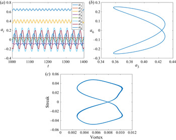
The behaviour of the system as a function of time for  $Re=50$, after the Hopf bifurcation, is illustrated in figure 3. The system has a similar behaviour of what was found in NC. Modes
 $a_1$ (mean-flow 1) and
 $a_6$ (streak) oscillate, with low values of
 $a_1$ occurring for large
 $|a_6|$, which can be thought of high-amplitude streaks and rolls (modes
 $a_5$ and
 $a_6$) leading to strong mean-flow distortions, reducing the mean shear. In turn, low (high) mean shear stabilises (destabilises) the vortex modes
 $a_3$ and
 $a_4$, which have an amplitude decay (growth). This has led the labelling of this cyclic behaviour as PAPU flow in NC, as the observation of the KH modes
 $a_3$ and
 $a_4$ alone gives the impression that the system oscillates between KH stable and KH unstable.
Limit-cycle oscillation for  $Re=50$ and comparison with DNS results from NC (
 $Re=200$ and no-slip boundary conditions). (a) Sample time series, (b) phase portrait of modes 3 and 6 and (c) DNS phase portrait of vortices and streaks, from NC.

A phase portrait involving  $a_3$ and
 $a_6$ is also shown in figure 3(b). The portrait has a distorted ‘8’ shape, with streaks,
 $a_6$ changing in sign and an amplitude variation of KH mode
 $a_3$ without sign change. For comparison, a phase portrait taken from the DNS in NC is shown in figure 3(c), with ‘streak’ and ‘vortex’ states obtained using the streamwise velocity at wavenumber
 $(k_x,k_z)=(0,\gamma )$ and
 $(\alpha,0)$, respectively, at
 $y=0.5$. As the DNS in NC uses no-slip boundary conditions, and is carried out at
 $Re=200$, only a qualitative comparison is possible, and thus the velocity fluctuations at this position and wavenumbers were deemed sufficient to evaluate a corresponding phase portrait from the DNS data. For both the present ROM and the NC data, large vortex amplitudes
 $a_3$ occur for low values of streak amplitude
 $|a_6|$, in the middle section of the ‘8’. Analysis of streaky shear layers (Marant & Cossu Reference Marant and Cossu2018) and jets (Lajús et al. Reference Lajús, Sinha, Cavalieri, Deschamps and Colonius2019; Wang et al. Reference Wang, Lesshafft, Cavalieri and Jordan2021), with steady streaks considered in a base flow, shows that they have a stabilising effect on the KH mechanism. The observed limit cycle, as for the one in NC, displays a similar behaviour, albeit in the nonlinear dynamics.
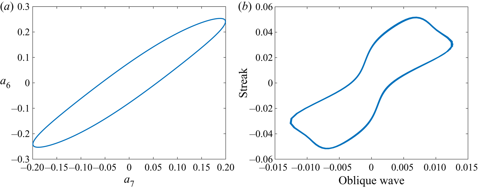
Oblique waves have an important role in defining the periodic behaviour of the model. As explored in NC, these waves grow exponentially with the vortices, and their phase is closely associated with the phase of streaks, such that alternation between positive and negative streaks is directly associated with the phase of these waves. This is exemplified in figure 4, displaying phase portraits from the model and from the DNS of NC. In the latter case, the ‘oblique wave’ state in the DNS was obtained by taking the streamwise velocity with  $(k_x,k_z) = (\alpha,\gamma )$ at
 $y=-0.5$. As in the results of figure 3, the comparison is only qualitative due to the different Reynolds number and boundary conditions, but the phase portraits show similar patterns, with a clear correlation between streaks and oblique waves.
Phase portraits of streaks and oblique waves in the limit-cycle oscillation for  $Re=50$ in the ROM, and
 $Re=200$ for the NC DNS data. (a) Phase portrait of modes 7 and 6 and (b) DNS phase portrait of streaks and oblique waves.

The significance of this limit cycle for the dynamics and sound radiation of jets is that it displays amplitude modulation of the KH mode  $a_3$ in time. This is known to be a mechanism of sound generation (Sandham, Morfey & Hu Reference Sandham, Morfey and Hu2006), especially when occurring simultaneously with amplitude modulation in space (Cavalieri et al. Reference Cavalieri, Jordan, Agarwal and Gervais2011). In a shear layer or jet, the latter is known to occur due to the spatial spreading of the shear layer, leading to the spatial decay of the KH mode in downstream regions (Jordan & Colonius Reference Jordan and Colonius2013; Cavalieri et al. Reference Cavalieri, Jordan and Lesshafft2019). Due to the homogeneity in
 $x$ of the present confined shear layer, represented by modes that are strictly periodic in
 $x$, an amplitude modulation in space is not possible. However, the observation of temporal modulation is relevant, and may be related to observations in turbulent jets, as discussed in NC. Notice that, due to the symmetry of the system, there is another stable limit cycle with
 $a_3<0$, which bifurcates from the lower branch of the vortex solutions in figure 2.
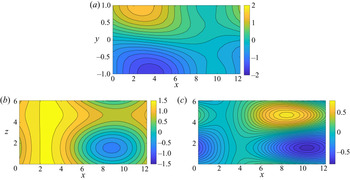
A visualisation of the velocity field for  $Re=50$, obtained with the ROM, is provided in figure 5. The instantaneous streamwise velocity
 $u$ is plotted in three chosen planes, for an instant corresponding to a maximal amplitude of the streak
 $a_6$. The chosen planes highlight vortices and streaks. In figure 5(a) an
 $x$–
 $y$ plane is shown, with a dominance of a vortex centred around
 $x=4$. Figures 5(b) and 5(c) display
 $x$–
 $z$ planes corresponding to the upper wall and shear-layer centre, respectively. The upper-wall visualisation of figure 5(b) shows that the vortex has a spanwise modulation, and the examination of figure 5(c) shows the presence of streaky structures. Such streaks are thus related to the spanwise variation of the velocity at the upper wall. The field thus shows a coexistence of vortices and streaks similar to the observations in NC. More precisely, the solution comprises not only vortices and streaks, but involves all eight modes, with varying amplitudes.
Visualisation of the streamwise velocity  $u$ at three chosen planes, for an instant that maximises streak amplitude
 $a_6$ with
 $Re=50$; (a)
 $x$–
 $y$ plane at
 $z=0$, (b)
 $x$–
 $z$ plane at
 $y=1$ and (c)
 $x$–
 $z$ plane at
 $y=0$.

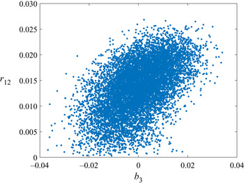
Nogueira & Edgington-Mitchell (Reference Nogueira and Edgington-Mitchell2021) have identified the presence of streamwise- elongated coherent structures in shock-containing twin jets by means of proper orthogonal decomposition applied to particle image velocimetry data. The two first dominant modes, whose temporal coefficients are denoted here as  $b_1$ and
 $b_2$, were associated with travelling waves in the resonance phenomenon, and are mainly dominated by a KH wavepacket. The third mode has a spatial support similar to the modes obtained by Nogueira et al. (Reference Nogueira, Cavalieri, Jordan and Jaunet2019); Pickering et al. (Reference Pickering, Rigas, Nogueira, Cavalieri, Schmidt and Colonius2020), and may thus be interpreted as a streak. Figure 6 shows the amplitude of the resonant cycle
 $r_{12}=(b_1^2+b_2^2)^{1/2}$ as a function of the streak amplitude
 $b_3$. It is clear that large positive/negative streak amplitudes are associated with large/small amplitudes of the resonant cycle. While these trends cannot be related quantitatively with the observations of the present ROM, they indicate that streaks modulate the amplitude of the vortices, which impacts the overall resonant phenomenon. Further analysis of turbulent-jet data may be able to uncover some of the nonlinear dynamics involving vortices and streaks.
Instantaneous values of KH wavepacket amplitude  $r_{12}$ as a function of streak amplitude
 $b_3$. Data from Nogueira & Edgington-Mitchell (Reference Nogueira and Edgington-Mitchell2021).

3.2. Transition to chaos for  $P=0.08$

As  $Re$ is increased beyond 41.8, the limit cycle of figure 3 develops with increasing amplitude. This cycle was tracked until
 $Re = 120$ by looking for time-periodic solutions of (2.12). The cycle stability was analysed using Floquet theory, as described by Kawahara et al. (Reference Kawahara, Uhlmann and Van Veen2012). The period of the limit cycle and its leading Floquet multipliers are shown in figure 7. There is always one multiplier equal to 1, corresponding to the neutral direction following the periodic orbit. With increasing
 $Re$ we observe a first instability appearing between
 $Re=52$ and 72.5. Inspection of the unstable Floquet multiplier shows that it is real and positive, and we thus have a crossing of the unit circle at
 $+1$. The cycle stability is restored at
 $Re=72.5$, and a secondary Hopf bifurcation, with complex conjugate Floquet multipliers leaving the unit circle, happens at
 $Re=109$. These instabilities are relevant for the appearance of chaotic behaviour, as will be shown in the next subsections.
Characteristics of the cycle emerging from the Hopf bifurcation at  $Re=41.8$. (a) Period of the cycle and (b) Absolute value of 3 leading Floquet multipliers.

3.2.1. Symmetry breaking
The numerical solutions of the system in this range of  $Re$ show that we have a symmetry-breaking bifurcation at
 $Re=52$, followed by symmetry restoring at
 $Re=72.5$. To show this behaviour, a Poincaré section is defined at the hyperplane
 $a_5=0$, and we collect points for the nonlinear simulation crossing the plane with
 $\dot {a}_5<0$. Thus, the behaviour of the dynamical system may be tracked with the Poincaré section that defines a map. This is carried out successively for Reynolds number varying in small increments, with the final state of the previous simulation taken as initial condition for the following one to minimise transients. Simulations with duration
 $T=2000$ are carried out and the points in the Poincaré section are kept only for the final half of the simulation. With this procedure we analyse systematically the attractor for each
 $Re$, without significant transient effects. The resulting points in the Poincaré section can be plotted as a function of Reynolds number, illustrating the changes in the behaviour of the system: a stable limit cycle becomes a fixed point in the Poincaré section; in case of period doubling, a period-
 $n$ periodic orbit appears as
 $n$ points in the section; a quasi-periodic attractor is a dense region; and chaos is also manifest by the lack of periodicity. The same approach was used by Kashinath, Waugh & Juniper (Reference Kashinath, Waugh and Juniper2014) in the analysis of the nonlinear dynamics of a thermoacoustic system. As discussed previously, the present system has two limit cycles, one with
 $a_3>0$ and another with
 $a_3<0$. The following results show only the dynamics related to the
 $a_3>0$; however, mirror solutions with
 $a_3<0$ also exist due to the symmetry of the problem.
The Poincaré section for  $Re$ between 42 and 80 is shown in figure 8(a). For
 $Re<52$ the system has a single stable limit cycle, which becomes a point in the Poincaré section for each
 $Re$. As the Reynolds number is increased beyond 52, the cycle becomes unstable and two other periodic solutions emerge in a symmetry-breaking bifurcation. A sample phase portrait for
 $Re=54$, is shown in figure 8, where we see that the symmetry of the ‘8’ shape is broken. Such asymmetric solutions suffer a symmetry-restoring bifurcation at
 ${Re=72.8}$, and the limit cycle analysed in § 3.1 becomes stable again. Both bifurcations are supercritical, as they do not show hysteresis.
Illustration of the symmetry-breaking and -restoring bifurcations. Phase portraits in (b) correspond to the red and blue branches shown in (a). (a) Poincaré section and (b) phase portrait for  $Re=54$.

3.2.2. Formation of a chaotic saddle
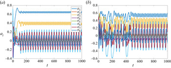
A difference between the dynamics before and after symmetry breaking and restoring is the appearance of transient chaos. This behaviour is illustrated in figure 9. Whereas the system quickly settles into the limit cycle for  $Re=50$, for
 $Re=80$ the modes display chaotic oscillations for a long transient before finally settling into the stable limit cycle. This suggests the existence of a chaotic saddle, similar to observations in ROMs of wall turbulence (Eckhardt & Mersmann Reference Eckhardt and Mersmann1999; Moehlis et al. Reference Moehlis, Faisst and Eckhardt2004). Such saddle attracts neighbouring states by its stable manifold, and the dynamics remains in the close vicinity of the saddle for a long transient until it is eventually repelled by the unstable manifold.
Transients leading to time-periodic behaviour. The system displays transient chaos for  $Re=80$; (a)
 $Re=50$ and (b)
 $Re=80$.

The origin of the chaotic saddle may be tracked by following a Poincaré section with fixed  $Re$ and varying
 $P$. This was carried out for
 $Re=54$, which for
 $P=0.08$ has two asymmetric limit cycles, as shown in § 3.2.1. The Poincaré section, calculated as in figure 8 is shown in figure 10(a). As
 $P$ is increased with fixed
 $Re$, the system undergoes a symmetry-breaking bifurcation for
 $P=0.077$. A further increase of
 $P$ leads to a saddle-node bifurcation for
 $P=0.0837$, seen in figure 10(a) as a jump in the value of
 $a_3$ in the Poincaré section. This bifurcation is not primarily relevant for the emergence of a chaotic saddle; further details are shown in Appendix A, where it is shown that the jump in
 $a_3$ is related to two saddle-node bifurcations. The limit cycles for
 $P>0.0837$ remain asymmetric as in figure 8. For
 $P=0.0857$ the cycles undergo a period-doubling bifurcation, starting Feigenbaum cascades leading to chaos for
 $P\approx 0.0874$. The cascade for one of the attractors is shown in more detail in figure 10(b).
Poincaré section for  $Re=54$ and varying
 $P$. Blue and red dots show sections tracked with one of the two asymmetric limit cycles of figure 8. (a) Full view and (b) detail of period-doubling cascade.

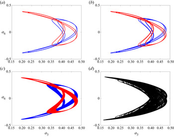
Up to  $P=0.088$ the two attractors remain distinct, with chaos confined to a low range of values of
 $a_3$. For
 $P$ beyond this value, the chaotic attractors undergo a merging crisis, as they simultaneously collide with their basin boundaries. This is seen in figure 10(a) as it becomes no longer possible to distinguish between blue and red dots. The merging crisis leads to an attractor that is larger than the previous ones combined, as observed by Chian et al. (Reference Chian, Borotto, Rempel and Rogers2005). Sample phase portraits are shown in figure 11, highlighting the sequence of events: the limit cycles undergo period doubling, as illustrated in figure 11(a,b), and become chaotic in panel (c). Such chaotic attractors remain distinct, and the system does not go from one to the other. A further increase of
 $P$ leads to the merging crisis, with a larger merged attractor in figure 11(d).
Phase portraits of attractors for  $Re=54$ and selected
 $P$. Blue and red lines show attractors with the convention of figure 10. The larger attractor for
 $P=0.09$ results from the merging crisis of the individual chaotic attractors shown in (c); (a)
 $P=0.0865$, period-2 cycle, (b)
 $P=0.0872$, period-4 cycle, (c)
 $P=0.088$, chaotic attractors and (d)
 $P=0.09$, merged chaotic attractor.

We conjecture that the boundary between the basins of attraction of the blue and red pre-crisis attractors is fractal. It is a known fact in dynamical systems that fractal basin boundaries can be formed by the stable manifold of a chaotic saddle (Battelino et al. Reference Battelino, Grebogi, Ott, Yorke and Yorke1988; Rempel et al. Reference Rempel, Chian, Koga, Miranda and Santana2008). At the merging crisis, both attractors simultaneously collide with the chaotic saddle and its stable manifold at the basin boundary and the three sets (two attractors and a chaotic saddle) merge to form the post-crisis chaotic attractor. The presence of the chaotic saddle is the reason why the post-crisis attractor is larger than the union of the two pre-crisis attractors.
The period-doubling cascade and subsequent merging crisis explain the emergence of a chaotic attractor at larger  $P$, for instance
 $P=0.09$ as shown in figures 10 and 11(d). A chaotic attractor comprises an infinite number of unstable periodic orbits, and the dynamics is related to stable and unstable manifolds of such orbits (Cvitanović & Eckhardt Reference Cvitanović and Eckhardt1989). For
 $P=0.08$ the dynamics eventually converges to the stable limit cycle; however, during transients, which become quite long for higher
 $Re$, the behaviour is nonetheless chaotic, as illustrated in figure 9(b). This may now be explained by the infinity of unstable periodic orbits that arise with the chaotic attractor for larger
 $P$. For
 $P=0.08$ such orbits are no longer able to retain indefinitely state-space trajectories, forming thus a chaotic saddle. However, during transients the system remains with a dynamics similar to that observed for the chaotic attractor for
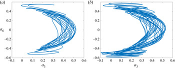
 $P=0.09$. This is illustrated in figure 12(a), which shows a phase portrait of a long transient taken for
 $P=0.08$ and
 $Re=80$. The system has a trajectory that closely resembles the chaotic attractor for
 $P=0.09$, shown in figure 12(b). Hence, the high-
 $P$ chaotic attractor loses stability and becomes a saddle for
 $P=0.08$, leading to the observed transients. Further analysis of the chaotic saddle for
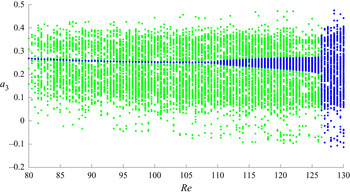
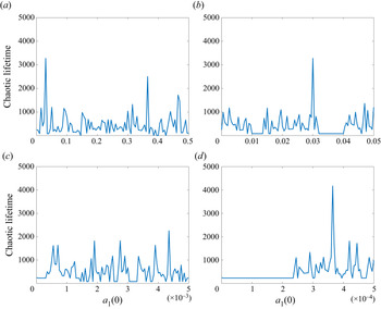
 $P=0.08$ is presented in Appendix B, showing its presence for
 $Re$ between 80 and 126.5 and the occurrence of long transient chaotic dynamics.
Phase portraits for  $Re=80$: (a) chaotic saddle with
 $P=0.08$ and (b) chaotic attractor with
 $P=0.09$.

3.2.3. Quasi-periodic and chaotic attractors
We now return to the stable limit cycle for  $P=0.08$, which is stable for
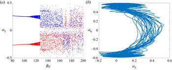
 $Re>72.5$ as seen in § 3.2.1. The Floquet analysis shown in figure 7 has a second crossing of the unit circle at
 $Re=109$, indicating instability. This time, complex conjugate Floquet multipliers leave the unit circle, in a secondary Hopf (or Neimark) bifurcation. This leads to a quasi-periodic attractor, whose behaviour may be seen in the plot of the Poincaré section shown in figure 13. Notice again that, due to the symmetry of the problem, two attractors are present, with either positive or negative values of
 $a_3$ (only the positive one is shown in figure 8); each one is tracked separately with increasing
 $Re$.
Emergence of a quasi-periodic attractor and its collision with the chaotic saddle. Panel (a) shows the Poincaré section for  $P=0.08$. Blue (red) dots show respectively sections tracked in
 $Re$, starting with the attractor with
 $a_3>0$ (
 $a_3<0$). Panel (b) shows a phase portrait of the attractor for
 $Re=130$.

Figure 13 shows that at  $Re=109$ the system transitions from a stable period-1 limit cycle to a quasi-periodic attractor, as indicated by the dense region that forms for
 $109< Re<126.5$. The appearance of the quasi-periodic attractor is illustrated in figure 14. For
 $Re=100$ the attractor is periodic, and the power spectral density (PSD) of figure 14(a) has peaks for a fundamental frequency
 $f_1\approx 0.05$ and its harmonics. Notice that, since the vortex mode
 $a_3$ was used to calculate the PSD, the dominant frequency corresponds to
 $2/T$, where
 $T~\approx 40$ is the period of the cycle shown in figure 7(a), since the oscillations in
 $a_3$ have a period that is half of the one for the streak mode
 $a_6$, for instance. Once the attractor becomes quasi-periodic, a second frequency
 $f_2\approx 0.03$, incommensurate with the previous one, appears in the PSD, as shown in figure 14(b). The time series now has oscillations with these two frequencies, and other ones that correspond to
 $af_1 + bf_2$ with integer
 $a, b$. In state space, the trajectories become a torus.
PSD of  $a_3$ for the attractor, discarding initial transients. Whereas the limit cycle for
 $Re=100$ is dominated by
 $f_1\approx 0.05$ and its harmonics, the quasi-periodic attractor for
 $Re=120$ has the appearance of a new frequency
 $f_2 \approx 0.03$, and the time series has peaks for frequencies given by integer multiples of
 $f_1$ added to integer multiples of
 $f_2$; (a)
 $Re=100$ and (b)
 $Re=120$.

By tracking the Poincaré section in figure 13 we notice a transition of the quasi-periodic behaviour to larger chaotic attractors at  $Re=126.5$. Such chaotic attractors are the continuation of the chaotic saddle studied in § 3.2.2: the sample phase portrait in figure 13(b) is close to the chaotic transient in figure 12(a) and the higher-
 $P$ attractor in figure 12(b). From the observation of the Poincaré section, we may conclude that the quasi-periodic attractor collides with the chaotic saddle at
 $Re=126.5$. It is not straightforward to demonstrate such a collision in a system with more than 3 degrees of freedom, since the Poincaré section still has high dimension and allows an apparent crossing of trajectories, which cannot occur in state space. However, due to the resemblance between chaotic attractor at larger
 $Re$ and the saddle at lower
 $Re$ it is likely that such collision occurs, leading to the disappearance of the quasi-periodic attractor and the emergence of persistent chaos.
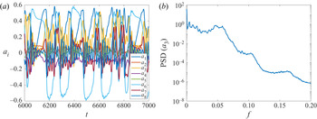
We confirm the properties of a chaotic attractor by further inspection of the solutions of the system for  $Re>126.5$. A sample time series for the eight modes is shown in figure 15(a), where no periodicity is evident. The PSD for the KH mode
 $a_3$ is shown in figure 15(b), showing a broad band behaviour, unlike the spectra of periodic and quasi-periodic attractors in figure 14. The chaotic behaviour is confirmed by a computation of the leading Lyapunov exponent
 $\lambda _1$ of the system, following Parker & Chua (Reference Parker and Chua2012). This leads to
 $\lambda _1=0.0186$, a positive value indicating exponential divergence of neighbouring solutions in the attractor, confirming that the system has a marked sensitivity to initial conditions, and is thus chaotic.
Results for  $Re=130$. (a) Time series and (b) PSD of
 $a_3$.

Despite the more complex behaviour, the solution has features that are reminiscent of the periodic cycle observed for lower Reynolds numbers. The power spectrum of figure 15(b) shows a broadband peak around  $f=0.05$, which is also the peak frequency of the limit cycle shown in figure 14(a). Moreover, inspection of the time series in figure 15(a) shows significant mean-flow distortions (low
 $a_1$) when streaks (
 $a_6$) have large amplitude. During these periods vortex modes, in particular
 $a_3$, remain with low amplitude. The eventual decay of streak amplitude leads to a recovery of the mean shear, and
 $a_1$ rises to values around 0.5. Once this happens, vortices grow again via the KH mechanism, until they are quenched by the mean-flow distortion due to a new high-amplitude streak. The amplitude modulation described in § 3.1 is now a broad-band, intermittent phenomenon. This can be tentatively compared with observations from turbulent jets, with intermittent events (Hileman et al. Reference Hileman, Thurow, Caraballo and Samimy2005; Akamine et al. Reference Akamine, Okamoto, Teramoto and Tsutsumi2019) modelled as amplitude modulations of KH wavepackets (Cavalieri et al. Reference Cavalieri, Jordan, Agarwal and Gervais2011), or, alternatively, as intermittent, transient growth of wavepackets (Schmidt & Schmid Reference Schmidt and Schmid2019). Clearly, care should be taken in drawing such connections between the present simplified ROM and realistic dynamics of high-
 $Re$ jets, but further exploration of jet data with the present mechanisms in mind appears to be promising.
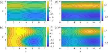
Visualisations of the instantaneous streamwise velocity for  $Re=130$ at
 $x$–
 $z$ planes are shown in figure 16. The same
 $x$–
 $z$ planes of figures 5(b) and 5(c) are taken, corresponding to the upper wall and shear-layer centre. The solution is shown at two times. The first one, shown in figures 16(a) and 16(b), corresponds to a time when the solution is dominated by the streak mode
 $a_6$, as observed in the time series of figure 15(a). The solution is dominated by the mean-flow and streak modes
 $a_1$ and
 $a_6$, with the vortex modes
 $a_3$ and
 $a_4$ with low amplitudes. The instantaneous streamwise velocity in figures 16(a) and 16(b) thus shows streaks at both upper wall and shear-layer centre. At other times, with comparable magnitudes of vortex and streak modes
 $a_3$ and
 $a_6$, the solution still displays streaks at the central plane (figure 16d), but the upper wall (figure 16c) shows the coexistence of vortices and streaks, perceived as a spanwise modulation of a vortical structure, similarly to the observation of the periodic cycle shown in figure 5.
Visualisation of the streamwise velocity  $u$ for
 $Re=130$ at two chosen planes, for a time with streak dominance (a,b) and a time with streak–vortex coexistence (c,d). (a) The
 $x$–
 $z$ plane at
 $y=1$,
 $t$ with streak dominance, (b)
 $x$–
 $z$ plane at
 $y=0$,
 $t$ with streak dominance, (c)
 $x$–
 $z$ plane at
 $y=1$,
 $t$ with vortex–streak coexistence and (d)
 $x$–
 $z$ plane at
 $y=0$,
 $t$ with vortex–streak coexistence.

3.3. Merging crisis
The Poincaré plot in figure 13 shows separate attractors up to  $Re=164.5$, represented with blue and red dots. Thus, for the periodic, quasi-periodic and chaotic attractors of the system the dynamics remains confined to either positive or negative
 $a_3$. The time series in figure 15(a), for instance, shows the evolution of the system for the attractor with mostly
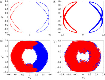
 $a_3>0$. Sample phase portraits of the various regimes are shown in figure 17, which displays both positive and negative periodic (a), quasi-periodic (b) and chaotic (c) attractors. For such Reynolds numbers, the system stays indefinitely at one of the attractors, and no numerical integration performed here showed any sign of switch. However, at
 $Re=164.5$ the chaotic attractors undergo a merging crisis, similar to what was seen in § 3.2.2. The present crisis leads to a larger attractor spanning both positive and negative
 $a_3$. The system spends extended periods with
 $a_3$ mostly of positive sign, and abruptly switches to mostly negative
 $a_3$. This is exemplified in the time series shown in figure 18, obtained for
 $Re=180$.
Phase portraits of attractors of the  $P=0.08$ system at selected Reynolds numbers. Blue and red lines show attractors with positive and negative
 $a_3$, respectively. Notice that, for
 $Re=180$, the attractors of lower
 $Re$ are already merged, thus blue and red lines refer to the same set. For the chaotic attractors,
 $\lambda _1$ is the largest Lyapunov exponent; (a)
 $Re=100$, periodic solution, (b)
 $Re=120$, quasi-periodic solution, (c)
 $Re=150$, chaotic attractor (
 $\lambda _1=0.0186$) and (d)
 $Re=180$, merged chaotic attractor (
 $\lambda _1=0.0202$).

Time series of mode 3 for  $Re=180$.

The interpretation of the results of figure 18 is that the time series of the merged chaotic attractor comprises extended periods where the system stays in a trajectory resembling one of the lower- $Re$ asymmetric chaotic attractors, as discussed by Grebogi et al. (Reference Grebogi, Ott, Romeiras and Yorke1987). In this case, close to the critical Reynolds number
 $Re_{cr}$ of the crisis, the typical lifetime of the solution at one of the original attractors, before switching to the other one, has an expected power-law behaviour
 $(Re-Re_{cr})^{\gamma }$, with
 $\gamma$ being a negative exponent. The lifetime statistics were obtained close to
 $Re_{cr}=164.8$, using the time series of vortex mode 3, low-pass filtered using a simple moving average, to detect if the solution is at its ‘mostly positive’ or ‘mostly negative’
 $a_3$ dynamics; given the observed time series, similar to the sample one shown in figure 18, detection of solution jumps with the proposed filter is straightforward. Statistics of the lifetimes at each state were thus obtained with long simulations, and are shown in figure 19. The lifetime closely follows a
 $(Re-Re_{cr})^{-2}$ dependence and supports the conclusion that a merging crisis occurs for this Reynolds number.
Lifetime of trajectories in an asymmetric chaotic saddle after the merging crisis at  $Re_{cr}=164.5$. The red line indicates a
 $(Re-Re_{cr})^{-2}$ dependence.

Past the merging crisis, the evolution of the KH mode  $a_3$ now involves modulation in amplitude and changes in phase. In the present model all modes are fixed at a given streamwise and spanwise position. As a single Fourier mode was included for each considered wavenumber, it is impossible to represent travelling waves or relative periodic orbits (which are periodic except for a spatial shift, e.g. Viswanath Reference Viswanath2007), and the only phases in
 $a_3$ are 0 or
 ${\rm \pi}$; alternatively, one may think of vortex positions at
 $x=0$ or
 $x=L_x/2$, and each jump in the merged chaotic attractor represents a phase jump in
 $a_3$. A more complete model would include two modes for each wavenumber, allowing a continuous change of phase. In this case, the dynamics of the larger, merged attractor would lead to continuous phase drifts of the vortices. This would represent a varying phase speed in addition to amplitude modulation.
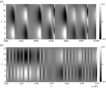
This feature can also be seen by increasing the Reynolds number of the DNS. Streamwise velocity fields at  $y=1.5141$ were extracted from a simulation at
 $Re=205$ (keeping the same numerics as in NC), and these are shown in figure 20(a). The streamwise averaged field was subtracted from the velocity to highlight the presence of the KH vortices. Figure 20 shows that, differently from the
 $Re=200$ case reported in NC, the dynamics of the flow for this Reynolds number is no longer periodic. In this case, vortices suffer a change in phase in some times, similar to the present model, with space–time behaviour of vortices reconstructed using
 $a_3$ and
 $\boldsymbol {u}_3$, taken at
 $y=1$. As in previous comparisons between ROM and DNS, quantitative agreement is not expected due to the no-slip conditions in the DNS, but the results show that both the DNS and ROM display phase jumps of
 ${\rm \pi}$ at specific times.
Vortices in the NC DNS for  $Re=205$, and in the present model for
 $Re=200$, illustrated by fluctuations of the streamwise velocity on
 $y=1$ for the ROM and for
 $y=0.5$ for the DNS. (a) DNS results, with the same configuration of NC, but at
 $Re=205$ and (b) ROM at
 $Re=200$.

It should be noted that the specific behaviour observed in the ROM is related to the low-order representation of KH vortices with a fixed phase in  $x$. The inclusion of additional modes to represent other possible phases in
 $x$ would allow more complex behaviours, with travelling waves (Wedin & Kerswell Reference Wedin and Kerswell2004) and relative periodic orbits (Viswanath Reference Viswanath2007) associated with continuous phase changes in the streamwise direction. Further work in this direction would be important to understand the chaotic behaviour observed in the vortex phase in an attempt to connect such observations with more realistic flows.
In summary, by studying the ROM with increasing Reynolds number we obtain a progressively richer dynamics, including limit cycles, quasi-periodic attractors, chaotic saddles and attractors. The low dimension of the model, involving eight modes, limits the dynamics to a minimal representation. Despite the low order of the system, the dynamics resembles observations of turbulent jets. The nonlinear interactions included in the present low-order system, shown in (2.12), point thus to phenomena of potential relevance in flows of interest. Further investigation of the nonlinear interactions in turbulent jets, using appropriate signal processing (Schmidt Reference Schmidt2020), is a promising direction, and the present ROM, as well as its solutions, may aid in the interpretation of data. The reduced number of nonlinear interactions in the model may also help in the development of nonlinear models for spatially developing shear layer and jets (Suponitsky et al. Reference Suponitsky, Sandham and Morfey2010; Wu & Zhuang Reference Wu and Zhuang2016; Zhang & Wu Reference Zhang and Wu2020).
4. Conclusions
The nonlinear dynamics of a shear layer is studied using a ROM. A shear layer confined between parallel walls and driven by a body force, introduced by NC, prevents the spatial development of the flow and thus allows the use of periodic boundary conditions in streamwise and spanwise directions, which greatly simplifies the problem. The same configuration is considered here, but instead of the no-slip boundary conditions used in the DNS in NC, we adopt free-slip boundary conditions on the parallel walls. This ensures that the confined shear layer does not develop near-wall fluctuations that would clearly be absent in free shear layers and jets. Moreover, by using free-slip boundary conditions, a ROM may be obtained using Fourier modes in all three spatial directions, and application of a Galerkin projection of the Navier–Stokes equation leads to a system of ordinary differential equations, similar to related works on wall-bounded turbulence (Waleffe Reference Waleffe1997; Moehlis et al. Reference Moehlis, Faisst and Eckhardt2004; Cavalieri Reference Cavalieri2021).
The procedure aims to build and study a simplified system in order to reveal the nonlinear dynamics of shear layers, which may shed light on the behaviour of spatially developing flows such as jets. Turbulent jets have been thoroughly studied using linearised models and input/output analysis in recent years (Garnaud et al. Reference Garnaud, Lesshafft, Schmid and Huerre2013; Jeun et al. Reference Jeun, Nichols and Jovanović2016; Schmidt et al. Reference Schmidt, Towne, Rigas, Colonius and Brès2018; Lesshafft et al. Reference Lesshafft, Semeraro, Jaunet, Cavalieri and Jordan2019), but features such as amplitude and phase modulation of KH wavepackets, referred to as ‘jitter’, are more challenging to model using linear theory. Jitter in amplitude and phase has been observed in numerical and experimental data and related to the sound radiation, with particular relevance for subsonic flows (Cavalieri et al. Reference Cavalieri, Jordan, Agarwal and Gervais2011; Baqui et al. Reference Baqui, Agarwal, Cavalieri and Sinayoko2015; Cavalieri et al. Reference Cavalieri, Jordan and Lesshafft2019). The analysis in NC used a direct numerical simulation of a confined shear layer, showing that the nonlinear dynamics leads to the appearance of a stable limit cycle with amplitude modulation of KH vortices, in a behaviour reminiscent of amplitude jitter seen in jet data. This direction is further pursued here by the construction of a ROM with the dominant structures studied in NC, which allows a more straightforward analysis of the nonlinear dynamics of the confined shear-layer configuration.
Eight modes were selected to build the ROM, based on the observations in NC. Such modes represent the mean flow, KH vortices, rolls, streaks and oblique waves. For the mean flow, vortices and oblique waves, a pair of Fourier modes were needed for each structure in order to ensure a consistent representation of the dynamics. The body force that drives the shear layer was taken as a sum of two Fourier modes, with the second parametrised by a forcing parameter  $P$ that is related to the growth rate of the KH instability of the laminar solution. The nonlinear dynamics of the resulting ROM could be analysed in some detail, thanks to the reduced computational cost to obtain numerical solutions and their stability analysis. This provides a picture of how the confined shear layer transitions to the limit cycle studied in NC, and how such cycle eventually transitions to chaotic behaviour as the Reynolds number is increased.
The first bifurcations identified for the ROM are a pitchfork leading to saturated vortex solutions, and a Hopf bifurcation leading to a stable limit cycle. This limit cycle resembles the observations in NC, with amplitude modulation of vortices related to oscillations in rolls, streaks and oblique waves. As the Reynolds number is increased, we observe the emergence of a chaotic saddle. This was studied by varying the forcing parameter  $P$, showing the emergence of chaotic attractors via a period-doubling cascade as
 $P$ is increased. Such attractors eventually merge and form a larger chaotic attractor for
 $P=0.09$. At
 $Re=80$ and
 $P=0.08$ such attractor loses stability and becomes a chaotic saddle, with transient chaos. Thus, most initial disturbances for
 $P=0.08$ and Reynolds number between 72.5 and 109 display transient chaotic behaviour which eventually settles into the stable limit cycle that emerged from the first Hopf bifurcation. Since the ROM has symmetries, with corresponding solutions obtained by considering shifts in the streamwise or spanwise direction, all such solutions appear in pairs, with one of them corresponding to a vortex mode
 $a_3>0$, and the other related to
 $a_3<0$. Such solutions display time-periodic (for the limit cycle) or aperiodic (for the chaotic saddle) modulation of vortex amplitude, a behaviour that resembles the jitter in amplitude observed in high Reynolds number jets.
A further increase of  $Re$ leads to the appearance of a quasi-periodic attractor at
 $Re=109$. This attractor collides with the chaotic saddle at
 $Re=126.5$, leading to the appearance of a chaotic attractor. The time series of the various modes show broadband behaviour, with no periodicity, in a more complex behaviour that approaches what is seen in turbulence. The symmetries of the system again imply that two chaotic attractors are formed, with positive or negative vortex time coefficient
 $a_3$. Such attractors suffer a merging crisis at
 $Re=164.8$, and become a larger chaotic attractor where solutions spend some time at one of the original attractors and then ‘jump’ to the other one. This implies that the solution starts to display jumps between positive and negative values of the vortex
 $a_3$, which in turn means that vortices have a
 ${\rm \pi}$ phase jump in
 $x$. Although in a much simplified manner, such phase jitter is again reminiscent of observations of KH wavepackets in turbulent jets. Thus, the present ROM may be thought as a minimal model that mimics to some extent jitter in amplitude and phase of KH vortices. Its modes and their interaction are minimal ingredients to obtain a dynamics that resembles observations of high-
 $Re$ jets.
Keeping in mind that several simplifications were applied to both the flow configuration (by considering a confined shear layer) and the underlying equations (by reducing the model using a Galerkin projection with eight modes), the present ROM opens a number of interesting directions for the study of turbulent free-shear flows. The ROM has closed-form equations that include nonlinear interactions between modes that have turbulent-jet counterparts, such as KH vortices (Cavalieri et al. Reference Cavalieri, Rodríguez, Jordan, Colonius and Gervais2013), rolls and streaks (Nogueira et al. Reference Nogueira, Cavalieri, Jordan and Jaunet2019). By studying the nonlinear interactions among the various structures in the model, one may better understand how the corresponding modes interact in turbulent jets, which is not possible using standard linear input/output analysis. The ROM displays clear correlations between vortices and streaks, which may be further investigated using dedicated signal processing of numerical or experimental databases.
It is clear that high Reynolds number jets will display a dynamics that is not captured by the model. However, it is hoped that the rich nonlinear dynamics displayed by the ROM may shed light on behaviours of more complex flows. In the past, ROMs of wall-bounded turbulence by Waleffe (Reference Waleffe1997) and Moehlis et al. (Reference Moehlis, Faisst and Eckhardt2004) helped to understand the relationship of rolls, streaks and sinuous disturbances, and showed that, under some conditions, turbulence in such configurations has finite lifetimes, an observation later confirmed by the experiments of Hof et al. (Reference Hof, Westerweel, Schneider and Eckhardt2006). ROMs were important in defining the concept of edge states between laminar and turbulent solutions (Skufca, Yorke & Eckhardt Reference Skufca, Yorke and Eckhardt2006), a concept later extended to wall-bounded flows using full direct numerical simulations (Schneider, Eckhardt & Yorke Reference Schneider, Eckhardt and Yorke2007; Duguet et al. Reference Duguet, Monokrousos, Brandt and Henningson2013). It is hoped that the present ROM will also enable a number of approaches based on dynamical systems theory, which may help probing the nonlinear dynamics of turbulent shear layers and jets.
Acknowledgements
A numerical implementation of the present ROMs is available by request to the first author.
Funding
This work was supported by FAPESP Grant No. 2019/27655-3 and CNPq Grant Nos 313225/2020-6 and 306920/2020-4.
Declaration of interests
The authors report no conflict of interest.
Appendix A. Saddle-node bifurcations of asymmetric limit cycles
This appendix briefly studies the saddle-node bifurcations of the asymmetric limit cycles studied in § 3.2.1. Figure 21(a) shows periodic solutions with  $Re=54$, and
 $P$ between 0.083 and 0.084. There are two stable limit cycles, shown with full lines, that are connected to an unstable cycle by saddle-node bifurcations for
 $P=0.08373$ and
 $P=0.08358$. This pair of saddle-node bifurcations leads to hysteresis, as shown in figure 21(b): as
 $P$ is increased above 0.083, the system remains in the lower-branch cycle until the first saddle-node bifurcation, where it jumps to the upper-branch solution. As
 $P$ is decreased from 0.084, the system remains in the upper branch until it reaches the second saddle-node bifurcation, where the solution jumps to the lower branch. This explains the jump observed in figure 8.
Saddle-node bifurcations for  $Re=54$: (a) period of periodic solutions, with full lines showing stable cycles and the dashed line showing the unstable one, and (b) Poincaré section at
 $a_5=0$ and
 $\dot {a}_5<0$, with arrows highlighting the path in the plot as
 $P$ is increased and then decreased.

Appendix B. Analysis of the chaotic saddle
We present here some further results related to the chaotic saddle analysed in § 3.2.2. Unlike an attractor, chaotic saddles display transient chaos. Such saddles may be studied using a grid of initial conditions, in the ‘sprinkler’ method proposed by Hsu, Ott & Grebogi (Reference Hsu, Ott and Grebogi1988). Statistics of the chaotic transients may then be obtained in the time period after the solutions approach the saddle, and before they drift away from it. A positive Lyapunov exponent, obtained by averaging several transients so obtained, confirms the chaotic nature of the saddle. Another property of such saddles is that it is possible to obtain arbitrarily long chaotic transients, also by sampling a grid of initial conditions (Nusse & Yorke Reference Nusse and Yorke1989). Chaotic saddles may emerge in various manners, such as by the occurrence of a boundary crisis (Grebogi, Ott & Yorke Reference Grebogi, Ott and Yorke1983; Grebogi et al. Reference Grebogi, Ott, Romeiras and Yorke1987), where a chaotic attractor collides with a fixed point or periodic orbit. Chaotic saddles can also be observed in relation to interior crises and fractal basin boundaries (Robert et al. Reference Robert, Alligood, Ott and Yorke2000; Rempel et al. Reference Rempel, Chian, Macau and Rosa2004, Reference Rempel, Chian, Koga, Miranda and Santana2008).
To further analyse the chaotic saddle in the present system, we applied the sprinkler method with 10 initial conditions for each Reynolds number. Such initial conditions were obtained using a state in the chaotic attractor with predominance of  $a_3>0$ for
 $P=0.08$ and
 $Re=130$ (blue attractor in figure 13), with each mode disturbed by a random number between
 $-$0.05 and 0.05. A Poincaré section for the chaotic transients as a function of
 $Re$ is shown in figure 22 with green dots. The attractors with dominance of
 $a_3>0$, shown in figure 13, are also shown in figure 22 with blue dots. The results of the sprinkler method show the existence of a chaotic saddle, for
 $80< Re<126.5$. The correspondence between the Poincaré section of the chaotic saddle for
 $Re<126.5$ and of the chaotic attractor for
 $Re>126.5$ further indicates that the quasi-periodic attractor of
 $Re<126.5$ collides with the chaotic saddle in an interior crisis, leading to the chaotic attractor for
 $Re>126.5$. Similar results are also obtained for the red attractor of figure 13, and are not shown here for brevity.
Poincaré section as a function of  $Re$ obtained for the attractor (blue dots) and the chaotic saddle (green dots), the latter obtained using the sprinkler method (Hsu et al. Reference Hsu, Ott and Grebogi1988).

Another feature of the chaotic saddle explored in a similar manner is the distribution of lifetimes of chaotic transients. We have studied the lifetimes for  $Re=80$, with an initial condition taken as a state at the chaotic attractor of
 $Re=130$, but with varying initial
 $a_1$. We again used the attractor with dominant
 $a_3>0$. Since the periodic orbit at
 $Re=80$ has strictly
 $a_3>0$, an occurrence of
 $a_3<0$ can only happen for a chaotic transient (as illustrated later, in figure 24). Accordingly, we took the last instant of time when
 $a_3<0$ as a lower bound of chaotic lifetime. Such lifetimes are shown in figure 23, with each subfigure displaying a refined version of the previous one. For some initial conditions, the solution quickly converges towards the stable periodic orbit, and the computed lifetime is approximately 200 time units or less. However, some initial conditions display much longer lifetimes, of more than a thousand time units. The results show an apparently fractal distribution of lifetimes, similar to the observations of Eckhardt & Mersmann (Reference Eckhardt and Mersmann1999) and Moehlis et al. (Reference Moehlis, Faisst and Eckhardt2004) in ROMs of wall-bounded turbulence.
Lifetimes of chaotic transients for  $P=0.08$,
 $Re=80$, with initial conditions with varying
 $a_1(0)$. Each successive panel is a refined version of the previous one, with a range of initial conditions shortened by a factor of 10.

To further illustrate the nature of the chaotic transients, the largest lifetime obtained in figure 23(d) is shown in figure 24, where we observe a long chaotic transient until  $t\approx 4100$, after which the solution converges to the stable periodic solution. Further sampling of initial conditions may lead to arbitrarily long transients (Nusse & Yorke Reference Nusse and Yorke1989), which may be used to calculate Lyapunov exponents of the chaotic saddle; however, this was not pursued here.
Illustration of a long chaotic transient, taken using the initial condition of figure 23(d) with largest chaotic lifetime.