







1. Introduction
Several applications in the chemical process industry involve gas–liquid flow through packed beds, e.g. hydrodesulphurisation of petroleum fractions using trickle bed reactors, catalytic hydrogenations and gas clean-up using absorption columns. The overall performance of these processes is a strong function of local liquid distribution. The liquid spreading inside packed beds is substantially influenced by the gas–liquid interaction (defined by gas and liquid flow rates, viscosity, density, surface tension, etc.), fluid–solid interaction (i.e. wettability), and particle characteristics (such as particle shape and size) other than the operating conditions. The dynamics of liquid spreading is governed by inertial force exerted by the injected liquid stream; the viscous force which resists the motion of liquid; the capillary force which either drives or resists liquid spreading depending on the wettability of particles; and gravitational force which either acts in the direction of flow or opposite based on the operating mode of these processes.
Eulerian multiphase models are widely used to predict the macroscopic (bed-scale) liquid spreading in packed beds as a function of the aforementioned parameters. In this approach, the fluid phases are assumed to be in an interpenetrating continuum, and the contributions of the governing forces are accounted for using semi-empirical models, e.g. the capillary force is incorporated using one of the models proposed by Attou & Ferschneider (Reference Attou and Ferschneider1999), Grosser, Carbonell & Sundaresan (Reference Grosser, Carbonell and Sundaresan1988) or Lappalainen, Manninen & Alopaeus (Reference Lappalainen, Manninen and Alopaeus2009); the cumulative effect of inertial and viscous force is accounted for using the interphase momentum exchange (proposed by Attou & Ferschneider Reference Attou and Ferschneider1999) and mechanical dispersion (proposed by Lappalainen et al. Reference Lappalainen, Manninen and Alopaeus2009) models. In order to establish a reasonable agreement between the predictions of Eulerian multiphase model and measurements, the semi-empirical capillary force and/or the interphase momentum exchange models are either modified and/or the contribution of the mechanical dispersion force model is neglected (see Jindal & Buwa (Reference Jindal and Buwa2017), Dhanraj & Buwa (Reference Dhanraj and Buwa2018) and articles cited therein for further details). Therefore, to understand the physics of liquid spreading in packed beds and to improve the force models used in the Eulerian multiphase framework, it is essential to comprehend how different forces contribute to the dynamics of liquid spreading at the particle scale, and the corresponding void-scale flow behaviour.
Several researchers have investigated two-phase flow through porous media (characterised by length scales of a few micrometres) at the particle/pore scale using measurements and numerical simulations. Many of these studies investigate two-phase flows in horizontal configurations wherein, the effect of gravitational force is negligible. With the aid of measurements and simulations (e.g. Ambekar, Mondal & Buwa (Reference Ambekar, Mondal and Buwa2021), Holtzman & Segre (Reference Holtzman and Segre2015), Hu et al. (Reference Hu, Lan, Wei and Chen2019), Lenormand (Reference Lenormand1990), Lenormand, Touboul & Zarcone (Reference Lenormand, Touboul and Zarcone1988), Primkulov et al. (Reference Primkulov, Pahlavan, Fu, Zhao, MacMinn and Juanes2021, Reference Primkulov, Pahlavan, Fu, Zhao, MacMinn and Juanes2019), Wang et al. (Reference Wang, Pereira, Sauret and Gan2022), Xiao et al. (Reference Xiao, Zhu, Zhang, Yao and Sun2021) and Zhao, MacMinn & Juanes (Reference Zhao, MacMinn and Juanes2016)), it is shown that such a two-phase flow phenomenon is governed by the interplay between capillary and viscous force. Therefore, the two-phase flow phenomenon is investigated with the aid of capillary number (ratio of viscous to capillary force) and viscosity ratios. These investigations have subsequently resulted in the identification of various two-phase flow regimes, i.e. stable, viscous and capillary fingering as a function of capillary number and viscosity ratio. The aforementioned information is further used to propose regime maps for two-phase flow through porous media. A few studies also report the investigation of two-phase flow phenomena through porous media under the influence of gravitational force (e.g. Breen et al. (Reference Breen, Pride, Masson and Manga2022), Dong, Yan & Li (Reference Dong, Yan and Li2011), Islam et al. (Reference Islam, Chevalier, Salem, Bernabe, Juanes and Sassi2014) and Zheng et al. (Reference Zheng, Mahabadi, Yun and Jang2017)). These studies show that the viscous fingering is promoted by gravitational force if it acts in the direction of flow whereas, it stabilises viscous fingering if it acts in the direction opposite to the flow direction depending on the magnitude of Bond number (ratio of gravitational to capillary force). Although these studies provide insights into the two-phase flow regimes and their relationship with governing forces (i.e. dimensionless numbers), they do not provide information on how different forces influence the pore/particle-scale two-phase flow phenomena at different temporal stages.
With the increasing affordability of computational resources, interface-resolved methods (such as volume-of-fluid (VOF), level set (LS) and phase field (PF)) can be used to simulate liquid spreading in structure/particle-resolved domains. The predictions of these simulations do not rely on semi-empirical models and, thus, can be used to understand the role of various forces governing the dynamics of liquid spreading. Recently, such simulations have been used to understand the role of various forces on the spreading of a single droplet over a porous medium (Frank & Perre Reference Frank and Perre2012; Das et al. Reference Das, Patel, Milacic, Deen and Kuipers2018; Fu et al. Reference Fu, Li, Wang and Wu2019; Shi et al. Reference Shi, Tang, Lin, Zhao and Cheng2019; Ezzatneshan & Goharimehr Reference Ezzatneshan and Goharimehr2020). Subsequently, the time evolution of droplet spreading is subdivided into inertial, capillary and viscous regimes depending on the relative importance of different forces. However, the two flow systems, i.e. spreading of a droplet over a porous medium and spreading of a continuous liquid stream inside a packed bed, are substantially different. Concerning liquid spreading in packed beds, the interface-resolved (VOF) simulations are used to investigate the influence of fluid properties, operating conditions (e.g. Lopes & Quinta-Ferreira Reference Lopes and Quinta-Ferreira2009, Reference Lopes and Quinta-Ferreira2010), wettability (e.g. Du et al. Reference Du, Zhang, Lv, Lu, Xu and Wei2015, Reference Du, Zhang, Lu, Xu, Wei, He and Zhang2017) and particle shape (Kang et al. Reference Kang, Ciou, Lin, Wong and Jang2019; Deng et al. Reference Deng, Guo, Dong, Liu and Geng2020) on the steady-state liquid distribution. However, the effect of the aforementioned parameters on the contribution of different forces at different temporal stages of liquid spreading and their relationship with void-scale flow behaviour has not been explored. The understanding of the dynamics of various forces and its relationship with the time evolution of local liquid spreading is crucial for the improvement/development of force models for continuum approaches.
In the present study, a three-dimensional (3-D) bed randomly packed with 440 uniformly sized spherical particles is created by mimicking the process of particles falling inside a box under the influence of gravity using rigid body simulations. The VOF method implemented in the open-source flow solver OpenFOAM, is used to simulate the time evolution of liquid spreading inside the small section of the packed bed. Further, the role of governing forces at different temporal stages of liquid spreading influenced by capillary, inertial and gravitational force, is quantified using dimensionless numbers such as Ohnesorge, Weber and  $AB_i$ (proposed in the present work). Moreover, the relationship between dimensionless numbers and the void-scale interface dynamics is established.
2. Problem formulation
The dynamics of liquid spreading in the small section of the packed bed is investigated using the VOF model implemented in the finite-volume-based open-source code OpenFOAM v6. In order to create a particle-resolved fluid domain, initially, a large bed (10  $d_p\times 17$
 $d_p\times 15$
 $d_p$) of spherical particles is created by mimicking the process of filling a box randomly with uniformly sized particles (diameter
 $d_p = 4$ mm) under the influence of gravity using rigid body simulation, performed using the open-source software Blender v2.83. Due to the sharp intersection angles, the particle–particle contact regions were difficult to mesh and, therefore, the particles were shrunk radially by 2 %. The particles were then subtracted from the box volume to create the void-volume/fluid domain. The near-wall regions (equivalent to 3.5
 $d_p$ from the box wall) of the fluid domain were trimmed to exclude the wall-influenced large voids resulting in a bed with dimensions 3
 $d_p\times 10$
 $d_p\times 8$
 $d_p$ containing approximately 440 particles as shown in figure 1.
Computational domain with boundary conditions.

The fluid domain (shown in figure 1) is filled with air (viscosity  $\mu _a = 1.48 \times 10^{-5}$ Pa s and density
 $\rho _a = 1$ kg m
 $^{-3}$). Water (viscosity
 $\mu _w = 1 \times 10^{-3}$ Pa s and density
 $\rho _w = 1000$ kg m
 $^{-3}$) is injected at a constant flow rate
 $Q_w$ of
 $3.14 \times 10^{-6}$ m
 $^{3}$ s
 $^{-1}$ from the small circular inlet (
 ${\rm diameter} = d_p/2$) located centrally on the top cut-plane (
 $XY$ plane at
 $Z = 8$
 $d_p$) in the negative
 $Z$-direction (see figure 1). Gravity
 $g$ also acts in the flow direction (negative
 $Z$-direction). Three values of gas–liquid surface tension
 $\sigma _{aw}$, i.e. 70, 40 and 10 mN m
 $^{-1}$, are considered to study the effect of
 $\sigma _{aw}$ on the dynamics of liquid spreading. In the present study, the fluids are assumed to be Newtonian and incompressible.
2.1. Governing equations
In the VOF method (Hirt & Nichols Reference Hirt and Nichols1981), a single set of continuity (2.1) and momentum (2.2) equations is solved:
 $$\begin{gather} \boldsymbol{\nabla}\boldsymbol{\cdot}\boldsymbol{\bar{v}} = 0, \end{gather}$$
 $$\begin{gather}\frac{\partial}{\partial t}(\rho\boldsymbol{\bar{v}}) + \boldsymbol{\nabla}\boldsymbol{\cdot}(\rho\boldsymbol{\bar{v}}\boldsymbol{\bar{v}}) ={-}\boldsymbol{\nabla}{p} + \mu\nabla^2\boldsymbol{\bar{v}} + \boldsymbol{\bar{F}{_s}} + \rho\boldsymbol{\bar{g}} , \end{gather}$$
where  $\boldsymbol {\bar {v}}$ is the velocity (m s
 $^{-1}$),
 $p$ is the pressure (Pa) and
 $\boldsymbol {\bar {F}{_s}}$ is the surface tension force per unit volume (N m
 $^{-3}$). Here
 $\rho$ and
 $\mu$ are the phase volume fraction weighted density (kg m
 $^{-3}$) and viscosity (Pa s) and are computed as
 \begin{equation} \rho = \alpha_w\rho_w + (1-\alpha_w)\rho_a \quad {\rm and}\quad \mu = \alpha_w\mu_w + (1-\alpha_w)\mu_a, \end{equation}
where  $\alpha _w$ and
 $\alpha _a$ (
 $=1-\alpha _w$) are the volume fractions of water and air, respectively.
The motion of the air–water interface is simulated by solving the advection equation for  $\alpha _w$ (2.4),
 \begin{equation} \frac{\partial}{\partial t}(\alpha_w\rho_w) + \boldsymbol{\nabla}\boldsymbol{\cdot}(\alpha_w\rho_w\boldsymbol{\bar{v}}) + \boldsymbol{\nabla}\boldsymbol{\cdot}(\alpha_w (1-\alpha_w) \boldsymbol{\bar{u}{_r}})= 0, \end{equation}
where  $\boldsymbol {\bar {u}{_r}}$ is compression velocity and the third term on the left-hand side of (2.4) is an artificial compression term used to limit numerical diffusion (see Nekouei & Vanapalli (Reference Nekouei and Vanapalli2017) and articles cited therein for details). The Multidimensional Universal Limiter with Explicit Solution (MULES) algorithm is also used to correct the
 $\alpha _w$ fluxes to ensure boundedness and conservativeness (see Greenshields (Reference Greenshields2018) for details).
Here  $\boldsymbol {\bar {F}{_s}}$ is computed using the continuum surface force (CSF) model, proposed by Brackbill, Kothe & Zemach (Reference Brackbill, Kothe and Zemach1992), given as
 \begin{equation} \boldsymbol{\bar{F}{_s}} ={-}\sigma_{aw}\kappa\boldsymbol{\nabla}{\alpha_w}, \end{equation}
where  $\kappa$ is the local curvature of the gas–liquid interface and is calculated from the local gradients of the surface normal (
 $\boldsymbol {\hat {n}}$) of the interface as
 $\kappa = \boldsymbol {\nabla }\boldsymbol {\cdot }\boldsymbol {\hat {n}}$, where
 $\boldsymbol {\hat {n}} = \boldsymbol {\nabla }\alpha _w/|\boldsymbol {\nabla }\alpha _w|$.
2.2. Boundary conditions
A constant velocity along with  $\alpha _w = 1$ is specified at the liquid inlet. The remaining portion of the top cut-plane is specified with a constant pressure of 1 atm with
 $\alpha _w = 0$ (at time
 $t = 0$). A pressure outlet boundary condition (
 $p = 1$ atm) is specified at the bottom cut-plane (
 $XY$ plane at
 $Z = 0$, figure 1) along with backflow
 $\alpha _w$ of 0. The symmetry boundary condition is specified at the lateral cut-planes (
 $XZ$ planes at
 $Y = 0$ and 10
 $d_p$). A no-slip boundary condition is specified at the particle surfaces and the front and rear cut-planes (
 $YZ$ plane at
 $X = 0$ and 3
 $d_p$, respectively) as shown in figure 1. Here,
 $\kappa$ (in (2.5)) in cells adjacent to particle surfaces and front/rear cut-planes was defined by specifying
 $\boldsymbol {\hat {n}}$ as
 $\boldsymbol {\hat {n}} = \boldsymbol {\hat {n}{_w}}\cos {\theta {_w}} + \boldsymbol {\hat {t}{_w}}\sin {\theta {_w}}$, where
 $\theta _w$ is the static three-phase contact angle measured inside the liquid phase,
 $\boldsymbol {\hat {n}{_w}}$ and
 $\boldsymbol {\hat {t}{_w}}$ are the unit vectors normal and tangential to the faces with no-slip boundary, respectively, as shown in figure 2. In the present work, a
 $\theta _w$ of 90
 $^{\circ }$ is specified on front/rear cut-planes rendering them neutrally wet. Thus, the lateral spreading of the continuous liquid stream inside the particle-resolved fluid domain is simulated.
Interpretation of  $\theta _{w}$ in the CSF–VOF method.

2.3. Dimensionless numbers
As mentioned in § 1, the dynamics of liquid spreading is governed by inertial, viscous, capillary and gravitational forces. As discussed later, the inertial and capillary force promote liquid spreading in the lateral direction, whereas the gravitational forces limits the lateral liquid spreading by driving liquid in the vertical direction. Moreover, the viscous force resists the motion of liquid in all directions. As the objective of the present study is to understand the relative contribution of these forces in the dynamics of lateral liquid spreading, the following dimensionless numbers are considered:
 $$\begin{gather} \mbox{Ohnesorge},\ Oh = \mu_w/\sqrt{\rho_w{d_V}\sigma_{aw}\cos\theta_{w}} \equiv \mbox{Viscous}/(\sqrt{\mbox{Inertial}\times\mbox{Capillary}}), \end{gather}$$
 $$\begin{gather}\mbox{Newly proposed},\ AB_i = \frac{{V_i}}{g}\sqrt{\frac{\sigma_{aw}\cos\theta_{w}}{\rho_w{d_V}^3}} \equiv \sqrt{\frac{\mbox{Inertial}\times\mbox{Capillary}}{\mbox{Gravity}}}, \end{gather}$$
where  $d_V$ is the average void size (
 $d_p$/2.61 for the present domain) determined using the watershed algorithm (proposed by Rabbani, Jamshidi & Salehi Reference Rabbani, Jamshidi and Salehi2014) and
 $V_i$ is the velocity scale, which provide the ratio of forces driving lateral spreading to forces resisting the motion of liquid in the lateral direction. Further, to identify the relative dominance of the forces driving lateral liquid spreading the Weber number (
 $We_i$) defined as
 \begin{equation} We_i = \rho_w{d_V}{V_i}^2/\sigma_{aw}\cos\theta_{w} \equiv \mbox{Inertial/Capillary} \end{equation}
was used.
In the definition of aforementioned dimensionless numbers,  $d_V$ is considered as the characteristic length scale, as we intend to comprehend the motion of the gas–liquid interface through the void-resolved bed. The
 $AB_i$ and
 $We_i$ numbers are defined using two velocity scales: superficial liquid velocity (
 $V_s$) and area-average velocity of the gas–liquid interface (
 $V_I$), where the gas–liquid interface is defined by the iso-surface of
 $\alpha _{w} = 0.5$ (see figure 3). The values of
 $AB_s$ and
 $We_s$, which are based on
 $V_s$, can be predefined and are specific to a certain case. The absolute domain size was scaled by a factor of 0.5 and 2 in all directions such that it represents fluid domain with
 $d_p$ of 2 and 8 mm, respectively, without influencing the void topology. The values of
 $\sigma _{aw}$ as well as
 $\theta _{w}$ were varied such that they represent a range of
 $AB_s$ and
 $We_s$ values. The case-specific values of
 $AB_s$ and
 $We_s$ are listed in table 1. Thus, we investigate the dynamics of liquid spreading influenced by capillary or inertial (
 $AB_s\sim 1$), and gravitational force (moderately (
 $AB_s\sim 10^{-1}$) and strongly (
 $AB_s\sim 10^{-2}$)).
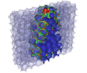
Liquid distribution (represented by iso-volume of  $\alpha _{w} \geq 0.5$ and indicated by blue colour) at
 $AB_s$ of (a) 2.37, (b)
 $2.01 \times 10^{-1}$ and (c)
 $1.85 \times 10^{-2}$ at breakthrough ‘
 $t^*$’ (note: the two-phase interface (defined by iso-surface of
 $\alpha _{w} = 0.5$) is coloured with the velocity magnitude. Further, the values of
 $We_s$ and
 $Oh$ corresponding to the values of
 $AB_s$ are stated in table 1).

Values of dimensionless numbers defined using  $V_s$ as the velocity scale.

Table 1 also states that the values of  $Oh$ are smaller than
 $10^{-2}$, indicating that the relative magnitude of viscous force is substantially smaller than the inertial and capillary forces for cases presented in the current work. Moreover, the values of
 $AB_s$ show that the magnitude of gravitational force is either comparable to or larger than the inertial and/or capillary forces. Therefore, we find that the contribution of viscous force is negligible as compared with other forces in the cases considered in the present work. Further, the definition of
 $AB_I$ and
 $We_I$, which considers
 $V_I$ as the characteristic velocity scale, vary with time as
 $V_I$ vary temporally and their time evolution is used to understand the interplay of governing forces at different stages of liquid spreading. Further, as the capillary force scales as a cosine function of
 $\theta _{w}$, as established by the Young–Laplace equation, the
 $\sigma _{aw}$ is scaled with
 $\cos \theta _{w}$ to consider the effect of wettability in the definition of all the above-mentioned numbers (2.6)–(2.8).
3. Results and discussion
Before performing the simulations of liquid spreading in the 3-D bed of spherical particles, the predictions of 3-D VOF simulations of liquid spreading in pseudo-two-dimensional (2-D) bed (consisting of cylindrical pillars of diameter 3 mm and length 1.5 mm arranged in a square pitch of 4.5 mm) were compared with the measurements by Horgue et al. (Reference Horgue, Augier, Duru, Prat and Quintard2013). As the VOF method reasonably predicted liquid spreading in a pseudo-2-D bed, it is used to investigate the effect of  $d_p$ and
 $\sigma _{aw}$ on the dynamics of liquid spreading through 3-D bed of spherical particles. Further, to investigate the effect of grid resolution on the two-phase flow predictions, the fluid domain of the 3-D bed was meshed using tetrahedral elements with four different resolutions, i.e. coarse (
 $d_p$/10; 1.8 million elements), medium (
 $d_p$/20; 5.8 million elements), fine (
 $d_p$/30; 17.8 million elements) and very fine (
 $d_p$/40; 32 million elements). The medium grid resolution is found sufficient to predict liquid holdup, pressure drop, wetted and interfacial area as with further grid refinement the deviation in the predictions is marginal (maximum deviation in time-averaged
 $\text {quantities} = 1.39\,\%$). Therefore, all subsequent simulations are performed using the medium grid resolution. The medium grid resolution results in
 $2.1 \times 10^{4}$ elements/particle and required 280 cores in parallel for approximately 2 weeks to compute 1 s of flow time. Thus, the grid resolution used in the present study is considerably higher compared with other reported studies to the best of the authors’ knowledge.
3.1. Dynamics of liquid spreading
As mentioned in § 2, the VOF simulations of liquid (water) flowing through the packed bed were performed to investigate the dynamics of liquid spreading as a function of  $AB_s$. It is evident from figure 3, that
 $AB_s$ has a significant influence on the liquid spreading and the extent of liquid spreading decreases with a decrease in
 $AB_s$. Figures 4(a–c), 4(d–f) and 4(e–g) show the time evolution of liquid spreading for flow influenced by capillary or inertial force (
 $AB_s \sim 1$), and for flow influenced moderately (
 $AB_s\sim 10^{-1}$) and strongly (
 $AB_s\sim 10^{-2}$) by gravitational force, respectively. In the case of
 $AB_s = 2.37$, initially the liquid dominantly spreads in the vertical direction followed by increase in the lateral extent of liquid spreading ‘
 $X_Y$’ as compared with the vertical extent ‘
 $X_Z$’ (see figures 4(a) and 5(a)). However, in the case of
 $AB_s\sim 10^{-1}$ and
 $10^{-2}$, an opposite liquid spreading behaviour is observed, i.e. in the beginning
 $X_Y > X_Z$ and at later time instances
 $X_Z > X_Y$ (figures 4(d–i) and 5(d–i)). Further, in the case of
 $AB_s \sim 10^{-1}$, after a certain
 $t/t^*$,
 $X_Y$ marginally changes with space and time (figure 4d–f), whereas in the case of
 $AB_s\sim 10^{-2}$, the lateral extent of liquid spreading (established in the beginning) decreases with respect to the negative
 $Z$-direction (figure 4g–f).
Time evolution of liquid spreading at  $AB_s$ of (a) 2.37, (b) 1.79, (c)
 $8.95 \times 10^{-1}$, (d)
 $2.09 \times 10^{-1}$, (e)
 $1.58 \times 10^{-1}$, ( f)
 $7.91 \times 10^{-2}$, (g)
 $1.85 \times 10^{-2}$, (h)
 $1.39 \times 10^{-2}$ and (i)
 $6.98 \times 10^{-3}$. Note: shades of blue, green and red represent the relative dominance of inertial, capillary and gravitational force, respectively. The darker the shade the larger the relative contribution of the respective force and the grey colour represents the equivalence of inertial and capillary force. Further, the values of
 $We_s$ and
 $Oh$ corresponding to the values of
 $AB_s$ are stated in table 1.

Time evolution of the maximum lateral ‘ $X_Y$’ and maximum vertical ‘
 $X_Z$’ extent of liquid spreading at
 $AB_s$ of (a) 2.37, (b) 1.79, (c)
 $8.95 \times 10^{-1}$, (d)
 $2.09 \times 10^{-1}$, (e)
 $1.58 \times 10^{-1}$, ( f)
 $7.91 \times 10^{-2}$, (g)
 $1.85 \times 10^{-2}$, (h)
 $1.39 \times 10^{-2}$ and (i)
 $6.98 \times 10^{-3}$. Note:
 $AB_I$ and
 $We_I$, at crossover, are stated in the figures and are coloured red and blue, respectively. The values of
 $We_s$ and
 $Oh$ corresponding to the values of
 $AB_s$ are stated in table 1.

In order to understand the aforementioned flow behaviour as a function of  $AB_s$, we analysed the time evolution of the relative magnitude of the forces governing liquid spreading in packed beds with the aid of
 $AB_I$ and
 $We_I$ numbers defined in § 2.3 and shown in figure 6. The values of
 $AB_I$ and
 $We_I$, at crossover (i.e. instant at which either
 $X_Y$ overcomes
 $X_Z$ or vice versa), are also stated in figure 5 (that shows the time evolution of
 $X_i$ as function of
 $AB_s$) for the ease of visualisation. At small
 $t/t^*$, the contribution of inertial force as compared to the gravitational and capillary forces is considerable as indicated by
 $AB_I$ and
 $We_I$ values
 $\geq$1, irrespective of
 $AB_s$. The relative magnitude of the inertial force (compared with the capillary and gravitational forces) decreases with time as the area available for flow increases (figure 6). As expected, the
 $t/t^*$ until which the inertial force dominates over either gravitational or capillary force decreases with a decrease in
 $AB_s$.
Time evolution of  $AB_I$ for liquid spreading influenced by (a) capillary or inertial force (
 $AB_s\sim 1$), and that influenced (b) moderately (
 $AB_s\sim 0.1$) and (c) strongly (
 $AB_s\sim 0.01$) by gravitational force and
 $We_I$ for liquid spreading influenced by (d) capillary or inertial force (
 $AB_s\sim 1$), and that influenced (e) moderately (
 $AB_s\sim 0.1$) and ( f) strongly (
 $AB_s\sim 0.01$) by gravitational force.

We first discuss the dynamics of force governing liquid spreading influenced by capillary or inertial force ( $AB_s\sim 1$) followed by the liquid spreading moderately (
 $AB_s\sim 10^{-1}$) and strongly (
 $AB_s \sim 10^{-2}$) influenced by the gravitational force. In the case of
 $AB_s = 2.37$, the value of
 $AB_I$ is
 $\sim$10, indicating that the dynamics of liquid spreading is governed by either the inertial or capillary force (figure 6a). The time evolution of
 $We_I$ reveals that the magnitude of inertial force is substantially larger as compared with the capillary force in the beginning (figure 6b). The dominance of inertial force (over capillary and gravitational forces) leads to spreading of liquid in both the directions. However, as the principal direction of flow is vertically downwards, the dominance of inertial forces results in larger
 $X_Z$ relative to
 $X_Y$ (figures 4(a) and 5(a)). The rate of liquid spreading in both lateral and vertical directions remain constant until
 $We_I > 1$ (i.e. the magnitude of inertial force is larger than the magnitude of capillary force). The instant at which the magnitude of the capillary force is equivalent to the inertial force (indicated by
 $We_I$ values close to 1), the rate of
 $X_Y$ begins to increase relative to the rate of
 $X_Z$ (figure 5a). Further decrease in the
 $We_I$ i.e. the increase in the relative magnitude of capillary force leads to crossover (i.e.
 $X_Y$ overcomes
 $X_Z$). Thus, the inertial force contributes to lateral liquid spreading in the beginning followed by the promotion of the lateral liquid spreading by capillary force (figure 4a).
The decrease in  $AB_s$ from 2.37 to 1.79 leads to a decrease in the magnitude of capillary force, as the aforementioned decrease in
 $AB_s$ is achieved by a proportionate decrease in
 $\sigma _{aw}$ (table 1). The decrease in the magnitude of capillary force leads to a delay in the instant at which
 $We_I < 1$ (i.e. the inertial force dominates over capillary force for longer
 $t/t^*$) and the value of
 $AB_I$ (at
 $t^*$) reduces from
 $\sim$8.7 to 6.5 (i.e. the contribution of gravitational force increases slightly as compared with other forces at
 $t^*$; figure 6a,d). This change in the dynamics of governing forces leads to a delay in the crossover (instant at which
 $X_Y$ overcomes
 $X_Z$) resulting in a decrease in the lateral spreading (figure 5a,b). Further reduction in
 $AB_s$ to 0.895, results in
 $We_I\gg 1$ (figure 6d) and
 $AB_I\sim 4$ (at
 $t^*$; figure 6a), i.e. dynamics of liquid spreading is primarily governed by the inertial force from the beginning of the liquid spreading and the gravitational force contributes marginally at large
 $t/t^*$ (i.e.
 $t/t^*$ close to 1) and results in non-existence of crossover point (i.e. the
 $X_Y$ never overcomes
 $X_Z$; figure 5c).
For liquid spreading moderately influenced by gravitational force ( $AB_s \sim 10^{-1}$), the inertial forces are considerable for a very small
 $t/t^*$ indicated by overlapping
 $X_Y$ and
 $X_Z$ curves (figures 4(d) and 5(b)) and the gravitational force is comparable to the capillary force indicated by
 $AB_I\sim 1$ (figure 6b,e). Initially, the relative magnitude of capillary force is larger than the gravitational force (characterised by
 $AB_I > 1$) leading to an increase in the
 $X_Y$ relative to the
 $X_Z$. Further, the rate of
 $X_Z$ relative to the rate of
 $X_Y$ increases as the magnitude of gravitational force attains values equivalent to capillary force, i.e. at
 $AB_I\sim 1$. When the
 $AB_I$ attains values
 $\sim$0.1 (i.e. the magnitude of gravitational force is substantially larger than the capillary force), the vertical extent of spreading increases as compared with the lateral extent (also see figure 4d–f). The decrease in
 $AB_s$ from
 $2.01 \times 10^{-1}$ to
 $1.58 \times 10^{-1}$, achieved by either reducing
 $\sigma _{aw}$ or by increasing
 $\theta _{w}$, leads to a decrease in the
 $t/t^*$ for which the relative magnitude of capillary force is larger than other governing forces (figure 6b,e). This decrease in the
 $t/t^*$ for which the liquid spreading is primarily influenced capillary force leads to an increased contribution of inertial force in the beginning and a marginal increase in the contribution of gravitational force at the later stage (figure 6b,e). The aforementioned force dynamics results in the marginal advancement of the crossover (
 $X_Z$ overcomes
 $X_Y$) instant leading to a marginal decrease in the lateral liquid spreading with the decrease in
 $AB_s$ (figures 4(d,e) and 5(d,e)). Therefore, in the case of
 $AB_s \sim 10^{-1}$, the initial dominance of capillary force promotes lateral liquid spreading and decides the maximum extent of lateral spreading (
 $X_Y$). Once the maximum extent of lateral spreading is attained, it is limited by the large contribution of gravitational force as compared with other governing forces post-crossover. With a further decrease in
 $AB_s$ (i.e. from
 $1.58 \times 10^{-1}$ to
 $7.91 \times 10^{-2}$), the contribution of capillary force to the dynamics liquid spreading becomes negligible (figure 6b,e). This leads to liquid spreading primarily governed by inertial force at initial stages and gravitational forces for the remaining large portion of
 $t/t^*$, leading to a further decrease in the
 $X_Y$ (figures 4( f) and 5( f)).
In the case of  $AB_s = 1.85 \times 10^{-2}$ (liquid spreading strongly influenced by gravitational force), for initial small
 $t/t^*$, the inertial and capillary forces are comparable to the gravitational force indicated by
 $AB_I\sim 1$ and
 $We_I\sim 1$ (figure 6c, f). This results in
 $X_Y > X_Z$ (figures 4(g) and 5(g)). As time progresses, the contribution of gravitational force increases as compared to the inertial and capillary force (
 $AB_I < 1$). When the
 $AB_I$ attains a value
 $\sim$0.1, i.e. the magnitude of gravitational force is larger than the inertial and capillary forces, the
 $X_Z$ overcomes
 $X_Y$ (figures 5(g) and 6(c)). With further increase in
 $t/t^*$,
 $AB_I$ attains a value
 ${\sim }10^{-2}$, this substantial increase in the relative magnitude of gravitational force as compared to other governing forces leads to an elongated liquid spreading (figure 4g). The decrease in
 $AB_s$ from
 $1.85 \times 10^{-2}$ to
 $6.98 \times 10^{-3}$ (due to decrease in
 $\sigma _{aw}$ or increase in
 $\theta _{w}$) leads to the large contribution of gravitational force, as compared with other governing forces, from the very beginning of liquid injection (figure 6c) and results in the smallest value of
 $X_Y$ presented in the current work (figures 4(i) and 5(i)).
From the above results and discussion, we find that the liquid spreading at  $AB_s\sim 1$ is governed by the inertial force at the beginning and by capillary force at the later time instances, leading to substantial liquid spreading in the lateral direction. As
 $AB_s$ decrease from
 $\sim$1 to 0.1, the relative contribution of inertial force decreases, and the liquid spreading in the lateral direction is mostly caused by the capillary force. However, unlike that at
 $AB_s\sim 1$, the gravitational force contributes to the latter stages of liquid spreading for
 $AB_s\sim 0.1$, restricting the spread in the lateral direction (figure 4a–f). Further, decrease in
 $AB_s$ from
 $\sim$0.1 to
 $10^{-2}$ results in the liquid spreading primarily governed by gravitational force for majority of t/t* resulting in small
 $X_Y$. Thus, the three corners of figure 4 (i.e. figure 4a,c,i) represent the flow phenomenon prominently influenced by one of the three governing forces, i.e. capillary, inertial, and gravitational force at
 $t^*$. Figure 4(a) shows spreading influenced by capillary force resulting in the largest lateral liquid spreading. Figure 4(c) represents the flow primarily influenced by inertial force leading to intermediate lateral liquid spreading. Whereas figure 4(i) denotes liquid spreading governed by gravitational force leading to the least lateral spreading.
3.2. Void-scale flow behaviour
As well as understanding how different forces contribute to the dynamics of particle-scale liquid spreading, understanding the influence of these governing forces on the dynamics of void-scale flow behaviour is equally important. In view of this, the void-scale flow behaviour as a function of various governing forces is discussed in this section.
3.2.1. Bubbly flow
As mentioned in § 3.1, the liquid spreading at  $AB_s\sim 1$ is substantially governed by the inertial force (figure 6a,d). The dominance of inertial force leads to carry-over of gas phase with the injected liquid phase in regions of high liquid velocity, particularly near the liquid inlet. It should also be noted that the liquid spreading close to the inlet region is always governed by the inertial force, irrespective of the flow time (
 $t/t^*$). The dynamics of gas phase being carried over with the liquid phase is shown in figure 7. At large
 $t/t^*$, the gas carry-over results in the formation of small bubbles inside the liquid phase by breaking the existing gas–liquid interface (figure 7b,c). Further, these small bubbles move along with liquid until they merge to form large bubbles which remain trapped in large void bodies surrounded by smaller void throats, or they merge with existing bubbles trapped due to capillary action as shown in figures 7(c) and 7(d) (such trapping is described at a later stage in this section). As these bubbles enter the liquid phase due to inertial force and remain trapped in the medium, we refer to this event as the inertia-induced bubble entrapment.
Liquid distribution on the  $YZ$ plane at
 $X = 1.5$
 $d_p$ at (a) breakthrough and enlarged view of the liquid distribution on the cut portion (marked by purple dashed lines) at
 $t/t^*$ of (b) 0.567, (c) 0.574, (d) 0.581 and (e) 0.588 displaying the dynamics of inertia-induced bubble entrapment. Note: liquid and gas are coloured blue and red, respectively;
 $AB_s = 2.37$,
 $We_s = 3.79 \times 10^{-2}$.

As the  $AB_s$ changes from 2.37 to 0.895 (due to increase in
 $\theta _{w}$ or decrease in
 $\sigma _{aw}$), the magnitude of capillary force decreases as described in § 3.1. The decrease in the magnitude of capillary force leads to an increase in the relative contribution of inertial force as compared with other governing forces as shown in (figure 6(a,d). The increase in the contribution of inertial force with aforementioned decrease in
 $AB_s$ results in an increase in the occurrence of inertia-induced bubble entrapment (see figure 8a–c). Further, as the
 $AB_s$ value is decreased such that the liquid spreading is moderately and strongly influenced by gravitational force, the relative magnitude of the inertial force as compared with the capillary and/or gravitational force decreases (figure 6a–f). Such a change in the force balance leads to the absence of the inertia-induced bubble entrapment events (see figure 8d–i).
Void-scale liquid distribution at breakthrough at  $AB_s$ of (a) 2.37, (b) 2.07, (c) 1.38, (d)
 $2.09 \times 10^{-1}$, (e)
 $1.83 \times 10^{-1}$, ( f)
 $1.22 \times 10^{-1}$, (g)
 $1.85 \times 10^{-2}$, (h)
 $1.62 \times 10^{-2}$ and (i)
 $1.08 \times 10^{-2}$ on the
 $YZ$ plane at
 $X = 1.5$
 $d_p$. Note: liquid and gas are coloured blue and red, respectively. For
 $AB_s = 1.08 \times 10^{-2}$ the
 $YZ$ plane at
 $X = 0.875$
 $d_p$ is displayed as the liquid does not follow the
 $YZ$ plane at
 $X = 1.5$
 $d_p$. Further, the values of
 $We_s$ and
 $Oh$ corresponding to the values of
 $AB_s$ are stated in table 1.

For  $AB_s = 2.37$, at large
 $t/t^*$, the contribution of capillary force over other forces is large at large
 $t/t^*$ (figure 6a,d). In this case, the liquid phase predominantly flows through the region provided by small void bodies and void throats (as shown in the marked region of figure 9a) due to the large capillary suction force provided by these regions. In regions, where a large void body is surrounded by small voids and void throats (see figure 9b), the aforementioned capillary suction results in the liquid phase bypassing the large void body (figure 9c,d). Such a bypassing of the large void body by the liquid phase results in the trapping of bubbles (figure 9a,e). As the relative contribution of the capillary force decreases and that of gravitational force increases with a decrease in
 $AB_s$, the occurrence of capillary-induced bubble entrapment events decrease (figure 8). Further, the particle-scale lateral liquid spreading is found to be promoted by the capillary-induced bubble entrapments (figures 4 and 8). Thus, when the
 $AB_s\sim 1$, bubbles are formed due to both inertia- and capillary-induced bubble entrapment events and, thus, the void-scale flow behaviour is called bubbly flow.
Liquid distribution on the  $YZ$ plane at
 $X = 1.5$
 $d_p$ at (a) breakthrough and enlarged view of the liquid distribution on the cut portion (marked by purple dashed lines) at
 $t/t^*$ of (b) 0.67, (c) 0.73, (d) 0.79 and (e) 0.85 displaying the dynamics of capillary-induced bubble entrapment. Note: liquid and gas are coloured blue and red, respectively;
 $AB_s = 2.37$,
 $We_s= 3.79 \times 10^{-2}$.

3.2.2. Unified void filling event
When the  $AB_I$ values are close to unity and
 $We_I < 1$ (i.e. the gravitational and capillary force compete for dominance), similar to the case of
 $AB_s = 1.83 \times 10^{-1}$ (figure 6b,e), the capillary force attempts to spread the liquid in the lateral direction, whereas the gravitational force attempts to promote vertical liquid spreading. Such a force balance leads to unified void filling events as described here. Such an event starts with the injected liquid spreading over a particle surface as soon as the gas–liquid interface contacts a particle surface (see figure 10b–d). This spreading is promoted by small void throats due to their large capillary suction force. Once the multiple void throats surrounding a void body are completely occupied by the liquid phase, the gas–liquid fronts in the void throats move along the flow direction until they merge to form a stable interface in the corresponding void-body (figure 10c–e). This newly formed stable gas–liquid interface then moves along the flow direction primarily due to gravitational force and completely occupies the respective void body (figure 10a). As multiple interfaces merge to form a stable interface which then aids the occupancy of connected void body by the liquid phase, we call the aforementioned mechanism as unified void filling. The extent of lateral liquid spreading due to unified void filling mechanism decreases with an increasing relative contribution of gravitational force, i.e. with the decrease in
 $AB_s$ (see figures 4 and 8).
Liquid distribution on the  $YZ$ plane at
 $X = 1.5$
 $d_p$ at (a) breakthrough and enlarged view of the liquid distribution on the cut portion (marked by purple dashed lines) at
 $t/t^*$ of (b) 0.53, (c) 0.59, (d) 0.65 and (e) 0.71 displaying the time evolution unified void filling event. Note: liquid and gas are coloured blue and red, respectively;
 $AB_s = 1.83 \times 10^{-1}$,
 $We_s = 6.18 \times 10^{-3}$.

3.2.3. Trickle flow
For  $AB_s\sim 10^{-2}$, at the void scale, the void throats provide the capillary suction force which makes the liquid flow over particle surfaces following the path provided by small void throats as shown in figure 11. Further, the liquid is unable to spread in the lateral direction due to the dominance of gravitational force resulting in small lateral liquid spreading (see figures 4(g) and 6(c, f)). Such a flow behaviour is referred to as the trickling flow in the literature. As
 $AB_s$ decreases from
 $1.85 \times 10^{-2}$ to
 $1.39 \times 10^{-2}$ (achieved by increasing
 $\theta _{w}$ or decreasing
 $\sigma _{aw}$), the magnitude of capillary force provided by the void throats decrease, whereas the relative contribution of the gravitational force increases (figure 6c, f) leading to partial wetting of particles in contact with the liquid phase. This results in a further decrease in the lateral liquid spreading (see figures 4(g,h) and 8(g,h)). Further reduction in
 $AB_s$ to
 $1.08 \times 10^{-2}$, leads to a further reduction in the void-scale capillary force and a proportionate increase in the relative dominance of the gravitational force. The aforementioned change in the force balance leads to the breaking of the injected liquid stream into droplets, which flows in the direction of gravity (see figures 8(i) and 12). Such a droplet formation event leads to a further decrease in the lateral liquid spreading (see figure 4i).
Time evolution of the liquid distribution on the  $YZ$ plane (
 $X = 1.5$
 $d_p$) at
 $t/t^*$ of (a) 0.22, (b) 0.45, (c) 0.68 and (d) 0.91 displaying the trickle flow. Note: liquid and gas are coloured blue and red, respectively;
 $AB_s = 1.85\times 10^{-2}$,
 $We_s = 5.92 \times 10^{-4}$.

Dynamics of trickle flow with drop formation displayed using the liquid distribution at  $t/t^*$ of (a) 0.88, (b) 0.92, (c) 0.96, and (d) 1. Note: liquid is represented by iso-volume of
 $\alpha _{w}\geq 0.5$ and is coloured blue, gas is transparent and particle surfaces are coloured grey;
 $AB_s = 1.08\times 10^{-2}$,
 $We_s = 1.73 \times 10^{-3}$.

3.3. Regime map
Based on the findings of the present work, in particular, the dynamics of forces governing local liquid spreading, explained using  $AB_I$ and
 $We_I$, we propose a regime map as a function of
 $AB_s$ and
 $We_s$ quantifying the relationship between relative dominance of governing forces with the extent of lateral spreading and void-scale events. Such a regime map is shown in figure 13. The regime map shows that the substantial contribution of gravitational force relative to other governing forces (
 $AB_s\leq 1.08 \times 10^{-2}$) leads to trickle flow along with droplet formation leading to substantially small lateral liquid spreading (figure 4i). A small decrease in the relative magnitude of gravitational force as compared to inertial and/or capillary force (from
 $AB_s = 1.08 \times 10^{-2}$ to
 $1.39 \times 10^{-2}$) leads to trickle flow and is characterised by a small increment in the extent of lateral liquid spreading (figure 4g,h).
Regime map displaying the void-scale flow behaviour as a function of governing forces. Note: the darker the shade the larger the contribution of the respective force. The boundaries of the regions of specific force dominance are specified based on the  $AB_I$ and
 $We_I$ values at
 $t/t^* = 1$. Further work is required to specify accurate force dominance boundaries as a function of
 $AB_s$ and
 $We_s$. Moreover, lines between various void-scale behaviours are provided only as a visual guide and do not represent the actual boundaries.

Further, when  $AB_s\sim 10^{-1}$ (
 $AB_I\sim 1$,
 $We_I < 1$), i.e. the gravitational and capillary forces are equivalent, the void-scale flow is characterised by unified void filling and results in intermediate lateral liquid spreading (figure 4d–f). When
 $AB_s\sim 1$, bubbly flow behaviour is observed either due to the large relative contribution of inertial force (
 $We_I > 1$) or due to the substantial relative contribution of capillary force (
 $We_I < 1$). In the present work, the cases for which
 $AB_s\sim 1$, correspond to
 $We_I \sim 1$ and result in the co-existence of both capillary- and inertia-induced bubble entrapments. The substantially smaller relative contribution of gravitational force (
 $AB_s\sim 1$) also results in a substantial increase in the lateral liquid spreading driven by inertial and/or capillary force (figure 4a–c). The large relative contribution of capillary force is shown to substantially increase the lateral extent of spreading due to capillary-induced bubble entrapment events (figure 4a). Additional work is required to identify the complete stretch of void-scale flow behaviours and to define accurate boundaries between the various void-scale flow behaviours discussed in the present work.
4. Summary and conclusions
In the present work, the VOF simulations of liquid spreading in particle-resolved fluid domain at different values of  $AB_s$ (and the corresponding values of
 $We_s$ and
 $Oh$) were performed using the open-source CFD solver OpenFOAM. The values of
 $AB_s$ were chosen such that the liquid spreading influenced by inertial or capillary force (
 $AB_s \sim 1$), and that influenced moderately (
 $AB_s\sim 10^{-1}$), and strongly (
 $AB_s\sim 10^{-2}$) by gravitational force be investigated. The time evolution of particle-scale liquid spreading and the void-scale flow behaviour as a function of
 $AB_s$ were analysed with the aid of dimensionless numbers, namely
 $AB_I$ and
 $We_I$. With the help of the time evolution of
 $AB_I$ and
 $We_I$, we showed that the liquid spreading at
 $AB_s\sim 1$ is governed by the inertial force in the beginning (
 $AB_I > 1$,
 $We_I > 1$) followed by the capillary force at large t/t* (
 $AB_I > 1$,
 $We_I < 1$). The large relative contribution of inertial force results in the inertia-induced bubble entrapment, whereas the large relative contribution of capillary force results in the capillary-induced bubble entrapment. The capillary-induced bubble entrapment is shown to promote lateral liquid spreading. We also show that the decrease in
 $AB_s$ from 2.37 to 0.895 resulted in an increase in the
 $We_I$, which led to an increase in the occurrence of inertia-induced bubble entrapment and a decrease in the capillary-induced bubble entrapment. Such a change in void-scale flow behaviour resulted in a decrease in the lateral liquid spreading.
Further, we showed that liquid spreading moderately influenced by the gravitational force ( $AB_s\sim 10^{-1}$), wherein the
 $AB_I$ values are close to unity, the void-scale flow behaviour is characterised by unified void filling events due to the equivalence of capillary and gravitational forces. Such a flow behaviour results in negligible bubble entrapment. As the
 $AB_s$ value decreases from
 $2.09 \times 10^{-1}$ to
 $7.91 \times 10^{-2}$, the relative contribution of gravitational force as compared with the capillary force increases resulting in the decrease in the lateral extent of unified void filling. In the case of liquid spreading strongly influenced by the gravitational force, the dynamics of liquid spreading is shown to be governed by the inertial force for small initial
 $t/t^*$ followed by the large relative contribution of gravitational force. Such a force balance is shown to result in the trickle flow at the void scale and resulted in the decrease in the lateral spreading as compared with flows governed by unified void filling or bubbly flow events. Further, the change in
 $AB_s$ from
 $1.39 \times 10^{-2}$ to
 $1.08 \times 10^{-2}$ leads to the substantial increase in the magnitude of gravitational force as compared with other governing forces (
 $AB_I \ll 1$) from the very beginning of water injection and results in the trickle flow along with the formation of liquid droplets. The aforementioned void-scale flow behaviour results in a further decrease in the lateral extent of liquid spreading.
Finally, the findings of the present work are used to establish the relationship between  $AB_s$,
 $We_s$, and the void-scale flow behaviour along with the lateral extent of liquid spreading and is displayed in terms of the regime map. Further work is required to identify exact boundaries between the regions of various void-scale flow behaviours discussed in the present work. The findings presented in this work help to improve the understanding of the dynamics of particle-scale liquid spreading as well as the void-scale flow behaviour as a function of the relative contribution of governing forces and can provide a way forward in improving/developing force models required for the continuum models.
Acknowledgements
The authors are grateful to the Erlangen National High Performance Computing Center for the use of the super-computing facilities.
Funding
This work was supported by the Deutscher Akademischer Austauschdienst German (DAAD); and the University Grants Commission (UGC) through the Indo-German Partnership project on ‘Multiscale Modeling, Simulation, and Optimization for Energy, Advanced Materials and Manufacturing’ between Indian Institute of Technology Delhi and Universität Erlangen-Nürnberg.
Declaration of interests
The authors report no conflict of interest.
Data availability statement
The data that support the findings of this study are available from the corresponding author upon reasonable request.
Author contributions
V.V.B. contributed to the problem formulation and methodology. A.S.A. performed the simulations and data processing. A.S.A. and V.V.B. contributed to the data analysis and reaching the conclusions, and writing the manuscript. U.R. contributed to the computational aspects of simulations and reviewing the manuscript.


 Open access

