1. Introduction

Direction and strength of ice movement in the Arctic and Antarctic regions are determined by wind and ocean currents. Wind stress and ocean drag are commonly described as bulk formulas including the atmospheric and oceanic drag coefficients as a proportionality factor (e.g. Reference McPheeMcPhee, 1979). The drag coefficients may be regarded as a description for the intensity of the dynamic connections between atmosphere, ice and ocean. Therefore changes in drag coefficients at the ice-ocean and ice-atmosphere interfaces have distinct effects on ice drift and deformation. The surface-layer drag coefficients are regionally varying according to the structure of the ice surface and ice underside. Reported values are about (1 × 10−3) - (9 × 10−3) for the atmospheric drag coefficient c^a and about (1 × 10−3) - (35 × 10−3) for the oceanic drag coefficient cw (e.g. Reference OverlandOverland, 1985; Reference Guest and DavidsonGuest and Davidson, 1991; Reference Omstedt and LeppärantaOmstedt, 1998; Reference Squire and LeppärantaSquire, 1998). Temporally and spatially constant drag coefficients as they are commonly used in present-day sea-ice models do not account for this reported variability. Parameterizations of form drag in models are rather spare, mainly including formulations for the ice concentration in the marginal ice zones or using different ice classes with different attributes (e.g. Reference LeppärantaLeppäranta, 1981; Reference Steele, Morison and UntersteinerSteele and others, 1989; Reference BirnbaumBirnbaum, 1998). Reference Hartmann, Kottmeier, Wamser, Augstein, Johannessen, Muench and OverlandHartmann and others (1994) and Reference Mai, Wamser and KottmeierMai and others (1996) observe an increased influence of floe edges in the marginal ice zone and give a formulation of drag coefficients depending on ice concentration, floe size and distance. A formulation of drag coefficients depending on deformation energy is introduced in Reference Steiner, Harder and LemkeSteiner and others (1999). This formulation is extended here by adding a dependence on ice concentration, in order to account for floe-edge effects in regions with a less compact ice cover.

2. Parameterization of Drag Coefficients

For the simulation, an optimized dynamic-thermodynamic sea-ice model for the Arctic (Reference Harder, Lemke and HilmerHarder and others, 1998; Reference Steiner, Harder and LemkeSteiner and others, 1999) with viscous-plastic rheology and a spatial resolution of 1 ° (≈110 km) is applied. The model is forced by realistic atmospheric fields of daily near-surface wind and air temperature for the period 1979−97, derived from the U.S. National Centers for Environmental Prediction (NCEP) /National Center for Atmospheric Research (NCAR) re-analysis project. The remaining forcing fields are prescribed as climatological means. Deformation energy R is derived from temporal integration of deformation work per area and time, given in J m⁻². Details are described in Reference Steiner, Harder and LemkeSteiner and others (1999). Following Reference McPheeMcPhee (1979), wind stress is described as

and ocean drag is formulated as as

where ρa and ρw are the densities of air and sea water, ca and Cw are the drag coefficients, ua is wind velocity, uw is drift velocity of ocean current and u is ice-drift velocity. φ is the rotation angle of the direction of wind stress τa vs velocity ua - u, which is set to 0°, because wind in 10 m height is assumed to be surface wind. Rotation angle of direction of surface drag vs uw - u, due to the Coriolis force, is set to θ = 25°.

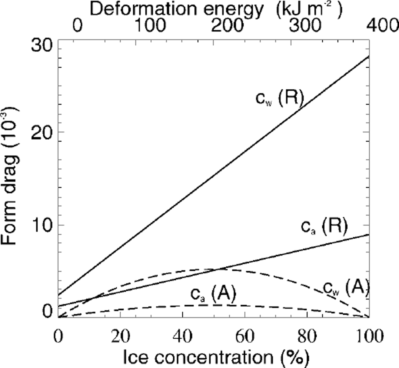
Atmospheric and oceanic drag coefficients are dependent on both roughness and stratification (e.g. Reference Overland and DavidsonOverland and Davidson, 1992; Reference Overland and ColonyOverland and Colony, 1994). In the NCEP/ NCAR re-analysis model, bulk aerodynamic formulas are used in the surface layer, where fluxes of sensible heat, moisture and momentum are proportional to the difference between values at the surface and in the adjacent atmosphere. The proportionality constants are dependent on wind speed and static stability of the surface layer (Reference KanamitsuKanamitsu, 1989). Therefore we assume that the appropriate stability parameterization is included in the analyses model and focus on the dependency on roughness. The surface-layer 10 m drag coefficient is a regional value of air-ice coupling which includes the influence of ridges and leads (Reference Overland and ColonyOverland and Colony, 1994). Models based on the continuity hypothesis cannot resolve single floes and leads. Therefore a universal formulation of drag coefficients depending on ice concentration and deformation energy is an appropriate method to account for the varying influence of form drag also in large-scale sea-ice models. Form drag is composed of two elements: ice surface roughness and floe edges. The first contribution increases with enhanced deformation and is therefore approximated by a function of deformation energy (Reference Steiner, Harder and LemkeSteiner and others, 1999). Reference Banke, Smith and AndersonBanke and others (1980) showed that the 10 m drag coefficient is linearly related to a measurable surface roughness parameter which is obtained from an integration of a snow-surface roughness spectrum. The second contribution varies in conjunction with concentration. Simulated ice concentration is in good correspondence with observed satellite passive-microwave-derived ice concentrations from Reference Gloersen, Campbell, Cavalieri, Comiso, Parkinson and ZwallyGloersen and others (1992). In winter an almost compact ice cover is visible in both simulation and observation. In summer, variations are of about 5−10% which is within the accuracy range of the satellite data. We therefore assume the ice concentration to be accurate enough to include in the parameterization. Previous works indicate that the atmospheric drag coefficient rises with increasing ice concentration, then falls at higher concentrations (Reference Andreas, Tucker and AckleyAndreas and others, 1984; Reference Guest and DavidsonGuest and Davidson, 1987). Observations of Reference Mai, Wamser and KottmeierMai and others (1996) show a maximum form-drag contribution for 50% ice coverage. With ongoing enhancement of the ice concentration, the contribution due to floe edges decreases until vanishing for 100% ice coverage. If there is no ice, the contribution is also zero. Reference Hartmann, Kottmeier, Wamser, Augstein, Johannessen, Muench and OverlandHartmann and others (1994) show a similar picture but they do not give any definite relation. In another formulation the oceanic and atmospheric drag coefficients are given as a combination of skin drag and form drag. Skin drag (10³bw = 1.2; 10³6_a = 0.8) is determined according to the lowest observed drag coefficients (e.g. Reference Shirisawa and AotaShirisawa and Aota, 1991; Reference Shirasawa and IngramShirisawa and Ingram, 1991; Reference Wamser and MartinsonWamser and Martinson, 1993), and form drag is parameterized as a function of deformation energy and ice concentration (Fig. 1). The latter is defined with a maximum for a = 0.5 and zero for a = 0 and a = 1.0 (a ∊ 0,1 = 0,100%):

Fig. 1.

Oceanic (c_w) and atmospheric (ca drag coefficients parameterized as a linear function of deformation energy r (top scaling, solid lines) combined with a square function of ice concentration a (bottom scaling, dashed lines).

r and a are derived from the prognostic budget equations:

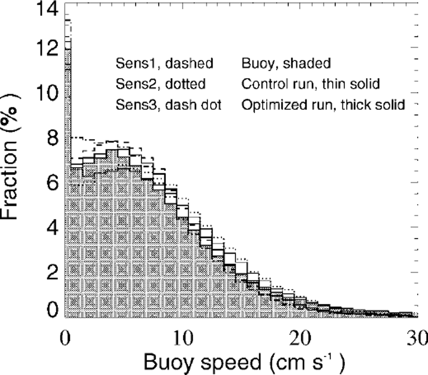
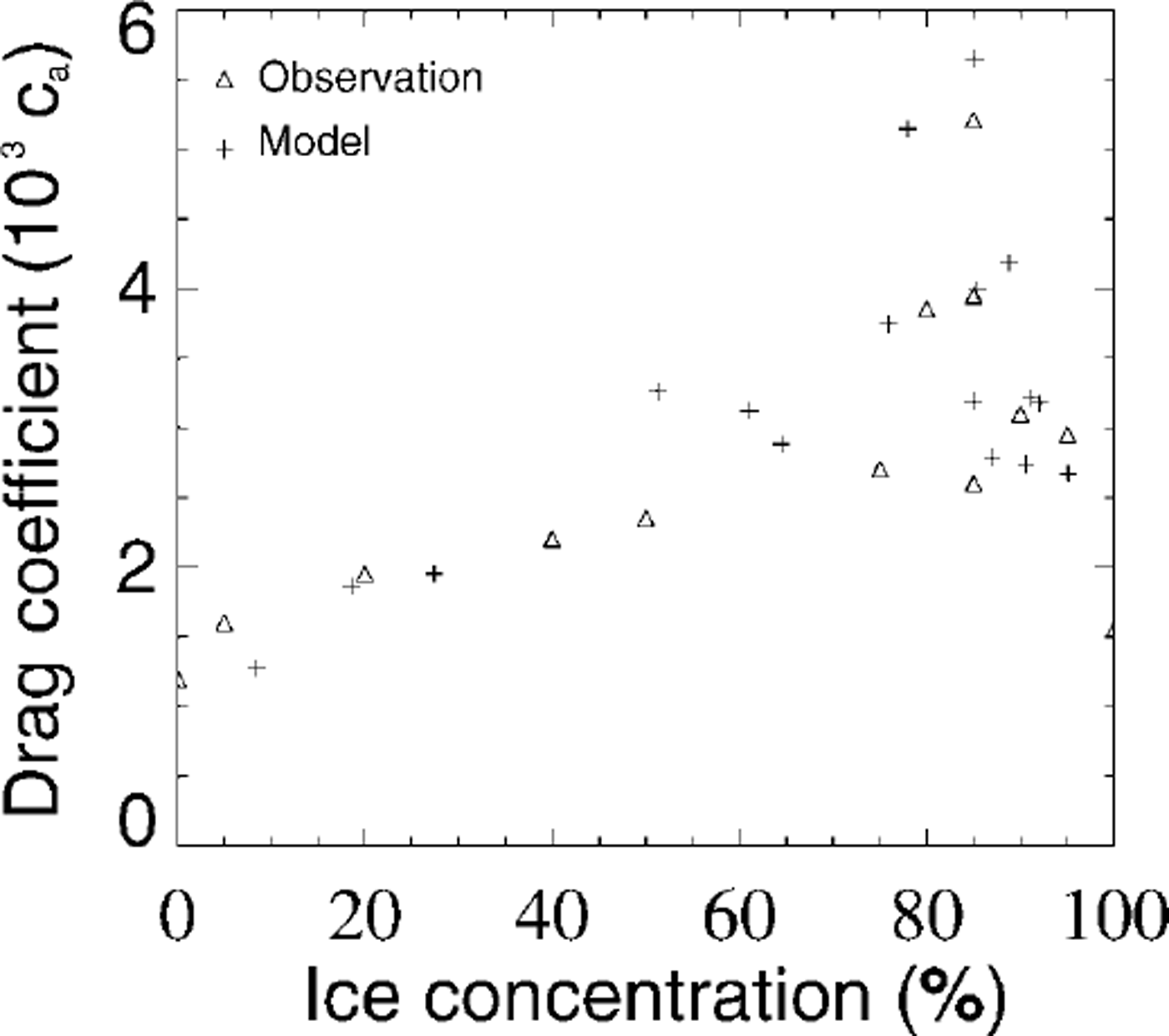
Thereby the lefthand sides have the form of a continuity equation and describe the local rates of change and advection. On the righthand sides source and sink terms are described, where s_a, after Reference HiblerHibler (1979) and Reference HarderHarder (1997), includes freezing, melting and lead formation due to shear forces and s_r includes melting and work by internal forces (Reference Steiner, Harder and LemkeSteiner and others, 1999). In a first approach the parameters m_a , m_w, d_a and dw are set referring to observed drag coefficient variations, then optimized via comparison with observed buoy-drift velocities to m_a = 1.9 × 10−⁸ m² J−¹, m_w = 6.0 × 10−8 m² J−¹, 103d_a = 1.3 and 10³ dw = 2.6. With the buoy data of the International Arctic Buoy Programme (IABP) (Reference Colony and RigorColony and Rigor, 1995), >100 000 daily drift velocities from 16 years (1979−94) are available. For the comparison with simulated drift velocities, only temporally and spatially corresponding data are used. Figure 2 shows velocity histograms for different sensitivity runs, which are used for the optimization. Sensl, with 10³ dw = 6.0, shows that an increase of d_w leads to an increase of the lower-velocity part and a slight decrease in the higher-velocity part. A decrease of dw shows inverse changes. Sens2, with m_w = 4.0 × 10−₈ m² J−¹, shows that a reduction of m_w leads to a reduction of the lower-velocity part and an increase in the mean velocity part, closer to the control run. An increase of m_w leads to unrealistically high deformation energies which in turn increase the drag coefficients. Sens3, with a reduction of m_a to 1.9 × 10"⁸ m² J−¹ leads to a distinct increase of the velocity part between 0 and 4 cm s−¹ and a reduction of larger velocities. (For the sensitivity runs, parameters not explicitly mentioned remain the same as in the optimized run.) In the control run the drag coefficients are set to the constant values c_w = 5.5 × 10−3 and c_a = 2.75 × 10−³, referring to the results of the Sea Ice Model Intercomparison Project (SIMIP). The steeper rise for the oceanic drag coefficient (Fig. 1) is conditioned by the stronger influence of keels on the oceanic boundary layer. Ridge keels are about four times the size of the corresponding sails, whereas the oceanic boundary layer is one-tenth the thickness of the atmospheric boundary layer. Figure 1 also indicates that the effect of form-drag contribution by ice concentration, compared to the total drag, is mainly important in regions with relatively low deformation energies (e.g. in the marginal ice zone and the Siberian shelf seas). For the comparison with observed drag coefficients it is necessary to view the complete drag coefficient parameterization, including concentration and roughness. Reference AndersonAnderson (1987) and Reference Guest and DavidsonGuest and Davidson (1987) show a maximum shifted towards higher concentrations, when grouping their measurements as a function of ice concentration. The same shift, as well as the slow increase and sharp decrease after reaching the maximum at 80−85%, can be seen in the simulation, plotting simulated drag coefficients c_a (A r) against the ice concentration at the respective gridpoints (Fig. 3). The square dependence on concentration, with maximum at 50%, which is, of course, only a first guess, reflects the pure dependence on concentration and cannot be compared independently to measurements representing a combined effect of roughness and concentration. (Reference AndersonAnderson (1987) recognizes large variations in drag coefficients for similar concentrations of 70−90% due to changes in roughness.) The observations in Figure 3 were recorded during the Marginal Ice Zone Experiment in July 1984 (MIZEX’84) in the East Greenland Sea (Reference AndersonAnderson, 1987). The respective model values are for July 1984 in approximately the same region (south of 82° N and between 5° Wand 25° E). A comparison of MIZEX’83 data (Reference Guest and DavidsonGuest and Davidson, 1987) with respective model results shows a similar good correspondence.

Fig. 2.

Velocity histograms for different sensitivity runs. observed buoy drift is shaded, control run with constant drag coefficients is indicated by a thin line and the optimized run, with variable drag coefficients as shown in figure 1, is indicated by a thick line. other lines show selected runs describing the variability of the velocity distributions due to parameter changes (see text).

Fig. 3.

Comparison of observed (triangle) and modelled (plus sign) neutral 10 m atmospheric drag coefficients grouped as a function of ice concentration. measurements are taken in the east greenland sea during mizex’84 (july 1984), reported in Reference Andersonanderson (1987). model data are for july 1984 in approximately the same region (south of 82° m and between 5° wand 25° e). parameterized drag coefficients (equation (3)) are plotted against the ice concentration at the respective gridpomts.

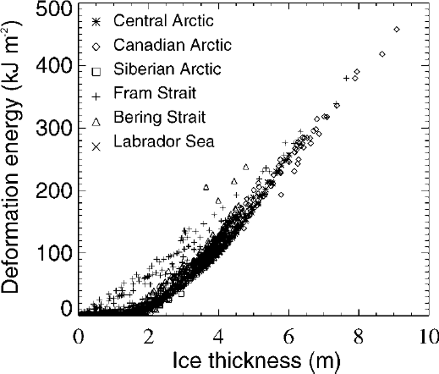
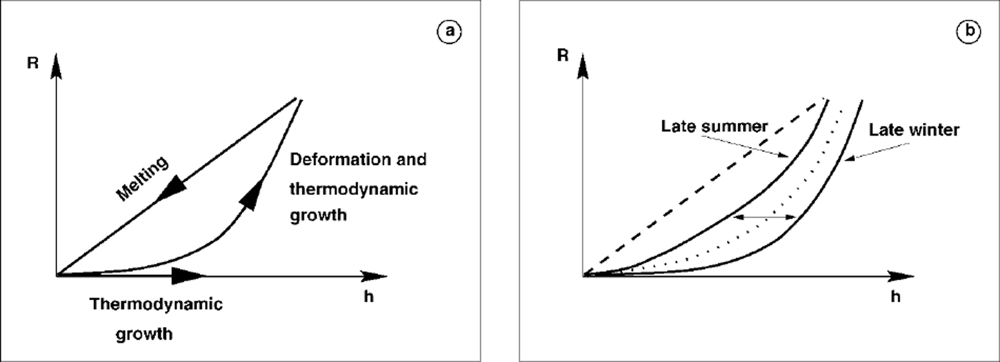
Sea-ice thickness is not included explicitly in the parameterization, because thermodynamic increase of thickness hardly changes the amount of momentum exchange. But, as Figure 4 indicates, simulated sea-ice roughness is closely related to ice thickness. The dynamic component of ice-thickness increase is already accounted for by the dependence on deformation energy. The relation in Figure 4 shows a sharp lower limit, which may be approximated by an exponential function r = a exp(bh) + c, where, for the control winter run, b ≈ 0.56 m−^{1 1}and and a a = - ^C ≈ 8.0 J m⁻². This means that a certain nil ice thickness is characterized by a minimum degree of deformation. The strongly regional subdivision also indicates that ice conditions may be characterized by their relation between thickness and deformation energy. The thought may occur that sea-ice roughness can be determined directly as, for example, an exponential function of sea-ice thickness. This is not totally excluded, but it needs to be remembered that, first, there is a division into a lower limit, determined by deformation and thermodynamic growth, and an upper limit, accounting for melting, which is a linear relation, by default in the model theory, and, second, the lower limit follows a seasonal cycle. Both points are illustrated in a schematic diagram (Fig. 5).

Fig. 4.

Comparison between simulated deformation energy r and thickness h in winter (1979−97) for different regions: central arctic (>85°n), siberian arctic ( <85° n, 45−135° e), fram strait ( <85° n, 135° e to 135° w), canadian arctic ( <85° n, 135−45° w), bering strait ( <85° n, 45° w to 45° e), labrador sea.

Fig. 5.

Schematic diagram of the relation between deformation energy r and ice thickness h. (a) the ascending branch describes the increase due to deformation and thermodynamic growth; the descending branch describes melting which is given as a linear relation betweenr and h. ( b) during the year the ascending branch shifts from higher thicknesses at the end of winter to lower thicknesses at the end of summer.

3. Results

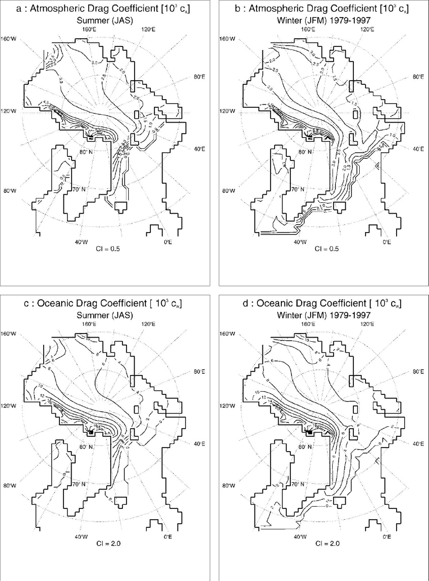
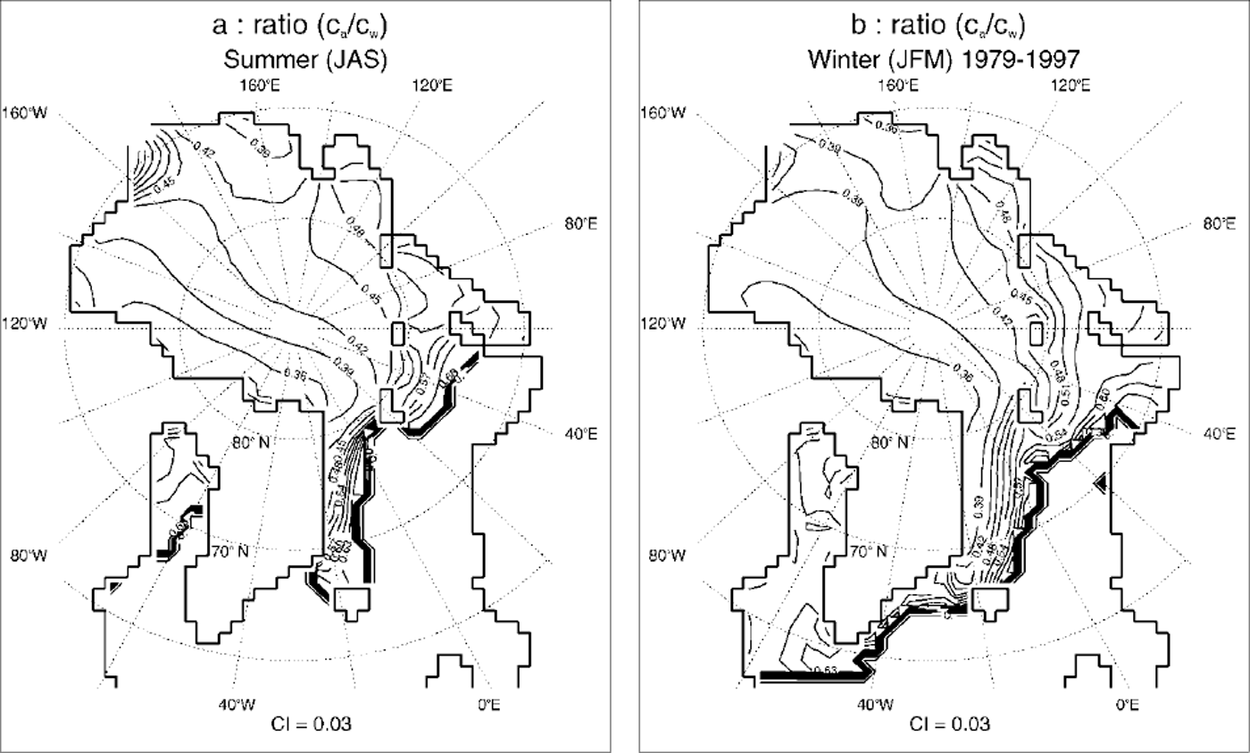
The formulation leads to temporally and spatially varying drag coefficients. Figure 6 shows respective summer and winter values, with low values in the regions with less deformed ice (Siberian shelf seas) and high values in regions with highly deformed ice (Canadian Archipelago, East Siberian Sea). Values in the North Pole region are about c_a = 2.5 × 10−³ and c_w = 6 × 10−³ in winter and c_a = 3.0 × 10−3 and c_w = 7 × 10−³ in summer. The rate of ocean drag is increased for higher deformed ice, as indicated by a reduced drag coefficient ratio Ca/cw of 0.36 and lower in the Canadian Archipelago and the East Siberian Sea, compared to values of up to 6.0 in the Barents, Kara and Laptev Seas (Fig. 7). Seasonal variability is mainly caused by changes in ice concentration, indicating that a large part of seasonal variability is an effect of floe-edge contribution. This may be explained by the fact that in summer, when relatively thin, smooth ice melts and breaks open, leads are built and the ice concentration reduces, while the pressure-ridge frequency recedes very slowly. In winter the influence of floe edges is mainly limited to the marginal ice zone, whereas ice coverage in the central Arctic is almost 100% and therefore form drag is mainly influenced by roughness elements (pressure ridges). Velocity histograms, divided up into different seasons, show a better fit of the optimized run to the observed buoy drift, especially for lower drift velocities (Fig. 8).

Fig. 6.

Simulated atmospheric drag coefficients (103ca) in (a) summer (july-september) and (b) winter (december-march), and simulated oceanic drag coefficients (103cw) in (c) summer and (d) winter, as a mean of 1979−97. contour intervals (ci) are 0.50 for the atmospheric drag coefficients and 2.00 for the oceanic drag coefficients.

Fig. 7.

Simulated ratio of atmospheric (ca) to oceanic (cw) drag coefficients in (a) summer (july-september) and (b) winter (december-march), as a mean of 1979−97. contour interval is 0.03.

Fig. 8.

Velocity histograms for buoy-drift (shaded), control (thin line) and optimized (thick line) run divided into different seasons.

Drag coefficent ratio variations result in local differences in amount and direction of the ice-drift velocity, which are highly variable. North of Greenland and in the outflow regions of the Siberian shelf seas, maximum values are ∼ 1 cm s−1 which is about one-third of the ∼3cm_S−1 maximum mean velocity in the respective regions. Ice stoppage northeast of Greenland, which has been somewhat too high in the SIMIP runs (personal communication from M. Kreyscher, 1999), is decreased, leading to higher ice-drift velocities in this region. Related export changes through Fram Strait and the Nordic Sea are of about 2% in the mean. Another effect of the parameterization is a reduction in keel frequency of about 1−2 per km in the East Siberian Sea, where, compared to Reference RomanovRomanov (1996), keel frequency was somewhat overestimated in the control run. Keel drafts and sail heights are also slightly reduced, leading to better agreement with observations from Reference RomanovRomanov (1996). In the Beaufort Sea a reduction is also visible, but Beaufort Sea keel frequencies and drafts are still overestimated, mainly because of missing outlets in the Canadian Archipelago due to the coarse land mask.

4. Conclusions

Drag coefficients are parameterized as a function of deformation energy and ice concentration, leading to a more accurate description of model dynamics due to regionally and spatially varying drag coefficients. The results show local differences of ice-drift velocities, ice thickness and deformation. The mean large-scale circulation pattern remains unchanged. Although improvements are visible, validation proves somewhat difficult because the effects of drag coefficient variations are partially hidden by larger model deficiencies: the model is still running with a constant ocean, so the variability of ocean drag is not adequately taken into account. Also the land mask in the Canadian Archipelago is too coarse, leading to an overestimation of thickness and deformation in the Beaufort Sea. For large-scale climate models where only the large-scale circulation is resolved, a parameterization as described may be meticulous, but for higher resolutions and on smaller (regional) scales a parameterization including form-drag variations is of major importance because small-scale effects will no longer be negligible.