1 Introduction
Flames are one of the most complex nonlinear dynamic systems, which involve the interplay between chemical reactions, heat and mass transfer, and flow dynamics (Sohn et al. Reference Sohn, Kim, Chung and Maruta2000; Kashinath, Waugh & Juniper Reference Kashinath, Waugh and Juniper2014). Since the eighteenth century, generations of scientists have devoted themselves to the study of flames, hoping to master the law of combustion and predict the evolution of practical flames. Even though considerable progress has been made due to the emergence of large-scale clusters and the development of computational fluid dynamics (CFD), online in situ prediction of 3-D flame evolution is still a formidable task (Kaminski et al. Reference Kaminski, Bai, Hult, Dreizler, Lindenmaier and Fuchs2000; Klein, Chakraborty & Ketterl Reference Klein, Chakraborty and Ketterl2017), mainly for two reasons: first, CFD modelling involves the solution of Navier–Stokes equations with millions or even billions of cells and thousands of time steps; second, a detailed chemical kinetic mechanism is only available for simple low-carbon fuels (Curran Reference Curran2019). In addition, since the CFD modelling is highly sensitive to boundary conditions – for example, the roughness and geometry of the boundary – this will cause extreme difficulties in practical applications where the boundary conditions are hard to define. Thus, the proposal and development of an alternative approach for 3-D flame prediction is of great interest.
Recently, time-resolved volumetric tomography (VT) for combustion diagnostics has made significant progress due to the invention of high-energy burst mode lasers and upgrades in high-speed cameras (Halls et al.
Reference Halls, Gord, Meyer, Thul, Slipchenko and Roy2017a
, Reference Halls, Hsu, Roy, Meyer and Gord2018). For example, volumetric imaging of important intermediate flame species such as OH,
 $\text{CH}_{2}\text{O}$
and PAH has been demonstrated with a repetition rate up to 10 kHz (Halls et al.
Reference Halls, Hsu, Jiang, Legge, Felver, Slipchenko, Roy, Meyer and Gord2017b
,Reference Halls, Jiang, Meyer, Roy, Slipchenko and Gord
c
). The development of VT has greatly facilitated understanding of complex combustion processes such as flame ignition and combustion instability (Ma et al.
Reference Ma, Lei, Wu, Xu, Ombrello and Carter2016; Ruan et al.
Reference Ruan, Yu, Chen, Wang, Cai and Lu2019). In addition, enormous amounts of experimental data can be accumulated within a short period of time. Such an amount of data provides unprecedented opportunities for machine learning (ML) algorithms which can effectively explore the hidden information behind the large dataset and make a faithful regression (Xu, Pei & Lai Reference Xu, Pei and Lai2017) or prediction (Bakkouri & Afdel Reference Bakkouri and Afdel2017). For example, in a recent review of developments in improving turbulence models by using ML algorithms it was proposed that data-driven approaches can be used to design useful predictive models (Duraisamy, Iaccarino & Xiao Reference Duraisamy, Iaccarino and Xiao2019). In particular, Kutz recommends that deep learning (DL) may play a key role in the field of fluid dynamics (Kutz Reference Kutz2017).
So far, successful applications of DL have been reported in various fields such as computer vision and speech recognition for its great ability to approximate complex functions of nonlinear systems (LeCun, Bengio & Hinton Reference LeCun, Bengio and Hinton2015). For example, convolution neural network (CNN) is famous for its capability in extracting features from images and has been applied extensively in medical imaging (Litjens et al.
Reference Litjens, Kooi, Bejnordi, Setio, Ciompi, Ghafoorian, van der Laak, van Ginneken and Sánchez2017), such as computed tomography (CT) and magnetic resonance imaging (MRI). In addition, DL algorithms had also been applied to predict heat release rates (Tóth, Garami & Csordás Reference Tóth, Garami and Csordás2017; Wang, Song & Chen Reference Wang, Song and Chen2017),
 $\text{NO}_{x}$
emission (Li et al.
Reference Li, Lu, Li and Yan2016) and oxygen contents (Yi, Yu & Chen Reference Yi, Yu and Chen2017) for combustion studies. Long short-term memory (LSTM) neural network (Hochreiter & Schmidhuber Reference Hochreiter and Schmidhuber1997) is one such algorithm that excels in predicting time series data, such as stock markets (Nelson, Pereira & Oliveira Reference Nelson, Pereira and Oliveira2017), weather forecasting (Qing & Niu Reference Qing and Niu2018) and simulated turbulent flows (Alathur Srinivasan Reference Alathur Srinivasan2018; Mohan & Gaitonde Reference Mohan and Gaitonde2018; Wang et al.
Reference Wang, Xiao, Fang, Govindan, Pain and Guo2018), to list a few. It has also been demonstrated for stance detection, where it has obtained state-of-the-art results (Augenstein et al.
Reference Augenstein, Rocktäschel, Vlachos and Bontcheva2016).
In this work, we aim to develop a data-driven approach to predict 3-D flame evolution, which combines the state-of-the-art VT technique with DL algorithms. The former can provide a tremendous amount of useful experimental data and the latter can effectively utilize this big data to construct efficient neural networks for prediction. Different from the CFD approaches, which start from the Navier–Stokes equations, here we start directly from experimental data of the target flame measured at previous time instants. The advantage is obvious – our method starts from true representations of the practical flame; however, this is not necessarily guaranteed by a CFD technique, as it depends on how accurate the flow model and the chemical kinetic mechanisms are, and how well the initial conditions can be characterized.
2 Volumetric tomography of 3-D flame imaging
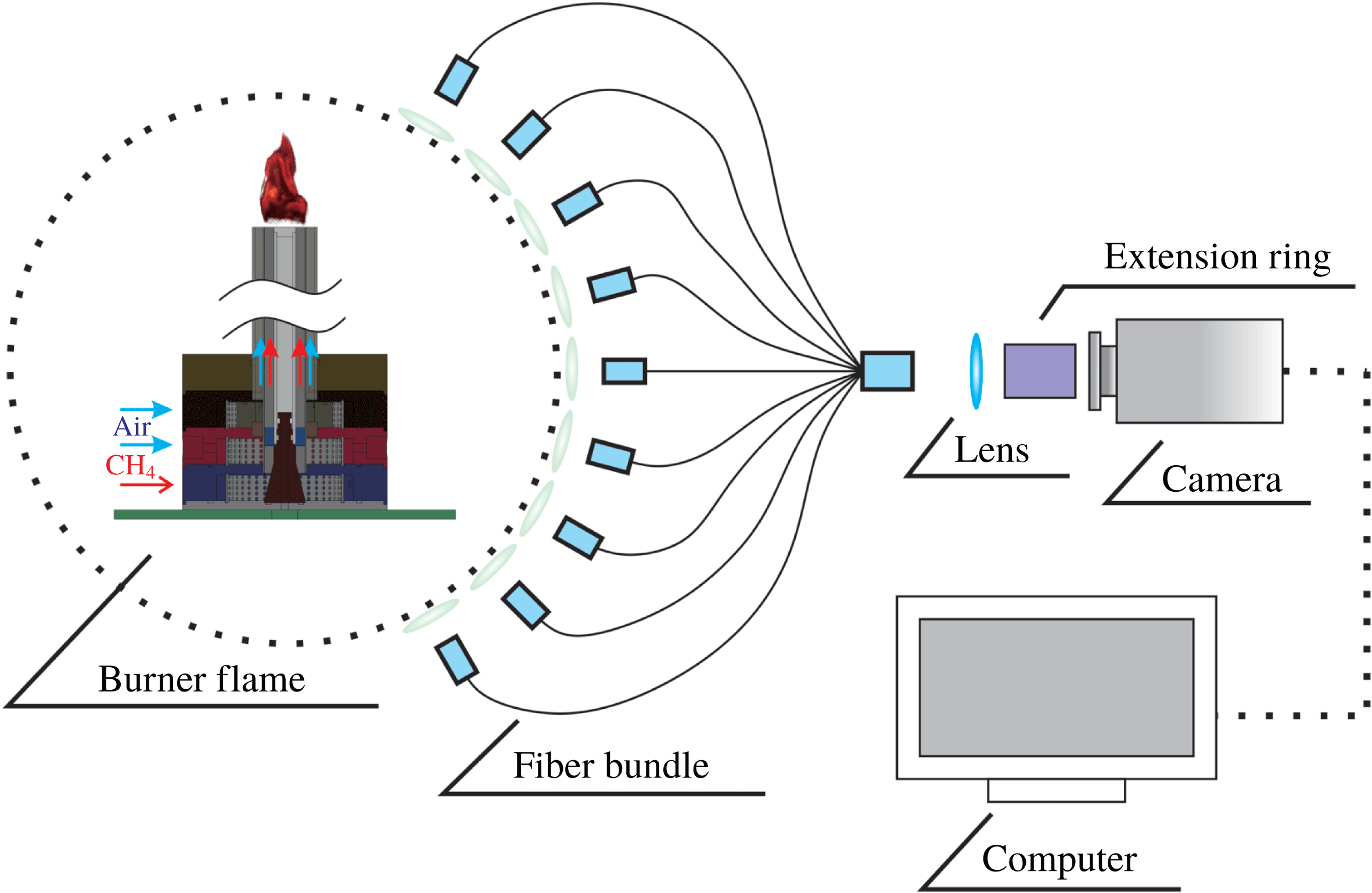
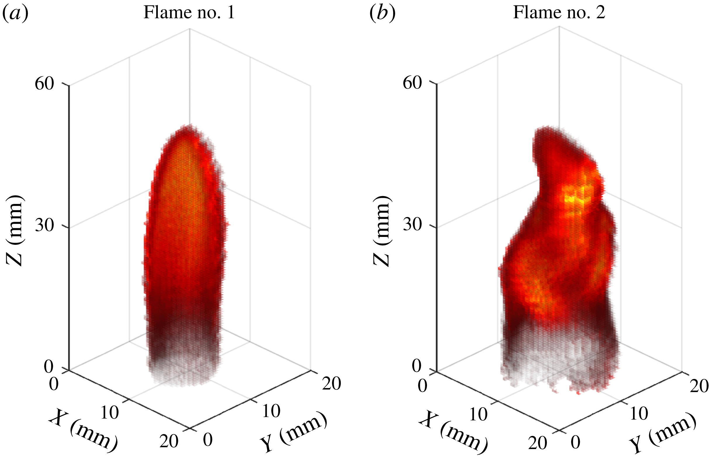
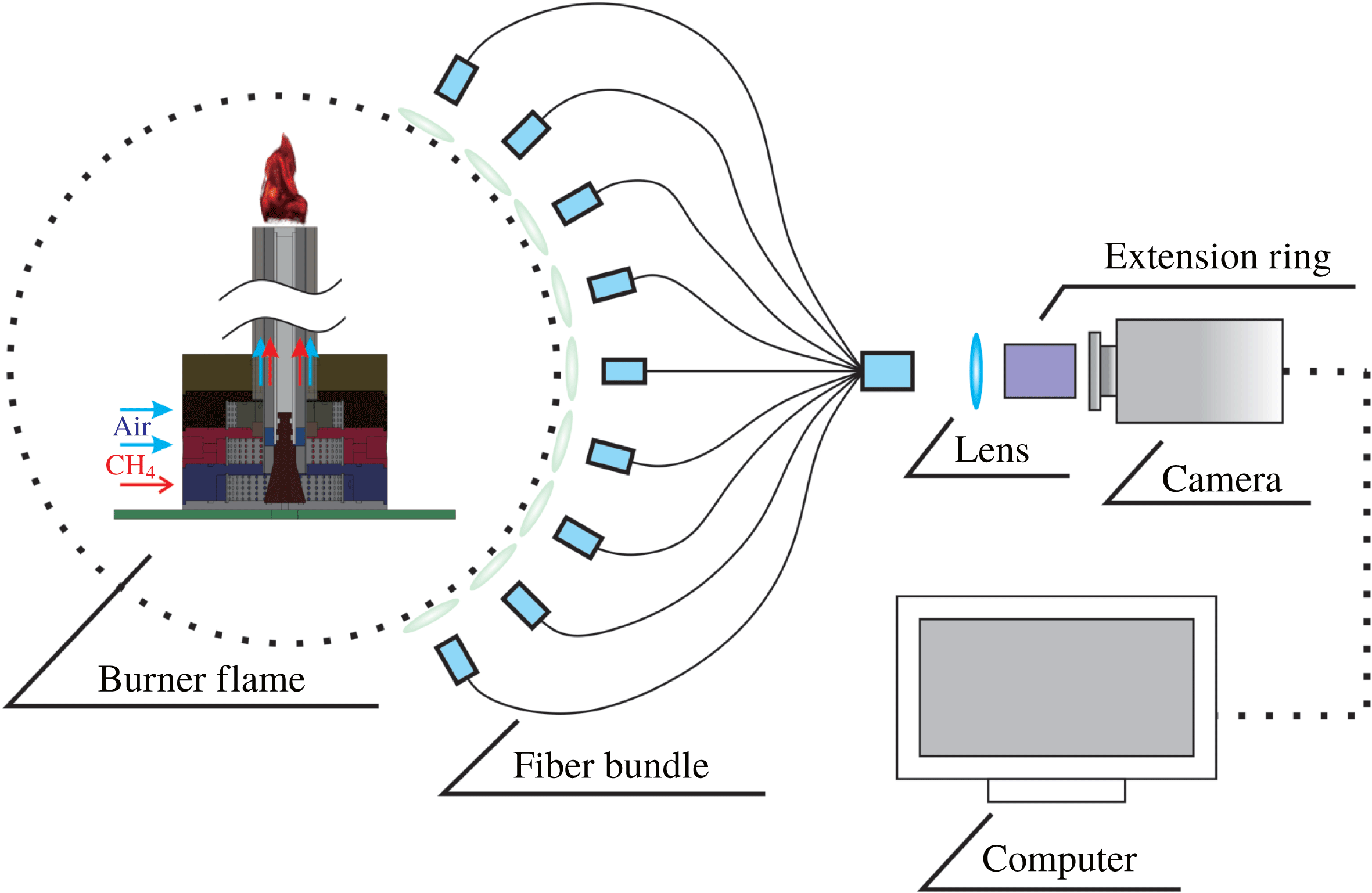
In this work, we designed a hybrid CNN–LSTM model to rapidly predict the evolution of 3-D flame structures based on its history 2-D projections without explicit tomographic reconstructions. Volumetric tomography of 3-D flame chemiluminescence was adopted here to generate a trustworthy dataset. The layout of the experimental set-up is shown in figure 1. Nine projections of the flame from different perspectives at each time instant were simultaneously captured by a camera through a customized fibre bundle which has nine input ends and one output end. The 3-D flame structures can then be reconstructed using the so-called algebraic reconstruction technique (ART) (Yu et al.
Reference Yu, Ruan, Liu, Cai and Lu2018). More details about the VT system, including the components of the set-up as well as the reconstruction process, can be found in the supplementary material available at https://doi.org/10.1017/jfm.2019.545. Capturing the projections continuously, for example, for 10 s with a framing rate of 1k and repeating the reconstruction processes, a dataset including 10 000 consecutive frames of the 3-D flame structures can be obtained. To test the CNN–LSTM model, both a simple laminar diffusion flame (Flame no. 1, see figure 2(a)) and a complex non-premixed turbulent swirl-stabilized flame (Flame no. 2, see figure 2(b)) were tested, which contain the main features of flame evolution, including changing flame heights, drifting of flame wrinkles and the rotation of flames. As shown in the movie (see supplementary material), the profile of both flames changed considerably over time. For both Flame no. 1 and Flame no. 2, the reconstruction volume was discretized into 50
 $\times$
50
 $\times$
110 voxels, with each voxel having dimensions of 0.5 mm
 $\times$
0.5 mm
 $\times$
0.5 mm.
Illustration of the volumetric tomography system, which consists of one swirl-stabilized burner, one customized fibre bundle, one high-speed camera and one computer. Nine projections from different angles are captured simultaneously and then used for the reconstruction of 3-D flame structures to generate both the training and testing datasets.
The 3-D renderings for Flame no. 1 and Flame no. 2.

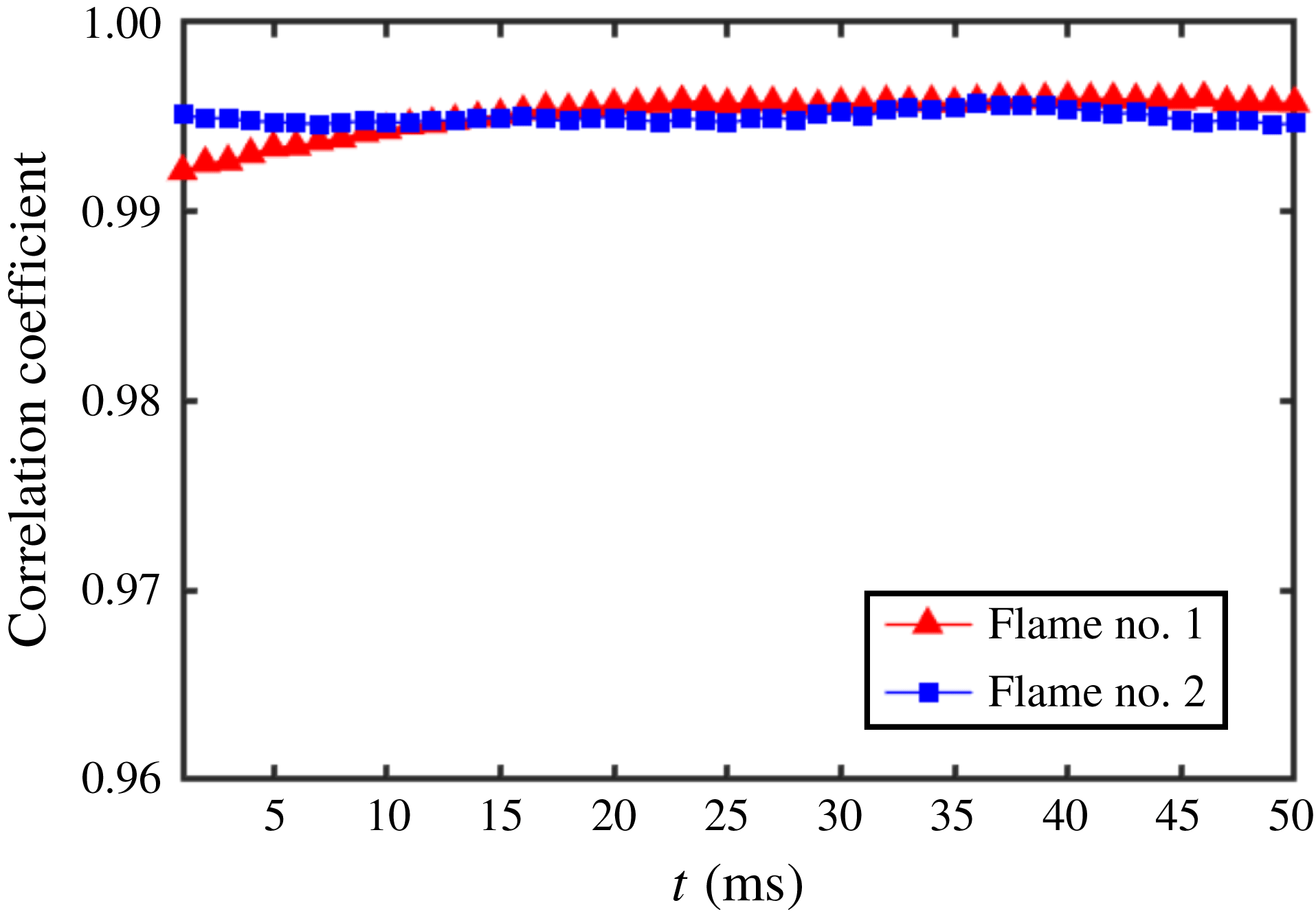
Correlation coefficients between the ninth measured projection and its corresponding re-projection, which are plotted as a function of the frame index of the two flames, respectively.

To validate the correctness of the reconstructions, the re-projection method was applied (Yu et al.
Reference Yu, Ruan, Liu, Cai and Lu2018). In this method, eight projections were used to reconstruct the 3-D flame structure, which was then used to predict the ninth projection. If the reconstruction is correct, then the estimate of the ninth projection should be consistent with the measured one. The correlation coefficient (R) between the estimate and the measurement of the ninth projection was used to quantify the quality of reconstructions. The definition of
 $R$
between two projections (
 $\boldsymbol{X}$
) and (
 $\boldsymbol{Y}$
) is (Shi, Liu & Yu Reference Shi, Liu and Yu2010)
 $$\begin{eqnarray}\displaystyle R(\boldsymbol{X},\boldsymbol{Y})={\displaystyle \frac{(\boldsymbol{X}\boldsymbol{\cdot }\boldsymbol{Y}^{\text{T}})}{\Vert \boldsymbol{X}\Vert _{2}\times \Vert \boldsymbol{Y}\Vert _{2}}}, & & \displaystyle\end{eqnarray}$$
where (
 $\cdot$
) represents the dot product between two vectors,
 $\Vert \cdot \Vert _{2}$
is the 2-norm of the vector and superscript T means the transpose of the row vector. As shown in figure 3, the correlation coefficients are constantly larger than 0.99 for the selected 50 frames of both flames, suggesting a good reconstruction accuracy of the VT system. Thus, the reconstructions of the flames using the ART algorithm can be considered as the ground truths and used to train and test our CNN–LSTM model.
3 Deep neural network
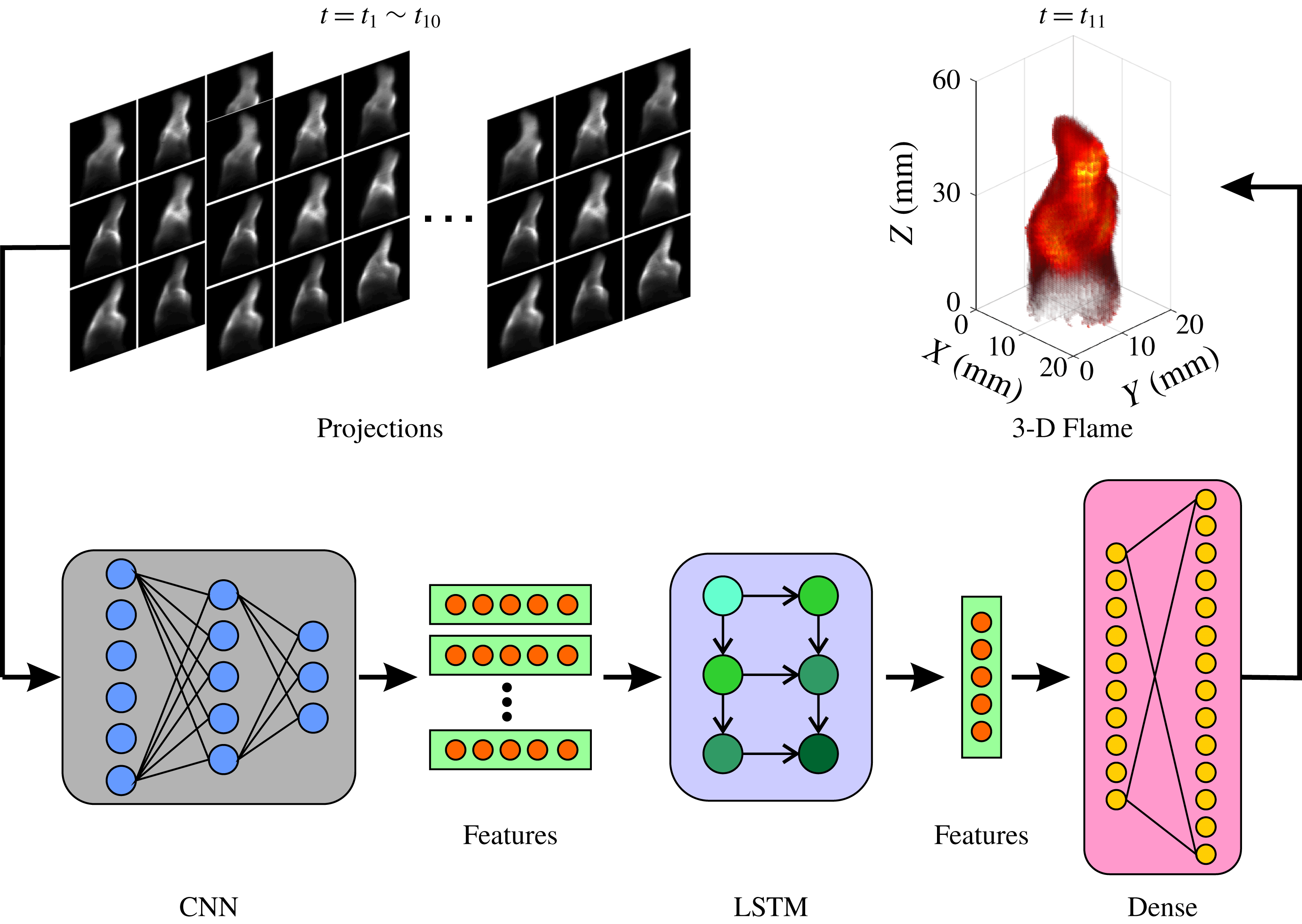
The evolution of a 3-D flame structure is essentially composed of translation, rotation, scaling, erosion and dilation of the structure. These operations are elemental for image processing and can be learned effectively with a deep learning algorithm. The schematic of our CNN–LSTM model is illustrated in figure 4. First, 10 000 samples obtained from the VT measurements, each of which contains nine projections and the corresponding 3-D flame structure, were divided into five groups to perform 5-fold cross-validation for our model. For example, the first four groups, containing 8000 samples (
 $t=0.001~\text{s}\sim 8.000~\text{s}$
), were used as the training dataset, and the last group, containing 2000 samples (
 $t=8.001~\text{s}\sim 10.000~\text{s}$
), was used as the testing dataset. The results presented below are the average results from the 5-fold cross-validation. The detailed frameworks of CNN and LSTM as well as the training strategies can be found in the supplementary material.
Schematic of the proposed CNN–LSTM model. The 3-D flame evolution (for example,
 $t=t_{11}$
) can be predicted based on its history 2-D projections (for example,
 $t=t_{1}\sim t_{10}$
) using this model, which comprises a convolutional neural network (CNN), a long short-term memory network (LSTM) and a dense layer.

It is noteworthy that the training process consists of two steps – training the CNN to extract features from projections, then training the LSTM to model the temporal sequence of these features. Within the iterations of the first step, nine projections at each time instant were put into CNN to obtain a vector of useful features. The 2-D projections for each frame can then be represented by the feature vector. Therefore, the problem of predicting the 3-D flame evolution can be transformed into another one of predicting the evolution of the corresponding feature vectors. Within the iterations in the second step, a sequence of history feature vectors (for example, at
 $t=t_{1}\sim t_{h}$
) and a future one (for example, at
 $t=t_{h+\unicode[STIX]{x0394}t}$
) were sent to the input layer and the output layer of the LSTM, respectively. The subscripts
 $h$
and
 $\unicode[STIX]{x0394}t$
denote history time window and prediction horizon, respectively. After 30 epochs, the loss function L2 converged and a trained CNN–LSTM prediction model was obtained. The details of the training process and the optimization of hyperparameters can be found in the supplementary material. Finally, the testing process was performed using the testing dataset. For instance, as shown in figure 4, projections (
 $t=t_{1}\sim t_{10}$
) in the testing dataset were input to the trained CNN–LSTM model to obtain the prediction of 3-D flame structure (
 $t=t_{11}$
), that is,
 $h=10~\text{ms}$
and
 $\unicode[STIX]{x0394}t=1~\text{ms}$
, which can be treated as one testing case.
4 Results
The neural networks were implemented, trained and tested using Keras (version 2.22.4) using the TensorFlow backend (version 12.112.0) in Python (version 32.62.8). All algorithms were implemented on a workstation equipped with an Intel® Core2™ i7-DMI2-X79 PHC 2
 $\cdot$
60 GHz CPU with a single NVIDIA TITAN XP GPU with 12 GB VRAM. The training process of the CNN–LSTM model took approximately 30 min and the computational cost for each prediction was approximately 2 ms without any specific code optimization. Thus, online in situ prediction of 3-D flame evolution can be achieved with a moderate coding effort by using multiple GPUs for parallel computing (You et al.
Reference You, Zhang, Hsieh, Demmel and Keutzer2017). Hence, our proposed method has an overwhelming advantage in terms of computational efficiency compared with CFD techniques.
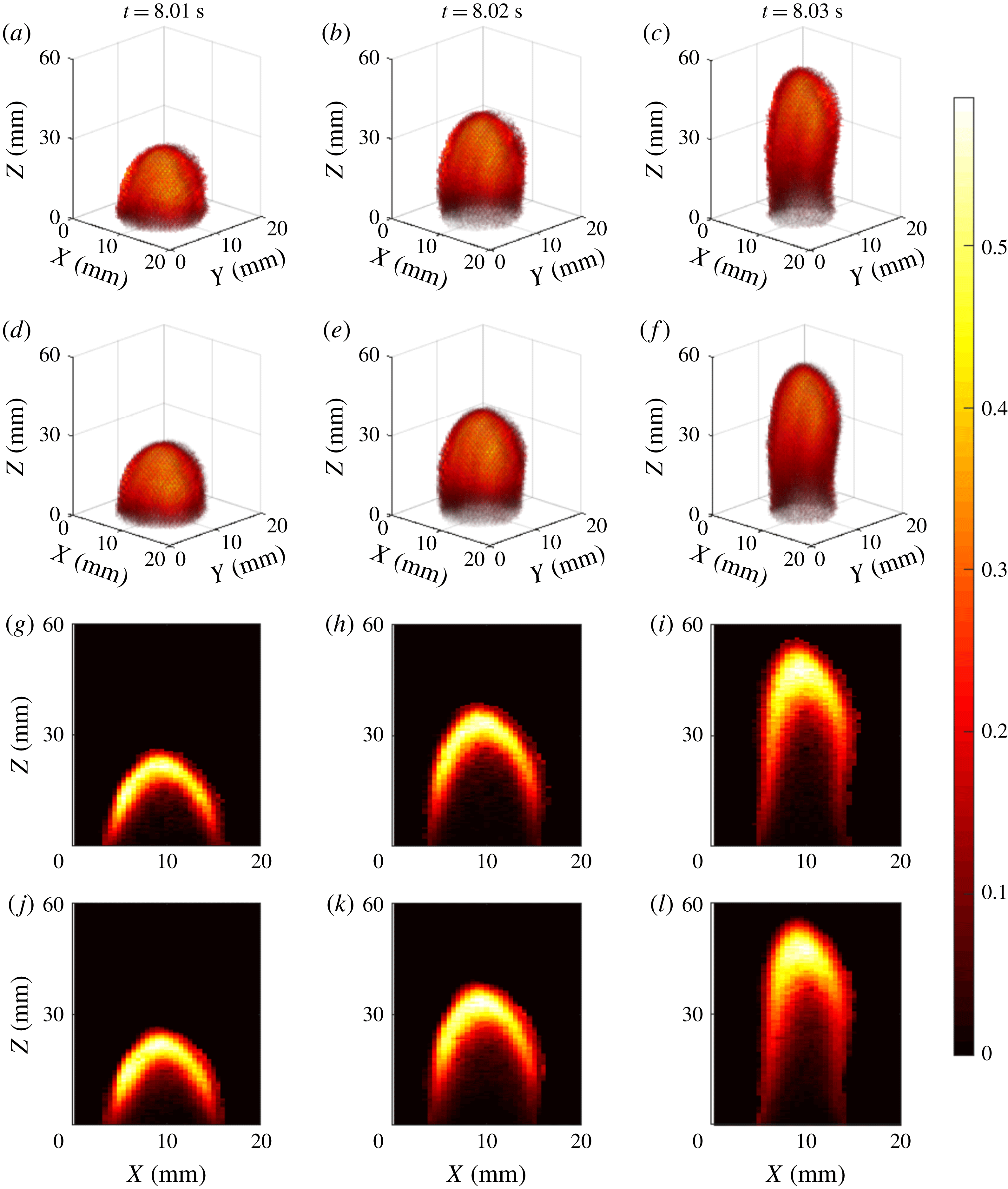
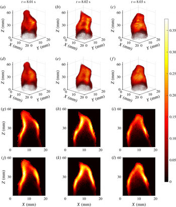
The testing results for three cases of both Flame no. 1 and no. 2 are shown in figures 5 and 6, respectively. As can be seen, there is almost no difference in the 3-D distributions between the ground truths (panels a–c) and the predictions (panels d–f), proving that our prediction model can successfully ‘learn’ the evolution law of flames and make accurate predictions. Furthermore, the middle slices of these 3-D distributions were selected to better illustrate the prediction performance of our proposed method, as shown in the last two rows of figures 5 and 6. As expected, the internal structures of both flames can be faithfully predicted as well. Thus, by using the CNN–LSTM model, the evolution of 3-D flame structures, including changing flame height, drifting of flame wrinkles and rotation of the flame, can be predicted accurately based on its history 2-D projections without explicitly tomographic reconstructions.
Prediction of Flame no. 1 using the CNN–LSTM model. Panels (a–c) are the ground truths at three time instants and panels (d–f) are the corresponding predictions obtained using the CNN–LSTM model. Panels (g–l) are the middle slices of panels (a–f), respectively.

Prediction of Flame no. 2 using the CNN–LSTM model. Panels (a–c) are the ground truths at three time instants and panels (d–f) are the corresponding predictions obtained using the CNN–LSTM model. Panels (g–l) are the middle slices of panels (a–f), respectively.

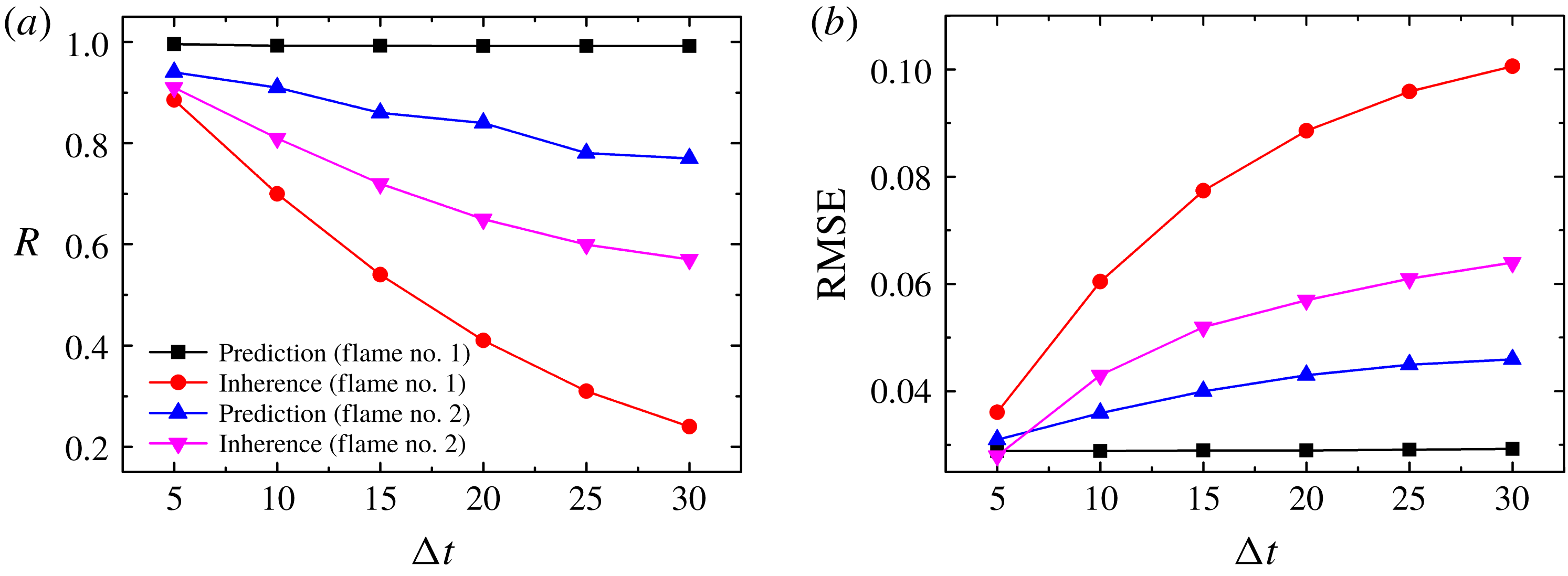
To further investigate the prediction capability of our CNN–LSTM model, several comparative experiments have been conducted with the same training and testing datasets. Quantitatively, the correlation coefficient (
 $R$
) and the root mean square error (RMSE) between the predictions and the ground truths were adopted as the performance parameters to evaluate prediction accuracy. The testing results as a function of prediction horizon (
 $\unicode[STIX]{x0394}t$
) are shown in figure 7. The values of
 $R$
and RMSE remained nearly constant for Flame no. 1 (black lines) and changed slightly for Flame no. 2 (blue lines), when
 $\unicode[STIX]{x0394}t$
increased from 5 ms to 30 ms. In contrast, the inherent
 $R$
and RMSE between two consecutive true frames (that is, the ground truths) with the same time interval (
 $\unicode[STIX]{x0394}t$
) were calculated as the basic benchmark. The results are shown in figure 7 (red and magenta lines for Flame no. 1 and Flame no. 2, respectively). Obviously, for the same
 $\unicode[STIX]{x0394}t$
, the inherent difference between two ground truths is much larger than the difference between the prediction and the ground truth for both Flame no. 1 and Flame no. 2, indicating the effectiveness of prediction.
Performance of CNN–LSTM model. The black and blue lines indicate the prediction performance (
 $R$
: correlation coefficient; RMSE: root mean square error) as a function of prediction horizon (
 $\unicode[STIX]{x0394}t$
) for both Flame no. 1 and Flame no. 2. The red and magenta lines denote the inherent
 $R$
and RMSE between two consecutive true frames (i.e. ground truths) with the same time interval (
 $\unicode[STIX]{x0394}t$
).

In addition, it has been found that the performance of the CNN–LSTM model varied for Flame no. 1 and Flame no. 2. This is mainly due to the distinct features of their structures and evolutions. Qualitatively, the evolution of Flame no. 1 was mainly reflected in the variation of the flame height, while the flame surface stayed relatively smooth over time. However, the height of Flame no. 2 was almost constant, but there were obvious wrinkles on the flame surface which drifted over time, making the flame structure more complicated. Its evolution is associated with vortex generation, movement and shedding. According to a relevant CFD study (Hasegawa, Nakamichi & Nishiki Reference Hasegawa, Nakamichi and Nishiki2002), small-scale vortices are more complex and irregular than large-scale vortices, and the evolution of Flame no. 2 was controlled by both scale vortices. To improve the prediction of Flame no. 2, more training samples should be incorporated so that more useful features of the small-scale vortices can be extracted, which is within the scope of our future research direction.
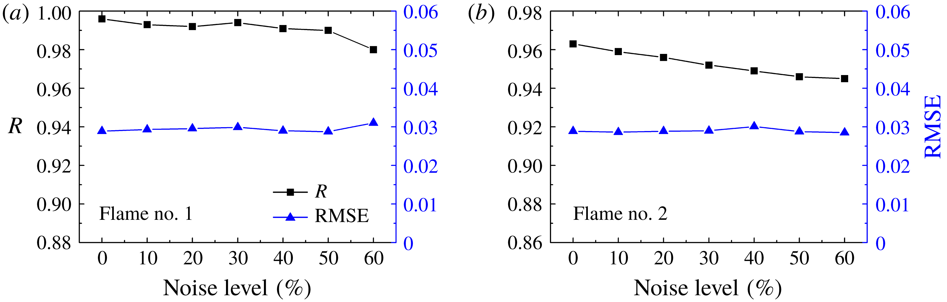
The successful demonstration of the CNN–LSTM model in predicting 3-D flame evolution suggested its potential for practical applications. In order to mimic the practical situations where measurement noise prevails, a series of experiments with different noise levels in projections were conducted. Additional artificial Gaussian noise was added to the measured projections as
 $$\begin{eqnarray}\displaystyle p^{\prime }=p\times (1+\unicode[STIX]{x1D6FF}\times g),g\sim G(0,1), & & \displaystyle\end{eqnarray}$$
where
 $p$
denotes the measured projections without noise,
 $\unicode[STIX]{x1D6FF}$
is the noise level and
 $g$
is a set of random numbers that satisfy a Gaussian distribution. The results shown in figure 8 suggested good noise immunity of the proposed CNN–LSTM model.
Results of experiments with different noise levels in projections. Additional artificial Gaussian noise was added to the measured projections to mimic the practical situations. Although the noise level increases gradually,
 $R$
decreases slightly and the RMSE remains nearly constant for both Flame no. 1 and Flame no. 2.

5 Summary
To summarize, a data-driven approach for the online in situ prediction of 3-D flame evolution based on volumetric tomography and deep learning algorithms has been proposed. The method was successfully demonstrated with proof-of-concept experiments by predicting the evolution of both a laminar diffusion flame and a non-premixed turbulent swirl-stabilized flame. There are two key advantages of this prediction model. First, the model starts directly from the experimental data of the target flame measured at previous time instants, which are true representations of the practical flames. Second, unlike CFD techniques, the solution of a complicated partial differential equation system is not required and only simple algorithmic operations are involved, resulting in an overwhelming advantage over CFD techniques in terms of computational efficiency. Thus, it serves as a promising alternative approach to CFD techniques for applications where rapid prediction of 3-D flame evolution is required. Although there was an implicit assumption that the dominant flame features of the training dataset and the testing dataset are similar (Noack, Morzyski & Tadmor Reference Noack, Morzyski and Tadmor2011), the prediction horizon can be effectively expanded when a larger training dataset is available. With the help of the proposed CNN–LSTM predictor, some key structure parameters of the flame (Floyd, Geipel & Kempf Reference Floyd, Geipel and Kempf2011) – such as flame surface density, wrinkling factor, flame normal direction and flame curvature, to name a few – can be calculated based on the predicted 3-D flame structures. Thus, these key parameters, which are related to flame stability and propagation (Floyd et al. Reference Floyd, Geipel and Kempf2011), can be used to control turbulent flames (Brunton & Noack Reference Brunton and Noack2015). Finally, the successful demonstration of our proposed model is just an example application of deep learning in predicting complex flows. It should be emphasized that this method can also be applied to predict the evolution of any other physical parameters/fields of reactive/non-reactive flows, such as the velocity field measured by particle image velocimetry (Baum et al. Reference Baum, Peterson, Surmann, Michaelis, Böhm and Dreizler2013) and the temperature field measured by two-line atomic fluorescence spectroscopy (Hult, Burns & Kaminski Reference Hult, Burns and Kaminski2005; Fang et al. Reference Fang, Zhang, Li, Tao, Wang, Hu and Song2019).
Acknowledgements
This work was funded by the National Natural Science Foundation of China under grant no. 51706141.
Supplementary movies
Supplementary movies are available at https://doi.org/10.1017/jfm.2019.545.