Introduction
Barley is grown throughout the world. Its production is mainly used as animal feed, with the remainder used for human consumption (groats and flakes) and for the production of alcohol (beer and malt). In 2023, the world area under barley amounted to about 146 million ha, while in the EU it was 47 million ha. According to FAOSTAT (2025), the main EU producers in 2023 were France (1.8 million ha) and Germany (1.6 million ha). In Poland, the corresponding area was 648 thousand ha (Statistics Poland, 2025). More than half of this area was planted with winter barley varieties.
Before new varieties of major crops, including winter barley, are recommended for cultivation, they are evaluated in a series of trials. First, they undergo plant breeding trials, followed by value-in-cultivation-and-use (VCU) trials, and finally post-registration trials. Plant breeders and crop experts then assess the stability and adaptability of new promising lines or varieties based on the results of these trials. The most common definition of ‘adaptability of a variety’ is its ability to demonstrate a high level of adaptation to diverse environments (Tigerstedt, Reference Tigerstedt1994). Two types of adaptability can be distinguished: wide and specific. Wide adaptation means that a variety performs well in nearly all environments, whereas specific adaptation means a variety that performs well in a subset of environments within a target region. A variety’s adaptability is assessed in relation to other genotypes and tends to change when better-performing varieties become available. The stability of a variety in terms of a given trait refers to its ability to perform consistently across a wide range of environments. Two concepts of stability are considered in the literature: static and dynamic (Becker and Leon, Reference Becker and Léon1988). Static stability means that a variety maintains constant values of a given trait across environments, while dynamic stability implies a stable variety response in each environment that is always parallel to the mean response of the tested varieties. The literature contains a number of proposals for stability measures. Recently, Pour-Aboughadareh et al. (Reference Pour-Aboughadareh, Khalili, Poczai and Olivoto2022) provided an overview of stability measures and their implementation in different statistical packages. The most popular are the Finlay-Wilkinson model (Finlay and Wilkinson, Reference Finlay and Wilkinson1963), the Eberhart and Russell model (Eberhart and Russell, Reference Eberhart and Russell1966), the ecovalence index (Wricke, Reference Wricke1962) or the additive main effects and multiplicative interaction model (Gauch, Reference Gauch1992). However, with the advancement in computational capabilities of computers, a mixed model approach has gained prominence (see e.g. Banaś et al., Reference Banaś, Przystalski and Łacka2023; Craine et al., Reference Craine, Choi, Schroeder, Brueggeman, Esser and Murphy2023; Laidig et al., Reference Laidig, Drobek and Meyer2008; Valenzuela-Antelo et al., Reference Valenzuela-Antelo, Benitez-Riquelme, Vargas-Hernandez, Huerta-Espino, Bentley, Villasenor-Mir and Pinera-Chavez2023; Piepho, Reference Piepho1999; Skovbjerg et al., Reference Skovbjerg, Knudsen, Füchtbauer, Stougaard, Stoddard, Janss and Andersen2020; Studnicki et al., Reference Studnicki, Paderewski, Piepho and Wójcik-Gront2017; and references therein). Piepho (Reference Piepho1999) demonstrated that the most prevalent models can be delineated through the utilisation of suitable covariance matrices for random effects. He also concluded that the problem of choosing the stability measure is equivalent to the problem of choosing the best model to describe the data (see also Piepho and van Eeuwijk, Reference Piepho, van Eeuwijk and Kang2002; Studnicki et al., Reference Studnicki, Paderewski, Piepho and Wójcik-Gront2017; Banaś et al., Reference Banaś, Przystalski and Łacka2023).
Stability analyses are commonly conducted on two-way variety
 $ \times $
environment data (see e.g. Banaś et al., Reference Banaś, Przystalski and Łacka2023; Craine et al., Reference Craine, Choi, Schroeder, Brueggeman, Esser and Murphy2023; Kurasiak-Popowska et al., Reference Kurasiak-Popowska, Katańska-Kaczmarek, Matysik, Stefański, Przybył, Skotarczak and Nawracała2024; Piepho and van Eeuwijk, Reference Piepho, van Eeuwijk and Kang2002; Studnicki et al., Reference Studnicki, Paderewski, Piepho and Wójcik-Gront2017; Valenzuela-Antelo et al., Reference Valenzuela-Antelo, Benitez-Riquelme, Vargas-Hernandez, Huerta-Espino, Bentley, Villasenor-Mir and Pinera-Chavez2023, and the references therein). However, analyses performed on three-way variety
 $ \times $
year
 $ \times $
location data are less frequent. Caliński et al. (Reference Caliński, Czajka and Kaczmarek1987a,b) used a two-stage approach and evaluated the stability of 10 wheat varieties using a multivariate model. In this model, they treated variety effects as fixed, while the rest was treated as random. In addition, they assumed that all trials were organised in a randomised complete block design. Czajka (Reference Czajka1995) extended these results by relaxing the assumption about the design of the experiment. He assumed that all trials were organised in the same block design. Piepho and van Eeuwijk (Reference Piepho, van Eeuwijk and Kang2002) also analysed a three-way data set in order to identify the most stable variety. In this study, the random effects were grouped into three categories: variation between years; variation between locations; and the interaction between year and location. Furthermore, different covariance matrices for each group were given consideration. In a different study, Skovbjerg et al. (Reference Skovbjerg, Knudsen, Füchtbauer, Stougaard, Stoddard, Janss and Andersen2020) investigated the stability and adaptability of 17 faba bean varieties. They assessed the varieties’ adaptability using a linear mixed model that included a cultivar-specific linear term as the product of the cultivar-specific regression coefficient and the environmental mean yield. They used the coefficient of variation to evaluate the stability of the varieties. In the current study, generalised stability variance (Piepho, Reference Piepho1994) was used as a stability measure. This stability measure is an extension of Shukla’s stability variance (Shukla, Reference Shukla1972), which is a function of
 $\sigma _{GL,i}^2$
,
 $\sigma _{GY,i}^2$
and
 $\sigma _{e,i}^2$
. Piepho (Reference Piepho1994) argued that a reliable assessment of stability, including the genotype × year interaction, requires ten or more years of testing. However, this is not feasible in most VCU trials, since by the time sufficient data have been compiled, the varieties under consideration will likely have been withdrawn from trials or removed from the NL list. Furthermore, some varieties may have zero estimates for the variance components
 $\sigma _{GL,i}^2$
or/and
 $\sigma _{GY,i}^2$
. Therefore, a Bayesian approach was used.
In this study, we fitted a Bayesian hierarchical model with variety-by-year, variety-by-location and residual variety-specific variances in order to evaluate the stability and adaptability of barley varieties. For comparison, we also fitted a Bayesian hierarchical model that included only residual variety-specific variances. One useful feature of a Bayesian approach is the ability to use prior information or expert knowledge. This subjective approach involves defining prior probabilities for unknown parameters based on personal experience and judgment. It recognises that expert opinion is better than having no knowledge. Nonyane and Theobald (Reference Nonyane and Theobald2008) used expert knowledge to construct informative priors for variance components. However, since plant breeders and variety offices possess long-term data, the hyperparameters can be updated, as can the knowledge regarding the variance components (see e.g., Laidig et al., Reference Laidig, Drobek and Meyer2008). Singh et al. (Reference Singh, Al-Yassin and Omer2015) and Studnicki and Piepho (Reference Studnicki and Piepho2024) presented methods for combining information on variance component estimates from previous trials to construct informative priors. In the current study, estimates of variance components were available from previous studies. To construct reliable scale parameters for the variance components, we first reanalysed the previous datasets and expressed the standard deviation estimates on a log scale. Next, we performed a meta-analysis of these logarithms to combine information from the previous studies. Furthermore, Theobald et al. (Reference Theobald, Talbot and Nabugoomu2002) noted that a Bayesian approach can address the issue of estimating complex mixed models for which the variance component is zero. Additionally, this approach provides an opportunity to estimate new quantities that are functions of model parameters. In this study, adaptability was assessed using the relative genotypic performance value index, which is based on posterior genotypic value estimates from the best model (see Pour-Aboughadareh et al., Reference Pour-Aboughadareh, Khalili, Poczai and Olivoto2022, and references therein). Lastly, selecting the best lines in plant breeding trials or varieties in a series of VCU field trials can be considered a decision-making problem under uncertainty. Therefore, we used a Bayesian probabilistic approach to facilitate the decision-making process for variety recommendations. We supplemented our stability analyses by calculating the probabilities of superior performance and the pair-wise probabilities for the ge variances. For each variety, we also calculated the joint probability of superior performance and stability (Dias et al., Reference Dias, dos Santos, Krause, Piepho, Guimarães, Pastina and Garcia2022). However, in contrast to Dias et al. (Reference Dias, dos Santos, Krause, Piepho, Guimarães, Pastina and Garcia2022), we calculated these probabilities without assuming independence between the two events. The first consideration of probabilistic concepts to support variety recommendation was by Mead et al. (Reference Mead, Riley, Dear and Singh1986). These concepts were subsequently developed further by Eskridge and Mumm (Reference Eskridge and Mumm1992), Piepho (Reference Piepho1996) and Piepho and van Eeuwijk (Reference Piepho, van Eeuwijk and Kang2002). In all of these studies, the authors made the assumption that yields were normally distributed across environments when calculating probabilities. In the Bayesian setting, Dias et al. (Reference Dias, dos Santos, Krause, Piepho, Guimarães, Pastina and Garcia2022) were the first to consider probability concepts for cultivar recommendations in multi-environment trials. Similar concepts were also utilised by Przystalski and Lenartowicz (Reference Przystalski and Lenartowicz2023). However, in that study, they only calculated the probability of superior performance for each variety. Miranda et al. (Reference Miranda, Dias, Júnior, Carneiro, Carneiro, Carneiro, Souza, Melo, Pereira, Vieira and Martins2024) applied the Bayesian probabilistic method to recommend common bean varieties, using a two-way genotype-environment table. In a different study, Chaves et al. (Reference Chaves, Krause, Dias, Garcia and Dias2024) demonstrated the application of the Bayesian probabilistic method to two- and three-way datasets. As in Miranda et al. (Reference Miranda, Dias, Júnior, Carneiro, Carneiro, Carneiro, Souza, Melo, Pereira, Vieira and Martins2024) and Chaves et al. (Reference Chaves, Krause, Dias, Garcia and Dias2024), all probabilities in this study were calculated using MCMC samples from the Bayesian analysis.
The current study aimed to show an application of a Bayesian hierarchical model with variety-by-year, variety-by-location and residual variety-specific variances in order to evaluate the stability and adaptability of barley varieties. For comparison, we fitted a Bayesian hierarchical model that included only residual variety-specific variances. As in Sorensen and Waagepetersen (Reference Sorensen and Waagepetersen2003) and Yang et al. (Reference Yang, Schön and Sorensen2012), we used the regression approach to model heterogeneity in Bayesian linear mixed models. Additionally, we show how the Bayesian probabilistic approach can facilitate the decision-making process for variety recommendations. To illustrate the proposed approach, we used the results of barley post-registration trials conducted in the 2020/21, 2021/22, and 2022/23 growing seasons.
Materials and methods
Data
This study analysed a subset of variety means (expressed in t/ha) from a series of field trials with winter barley conducted during the 2020/21, 2021/22 and 2022/23 growing seasons. The winter barley trials were planned in GL designs with two rows (two replicates), which were next split longwise and half of each row (replicate) was treated with additional fertiliser and was chemically protected (high-input). So in result, the incomplete split-block design was used. (Pilarczyk, Reference Pilarczyk2009). Recommendations for farmers from post-registration trials are issued mainly on the basis of the results of basic management intensity. Therefore, the results from this level of crop management intensity were used in the current study. In each growing season, trials were conducted at 32 experimental sites owned by the Research Centre for Cultivar Testing (COBORU). A complete list of the sites used and the years they were used is provided in Supplement S1. Figure 1 shows the locations of the experimental sites.
Locations of the experimental sites where the trials were conducted.

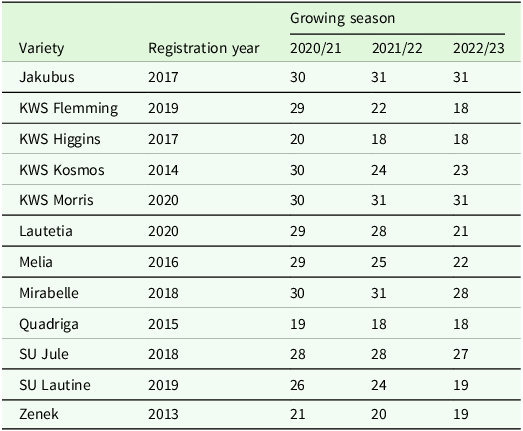
As shown in Supplement S1, approximately 30 varieties were tested in each growing season. In the present study, the stability and adaptability of the varieties tested over three growing seasons (though not necessarily at all sites) was assessed. The list of varieties included in this study, along with their registration year, is given in Table 1. The numbers presented in the final three columns of Table 1 indicate the number of sites in which a given variety was tested in a given growing season. The imbalance of the dataset has been shown using a heat map (Figure 2), in which the data in Table 1 are expressed as a percentage of the sites at which a given variety was tested in a given growing season.
List of varieties included in the study with their registration year and the number of sites in which a given variety was tested in a given growing season

Heatmap showing the imbalance of the dataset.

Except for two varieties (Quadriga and Zenek) which are of French origin, all the other varieties were bred in Germany. Most of varieties were registered in the years 2018-2020. The oldest variety was registered in 2013.
Statistical estimation
The mean yields (
 ${y_{ijk}}$
) were modelled with two Bayesian models. In the baseline model (called M1) it was assumed that
 ${y_{ijk}}$
has conditional normal likelihood, defined as follows:
 $${y_{ijk}}|{\mu _j},{u_i},{v_k},{t_{ij}},{w_{ik}},{z_{jk}}\sim N\left( {E\left( {{y_{ijk}}} \right),\sigma _i^2} \right)$$
where
 $$E\left( {{y_{ijk}}|{\mu _j},{u_i},{v_k},{t_{ij}},{w_{ik}},{z_{jk}}} \right) = {\mu _j} + {u_i} + {v_k} + {t_{ij}} + {w_{ik}} + {z_{jk}}$$
 $\;E( \cdot | \cdot )$
denotes the conditional expected value,
 ${\mu _j}$
is the mean of
 $j$
-th year (
 $j = 1,2, \ldots, \;J$
),
 ${u_i}$
is the effect of the
 $i$
-th variety (
 $i = 1,2, \ldots, \;I$
), and
 ${v_k}$
is the effect of the
 $k$
-th site (
 $k = 1,2, \ldots, \;K$
). By
 ${t_{ij}}$
,
 ${w_{ik}}$
,
 ${z_{jk}}$
we denoted in (2) variety-by-year interaction, variety-by-site interaction, and year-by-site interaction, respectively.
For annual means
 ${\mu _j}$
we assigned a normal distribution with mean
 ${m_j}$
and variance
 $r_j^2$
. i.e.
 $${\mu _j}\sim N\left( {{m_j},r_j^2} \right)$$
The prior distribution for each effect in model M1 was defined as follows:
 $${u_i}\sim N\left( {0,\sigma _u^2} \right)$$
 $${v_k}\sim N\left( {0,\sigma _v^2} \right)$$
 $${t_{ij}}\sim N\left( {0,\sigma _{{t_i}}^2} \right)$$
 $${w_{ik}}\sim N\left( {0,\sigma _{{w_i}}^2} \right)$$
 $${z_{jk}}\sim N\left( {0,\sigma _z^2} \right)$$
where
 $N\left( {0,\sigma _l^2} \right)$
represent normal distribution centered at zero and variance
 $\sigma _l^2$
(
 $l = u,v,{t_i},{w_i},z;i = 1, \ldots, I$
).
In order to finalise the specification of model M1, it is necessary to specify prior distributions for variance components. For the variance components
 $\sigma _l^2$
(
 $l = u,v,z$
), we assumed scaled-inverse-
 ${\chi ^2}$
(
 $IC$
) distributions with scale parameters
 $s_l^2$
and
 ${p_l}$
degrees of freedom, i.e.
 $\sigma _l^2\sim IC\left( {s_l^2,{p_l}} \right)$
, (
 $l = u,v,z$
). Increased degrees of freedom are associated with greater confidence in prior estimates
 $s_l^2$
. Equivalently, if
 $IG\left( {\gamma, \delta } \right)$
denotes inverse-Gamma distribution, then the
 $\sigma _l^2$
have an inverse-Gamma distribution
 $IG\left( {{{{p_l}} \over 2},{{{p_l}s_l^2} \over 2}} \right)$
. The residual variances, denoted by
 $\sigma _i^2$
, were modelled using a generalised linear model framework with a natural log link function (see e.g. Sorensen and Waagepetersen, Reference Sorensen and Waagepetersen2003; Yang et al. Reference Yang, Schön and Sorensen2012; and the references therein):
 $${\rm{log}}\left( {\sigma _i^2} \right) = a + {g_i}$$
where
 $a$
is an unknown scalar parameter and
 ${g_i}$
is variety effect on the natural logarithm of error variances. The parameter
 $a$
defines some kind of average variance across all genotypes, years and sites, while the effect
 ${g_i}$
describes the extent to which residual variance tends to be higher for observations of the
 $i$
-th variety. The term
 ${\rm{exp}}\left( a \right)$
can be treated as an unobserved marginal or ‘mean’ residual variance across all varieties, years, and sites. The term
 ${\rm{exp}}\left( {a{\rm{\;}} + {\rm{\;}}{g_i}} \right)$
can be interpreted as the error variance across a random sample of years and sites for variety
 $i$
. can be interpreted as the error variance across a random sample of years and sites for variety
 $i$
. To complete the model specification for
 $\sigma _i^2$
, we assumed that
 $a\sim N\left( {0,100} \right)$
,
 ${g_i}\sim N\left( {0,\sigma _g^2} \right),$
while the variance component
 $\sigma _g^2$
was given inverse-Gamma distribution with parameters 1 and 0.01, i.e.
 $\sigma _g^2\sim IG\left( {1,0.01} \right)$
. The same approach was used to model
 $\sigma _{{t_i}}^2$
and
 $\sigma _{{w_i}}^2$
, i.e. we assumed that
 $${\rm{log}}\left( {\sigma _{{t_i}}^2{\rm{\;}}} \right) = b + {d_i}$$
and
 $${\rm{log}}\left( {\sigma _{{w_i}}^2{\rm{\;}}} \right) = c + {f_i}$$
To complete the model specification for
 $\sigma _{{t_i}}^2$
and
 $\sigma _{{w_i}}^2$
, we assumed that
 $b,c\sim N\left( {0,10} \right)$
,
 ${d_i}\sim N\left( {0,\sigma _d^2} \right)$
,
 ${f_i}\sim N\left( {0,\sigma _f^2} \right),$
while the variances
 $\sigma _r^2$
(
 $r = d,f$
) were given inverse-Gamma distribution with parameters 1 and 0.1, i.e.
 $\sigma _r^2\sim IG\left( {1,0.1} \right).$
In the second model (M2) we assumed that
 ${t_{ij}}\sim N\left( {0,\sigma _t^2} \right)$
and
 ${w_{ik}}\sim N\left( {0,\sigma _w^2} \right)$
. Further, we assumed that
 $\sigma _l^2\sim IC\left( {s_l^2,{p_l}} \right)$
,
 $l = t,w$
. Other parts of the model are as previously defined in model M1.
In the two models under consideration, the variety means were computed as follows:
 $$M{V_i} = M + {\hat \alpha _i}$$
where
 ${\hat \alpha _i}$
is the posterior estimate of the
 $i$
-th variety effect, and
 $M$
is the overall mean and was calculated as follows:
 $$M = {1 \over J}\sum\limits_{j = 1}^J {{{\hat \mu }_j}} $$
where
 ${\hat \mu _j}$
denotes the posterior estimate of annual mean.
The generalised stability variance introduced by Piepho (Reference Piepho1994) was utilised as a measure of stability. This estimate can be considered an estimate of the variance of the variety × environment interaction (GEI) in the three-way model. In model M1, using the posterior estimates of
 $\sigma _{{t_i}}^2$
,
 $\sigma _{{w_i}}^2$
, and
 $\sigma _i^2$
, the GEI variances were calculated as follows:
 $$\sigma _{ge,i}^2 = \sigma _{{t_i}}^2 + \sigma _{{w_i}}^2 + \sigma _i^2$$
In model M2 the variance of variety
 $ \times $
environment interaction was calculated as:
 $$\sigma _{ge,i}^2 = \sigma _u^2 + \sigma _w^2 + \sigma _i^2$$
In the two models varieties that demonstrate smaller values of
 $\sigma _{ge,i}^2$
are to be favoured.
In the next stage of the analysis, the posterior samples of the parameters of interest from both models were used to calculate the probabilities of the following events:
(i) that the mean yield of a given variety (
 $M{V_i}$
) exceeds the overall mean (
 $M$
) (
 $M{V_i} \gt M$
);
(ii) that for a pair of varieties
 $i$
and
 $i'$
(
 $i,i' = 1,2, \ldots, I$
), the mean
 $M{V_i}$
exceeds the mean
 $M{V_{i'}}$
(
 $M{V_i} \gt M{V_{i'}}$
)
(iii) that the GEI variance of a given variety (
 $\sigma _{ge,i}^2$
) would be smaller than the first percentile of the first percentile of the
 $\sigma _{ge,i}^2$
variances (
 $Q$
) (
 $\sigma _{ge,i}^2 \lt Q$
);
(iv) that for a pair varieties
 $i$
and
 $i'$
(
 $i,i' = 1,2, \ldots, I$
), the GEI variance
 $\sigma _{ge,i}^2$
would be higher than the GEI variance
 $\sigma _{ge,i'}^2$
(
 $\sigma _{ge,i}^2\! \gt \sigma _{ge,i'}^2$
);
(v) that for a given variety the mean yield exceeds the overall mean and the GEI variance would be smaller than the first percentile of the first percentile of the
 $\sigma _{ge,i}^2$
variances (
 $Q$
).
It can be seen that the last event is an intersection of the events (i) and (iii).
Denoting by
 $MV_i^{\left( s \right)}$
and
 ${M^{\left( s \right)}}$
the variety mean and the overall mean in posterior sample s (
 $s = 1,2, \ldots .,S$
; where
 $S$
is the total number of samples), respectively, the probability that the mean yield of a given variety exceeds the overall mean (the probability of superior performance) was calculated as:
 $$Prob{M_i} = P\left( {M{V_i} \gt M{\rm{|}}y} \right) = {1 \over S}\sum\limits_{s = 1}^S I \left( {MV_i^{\left( s \right)} \gt {M^{\left( s \right)}}|y} \right).$$
In the latter equation, the function
 $I\left( { \cdot |y} \right)$
is the indicator function, defined as follows: it takes the value of 1 if the posterior sample
 $MV_i^{\left( s \right)}$
is greater than
 ${M^{\left( s \right)}}$
and 0 otherwise. The probabilities for the events (ii) (the pair-wise probabilities of superior performance) were calculated as follows:
 $$\begin{align}Prob{M_{ii'}} &= P\left( {M{V_i} \gt M{V_{i'}}{\rm{|}}y} \right) \\&= {1 \over S}\sum\limits^S_{s = 1} I \left( {MV_i^{\left( s \right)} \gt MV_{i'}^{\left( s \right)}|y} \right)\end{align}$$
where
 $I\left( { \cdot |y} \right)$
is the indicator function, defined as follows: it takes the value of 1 if the posterior sample
 $MV_i^{\left( s \right)}$
is greater than
 $MV_{i'}^{\left( s \right)}$
and 0 otherwise. The results were presented in the form of a heatmap, in which the varieties were ordered ascendingly.
Denoting by
 ${( {{\rm{\sigma }}_{ge,i}^2})^{( s )}}$
and
 $$\matrix{{{Q^{(s)}} = Q\left( {{{\left( {\sigma _{ge,i}^2} \right)}^{(s)}},} \right.} \hfill & {i = 1, \ldots ,I;0.2{)^{(s)}}} \hfill\cr} $$
the GEI variance of the
 $i$
-th variety and the first percentile of the
 $\sigma _{ge,i}^2$
variances in posterior sample
 $s$
(
 $s = 1,2, \ldots, S$
), respectively, the probability for the event in (iii), i.e. the probability that the GEI variance would be smaller than the first percentile of the
 $\sigma _{ge,i}^2$
variances (
 $Q$
) was calculated as follows:
 $$\begin{align}Prob\,\sigma _{ge,i}^2 & = P\left( {\sigma _{ge,i}^2 \lt Q{\rm{|}}y} \right) \\& = {1 \over S}\sum \limits_{s = 1}^S I \left( {{{\left( {\sigma _{ge,i}^2} \right)}^{\left( s \right)}} \lt {Q^{\left( s \right)}}{\rm{|}}y} \right),\end{align}$$
The expression
 $I\left( { \cdot |y} \right)$
in (18) is the indicator function, which takes value 1 if the posterior sample
 ${\left( {{\rm{\sigma }}_{ge,i}^2} \right)^{\left( s \right)}}$
is less than
 ${Q^{\left( s \right)}}$
and 0 otherwise. Further, as in the case of variety means, we calculated probability for events (iv) (the pair-wise probabilities for the ge variances) as
 $$\hskip-0.5pc{{{Prob}}\,\sigma _{ii{\rm{'}}}^2 \!=\! P\left( {{\rm{\sigma }}_{ge,i}^2 \gt {\rm{\sigma }}_{ge,i'}^2|y} \right) \!=\! {1 \over S}\mathop \sum \limits_{s = 1}^S I\left( {{{\left( {\sigma _{ge,i}^2} \right)}^{\left( s \right)}} \!\gt\! {{\left( {\sigma _{ge,i'}^2} \right)}^{\left( s \right)}}|y} \right)}$$
where
 $I\left( { \cdot |y} \right)$
is the indicator function, which takes value 1 if the posterior sample
 ${( {{\rm{\sigma }}_{ge,i}^2} )^{( s )}}$
is greater than
 ${( {\sigma _{ge,i'}^2} )^{( s )}}$
and 0 otherwise. As in the case of variety means, the results were shown using a heatmap in which the varieties were ordered ascendingly.
Finally, by utilising the posterior samples
 $MV_i^{\left( s \right)}$
,
 ${M^{(S)}}$
,
 ${( {{\rm{\sigma }}_{ge,i}^2})^{( s)}}$
and
 ${Q^{\left( s \right)}}$
the probabilities defined in (v) (the joint probability of superior performance and stability) were calculated. In contrast to Dias et al. (Reference Dias, dos Santos, Krause, Piepho, Guimarães, Pastina and Garcia2022), the probabilities were calculated without the assumption of independence between the two events. The joint probability of superior performance and stability was calculated as follows:
 $$\begin{align}Pro{b_i} & = P\left( {\left( {M{V_i} \gt M} \right) \cap \left( {\sigma _{ge,i}^2 \lt Q} \right)|y} \right) \\&= {1 \over S}\sum\limits_{s = 1}^S I \left( {\left( {MV_i^{\left( s \right)} \gt {M^{\left( s \right)}}} \right) \wedge \left( {{{\left( {\sigma _{ge,i}^2} \right)}^{\left( s \right)}} \lt {Q^{\left( s \right)}}} \right){\rm{|}}y} \right)\end{align}$$
where ‘
 $ \cap $
’ denotes intersection of two events, while ‘
 $ \wedge $
’ is the logical ‘and’ operator. Varieties exhibiting higher values of Prob are to be preferred.
In the final stage of the analysis, the predicted means were arranged in a two-way variety
 $ \times $
environment table (
 ${M_{ih}}$
), where environment denotes a combination of year and site (
 $h = 1, \ldots, H$
). Subsequently, the means were used to calculate the relative performance genotypic values (see Pour-Aboughadareh et al., Reference Pour-Aboughadareh, Khalili, Poczai and Olivoto2022 and the references therein; RPVG) as
 $$RPV{G_i} = {1 \over H}\sum\limits_{h = 1}^H {{{{M_{ih}}} \over {{M_h}}}} $$
where
 ${M_h}$
is the posterior estimate of the mean in the
 $h$
-th environment. Varieties with higher RPVG values should be favoured. This is because they are likely better adapted to the agrometeorological conditions.
In order to fit the two models to the data, the prior means
 ${m_j}$
of
 ${\mu _j}$
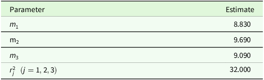
were specified as the mean of reference varieties in a given year (Najewski et al., Reference Najewski, Madajska, Skrzypek and Szarzyńska2023, Reference Najewski, Madajska, Skrzypek and Szarzyńska2024). The means were calculated on three varieties for this reason we set that
 $r_j^2$
(
 $i = 1,2,3$
) were equal 32. The values defining the prior distributions of year means are given in Table 2.
Values defining prior distributions annual means

Further, VCU experts performed REML analyses for the common varieties in each three-year period for the four preceding periods (2016/17–2018/19, 2017/18–2019/20, 2019/20–2020/21 and 2020/21–2022/23). The estimates of variance components were available for these periods (Table S2.1). To obtain reliable scale parameters of variance components, we used the meta-analytic approach proposed by Silva et al. (Reference Silva, Viana, Faria and de Resende2013). However, the variance components do not follow a normal distribution. Studnicki and Piepho (Reference Studnicki and Piepho2024) expressed the variance components on a log scale to construct prior distributions for replicates, blocks and plots based on previous trial results. In the current study, we performed a meta-analysis of the logarithms of standard deviations. Therefore, we reanalysed the previous datasets using the glmmTMB R package (Brooks et al., Reference Brooks, Kristensen, van Benthem, Magnusson, Berg, Nielsen, Skaug, Maechler and Bolker2017). This package provides the standard error for log standard deviations. To combine the information about log standard deviations from the four studies, we used the rma function from the R package ‘metafor’ (Viechtbauer, Reference Viechtbauer2010) for each parameter. To achieve this, we set the options method=‘REML” and weighted=TRUE. To validate the inclusion of these estimates in the fixed-effects meta-analysis, a homogeneity test based on the Cochran’s
 $Q$
statistic (Hedges and Olkin, Reference Hedges and Olkin1985) implemented in the metafor package was used. The underlying null hypothesis assumes that the true treatment effect is the same across studies and variations are simply caused by chance. A detailed description of the meta-analysis can be found in Supplement S2.
The two models were compared using the widely applicable information criterion (WAIC; Watanabe, Reference Watanabe2010). Similar to the Akaike information criterion (AIC) in the frequentist approach, the WAIC criterion is a criterion for model selection based on the idea that smaller is better. The choice of model was based on the difference between the two WAIC values.
Markov chain Monte Carlo methods (Metropolis-within-Gibbs sampling and posterior predictive sampling for missing values) were used to fit all models. For this, we used the R package ‘NIMBLE’ (de Valpine et al., Reference de Valpine, Turek, Paciorek, Anderson-Bergman, Lang and Bodik2017, Reference de Valpine, Paciorek, Turek, Michaud, Anderson-Bergman, Obermeyer, Wehrhahn Cortes, Rodrìguez, Lang and Paganin2022). The R scripts for both models are provided in Supplement S3. For each model, three Markov chains with different initial values were generated. The convergence of the chains was examined in each model by visually inspecting the trace plots and using the Gelman and Rubin (Reference Gelman and Rubin1992) convergence diagnostic (potential scale reduction factor;
 $\hat R$
) (see also Congdon, Reference Congdon2020), which was implemented in the CODA R-package (Plummer et al., Reference Plummer, Best, Cowles and Vines2006). For each model, the length of the Markov chains was chosen so that
 $\hat R$
was less than 1.08 for each parameter. The length of each chain was therefore set to 300,000 iterations, with a burn-in period of 150,000 iterations and a thinning interval of 4. The estimates of the parameters of interest from all three Markov chains were summarised for all models using the summary function from the MCMCvis R package (Youngflesh, Reference Youngflesh2018). For clarity, only the results for the preferred model are reported.
Results
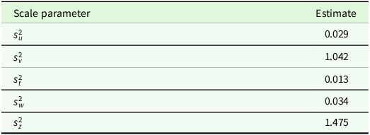
Firstly, we reanalysed the data from previous studies, after which we performed the meta-analysis on the log-standard deviations. The results are presented in Table S2.2 of Supplement S2. Column 6 of Table S2.2 in Supplement S2 reports the combined estimates in log-scale. The Cochran’s Q test was used independently for each variance component. The associated P-values ranged from 0.31 to 0.92, indicating the homogeneity of these independent studies and the adequacy of combining their results into a single measure (see Supplement S2). The values of the scale parameters
 $s_l^2$
(
 $l = u,v,t,w,z$
) are given in Table 3 (see also the final column of Table S2.2).
Estimates of scale parameters
 $s_l^2$
(
 $l = u,v,t,w,z$
)

Next, the scale parameters
 $s_l^2$
(
 $l = u,v,t,w,z$
) were used to fit the models M1 and M2 (see Supplement S3). In both models, we assumed that variance components follow scaled-inverse-
 ${\chi ^2}$
-distribution with scale parameter
 $s_l^2$
(
 $l = u,v,t,w,z$
) and 4 degrees of freedom. Initially, the convergence of each model was checked. In each model, the values of
 $\hat R$
for all parameters in the model were less than or equal to 1.01 (Supplements S4 and S5). The convergence of all parameters in each model was also confirmed by inspecting the trace plots. The Markov chains showed good convergence for each model. Diagnostic plots for the parameters of interest in models M1 and M2 can be found in Supplements S6 and S7, respectively. The WAIC value for model M1 was equal to 1499.68 and was higher than the WAIC value for model M2 (1496.95). This means that there was no substantial gain from introducing variety-specific genotype-by-year and variety-by-location variances. Figure 3 shows the highest posterior intervals for the variance components
 $\sigma _{{t_i}}^2$
and
 $\sigma _{{w_i}}^2$
, in Model M1 (
 $i = 1,2, \ldots, I$
).
Highest posterior density intervals for
 $\sigma _{{t_i}}^2$
(a) and
 $\sigma _{{w_i}}^2$
(b) (
 $i = 1,2, \ldots, I$
).

For all variance components, the highest posterior intervals for
 $\sigma _{{t_i}}^2$
included 0.01 (see Figure 3a). This indicates that there is evidence that all
 $\sigma _{{t_i}}^2$
can be treated as constant. A similar pattern can be observed for variance components
 $\sigma _{{w_i}}^2$
(Figure 3b). For these components, the highest posterior intervals included 0.04. Therefore, following the principle of parsimony, we prefer to choose model M2.
In the subsequent stage of the analysis, the sensitivity of the estimates of variance components to the choice of prior distributions for the variance components in model M2 was investigated. For the purpose of this study, model M2 was fitted with different priors for
 ${\rm{\sigma }}_l^2$
(
 $l = u,v,t,w,z$
) within the family of scaled-inverse-
 ${{\rm{\chi }}^2}$
distributions and for
 ${{\rm{\sigma }}_l}$
within half-t (Ht), uniform (U) and beta (Be) distributions
 $$M2b: {\rm{\sigma }}_l^2 \sim IC\left( {0.2,s_l^2} \right) (l = u,v,t,w,z);$$
 $$M2c: {{\rm{\sigma }}_l} \sim \left( {0,50} \right) (l = u,v,t,w,z);$ $$
 $$M2d: {{\rm{\sigma }}_v} = 50{\rm{B}}{e_1}; {{\rm{\sigma }}_z} = 50{\rm{B}}{{\rm{e}}_2}; {\rm{B}}{{\rm{e}}_{\rm{p}}} \sim B{\rm{e}}\left( {1 + {\rm{\varepsilon }},1 + {\rm{\varepsilon }}} \right), p = 1,2;$$
 $${{\rm{\sigma }}_l} \sim U\left( {0,50} \right) l = u,t,w.$$

The prior distribution in the fourth line can be treated as an alternative to uniform distribution (Figueroa-Zúñiga et al., Reference Figueroa-Zúñiga, Arellano-Valle and Ferrari2013). In the present study, we specified that
 ${\rm{\varepsilon }} = 0.1$
. The results of the sensitivity analysis are summarised in Table 4. The estimates of variance components from model M2 are reported in the first row (M2a).
Posterior estimates of variance components (mean; 95% credible interval, CI) in model M1 with prior distributions to the variance components in model M1

The lowest value of the WAIC criterion was obtained for model M2a. It can also be seen that there are no large differences between the five models. This already indicates a certain robustness in the estimation of the model parameters, regardless of the prior distributions of the variance components. A comparison of the estimates of the variance components reveals that under these divergent priors, analogous posterior estimates of the variance components were obtained. This begins to indicate some robustness of the model to the prior distributions of the variance components. Therefore, the results from model M2a are reported. The analysis of the dataset with model M2a yielded several parameter estimates (Tables 4 and 5).
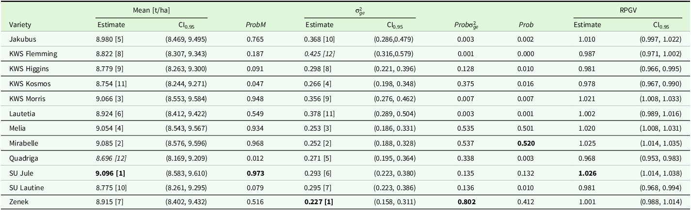
Posterior variety means, probability that the mean yield of a given variety exceeds the general mean, GEI variances (
 ${\rm{\sigma }}_{ge,i}^2$
), probability that the GEI variance would be smaller than the first percentile of the
 $\sigma _{ge,i}^2$
variances, joint probability of superior performance and stability, the relative performance genotypic value index (RPGV)

In the first row of Table 4, the posterior estimates of variance components with their 95% credible intervals (CI0.95) are reported. It can be noticed that the both variance components for year
 $ \times $
site interaction and for sites were almost equal. At the same time, these two effects explained much of the variability in the dataset.
Posterior variety means, probability that the mean yield of a given variety exceeds the general mean, GEI variances (
 ${\rm{\sigma }}_{ge,i}^2$
), probability that the GEI variance would be smaller than the first percentile of the
 $\sigma _{ge,i}^2$
variances, joint probability of superior performance and stability, the relative performance genotypic value index (RPGV) are reported in Table 5. The probability distributions for variety means, for GEI variance and the RPGV indices are shown in Supplement S7
Posterior variety mean yields, 95% credible intervals and probabilities of superior performance are given in the second, third, and fourth columns of Table 5, respectively. It can be noticed that the mean yields ranged from 8.696 t/ha to 9.096 t/ha. The highest yield was recorded for variety SU Jule. Furthermore, it can be noticed that the mean yields for varieties KWS Morris, Melia and Mirabelle exceeded 9 t/ha. On the other hand, based on the ProbM values one can distinguish two separate groups: (i) group of varieties for which probability ProbM was higher than 0.5 and (ii) group of varieties for which probability ProbM was less or equal to 0.5. The first group consisted from varieties: Jakubus, KWS Morris, Lautetia, Melia, Mirabelle, SU Jule, and Zenek. To the latter group included variety KWS Flemming, KWS Higgins, Quadriga and SU Latine. For the varieties in this group, the values of ProbM did not exceed 0.2. This means that farmers are taking a risk when choosing varieties from this group.
Figure 4 shows the pair-wise probabilities of superior performance. For clarity, the varieties have been arranged in descending order in the heatmap.
All pair-wise probabilities for variety means. Varieties were ordered in the descending order. The variety codes are as follows: v1 = Jakobus; v2 = KWS Flemming; v3 = KWS Higgins; v4 = KWS Kosmos; v5 = KWS Morris; v6 = Lautetia; v7 = Melia; v8 = Mirabelle; v9 = Quadriga; v10 = SU Jule; v11 = SU Lautine; v12 = Zenek. The pair-wise probabilities of superior performance (
 $P\left( {M{V_i}\gt M{V_{i'}}{\rm{|}}y} \right)$
) are shown below the diagonal, whereas the values of the probabilities for the opposite events are shown above the diagonal.

It can be seen that the highest values of the pair-wise probabilities of superior performance were found for variety SU Jule. The pair-wise probabilities for this variety varied from 0.538 to 0.998. Moreover, it can be noted that the probability that mean yield for variety Mirabelle would be higher than the mean yield for variety SU Jule was equal to 0.462. For varieties KWS Morris and Melia the pair-wise probabilities were equal 0.396 and 0.359, respectively. On the other hand, the lowest values of the pair-wise probabilities superior performance were obtained for variety Quadriga. The values of the probabilities for this variety did not exceeded 0.3 (see Supplement S5).
Columns five, six and seven of Table 5 show the posterior estimates of the GEI variances, 95% CIs and probabilities
 ${\rm{\;Prob}}{\sigma _{ge,i}}$
. It can be seen that the smallest GEI variance was obtained for variety Zenek. This indicates that this variety was the most stable of those included in the analysis. The second and third best varieties in terms of GEI variance were Mirabelle and Melia, respectively. The variety with the highest yield (SU Jule) was ranked sixth. On the other hand, the variety with the highest GEI variance was KWS Flemming. Furthermore, it can be seen that for the first three most stable varieties the probabilities
 ${\rm{Prob}}{\sigma _{ge,i}}$
were higher than 0.5. In addition, by taking a set of the first three most stable varieties and a set of varieties for which the probability ProbM was greater than 0.5, it can be seen that both sets overlap. Moreover, it can be seen that the set of the three most stable varieties is also the common part of the two sets. This was confirmed by the highest values of the joint probability of superior performance and stability (Prob, eighth column of Table 5).
Figure 5 shows the pair-wise probabilities for the GEI variances. For clarity of presentation, the varieties have been ordered from most stable to least stable.
All pair-wise probabilities for stability variances. Varieties were ordered ascendingly. The variety codes are as follows: v1 = Jakobus; v2 = KWS Flemming; v3 = KWS Higgins; v4 = KWS Kosmos; v5 = KWS Morris; v6 = Lautetia; v7 = Melia; v8 = Mirabelle; v9 = Quadriga; v10 = SU Jule; v11 = SU Lautine;v12 = Zenek. The pair-wise probabilities for GEI variances (
 $P( {{\rm{\sigma }}_{ge,i}^2\gt {\rm{\sigma }}_{ge,i'}^2|y} )$
) are shown below the diagonal, whereas the values of the probabilities for the opposite events are shown above the diagonal.

In general, the lowest values of the pair-wise probabilities for GEI variances were obtained for the Zenek variety. The pair-wise probabilities for this variety varied from 0.003 to 0.285, with the highest values obtained in comparisons with Mirabelle and Melia. On the other hand, the highest values of the pair-wise probabilities for GEI variances were obtained for variety KWS Flemming. The probabilities for this variety exceeded 0.7 (see Figure 5 and Supplement S5).
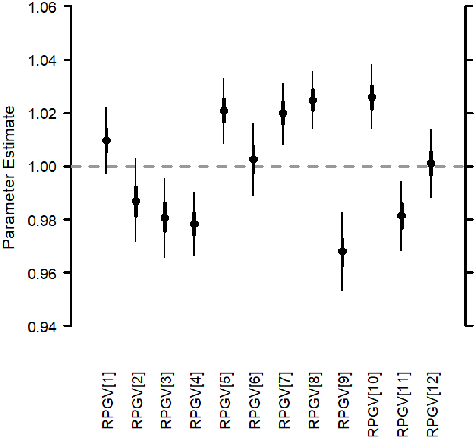
Finally, the predicted variety x environment interaction means were used to calculate the RPGV indices. The values of the RPGV index, along with their 95% confidence intervals (CIs), are provided in the final two columns of Table 5. In Figure 6, the highest posterior density intervals for the values of the RPGV index are plotted.
Highest posterior density intervals for the RPGV indices.

It can be observed that for only four varieties (Jakubus, Lautetia, Quadriga and Zenek) the 95% CI included 1, which means that for these varieties the values of the RPGV index were not significantly different from 1. For the rest of the varieties, the values of the RPGV index were significantly higher or significantly lower than 1. Furthermore, the highest values of the RPGV index were obtained for the varieties SU Jule and Mirabelle. This means that these two varieties showed a high adaptability to the agro-meteorological conditions of the environments. The third highest yielding variety was also the third best in terms of RPGV, while the most stable variety was ranked seventh.
Discussion
Using stable and well-adapted varieties is the most effective and environmentally friendly way to cope with unpredictable stresses caused by climate change. In the literature, stability and adaptability are typically assessed using a combination of Wricke’s ecovalence stability coefficient (Wricke, Reference Wricke1962) and the Finlay–Wilkinson model (FW; Finlay and Wilkinson, Reference Finlay and Wilkinson1963) (Sandro et al., Reference Sandro, Kucek, Sorrels, Dawson and Gutierrez2022), or by fitting the Eberhart-Russell model (ER; Eberhart and Russell, Reference Eberhart and Russell1966), or by using best unbiased linear predictions and restricted maximum likelihood to calculate the harmonic mean of the relative power of genotypic values (HMRPGV; Craine et al., Reference Craine, Choi, Schroeder, Brueggeman, Esser and Murphy2023). All these models can be fitted using either a one- or two-stage approach. In the former approach, plot data from all trials are used to estimate the parameters of interest in a model (e.g. a linear mixed model). In the latter, each trial is first analysed separately, after which the variety means from all trials are analysed using a linear mixed model or the ER model.
In the present work, a two-stage approach was used to analyse the three-way variety
 $ \times $
year
 $ \times $
location data. A similar approach has been considered, for example, by Caliński et al. (Reference Caliński, Czajka and Kaczmarek1987a,Reference Caliński, Czajka and Kaczmarekb), Czajka (Reference Czajka1995), Laidig et al. (Reference Laidig, Drobek and Meyer2008) and Piepho and van Eeuwijk (Reference Piepho, van Eeuwijk and Kang2002). The main reason for this approach was that it better reflects the structure of the data than the two-way data approach used in the literature (see e.g. Craine et al., Reference Craine, Choi, Schroeder, Brueggeman, Esser and Murphy2023; or Sandro et al., Reference Sandro, Kucek, Sorrels, Dawson and Gutierrez2022). Piepho and van Eeuwijk (Reference Piepho, van Eeuwijk and Kang2002) showed that, in reality, observations from the same year at different sites and from the same site but different years are correlated, whereas for the two-way variety
 $ \times $
environment data, observations from all environments are treated as independent. In the same study, they pointed out that it is usually difficult to perform the three-way mixed model analysis for multi-environment trial data due to the small number of years and sites relative to the number of genotypes. Furthermore in this study, a generalised stability variance (Piepho, Reference Piepho1994) was used as a stability measure which is a function variety-by-year variety-specific variances (
 $\sigma _{GY,i}^2$
), variety-by-location variety-specific variances (
 $\sigma _{GL,i}^2$
) and residual variety-specific variances (
 $\sigma _{e,i}^2$
). Piepho (Reference Piepho1994) argued that a reliable assessment of stability, including the genotype × year interaction, requires ten or more years of testing. However, this is not feasible in most VCU trials, since by the time sufficient data have been compiled, the varieties under consideration will likely have been withdrawn from trials or removed from the NL list. Furthermore, some varieties may have zero estimates for the variance components
 $\sigma _{GL,i}^2$
or/and
 $\sigma _{GY,i}^2$
. For this reason, Bayesian hierarchical models were used in the current study. This approach allowed us to use prior knowledge of the annual means. As a prior estimate of the annual mean, we used the mean of the reference varieties in a given year. We increased the uncertainty in the annual means by assuming that the variances were equal to 32. A normal distribution with such variances can be treated as weakly informative (Lemoine, Reference Lemoine2019; Carpenter, Reference Carpenter2023). On the other hand, Banner et al. (Reference Banner, Irvine and Rodhouse2020) and Carpenter (Reference Carpenter2023) did not recommend using vague priors for means and intercepts in regression analysis. As variety offices and breeding companies have long-term data, it is possible to update the hyperparameters, and therefore the knowledge of the variance components (see, e.g., Laidig et al., Reference Laidig, Drobek and Meyer2008). Several methods for constructing informative priors for variance components from a single trial have been proposed in the literature. For example, Silva et al. (Reference Silva, Viana, Faria and de Resende2013) used a meta-analytic approach to construct informative priors by combining ANOVA and REML estimates from previous studies with estimates of variance components from analyses using non-informative priors. In order to verify the incorporation of the aforementioned two studies within their meta-analysis, they applied a homogeneity test based on the Q-test statistic (Hedges and Olkin, Reference Hedges and Olkin1985). In a different study, Singh et al. (Reference Singh, Al-Yassin and Omer2015) constructed informative priors for a set of 20 field trials with similar experimental designs. More recently, Studnicki and Piepho (Reference Studnicki and Piepho2024) used hierarchical models to construct objectively informed prior distributions for the variance components of replicates, blocks and plots based on the results of previous trials. In this study, the number of sites varied from 35 to 43 depending on the growing season. They implemented their models using empirical Bayes and a fully Bayesian approach. In the current study, prior information about the likely values of the variance components
 $\sigma _l^2$
(
 $l = u,v,w,t,z$
) and their standard errors were available from only four previous analyses For this reason, a meta-analytic approach was used to obtain reliable estimates of the scale parameters. However, the variance components do not follow a normal distribution. In the current study, we therefore first reanalysed the data from previous studies before performing the meta-analysis on the log-standard deviations to construct reliable scale parameters for these variance components. As in Silva et al. (Reference Silva, Viana, Faria and de Resende2013), we used a Q-test statistic for each parameter to validate the inclusion of these studies in the meta-analysis. If the analysis of a previous study yields a zero estimate for the variance component, one can refit the dataset using a Bayesian hierarchical model with non-informative priors. Next, replace the variance component estimates for this dataset and perform the meta-analysis. An alternative solution to this problem is to assume a non-informative prior in the Bayesian model for the variance component with a missing value from the previous analysis. When estimates from a larger number of multi-environmental analyses are available, the approach of Singh et al. (Reference Singh, Al-Yassin and Omer2015) or Studnicki and Piepho (Reference Studnicki and Piepho2024) should be preferred. Furthermore, Bayesian analysis enables posterior distributions of new quantities, which are functions of model parameters, to be computed. In this paper, the posterior distributions of the RPGV indices were calculated. Finally, using MCMC samples, we calculated the probabilities of superior performance, the probability that the GEI variance is less than the first percentile of
 $\sigma _{ge,i}^2$
variances, and a joint probabilities of superior performance and stability. A similar approach was used by Dias et al. (Reference Dias, dos Santos, Krause, Piepho, Guimarães, Pastina and Garcia2022), Przystalski and Lenartowicz (Reference Przystalski and Lenartowicz2023) and Chaves et al. (Reference Chaves, Krause, Dias, Garcia and Dias2024). In all these studies, the authors used a Bayesian probabilistic approach to facilitate the decision-making process for variety recommendations. More recently, the probabilistic concepts to support the recommendation of varieties in breeding programmes have been implemented in the ProbBreed package (Chaves et al., Reference Chaves, Krause, Dias, Garcia and Dias2024).
The current study shows that SU Jule and Mirabelle had the highest yields of all the varieties tested, while Quadriga had the lowest. Furthermore, Zenek was the most stable variety, with Mirabelle ranking second. According to the RPGV index, the varieties with the highest yields were also well adapted to the agro-meteorological conditions. The highest
 ${\rm{Prob}} \,\sigma _{ge}^2$
values were obtained for Zenek, Mirabelle and Melia, and the ProbM values for these varieties were all greater than 0.5. Moreover, these three varieties had the highest joint probabilities of superior performance and stability. Therefore, it can be concluded that Melia, Mirabelle and Zenek should be favoured.
Probabilistic methods combined with Bayesian hierarchical models are a powerful tool for selecting the most promising lines or for selecting the best varieties for cultivation. The probability concepts in variety recommendation were first introduced in a frequentist approach by Mead et al. (Reference Mead, Riley, Dear and Singh1986). Eskridge and Mumm (Reference Eskridge and Mumm1992) calculated the probability of dominance of the control for each variety. They then selected the variety with the highest probability of superiority. Piepho (Reference Piepho1996) introduced the concept of relative risk, which can be treated as a counter-example to pair-wise probabilities of superior performance to some extent. Dias et al. (Reference Dias, dos Santos, Krause, Piepho, Guimarães, Pastina and Garcia2022) were the first to consider the probability concepts in variety recommendations using posterior samples from a Bayesian hierarchical model. In the present study, we calculated the probability that the mean of a given variety would exceed the overall mean and the probability that the stability variance of a given variety would be in the first percentile. We supplemented the analyses by calculating the pair-wise probabilities of superior performance and pair-wise probabilities for stability variances. Both Miranda et al. (Reference Miranda, Dias, Júnior, Carneiro, Carneiro, Carneiro, Souza, Melo, Pereira, Vieira and Martins2024) and Chaves et al. (Reference Chaves, Krause, Dias, Garcia and Dias2024) were also interested in selecting the variety that performed best. Miranda et al. (Reference Miranda, Dias, Júnior, Carneiro, Carneiro, Carneiro, Souza, Melo, Pereira, Vieira and Martins2024) conducted their analyses using a two-way variety × environment table, whereas Chaves et al. (Reference Chaves, Krause, Dias, Garcia and Dias2024) analysed two- and three-way datasets. We also calculated the joint probability of superior performance and stability for each variety. In the current study, the joint probabilities for the best-performing varieties were approximately 0.5; in the studies of Dias et al. (Reference Dias, dos Santos, Krause, Piepho, Guimarães, Pastina and Garcia2022) and Chaves et al. (Reference Chaves, Krause, Dias, Garcia and Dias2024), the joint probabilities were approximately 0.3. However, in contrast to Dias et al. (Reference Dias, dos Santos, Krause, Piepho, Guimarães, Pastina and Garcia2022) and Chaves et al. (Reference Chaves, Krause, Dias, Garcia and Dias2024), we calculated the joint probabilities without assuming independence between the two events (see Supplement S3). Dias et al. (Reference Dias, dos Santos, Krause, Piepho, Guimarães, Pastina and Garcia2022) concluded that the independence assumption could be strong. Therefore, they first calculated the Pearson correlation between the variety effects and the stability variances. For this reason, it is recommended to check the correlation between variety effects and stability variance before calculating the joint probabilities using the independence assumption. Further, both Bayesian and frequentist probabilistic methods can be considered as quick and straightforward approaches that facilitate the decision-making process regarding variety recommendations. From a broader perspective, crop variety recommendations can be viewed as an example of decision-making under uncertainty. Such problems are often solved using concepts from the theory of optimal statistical decisions (DeGroot, Reference DeGroot1970). Theobald et al. (Reference Theobald, Roberts, Talbot and Spink2006) and Przystalski and Lenartowicz (Reference Przystalski and Lenartowicz2020) employed Bayesian decision theory to estimate economically optimal seed rates for winter wheat and recommend potato varieties for future sowing, respectively. To achieve this, they first fitted Bayesian hierarchical models and then used utility functions to calculate the posterior expected utility of each variety. In a genetic study, Villar-Hernandez et al. (Reference Villar-Hernández, Pérez-Elizalde, Crossa, Pérez-Rodriguez, Toledo and Burgueño2018, Reference Villar-Hernández, Pérez-Elizalde, Martini, Toledo, Perez-Rodriguez, Krause, Garcia-Calvillo, Covarrubias-Pazaran and Crossa2021) applied a Bayesian framework to genomic selection. They derived and expressed several loss functions in terms of heritability, and tested them on real wheat data for one selection cycle and in a simulated selection programme. They concluded that using a loss function would be a useful criterion for selecting candidates for the next breeding cycle.
All of the models fitted in this study were programmed using the NIMBLE package (de Valpine et al., Reference de Valpine, Turek, Paciorek, Anderson-Bergman, Lang and Bodik2017; Reference de Valpine, Paciorek, Turek, Michaud, Anderson-Bergman, Obermeyer, Wehrhahn Cortes, Rodrìguez, Lang and Paganin2022). The model definition within this package is less formalised than in Stan (Stan Development Team, 2024). Furthermore, the package uses a syntax similar to that of JAGS and WinBUGS, which may appeal to non-statisticians who are familiar with these two packages. The package also allows users to extend the list of implemented distributions and define their own functions and distributions. In the current study, the scaled-inverse-
 ${\chi ^2}$
distribution with small degrees of freedom was used as the prior distribution for the variance components. We preferred this approach because our prior estimates of scale parameters were based only on the results from four studies. Larger degrees of freedom indicate greater confidence in the prior estimate. Furthermore, this approach ensures a finite prior expectation (Pérez et al., Reference Pérez, de los Campos, Crossa and Gianola2010). In this study, we chose an inverse-Gamma distribution from the extended list of available probability distributions in the package to parameterise the distributions for the variance components. To check the robustness of our variance component priors, we complemented our analysis with a sensitivity analysis. Sorensen and Gianola (Reference Sorensen and Gianola2002) argued that this is an important part of Bayesian inference. In their book, they showed how to perform sensitivity analysis using importance sampling. In the current paper, we took a different approach and considered four alternative priors:
 $IC\left( {{s^2},0.2} \right)$
,
 $U\left( {0,50} \right),$
 $50Be\left( {1 + \varepsilon, 1 + \varepsilon } \right)$
, and normality of log-standard deviations. The first was used by Theobald et al. (Reference Theobald, Talbot and Nabugoomu2002) in their study on the application of the Bayesian approach to regional and local area prediction from crop variety trials. The third, according to Figueroa-Zúñiga et al. (Reference Figueroa-Zúñiga, Arellano-Valle and Ferrari2013), can be considered as an alternative to the uniform distribution, which is more flexible. The latter prior distributions are examples of direct application of the results of the estimates of meta-analysis. We assumed that variances were equal to 2 and 1 for
 $l = u,v,w,z$
and
 $l = t$
, respectively, because the meta- analysis estimates were based only on the results from four studies. Under these quite different priors, we obtained similar posterior estimates of the variance components. A similar approach to sensitivity analysis was used by Rodrigues-Motta and Forkman (Reference Rodrigues-Motta and Forkman2022).
Finally, to the best of our knowledge, there is no procedure for constructing reliable prior estimates of variance components for the analysis of multi-environmental trial series. In Poland, 20 to 40 sites are used each year in post-registration trials for major crops. Using the approach proposed by Studnicki and Piepho (Reference Studnicki and Piepho2024), one could construct an objective prior at least for the effects of varieties, sites and variety
 $ \times $
site interaction. From this point of view, it would be worthwhile to compare their method of constructing informative priors for variance components with the meta-analytic approach considered in this study. Furthermore, only normally distributed responses were considered in this study. However, non-normally distributed traits are also observed in VCU and plant breeding trials, such as resistance to European corn borer (Przystalski and Lenartowicz, Reference Przystalski and Lenartowicz2017) or resistance to sclerotinia (Zawieja et al., Reference Zawieja, Slebioda and Mikulski2023). By modifying the described models, it would be possible to identify stable and highly resistant varieties. We plan to investigate this topic in a future study.
Supplementary material
For supplementary material accompanying this paper visit https://doi.org/10.1017/S0021859625100233
Data availability statement
Data were provided by Research Centre for Cultivar Testing Poland for exclusive use in this study and are, in general, not publicly available. Reasonable requests may be addressed to the Research Centre for Cultivar Testing, Słupia Wielka, Poland.
Acknowledgements
We would like to thank the Research Centre for Cultivar Testing (Słupia Wielka, Poland) for providing the data that was used in the present study.
Author contributions
MP perceived the idea of investigating the topic. MP proposed the statistical methodology and performed the statistical analyses. MP wrote the early version of the manuscript and revised it.
Funding statement
This research received no specific grant from any funding agency, commercial or not-for-profit sectors.
Competing interests
The authors declare there are no conflicts of interest.
Ethical standards
Not applicable.