1. Introduction
Hydrodynamic impact problems are commonly encountered in various engineering applications, including the water landings of spacecraft and seaplanes (Seddon & Moatamedi Reference Seddon and Moatamedi2006), bow slamming during the re-entry of a ship into water (Kapsenberg Reference Kapsenberg2011), and wet-deck slamming on vessels and offshore structures (Faltinsen Reference Faltinsen2000; Faltinsen, Landrini & Greco Reference Faltinsen, Landrini and Greco2004). During these events, the structure undergoes a rapid interaction with water, generating significant impact forces within a very short period. Similarly, in competitive diving from a 10 m platform, athletes hit the water at speeds exceeding 14 m s−1, subjecting their bodies to substantial impact forces (Ma et al. Reference Ma, Causon, Qian, Mingham, Mai, Greaves and Raby2016). Prolonged exposure to such high-intensity impacts poses considerable risks to both structural integrity and human health. Therefore, accurate prediction of impact loads is vital for both structural design and human safety in high-impact scenarios.
The earliest research on water entry impact pressures began with von Karman (Reference von Karman1929), who developed a simplified model to predict the impact force on a wedge and flat plate, based on the law of conservation of momentum and added mass system. Wagner (Reference Wagner1932) later expanded this work by accounting for pile-up of the water, deriving a more refined model for a rigid wedge entering water. Wagner’s model, while still based on assumptions of incompressible and potential flow, improved the accuracy of predictions by applying linearised boundary conditions on the initial free surface. After that, many researchers improved Wagner’s theory, further advancing the understanding of water entry impact phenomena, including Zhao & Faltinsen (Reference Zhao and Faltinsen1993), Korobkin (Reference Korobkin2004) and Howison, Ockendon & Wilson (Reference Howison, Ockendon and Wilson1991). On the other hand, numerous experimental studies have been undertaken to investigate water impact loads by dropping a simple-shaped object, such as a flat-bottom plate (Ermanyuk & Ohkusu Reference Ermanyuk and Ohkusu2005), a wedge (Jain et al. Reference Jain, Novaković, Bogaert and van der Meer2022) and a cylinder (Van Nuffel et al. Reference Van Nuffel, Vepa, De Baere, Lava, Kersemans, Degrieck, De Rouck and Van Paepegem2014). Lafeber, Bogaert & Brosset (Reference Lafeber, Bogaert and Brosset2012) introduced the concept of elementary loading process (ELPs) to describe the loading processes based on the experimental results from the Sloshel project. It is assumed that each slamming event can be described as a combination of three ELPs (Dias & Ghidaglia Reference Dias and Ghidaglia2018). Of these, ELP2 is the most common type in engineering applications including water entry impact, characterised by the run-up of liquid along a solid surface. This run-up process induces rapid changes in fluid pressure and velocity, generating significant forces due to the change of fluid momentum. In contrast, ELP1 refers to direct impact scenarios, occurring when a solid stops a fluid or vice versa. Type ELP1 is marked by a sudden, near-discontinuous acceleration or deceleration of the fluid, resulting in pressure waves that travel at the speed of sound through the liquid. Jet impingement on a solid wall or flat plate water entry are included in this category. Type ELP3 occurs when air bubbles or air pockets are entrapped during the impact process. For a water entry problem, it is more likely to occur when the relative angle between the body and the fluid is smaller than 5° (Dias & Ghidaglia Reference Dias and Ghidaglia2018). Several researchers have pointed out that the air entrapment greatly affects the evolution of impact pressures on the solid body, making it difficult to fully understand the underlying physical processes and mechanisms involved in water entry (Huera-Huarte, Jeon & Gharib Reference Huera-Huarte, Jeon and Gharib2011; Van Nuffel Reference Van Nuffel2014). Moreover, in open oceans, bubbles are introduced into the water through various processes, including biological activity, wave breaking, melting snow and white capping (Crawford Reference Crawford1999). These bubbles tend to persist for extended periods in seawater, remain small, and rise slowly due to their resistance to coalescence. The water entry impact problem becomes increasingly complex due to the presence of pre-existing bubbles in the water (i.e. aerated water).
There has been limited research on the impact loads of water entry in aerated conditions, despite its practical importance. Ma et al. (Reference Ma, Causon, Qian, Mingham, Gu and Ferrer2014) examined the effects of air entrapment and aeration on wave impact through numerical simulations, treating the flow as a compressible air–water mixture governed by conservation laws and gas phase volume fraction dynamics. Later, Ma et al. (Reference Ma, Causon, Qian, Mingham, Mai, Greaves and Raby2016) implemented numerical simulations based on the compressible multiphase flow model to investigate the water entry of a rigid square flat plate into pure and aerated water. Aghaei et al. (Reference Aghaei, Schimmels, Schlurmann and Hildebrandt2020) completed an extensive numerical investigation into the effects of aeration and hydroelasticity on slamming loads, and the structural behaviour of elastic plates during water entry, under the assumption of isothermal conditions. These studies consistently pointed out that introducing aeration can significantly reduce both local pressures and overall impact forces. Nevertheless, the current numerical simulations remain inadequate to meet the demands of industrial and academic research, primarily due to the extreme complexity of the phenomena involved. Meanwhile, deriving theoretical models for aerated water entry impact is challenging due to the complex gas–liquid interactions, nonlinearity, and the difficulty in accurately modelling the behaviour of air bubbles and fluid compressibility during high-speed impacts. Consequently, laboratory experiments are essential for investigating the impact load in aerated water entry.
Early impact experiments on aerated water were reported by Eroshin et al. (Reference Eroshin1980), who examined the effects of bubbly water on disks to establish correlations between maximum impact forces and void fraction. Walkden (Reference Walkden1999), followed by Bullock et al. (Reference Bullock, Crawford, Hewson, Walkden and Bird2001), conducted drop tests on flat plates for quantifying the effects of aeration on wave impacts. In these studies, the maximum impact force or pressure was noted to decrease with increasing void fraction, particularly at higher impact velocities. More recent experiments by Ma et al. (Reference Ma, Causon, Qian, Mingham, Mai, Greaves and Raby2016) and Mai et al. (Reference Mai, Mai, Raby and Greaves2019) investigated the water entry of rigid square flat plates into both pure and aerated water. Elhimer et al. (Reference Elhimer, Jacques, El Malki Alaoui and Gabillet2017, Reference Elhimer, El Malki Alaoui, Gabillet and Jacques2022) investigated the water entry of cones into aerated water, demonstrating a significant reduction in impact loads due to aeration, even at void fractions below 1 %. Hong, Wang & Liu (Reference Hong, Wang and Liu2021) carried out both experimental and numerical studies on disk impacts into pure and aerated water, revealing that higher aeration levels lead to a more uniform pressure distribution and a 33 % reduction in peak pressure. Chuang (Reference Chuang2022) focused on flat plate impacts, and illustrated that the aeration not only reduces peak pressures but also causes irregular jet flows, further correlating local void fractions with impact pressures. Most of the studies in the existing literature concentrated on the impact of flat-bottomed structures, and therefore pertain to ELP1 since these do not represent water entry scenarios technically (Elhimer et al. Reference Elhimer, El Malki Alaoui, Gabillet and Jacques2022). Furthermore, the classic problem of wedge water entry under aerated conditions has been studied rarely. To date, no comprehensive quantitative experimental studies have been reported on the impact loads experienced by wedges entering aerated water.
Accurate measurement of void fraction is crucial in understanding the impact of aeration on water entry dynamics, as several studies have shown an inverse relationship between aeration level and peak pressure or force. Over the past few decades, a variety of techniques have been developed to measure void fraction in two-phase flows. Depending on the required spatial resolution, these measurements can be taken at specific points, along lines, across surfaces, or within volumes. Ma et al. (Reference Ma, Causon, Qian, Mingham, Mai, Greaves and Raby2016) adopted the volumetric method to estimate the global void fraction by measuring the air flow rate and applying an estimation formula. However, this approach requires assumptions regarding bubble velocity and the adiabatic process, which can skew the results. Elhimer et al. (Reference Elhimer, Jacques, El Malki Alaoui and Gabillet2017, Reference Elhimer, El Malki Alaoui, Gabillet and Jacques2022) and Hong, Wang & Liu (Reference Hong, Wang and Liu2021) relied on a single optical probe system for measuring the global void fraction. Chuang (Reference Chuang2022) employed the fibre optic reflectometer technique to measure local void fractions. However, since the probe captures data from only a single point, it may not accurately reflect the void fraction throughout the entire flow field. In contrast, the wire-mesh sensor (WMS), a new flow imaging technology based on the electrical signal, offers high spatial and temporal resolution for capturing flow characteristics across the entire multiphase region (Prasser, Böttger & Zschau Reference Prasser, Böttger and Zschau1998). Currently, the WMS is employed primarily in two-phase flow studies within pipes and rod bundles (Ylönen, Bissels & Prasser Reference Ylönen, Bissels and Prasser2011; Yang & Xiong Reference Yang and Xiong2023). Given the similarities between multiphase flows and bubbly flows, it is anticipated that the WMS could be adapted effectively to determine void fraction in water entry problems.
This paper aims to explore the effects of aeration on the impact pressure during the water entry of a symmetrical wedge. The research employed a custom-designed bubble generator to create controlled aeration levels in the water tank, allowing for systematic experimentation. Additionally, this study marked the first application of the WMS technology in water entry impact research, providing high spatial and temporal resolution to measure void fractions in multiphase flows accurately. The experiments were carried out using a wedge model with deadrise angle 20°, ensuring minimal air cushioning effects during entry. A series of tests was performed at fixed drop height 750 mm and various gas flow rates, systematically altering the void fraction to assess its influence on impact pressures. Furthermore, this study evaluated the influence of aeration on the splash and jet formation during wedge water entry by visualising flow evolution with different levels of aeration. Comparative analyses between pure and aerated water were completed to assess how void fractions affect pressure distribution, splash dynamics, and overall fluid behaviour. Finally, this study offered a quantitative analysis of the relationship between void fraction and normalised peak impact pressures, incorporating both experimental data and probability distribution. The results provide new insights into the role of aeration in mitigating slamming loads, and suggest potential applications for the improved design of marine structures.
2. Experimental set-up and techniques
2.1. Model description
A series of water entry tests was carried out in the State Key Laboratory of Ocean Engineering of Shanghai Jiao Tong University. As illustrated in figure 1, two high-strength supporting steel frames were placed on either side of the water tank. The tank measures 1.5 m in length, 1.25 m in width, and 1.2 m in depth, with the water depth fixed at 0.8 m during the experiments. The wedge-shaped body has length 0.50 m, width 0.25 m, and deadrise angle 20°. The wedge was positioned to fall at the centre of the water tank. To ensure the vertical drop of the wedge, two guide rails were employed, along which the wedge moved via attached sliding blocks. The total weight of the impacting structure, including the wedge model and additional support components, was 23.3 kg. Given the sudden impact forces generated during the water entry of the wedge, two gas springs mounted on the transverse beam were utilised to absorb the shock. The safety ropes were attached between the gas springs and the wedge to decelerate the wedge after impact, preventing it from hitting the bottom wall of the tank. Additionally, a bubble generator was installed at the bottom of the water tank to produce controlled bubble fields.
Sketch of the experimental set-up. Two high-strength supporting steel frames are placed on both sides of a water tank, with dimensions 1.5 m length, 1.25 m width and 1.2 m depth. The water depth was fixed at 0.8 m during the experiments. Two guide rails were employed to ensure a vertical drop. Gas springs and safety ropes are used to absorb impact forces and decelerate the wedge. A bubble generator at the tank’s bottom creates controlled aeration during the tests.

2.2. Instrumentation
The wedge instantaneous position was measured by a laser displacement sensor (Y1TA100QXVT80, wenglor). The sensor was calibrated to range 0–2 m, and the estimated uncertainty on displacement measurement is
 $\pm 1\text{ mm}$
. An additional frame was employed to mount the laser displacement sensor, ensuring that it remained entirely isolated from the drop device. The zero point of the laser displacement sensor was calibrated at the moment when the wedge apex first touched the water surface. The evolution of the wedge velocity was calculated by a numerical differentiation of the displacement signal (Yettou, Desrochers & Champoux Reference Yettou, Desrochers and Champoux2006).
To record the impact sequence, a high-speed camera (HSC, FASTCAM SA-Z, PHOTRON) at 1000 frames per second and
 $1024\times1024$
pixels was used. The instantaneous pressures on the bottom surface of the wedge were measured by 24 strain-gauge-based pressure sensors (PGMC-A-200KPZ15, KYOWA) with 8 mm head diameter and measurement range up to 200 kPa. The pressure sensor surface was designed to be flush with the wedge model surface, minimising any potential disturbances to the flow field. Specific locations as well as the identification numbers of the pressure sensors are detailed in figure 2. Sensors P01 to P06 were positioned along the centreline of one side of the wedge, spaced 20 mm apart. Similarly, sensors P07 to P12 were evenly distributed along the edge of the same side of the wedge, maintaining the same 20 mm spacing between adjacent sensors. The P24 and P03 sensors were installed in the same longitudinal and vertical positions on opposite sides of the wedge, to facilitate symmetry validation. Additionally, sensors P13 to P23 were placed at the same vertical positions but in varied longitudinal positions along the wedge. The impact pressure was acquired by an acquisition system (EDX-5000A, KYOWA) at sampling rate 20 kHz.
Pressure sensor locations and identification numbers (distances in mm). (a) Bottom view, showing the arrangement of 24 strain-gauge-based pressure sensors along the wedge surface. The sensors are labelled P01 to P24, with specific spacing between them. (b) Front view, illustrating the wedge with sensors positioned at varying longitudinal and vertical positions to capture the impact pressure distribution. (c) The physical model, highlighting the sensor installation on the wedge. The sensor surface is flush with the wedge to minimise flow disturbance.

2.3. Aeration techniques
This study aims to quantitatively investigate the influence of void fraction on the pressure subjected by wedge during aerated water entry. To achieve this, a wedge with 20° deadrise angle was selected, as it minimises the formation of air cushion during the water entry process (Huera-Huarte, Jeon & Chuang Reference Chuang1969; Gharib Reference Huera-Huarte, Jeon and Gharib2011; Barjasteh, Zeraatgar & Javaherian Reference Barjasteh, Zeraatgar and Javaherian2016; Park et al. Reference Park, Choi, Lee and Rhee2020), thereby eliminating any confounding effects of air cushioning on the quantification of void fraction. Furthermore, a bubble generator was carefully designed to produce bubbles accurately and controllably, ensuring precise experimental conditions.
2.3.1. Bubble generation
The bubble generator utilised in the aerated impact tests consisted of 48 quartz sand-based porous boxes arranged in two rows, positioned at the exact centre of the tank bottom, as depicted in figure 3. Each quartz sand-based porous box, measuring 300 mm long by 34 mm wide, had a quartz-cast top, and was connected to an air hose at one end. The compressed air, supplied by an air compressor, was regulated through a flow control system before being delivered to the 48 porous boxes via air hoses. The air then escapes into the water through tiny gaps in the quartz, generating bubbles. The flux of the compressed air was monitored using a digital mass flow controller (AS200, Aosong). The flow controlling range is 0–300 l min−1, and the uncertainly on mass flow rate is estimated at ± 0.6l min−1. The air pressure injected into the water was controlled by a pressure regulator and set at 0.4 MPa during the aerated water tests. Accordingly, the aeration level can be adjusted by regulating the gas flow rate.
Picture of the bubble generator: an array of quartz sand-based porous boxes at the bottom of the water tank. The generator consists of 48 quartz sand-based porous boxes arranged in two rows at the centre of the water tank. Each box, measuring 300 mm in length and 34 mm in width, is connected to an air hose at one end.

2.3.2. Void fraction measuring methods
In order to characterise the property of the air bubble field, void fraction measurements in the impact area were carried out using a carefully designed conductance WMS, prior to the water entry tests. The WMS, pioneered by Prasser, Böttger & Zschau (Reference Prasser, Böttger and Zschau1998), has been employed successfully in various two-phase flow fields, including the identification of flow pattern in pipelines. A detailed explanation of the WMS principle is provided in Appendix A to facilitate a thorough understanding of its application.
In this study, the purpose-designed conductance WMS consisted of 64 electrodes per plane, with pitch 4 mm, resulting in
 $64\times64$
crossing points (i.e. a total of 4096 measuring points) uniformly distributed throughout the target region. The effective measuring area of the WMS was
 $256\text{ mm}\times256\text{ mm}$
, which exceeded the measuring area of the pressure sensors (less than
 $250\text{ mm}\times250\text{ mm}$
). The electrodes were made of stainless steel wires with diameter
 $d_{wire}=0.3$
mm, fixed on an acrylic frame of thickness 4 cm. The axial distance between the wire planes was 2 mm. The electrodes were divided into four groups, each comprising 16 electrodes. Each group was connected to the data recording system (WMS200, HZDR) via a standard DB25 interface unit. During the experiment, the WMS was immersed and positioned approximately 0.75 m above the bottom of the tank (figure 4). The effective measurement area of the WMS was aligned with the measurement area of the pressure sensors. Data acquisition was performed at frequency 2500 Hz, with each recording lasting 20 s. The recording process was repeated 10 times for each specific air flow rate.
Photograph of the WMS employed in the tank. The sensor consists of 64 electrodes per plane with a 4 mm pitch. The electrodes, made of 0.3 mm diameter stainless steel wires, are mounted on a 4 cm thick acrylic frame. The WMS, positioned 0.75 m above the tank bottom, covers a measurement area
 $256\text{ mm}\times256\text{ mm}$
. Data were acquired at 2500 Hz for 20 s intervals, repeated 10 times for each air flow rate.

The WMS is a direct technique for detecting multiphase fluid electrical conductivity properties, but the accuracy in measuring void fraction can be influenced by the intrusive effect of the sensor. To validate the WMS measurements, an image-based void fraction measuring (IBVFM) method was employed to evaluate the void fraction. In this experiment, high-speed camera recordings (FASTCAM SA-Z, PHOTRON, with full resolution
 $1024 \times 1024$
pixels at 1000 frames per second) were used to determine the bubble velocities. The processing steps of the captured image sequence are illustrated in figure 5. The bubble field within the tank was visualised from the front using an intense LED array backlighting, creating a strong contrast between the bright bubble edges and the dark background (figure 5a). The phase boundaries were then accurately identified, and the bubbles were labelled (figure 5b) using the image analysis software TEMA Pro (Image Systems Group, Sweden). The same process was repeated for the image captured after a few frames. By applying cross-correlation techniques to consecutive images, the movement of the interfaces over a fixed time interval could be tracked, allowing for the calculation of the average bubble velocity in the
 $z$
-direction,
 $\overline{V_{z}}$
. The void fraction
 $\alpha _{HSC}$
using the optical method can then be calculated as
 \begin{equation} \begin{array}{c} \alpha _{HSC}=\dfrac{Q}{\overline{V_{z}}S},\end{array} \end{equation}
where
 $Q$
denotes the gas flow rate, and
 $S$
is the bubble generation area, approximated by the area of the bubble generator. A detailed comparison of the void fractions obtained by the optical method and the WMS method will be provided in the subsequent sections.
Bubble recognition process using the visualised images for evaluating bubble velocity. Processed image with bubbles identified and labelled, excluding bubbles in the free surface in the calculation.

2.4. Test conditions
The primary parameter of interest is the void fraction of the aerated water. Seven different gas flow rates,
 $Q=0,60,80,100,120,140,180\ \mathrm{l}\ \rm min^{-1}$
, were applied during wedge water entry experiments at a fixed drop height of 750 mm (corresponding to the impact velocity
 $v_{i}=3.2\ \mathrm{m}\ \mathrm{s}^{-1}$
) to determine the impact of void fraction on impact pressures. The origin of the coordinate system is defined as
 $(X,Y)=(0,0)$
at the bottom centre of the wedge, as illustrated in figure 2. The positive
 $X$
-axis extends to the right of the field of view, with the still-water level designated as
 $Z=0$
. Consequently, the initial position of the wedge tip is at
 $Z=750\ \mathrm{mm}$
.
After the bubbles were sufficiently dispersed in the water (at least 15 s of aeration), the wedge drop experiments and data collection were initiated. According to Stokes’ theory (Detsch & Harris Reference Detsch and Harris1989; Liger-Belair et al. Reference Liger-Belair, Marchal, Robillard, Dambrouck, Maujean, Vignes-Adler and Jeandet2000), a bubble with diameter 0.05 mm at water depth 1 m requires approximately 12.26 min to rise to the surface and degas. Additionally, the bubble rise velocity is proportional to the bubble radius. Consequently, after each test, all bubbles with diameters greater than 0.05 mm would have ascended to the water surface, allowing for complete degassing during the inter-test interval of more than 15 min. To ensure the reliability and reproducibility of the data, each experiment was conducted a minimum of five times for a given void fraction.
3. Data processing and analysis
3.1. Void fraction derivation and results
The void fraction, which quantifies the proportion of gas in the two-phase flow, was derived from the conductance data obtained by the WMS. A linear conversion relationship was employed to transform the conductance data into void fraction values, accompanied by a noise filtering process to improve data accuracy. Several key averaged void fractions are defined to characterise the two-phase flow:
-
(i) time-averaged void fraction
 $\overline{\alpha }_{i,j}$
, averaged over all time frames for a specific spatial location
$(i, j)$
-
(ii) spatially averaged void fraction
$\alpha _{k}$
, averaged across all spatial grid locations for a specific time frame
$k$
-
(iii) space–time averaged void fraction
$\alpha$
, a comprehensive measure of the void fraction, averaged over both space and time.


The detailed derivation of these parameters, including the associated equations and noise filtering process, is provided in Appendix A for readers seeking a more comprehensive understanding.
The comparison between the void fractions measured by the WMS method and the IBVFM method is shown in figure 6. Both methods present the mean values along with their respective error bars: the WMS utilises standard deviation (STD), while the IBVFM method displays the range between the minimum and maximum values. The WMS method exhibits smaller errors, which are well within the expected range of the experimental conditions and can be attributed to inherent variations in bubble size and distribution within the aerated water. This implies that the void fraction remains fairly stable over time and space, thereby demonstrating the consistency and reliability of the WMS in capturing the real-time characteristics of the two-phase flow. Although the IBVFM method exhibits a wider error range due to the normal distribution of bubble velocity, calculating the average void fraction based on the mean velocity remains a reasonable approach. The maximum discrepancy in the mean void fraction between the two methods is less than 6.5 %, indicating good agreement. As seen in figure 6, the void fraction determined by the WMS method displays a distinct linear correlation with the gas flow rate (
 $Q$
), aligning with theoretical expectations. The subsequent analysis will be based on the void fraction data obtained from the WMS method, given its demonstrated precision and strong agreement with the alternative measuring technique.
Comparison of void fractions between the WMS and IBVFM methods. The maximum discrepancy in the mean void fraction between the two methods is less than 6.5 %, indicating good agreement.

3.2. Water entry impact pressure
To ensure accurate analysis of the impact pressure data, a wavelet denoising method was applied to remove high-frequency noise from the raw measurements, resulting in the filtering displayed in figure 7. The db4 wavelet was chosen with 8 decomposition levels, following the universal threshold selection rule as described in Wu et al. (Reference Wu, Liu, Xiao, Shan, Kou, Li and Guo2024). This method effectively removed high-frequency noise while preserving the critical features of the pressure impact. All experimental impact measurements were successfully denoised using this approach.
Comparison between the raw and filtered pressure measurements. The raw pressure data are processed using a wavelet denoising method with the db4 wavelet and 8 decomposition levels to remove high-frequency noise.

Symmetry verification was carried out to prove the accuracy of the experimental set-up and measuring equipment. Pressure sensors P03 and P24 were strategically installed on opposite sides of the wedge at symmetrical longitudinal and vertical positions (see figure 2). The impact pressure measurements recorded by both sensors, shown in figure 8, exhibit remarkable consistency between the two data sets. The near-identical pressure profiles between P03 and P24 confirm that the wedge entered the water in a perfectly vertical and symmetrical manner, limiting any potential effects of asymmetry on the results. This symmetry verification reinforces the precision of the experimental set-up, ensuring the reliability of the water entry impact data.
Symmetric verification for impact pressures measured at sensors P03 and P24. The sensors were installed at symmetrical longitudinal and vertical positions on opposite sides of the wedge, as shown in figure 2. The near-identical pressure profiles recorded by P03 and P24 demonstrate the accuracy of the experimental set-up, confirming that the wedge entered the water vertically and symmetrically.

3.3. Repeatability of impact velocity
Since the impact load is closely related to the velocity at which the wedge enters the water, it is essential to assess the repeatability of the impact velocity that was derived from the displacement data captured by a laser displacement sensor. Figure 9 plots the results of five repeated tests, demonstrating an excellent overlap of the displacement curves. The point where
 $S=0$
corresponds to the moment of initial contact between the wedge tip and the water surface. The wedge was released from an initial height
 $H=750$
mm. The close alignment of these curves indicates the satisfied repeatability of the impact velocity, thereby reinforcing the robustness of the experimental data.
Comparison of the descending displacements in five repeat tests. The displacement curves from all five tests show excellent agreement, with the
 $S=0$
point marking the initial contact between the wedge tip and the water surface. The wedge was released from height 750 mm.

4. Results and discussion
4.1. Flow evolution of the wedge water entry
The visualisation of the wedge water entry process at different void fractions is crucial for evaluating the associated impact dynamics and splash characteristics. Figure 10 presents the time evolution of the flow pattern at five selected moments for three different aeration conditions: pure water (
 $\alpha =0$
), a low void fraction (
 $\alpha =0.80\, \%$
), and a higher void fraction (
 $\alpha =1.77\, \%$
). Several repeated tests confirmed the reproducibility of the phenomena hereafter discussed. At all void fraction levels, the initial impact at
 $t=0\ {\mathrm{ms}}$
was characterised by the wedge barely impacting the water surface. At this stage, no significant differences were detected, as expected, in the water’s response at different void fractions, except for the slight disturbances introduced by aeration.
Flow pattern development following wedge impact on water surface with varied void fractions. Top row,
 $\alpha =0.00\, \%$
; middle row,
 $\alpha =0.80\, \%$
; bottom row,
 $\alpha =1.77\, \%$
. All images share the same scale, as indicated by the scale bars.

The most apparent effect of increased aeration can be identified in the development of the water jets and splash dynamics. As the wedge descended further into the water, distinct jets formed. At
 $t=10\ \mathrm{ms}$
, the wedge in pure water (
 $\alpha =0$
) pushed the water aside symmetrically, emerging as neat and coherent jets. Conversely, in the aerated cases (especially at
 $\alpha =1.77\, \%$
), the jets began to show signs of instability, suggesting that the air bubbles present in the water affected the direction and coherence of the jets. As the wedge penetrated deeper into the water (
 $t=30\ \mathrm{ms}$
), the effects of aeration became more pronounced. In pure water, the jets remained symmetrical and continued to move upwards, forming a well-structured splash curtain. However, the aerated cases exhibited significant irregularities. For
 $\alpha =0.80\, \%$
, some structure of splash was retained, but distortions were visible due to the presence of air bubbles. At
 $\alpha =1.77\, \%$
, the jets appeared chaotic, with asymmetrical splashes and noticeable turbulence at the water surface. This chaotic behaviour highlighted the profound influence of void fractions on water entry dynamics.
As the jets progressed to
 $t=60\ \mathrm{ms}$
, the differences became even more striking. In pure water, the splashes induced by jets began to close smoothly, driven by two forces: the surface tension and air pressure drop (Worthington Reference Worthington1908). A distinct shockwave was also generated, accompanied by a strong burst of acoustic noise. However, this phenomenon was not recorded in detail as it was not the primary focus of the present study. Higher void fractions caused more erratic splash behaviour. In the aerated cases, the splash became fragmented and turbulent. Moreover, the air bubbles surrounding the wedge were compressed during the impact, which was visually evident from the increased brightness in the images around the wedge at
 $t=60\ \mathrm{ms}$
. It was inferred that the reduction in impact pressure may be related to the compressibility of the air bubbles in the aerated water.
Finally, at
 $t=120\ \mathrm{ms}$
, the differences were fully developed. The wedge entry for pure water generated a highly symmetrical splash curtain with well-defined, smooth boundaries. As the void fraction increased to
 $\alpha =0.80\mathrm{\, \% }$
, the splash shape became noticeably altered. The splash boundaries became less uniform, with small disruptions in the symmetry. While the splash still retained a somewhat structured appearance, there was a clear impact of the air content in altering water flow dynamics. In the most aerated case,
 $\alpha =1.77\mathrm{\, \% }$
, the wedge’s impact led to significant changes in flow behaviour. The fragmented droplets radiated upwards and outwards in an arc, forming a more chaotic splash that resembled a crown adorned with randomly distributed pearls. A potential explanation for the variation in splash patterns in aerated water was the surface current induced by the bubbles. The surface current caused by the bubbles, moving from the centre towards the sidewalls of the tank, imparted horizontal momentum to the jets in the aerated cases. This resulted in outward-directed jets in aerated water, compared to the more upward and centralised jets in pure water. The fact that the arc of the splash generated at
 $\alpha =1.77\mathrm{\, \% }$
was larger than that at
 $\alpha =0.80\, \mathrm{\% }$
further supported this observation. A similar phenomenon was documented in the experiments conducted by Kimmoun, Ratouis & Brosset (Reference Kimmoun, Ratouis and Brosset2012) and Mai et al. (Reference Mai, Mai, Raby and Greaves2019), where the bubbles generated a surface current that resulted in a delay of the waves within the tank. This surface current imparts horizontal momentum, which can influence the splash dynamics and even the impact pressure distribution. To further explain the effect of the surface current on pressure, it is essential to consider the liquid velocity induced by the bubbles. The induced velocity can be estimated using a three-phase flow model (Kowe et al. Reference Kowe, Hunt, Hunt, Couet and Bradbury1988). In this model, the induced water velocity
 $V_{l}$
can be expressed as
 \begin{equation} \begin{array}{c} V_{l}=\dfrac{\left(1-\alpha _{0}-C_{m}\alpha _{0}\right)V_{l}^{0}+C_{m}\alpha _{0}V_{b}}{1-\alpha _{0}},\end{array} \end{equation}
where
 $\alpha _{0}$
is the void fraction of the gas–liquid mixture, the added mass coefficient of the bubbles
 $C_{m}$
is typically taken as 0.5,
 $V_{l}^{0}$
is the unperturbed fluid velocity far from the bubbles (taken as 0 in this case) and the terminal rise velocity of the bubbles
 $V_{b}$
is 0.3 m s−1. The maximum induced water velocity is calculated to be
 $V_{l}=0.0027\ \mathrm{m}\ \mathrm{s}^{-1}$
. This induced velocity is extremely small compared to the liquid expansion velocity
 $v_{e}$
caused by the impact, which is calculated using Wagner’s theory:
 \begin{equation} \begin{array}{c} v_{e}=\dfrac{{\unicode{x03C0}} v_{i}}{2\tan \beta }=13.8\ \mathrm{m}\ \mathrm{s}^{-1},\end{array} \end{equation}
where
 $v_{i}$
denotes the impact velocity of wedge. Therefore, it is expected that the surface current induced by the bubbles will have minimal impact on the impact pressures. Unfortunately, due to the limitations of the current image data, it remained challenging to quantitatively explain the fluid–structure interaction mechanism during the wedge water entry. Key obstacles included the interference from air bubbles and the necessity for ultra-high frame rate imaging. The flow patterns identified in both aerated cases (
 $\alpha =0.80\, \%$
and
 $\alpha =1.77\, \%$
) shared similarities to some extent, but neither was entirely axisymmetric. This lack of symmetry was linked to the uneven distribution of bubbles in the water, which prevented the development of a perfectly symmetrical flow field.
4.2. Temporal impact pressure distribution
Figures 11 and 12 illustrate the temporal profiles of measured pressures (five repeated measurements) and the averaged pressure at the measuring point (P01) for pure and aerated water environments, respectively. To ensure consistency and avoid underestimating the mean pressure magnitude, the time corresponding to the first peak of the impact pressure was designated as
 $t=0$
, and all data curves were aligned accordingly before averaging. The pressure time series show a satisfactory level of repeatability in the evolution of local hydrodynamic loads. The repeatability is slightly higher in pure water than in aerated water, owing to the absence of bubble-induced disturbances. Consequently, the mean pressure time series can provide a representative depiction of the pressure evolution and its associated features in subsequent analysis.
Time histories of measured pressure (five repeats) and average pressure at P01 for pure water (the dashed orange line denotes zero pressure). Sensor P01 was positioned along the centreline of one side of the wedge, closest to the keel of the wedge, as indicated in figure 2. Each repetition has been filtered using the wavelet denoising method, as described in § 3.2. All repetitions were aligned by setting the time of the first peak of the impact pressure as
 $t=0$
, ensuring consistency before averaging the curves. The same processing was applied to all data in figure 12.

Temporal profiles of measured pressure (five repeats, filtered) and average pressure at P01 for aerated water (the dashed orange line denotes zero pressure). Sensor P01 was placed along the centreline on one side of the wedge, near the wedge’s keel, as shown in figure 2. As in earlier plots, all repetitions were aligned by setting the time of the first peak of the impact pressure as
 $t=0$
, ensuring consistency before averaging the curves.

As shown in figure 11, the pressure profile for the wedge entering pure water was characterised by a sharp peak followed by a rapid decay, with duration approximately 10 ms. The pressur–time histories revealed virtually no oscillations, suggesting that no air cushions were generated during the impact process. The absence of such air layers was crucial for accurately quantifying the effects of aeration on impact pressure, as it ensured that variations in void fraction were solely attributable to the artificially introduced bubbles.
As depicted in figures 12 and 13(b), different from the situation in pure water, the pressure oscillations were more obvious in aerated tests. For the lowest void fraction (
 $\alpha =0.80\, \%$
), the pressure oscillations were moderate, but as the void fraction rose to
 $\alpha =1.77\, \%$
, these fluctuations became more pronounced. From the time histories of P07 and P08 in figure 13(b), the period of the pressure oscillations can be estimated to a few tenths of a millisecond (order
 $10^{-4}\, \mathrm{s}$
). One possible explanation for the oscillations is the pulsation of the bubbles in aerated water. The natural pulsation frequency
 $f_{n}$
(also referred as the Minnaert frequency) of a spherical gas bubble was derived by linearising the Rayleigh–Plesset equation (Brennen Reference Brennen2005) around the equilibrium radius
 $R_{0}$
:
 \begin{equation} \begin{array}{c} f_{n}=\dfrac{1}{2{\unicode{x03C0}} }\sqrt{\dfrac{3KP_{g0}}{\rho _{{w}}R_{0}^{2}}},\end{array} \end{equation}
where
 $K$
denotes the polytropic index of the gas (
 $K=1.4$
for an adiabatic process in air),
 $P_{g0}$
is the equilibrium gas pressure inside the bubble and
 $\rho _{{w}}$
is the water density. In the experiment,
 $P_{g0}$
was of the order of
 $10^{5}$
Pa, and the equilibrium radius of bubbles generated in aerated water was approximately of the order of
 $10^{-3}$
m. Based on these values, the natural bubble frequency was calculated to be
 $3.3\times 10^{3}$
Hz, which aligned with the pressure oscillation periods identified in figure 13. Additionally, a careful examination of the averaged pressure time history in figure 12 reveals that the oscillations were averaged out to some extent. This could be due to phase variations in bubble pulsation across different repeated experiments. Another potential explanation is that the oscillations were caused by random effects, such as oscillating bubbles near the wedge, which would result in the oscillations being averaged out.
Pressure signals from sensors P07 to P12 in a single experiment for pure and aerated water. Sensors P07 to P12 were evenly distributed along the edge of the same side of the wedge as P01 to P06, maintaining 20 mm spacing between adjacent sensors, shown in figure 2.

The wedge also experienced a significant impulse upon impacting the aerated water, but the impact strength was noticeably weaker in comparison to that in pure water. The intensity of the impact load decreased as the level of aeration increased. Additionally, close inspection of figures 13(a) and 13(b) reveals that the duration of the impact event was extended in aerated conditions. These effects could be explained by the cushioning effect of the entrained air, which acted as a buffer between the wedge and the water surface.
Figure 14 depicts the pressure time histories obtained by sensors P01–P06 (centreline of one side of the wedge) and P13–P23 (varied longitudinal positions along the wedge) for the pure water case. In the subsequent analysis, the phase of all pressure data was correctly adjusted to align the start time
 $t_{s}\hspace{0pt}$
of the pressure peak at the P01 sensor with time
 $t=0$
. A threshold value for defining
 $t_{s}$
was adopted as 1 % of the first pressure peak to diminish the effect of data oscillation. It is clearly shown that the impact pressure can be divided into three different stages, characterised by a distinct set of attributes. During the first stage, the contact line reached the height of the sensor resulting in a rapid increase in pressure, which subsequently reached its maximum value. Then the pressure declined gradually as the contact line moved away from the sensor. It can be observed that the peaks in the pressure time history curves for P13–P23 are well aligned, with the maximum time difference among peak moments being only 0.15 ms, corresponding to three sampling data points at sampling frequency 20 kHz. The slight phase difference is likely attributed to non-ideal stillness of the water surface, model fabrication tolerances and sensor installation errors.
Typical time histories of impact pressures in pure water. Sensors P01–P06 were positioned along the centreline of one side of the wedge, spaced 20 mm apart. Sensors P13–P23 were placed at the same vertical positions as P02, but at varying longitudinal positions along the wedge. The sensor positions can be found in figure 2.

The second stage began as the velocity of the wedge rapidly decelerated to zero, due to the pull of the safety rope. As a consequence of inertia, the water expanded and continued its downward motion, which resulted in a further decrease in pressure towards a vacuum. The wedge reversed its direction and rebounded upwards, while the water continued to move downwards. Subsequently, a secondary impact between the wedge and the water occurred under the influence of gravity, marking the onset of the third stage, namely re-loading. This phenomenon was clearly discernible in the pressure time history curve (figure 14), where significant oscillations occurred at
 $t=252\ \mathrm{ms}$
. As evidenced by the high-speed camera recordings (figure 15), an air pocket formed at the bottom of the wedge at this time. Initially, the trapped gas was subjected to compression, resulting in a sudden shock impulse. Then the wedge underwent multiple cycles of expansion and compression, generating secondary loads on the wedge. Furthermore, the damped oscillations visible in the pressure time series at all measurement points disclosed that the expansion of the air pocket consumed the impact kinetic energy in order to counteract surface tension. Eventually, the air pockets collapsed and were released into the surrounding water as bubbles. As a result, the pressure recorded by all sensors diminished rapidly and simultaneously.
Snapshots of the air pocket during the secondary impact in pure water. The yellow-filled circles denote pressure sensors, and the red line denotes the profile of the air pocket.

Nevertheless, a comparable phenomenon was not identified in figure 16 for aerated water. This was presumably due to the reduced impact load resulting from the presence of bubbles in aerated water, which in turn led to a smaller velocity during the secondary impact. Furthermore, the presence of bubbles in aerated water served as a cushion during the re-loading phase, making the impact load nearly undetectable. It was noteworthy that the data from channels P13–P23 in figure 16 demonstrated a substantial phase shift in the pressure peaks compared with the pure water condition shown in the inset of the lower plot of figure 14. The occurrence of the pressure peak was increasingly delayed as the distance of the pressure sensor from the centreline of wedge increased. It was speculated that the rising bubbles in the aerated water prevented the water surface from remaining perfectly flat. Consequently, the contact line between the water and the pressure sensors expanded gradually from the centre outwards, rather than making simultaneous contact with all sensors P13–P23. This results in a notable discrepancy in the phase of the pressure peaks. Fortunately, the magnitude of peak pressure was not significantly affected.
Impact pressures at measurement points P01–P06 and P13–P23 in aerated water with
 $\alpha =1.77\, \mathrm{\% }$
. The star markers, matching the colour of the pressure curves, represent the locations of the corresponding peak pressures. Sensors P01–P06 were arranged along the centreline of one side of the wedge, with 20 mm spacing between adjacent sensors. Sensors P13–P23 were located at the same vertical height as P02, but at different longitudinal positions along the wedge. For more details on the sensor positions, refer to figure 2.

4.3. Effects of aeration on peak impact pressure
An analysis of the peak impact pressure and void fraction was executed to explore the effects of aerations on impact load during the wedge water entry. To accurately describe the hydrodynamic performance of the wedge’s impact, the pressure was non-dimensionalised using the water entry velocity
 $v_{i}$
, water density and the pressure coefficient, defined as
 \begin{equation} \begin{array}{c} C_{P}=\dfrac{P}{\frac{1}{2}\rho _{{w}}v_{i}^{2}}.\end{array} \end{equation}
The dimensionless peak impact pressures measured by sensors P01 and P02, along with their corresponding standard deviations at varied aeration levels, are presented in figure 17. For brevity, the data for sensors P03 to P06 are provided in the supplementary material. In pure water, the maximum pressure was recorded at sensor P02. This was compared with two established theoretical models – Wagner’s model (Wagner Reference Wagner1932) and Mei’s model (Mei, Liu & Yue Reference Mei, Liu and Yue1999) – and experimental results (Barjasteh, Zeraatgar & Javaherian Reference Barjasteh, Zeraatgar and Javaherian2016), as shown in figure 17(b). The formula for calculating the maximum pressure coefficient
 $C_{P_{max}}$
based on the Wagner analytic model is
 \begin{equation} \begin{array}{c} C_{P_{max}}=1+\dfrac{{\unicode{x03C0}} ^{2}}{4\beta ^{2}}.\end{array} \end{equation}
Variation of the dimensionless maximum pressure measured by sensors P01 and P02 in the function of the void fraction. Comparison of the experimental data in pure water with Wagner’s analytic solution (Wagner Reference Wagner1932), Mei’s model prediction (Mei, Liu & Yue Reference Mei, Liu and Yue1999), and Barjasteh’s experiment (Barjasteh, Zeraatgar & Javaherian Reference Barjasteh, Zeraatgar and Javaherian2016). The values at the top of the bars represent the dimensionless pressure for each sensor.

The methodology for calculating the maximum pressure coefficient from Mei’s model is outlined in Appendix B. A comparison between the present experimental data and the results from the experiments undertaken by Barjasteh, Zeraatgar & Javaherian (Reference Barjasteh, Zeraatgar and Javaherian2016) revealed good agreement. Despite Mei’s model assuming a constant wedge penetration velocity, it provided a reasonably accurate prediction of
 $C_{P_{max}}$
by applying conformal mapping to the boundary value problem at each instant. Only minor discrepancies were observed, which may be attributed to the finite size of the sensors and the sampling frequency. However, some disagreements between the Wagner model and present experimental results occurred, primarily due to the underlying assumptions of the model. The Wagner model is based on the principle of incompressible potential flow, which neglects the compressibility of water or the presence of air entrapped between the structure and the free surface. The study conducted by Korobkin (Reference Korobkin1994) highlighted that ignoring water compressibility can lead to an overestimation of the impact load. Note also that the peak pressure values for aerated water were significantly lower than those predicted by Wagner’s theory, indicating that the reduction in pressure caused by aeration was associated with the increased compressibility of the air–water mixture. It can be concluded that the comparison among the experimental results, analytic models and previous experimental studies validated the reliability of the findings.
A discernible pattern emerged when examining the data from all six sensors, indicating that the dimensionless peak pressure decreased as the void fraction increased. This trend was consistent and demonstrated that the presence of air bubbles in the water plays a significant role in reducing the peak pressures experienced during impact. In pure water, the dimensionless peak pressure was measured at 16.92 for sensor P02, the highest among the sensors. The dimensionless peak pressure decreased steadily with increasing aeration, dropping to 12.85 when the void fraction reached
 $\alpha =1.77\, \%$
, 76 % of the impact pressure in pure water test. This consistent reduction across void fractions was also obvious for other sensors. For sensor P01, the peak pressure dropped from 15.50 for pure water to 13.18 when the void fraction was
 $\alpha =0.80\, \%$
. The pressure coefficient was further reduced to 10.34 when the void fraction was
 $\alpha =1.77\, \%$
, corresponding to a reduction of 33 % compared to that in pure water. One potential explanation for this reduction is the decreased density of the air–water mixture and the associated reduction in sound speed (
 $c$
), which affects the acoustic pressure (
 $P_{a}=\rho _{{w}}cv_{i}$
) (Faltinsen Reference Faltinsen1993). Thus the impact loads in aerated water are markedly lower. Additionally, the air bubbles entrapped between the wedge and the water surface act as a buffer, providing a cushioning effect that further reduces the magnitude of the pressure exerted on the structure.
The influence of aeration on peak impact pressure was analysed quantitatively by fitting the experimental data using a linear regression model. The fitting equations for each sensor are illustrated in figure 17 and figure S1 of the supplementary material, with a distinct negative slope indicating that higher void fractions lead to lower peak pressures. The slopes of the linear fits differed among the six sensor positions (P01–P06), reflecting the spatial variation in sensitivity to the aeration. The absolute value of the slope decreased as the sensor position moved further from the wedge’s centreline. The reduced sensitivity of P06 to aeration may be attributed to the fact that it was located at a position where the impact loads were naturally lower due to the wedge’s geometry and hydrodynamic flow. These linear fits, along with the corresponding 95 % confidence intervals, provided a robust representation of the relationship between peak impact pressure and void fraction.
The aforementioned findings demonstrate that the presence of even small amounts of air in the water can significantly alter the pressure during impact. This phenomenon is particularly important in engineering applications, where accurate prediction of impact forces is required to ensure the structural integrity of marine vessels and offshore platforms. Accordingly, precise control of aeration levels can be a critical factor in reducing peak pressures and mitigate structural damage.
4.4. Probability assessment of the impact pressure under different void fractions
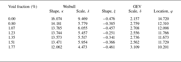
The results in figure 17 unveil that the impact pressures exhibit a degree of randomness during wedge water entry. Various probabilistic models have been developed to assess the uncertainties and variability of impact loads in different configurations (Hong et al. Reference Hong, Wei, Shen, Xu and Qin2021; Chuang Reference Chuang2022; Raby et al. Reference Raby, Bullock, Jonathan, Randell and Whittaker2022; Zhang et al. Reference Zhang, Xiao, Peng, Guo and Chen2024), while the probabilistic description of impact pressures on the wedge in aerated water entry has not been well understood. Therefore, a statistical analysis of the measured peak impact pressures under a range of void fractions was completed based on the two-parameter Weibull and generalised extreme value (GEV) distributions. The cumulative distribution function (CDF) of the two-parameter Weibull distribution is defined as
 \begin{equation} \begin{array}{c} F\left(x;\lambda ,\kappa \right)=1-\exp \left(-\left(\dfrac{x}{\lambda }\right)^{\kappa }\right),\end{array} \end{equation}
where
 $\lambda$
is the scale parameter and
 $\kappa$
is the shape parameter. Similarly, the CDF of the GEV distribution is written as
 \begin{equation} \begin{array}{c} G\left(x;\varphi ,\delta ,\xi \right)=\begin{cases} \exp \left(-\left[1+\xi \left(\dfrac{x-\varphi }{\delta }\right)\right]^{-{1}/{\xi }}\right), & \text{if }\xi \neq 0,\\[5pt] \exp \left(-\exp \left(-\dfrac{x-\varphi }{\delta }\right)\right), & \text{if }\xi =0, \end{cases} \end{array} \end{equation}
where
 $\varphi$
is the location parameter,
 $\delta$
is the scale parameter, and
 $\xi$
is the shape parameter.
The CDFs of the dimensionless peak pressures measured at sensors P01–P24 at various void fractions, along with the CDFs of the two fitted probability distributions with 95 % confidence intervals, are plotted in figures 18 and 19. (For brevity, the data for
 $\alpha =1.07\, \% ,1.23\mathrm{\, \% },1.35\mathrm{\, \% },1.51\mathrm{\, \% }$
are provided in the supplementary material.) Table 1 provides the parameter estimates for both two-parameter Weibull and GEV distributions for different void fractions. In general, both distributions gave a satisfactory description of the empirical distribution of the measured impact pressures. Notably, the shape parameter
 $\xi$
of the GEV distribution was negative, implying that the distribution represented the three-parameter Weibull distribution, belonging to the Weibull family. This suggested that the probability distribution of impact pressure during water entry under different void fractions followed a Weibull distribution.
The CDF of normalised pressure in pure water fitted with two-parameter Weibull and GEV distributions with 95 % confidence level based on the empirical CDF.

The CDF of normalised pressure in aerated water fitted with two-parameter Weibull and GEV distributions with 95 % confidence level based on the empirical CDF. The data for
 $\alpha =1.07\mathrm{\, \% },1.23\mathrm{\, \% },1.35\mathrm{\, \% },1.51\mathrm{\, \% }$
are provided in the supplementary material, shown in figure S2.

Parameter estimates for two-parameter Weibull and GEV distributions of normalised impact pressures under different void fractions.

It is observed that the shape parameter, particularly for the two-parameter Weibull distribution, displayed considerable variation for different
 $\alpha$
. This variation in the shape parameter highlighted the distribution’s sensitivity to the level of aeration. For the Weibull distribution, the scale parameter dropped sharply when a small amount of air (
 $\alpha =0.80\, \%$
) is introduced. A higher scale parameter generally reflects larger data values, while this sharp decline suggests that even a minor amount of aeration markedly reduces the peak impact pressure. Additionally, the location parameter of the GEV distribution tended to decrease with increasing void fraction, further indicating that the impact pressure diminished with higher void fractions. This aligned with the cushioning effect provided by the air bubbles, which mitigates the direct impact on the water surface, thereby reducing the peak pressure. The GEV scale parameter generally increased with the void fraction, reflecting a broader range in the distribution of peak impact pressures. This implied that the aeration introduced greater variability, as the presence of air bubbles resulted in a more dispersed distribution of measured impact pressures.
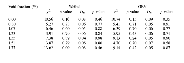
Typically, goodness-of-fit tests are implemented to assess the suitability of the selected probability distributions and to provide guidance for identifying the best-fitting distribution functions based on the established criteria. In this study, the fitting accuracies of the two distributions were assessed using both the weighted sum
 $\chi ^{2}$
of the chi-square (Chi-S) goodness-of-fit test and the supremum
 $D_{n}$
of the Kolmogorov–Smirnov (K–S) goodness-of-fit test. The
 $p$
-values for both tests were also calculated to strengthen the evidence for the appropriateness of these distributions. Detailed explanations of the two goodness-of-fit tests are provided in Appendix C. At significance level 0.05, the critical thresholds are
 $\chi ^{2}=14.067$
for Weibull,
 $\chi ^{2}=12.592$
for GEV, and
 $D_{n}=0.124$
for both distributions. Table 2 lists the weighted sum
 $\chi ^{2}$
and supremum
 $D_{n}$
results, along with their corresponding
 $p$
-values. Since both
 $\chi ^{2}$
and
 $D_{n}$
are below the critical values, and
 $p$
-values exceed 5 %, the null hypothesis is supported, confirming that both the GEV and Weibull distributions are suitable fits for the data. A larger
 $p$
-value suggests a better fit, given the same assumptions, confidence level and sample size. The
 $p$
-value for the GEV distribution is generally higher for most void fractions. While both distributions provide good overall fits, the GEV distribution shows slightly better performance under certain void fraction conditions.
Weighted sum
 $\chi ^{2}$
and supremum
 $D_{n}$
from the Chi-S and K–S goodness-of-fit tests for two probability distributions of normalised impact pressure with corresponding
 $p$
-value at different void fractions.

5. Conclusions
This study presents a detailed investigation into the influence of aeration on water entry impact pressures, using a novel application of the wire-mesh sensor (WMS) to measure void fractions in aerated water. Experiments were performed with a 20° deadrise angle wedge, dropped from height 750 mm into water with seven distinct void fractions. A custom-developed bubble generator, comprising 48 quartz sand-based porous boxes, ensured the introduction of small and uniform bubbles into the water. The experimental results were validated against theoretical models and prior experiments. The relationship between dimensionless peak pressure and void fraction was examined thoroughly. Additionally, a statistical analysis of the peak pressures was carried out to analyse the influence of aeration on impact pressure, offering new insights into the role of aeration in reducing and distributing impact loads.
The WMS was proved to be an effective tool for real-time measurement of void fractions, providing stable and consistent results under varied levels of aeration. Comparison with the image-based void fraction measuring method further confirmed the accuracy of the WMS. The flow visualisation of wedge water entry with different aeration levels highlights the significant influence of aeration on water entry dynamics, particularly on the development of water jets and splashes. The overall flow patterns remained consistent and repeatable for both pure and aerated water conditions. In pure water, the water jets formed symmetrical, coherent structures, whereas increasing void fractions introduced instability and chaotic jet patterns. Additionally, higher void fractions resulted in the displacement of jets and splashes, causing them to deviate from their vertical trajectory.
The comparison of maximum normalised peak pressures measured in this experiment with theoretical models (Wagner’s model and Mei’s model) and previous experimental results implied good agreement, validating the experimental findings. The deviations from Wagner’s model suggested that neglecting the compressibility of water and the air–water mixture can lead to an overestimation of impact pressures. This highlights the importance of considering air compressibility in aerated water impact studies.
The effects of aeration on the impact pressure during wedge water entry were evident in both the reduction of peak impact pressure and the extension of pressure duration. The peak pressures exhibited consistent reductions ranging from 15 % to 33 % as the aeration increased. The reduction is attributed to both the decreased density of the air–water mixture and the cushioning effect of air bubbles entrapped between the wedge and the water surface. This effect was further quantified through linear regression models, which consistently indicated a negative correlation between void fraction and peak pressure. The probability distribution of the peak impact pressures exhibited good fits with both the GEV and two-parameter Weibull distributions under a range of void fractions, as confirmed by Chi-S and K–S goodness-of-fit tests. Additionally, it was highly sensitive to the change in void fraction, particularly the shape parameter of the Weibull distribution.
This study provides a valuable experimental reference for examining the aerated water entry problem. However, one limitation is the potential variability in bubble size and distribution during wedge water entry process, despite the use of a carefully designed bubble generator. The motion of bubbles and induced fluid flows warrant future investigation to provide a more comprehensive understanding of the aerated water impact mechanisms. Furthermore, considering the impact of wedge entry on a wavy free surface is also crucial ((Zhao & Faltinsen Reference Zhao and Faltinsen1993) and provide link to this), and future research will focus on the variation in impact loads during wedge entry into aerated waves. In addition, the examined range of void fractions was limited by the experimental set-up, and future studies should explore a broader spectrum of aeration levels, as well as different gas–liquid mixtures.
Supplementary movies
Supplementary movies are available at https://doi.org/10.1017/jfm.2025.280.
Acknowledgements
The authors acknowledge Y. Chen for assisting with the experiment. They also wish to express their gratitude to Professor J. Xiong and Dr Y. Yang for their invaluable support.
Funding
This study is supported by the National Natural Science Foundation of China (grant no. 52031006).
Declaration of interests
The authors report no conflict of interest.
Appendix A. Overview of the WMS: principles and data processing methods
The WMS operates by measuring the electrical conductivity properties of the fluid, allowing for precise measurement of multiphase flows, particularly in gas–liquid systems. The sensor is composed of two orthogonally arranged planes of parallel wires, forming a grid where each wire crossing represents a virtual sensing point, as depicted in figure 20. In this configuration, one plane functions as the transmitter, while the other serves as the receiver. Typically, each plane consists of a grid of wires spaced 0.5–15 mm apart, which determines the spatial resolution (
 $d_{s}$
) of the measurements. The wires are made from materials with high conductivity and low resistance, ensuring accurate and responsive measurements. The transmitter and receiver planes are separated by a small axial distance, usually approximately 0.35–3 mm, which is crucial for maintaining the integrity of the electric field and reducing cross-talk between the wires.
Schematic overview of a typical WMS.

The detected current at each sensing point is amplified by transimpedance amplifiers, converting it into a voltage signal suitable for digitisation by an analogue-to-digital converter (ADC). The fluid conductance
 $G$
can be determined using the digital voltage
 $U_{m}$
with the equation
 \begin{equation} \begin{array}{c} G=\dfrac{U_{m}}{R_{oa}U_{T}},\end{array} \end{equation}
where
 $R_{oa}$
is the resistance associated with the transimpedance amplifier, and
 $U_{T}$
is the voltage sampled directly from the transmitter.
The data obtained by the WMS is a three-dimensional matrix of conductance (
 $G_{i,j,k}$
), where
 $(i, j)$
denotes the spatial positions of the electrodes, and
 $k$
is the time frame of data acquisition. Both
 $i$
and
 $j$
range from 1 to
 $N$
, with
 $N=64$
in this experiment. The primary task is to convert these conductance values into local void fractions that serve to quantify the proportion of gas in the two-phase flow. There are three primary conversion methods: the linear method, the Maxwell method, and the Bruggeman method. The linear approximation is the most commonly employed and is also adopted here, because the small grid spacing in WMS ensures that the phase between electrodes is expected to be entirely uniform (Tompkins, Prasser & Corradini Reference Tompkins, Prasser and Corradini2018). Since the conductivity of the gas is nearly zero, the conductance of the gas phase
 $G_{i, j}^{g}$
can be neglected compared to the liquid phase
 $G_{i, j}^{l}$
. The linear conversion equation is
 \begin{equation} \begin{array}{c} \alpha _{i,j,k}=\dfrac{G_{i,j}^{l}-G_{i,j,k}}{G_{i,j}^{l}-G_{i,j}^{g}}=1-\dfrac{G_{i,j,k}}{G_{i,j}^{l}},\end{array} \end{equation}
where
 $\alpha _{i,j,k}$
denotes the void fraction value at point
 $(i, j)$
and time
 $k$
, and
 $G_{i,j,k}$
is the corresponding conductance measured by the WMS. Here,
 $G_{i,j}^{l}$
represents the standard conductance of the liquid at the location
 $(i,j)$
, which is determined by the mean conductance value measured under pure water conditions at each point
 $(i,j)$
, accounting for local fluctuations in the distance between the wires.
The WMS provides real-time measurements at a high temporal resolution, which allows for the calculation of three important averaged void fractions to characterise the two-phase flow: the time-averaged void fraction, the spatially averaged void fraction, and the overall space–time averaged void fraction. The time-averaged void fraction at a given spatial location
 $(i, j)$
is obtained by averaging the instantaneous void fractions over all time frames:
 \begin{equation} \begin{array}{c} \overline{\alpha }_{i,j}=\dfrac{1}{M}\displaystyle\sum _{k=1}^{M}\alpha _{i,j,k},\end{array} \end{equation}
where
 $M$
is the total number of time frames. The spatially averaged void fraction at a given time frame
 $k$
is computed by averaging the void fractions across all grid locations:
 \begin{equation} \begin{array}{c} \alpha _{k}=\dfrac{1}{N\times N}\displaystyle\sum _{i=1}^{N} \sum _{j=1}^{N}\alpha _{i,j,k}.\end{array} \end{equation}
Finally, the space–time averaged void fraction, which gives a comprehensive representation of the two-phase flow over both time and space, is defined as
 \begin{equation} \begin{array}{c} \alpha =\dfrac{1}{M\times N\times N}\displaystyle\sum _{k=1}^{M} \sum _{i=1}^{N} \sum _{j=1}^{N}\alpha _{i,j,k}. \end{array} \end{equation}
Given the unavoidable noise, a filtering process is required prior to the utilisation of the raw data for the determination of the void fraction. A threshold-based segmentation method is employed, whereby noise signals are filtered out by applying a statistical criterion. In still pure water (actually tap water), the conductance data collected from each measurement points conform to a normal distribution, as exhibited in figure 21, where the conductance values have been normalised by the maximum measured conductance. From this distribution, the mean value
 $\mu$
and the standard deviation
 $\sigma$
are calculated. The mean value
 $\mu$
, which corresponds to the peak of the normal distribution curve, represents the standard conductance of the liquid
 $G_{i, j}^{l}$
at the location
 $(i, j)$
. According to the Pauta criterion, the probability of noise occurring outside the range
 $[\mu -3\sigma , \mu +3\sigma ]$
is negligible, making it statistically improbable. As a result, when conductance values exceed
 $\mu -3\sigma$
, they are treated as the standard conductance of pure water
 $G_{i, j}^{l}$
, corresponding to void fraction 0. Only conductance values below
 $\mu -3\sigma$
are considered valid and representative of true measurements, effectively eliminating the influence of noise. The filtered conductance values are then processed using the function
Histogram of the normalised conductance at a measuring point in pure water. The conductance values have been normalised by the maximum measured conductance. The red line denotes the fitted normal distribution.

 \begin{equation} \begin{array}{c} G_{i,j,k}^{\prime}=\begin{cases} G_{i,j,k}, & \mathrm{if}\ G_{i,j,k}\leq \mu -3\sigma, \\ G_{i, j}^{l}, & \mathrm{if}\ G_{i,j,k}\gt \mu -3\sigma. \end{cases} \end{array} \end{equation}
This approach guarantees that any conductance values above the threshold are discarded as noise, while the values within the acceptable range are retained as accurate data. Figure 22 displays a comparison of the void fraction distributions before and after the noise filtering process, demonstrating the effectiveness of this method in refining the measurements.
Comparison between the original and denoised void fraction distributions.

Appendix B. Mei’s analytical model of impact pressure coefficient for wedge water entry
Mei’s analytical model (Mei et al. Reference Mei, Liu and Yue1999) provided an advanced method for calculating the pressure coefficient
 $C_{P}$
during wedge water entry by improving the classical approaches. By employing the Schwartz–Christoffel transformation, the complex problem of flow around a wedge was simplified, allowing for the analytical determination of the pressure distribution along the wedge’s surface. The accuracy of Mei’s model in predicting the maximum values of pressure coefficient
 $C_{P_{max}}$
was confirmed by Yettou et al. (Reference Yettou, Desrochers and Champoux2006).
The model is expressed by the following formula for the pressure coefficient
 $C_{P}$
:
 \begin{equation} \begin{array}{rl} C_{P}&=\dfrac{2\gamma }{A\tan \left(\beta \right)}\left[\left(\dfrac{1-q^{2}}{q^{2}}\right)^{\theta }\displaystyle\int _{\left| q\right| }^{1}\left(\frac{w^{2}}{1-w^{2}}\right)^{\theta }\mathrm{d}w-q\right]\\ &\quad -\left(\dfrac{1-q^{2}}{q^{2}}\right)^{2\theta }-2\gamma +1,\quad \theta =\dfrac{{\unicode{x03C0}} -2\beta }{2{\unicode{x03C0}} }, \end{array} \end{equation}
where
 $\beta$
denotes the deadrise angle of the wedge, and the real variable
 $q$
is defined in (B4). The splash-up coefficient
 $\gamma$
, which measures the rise of the water surface on the body relative to its submergence
 $Vt$
, is calculated as
 \begin{equation} \begin{array}{c} \gamma \left(\beta \right)=A\displaystyle\int _{0}^{\mathrm{\infty }}\left[\int _{0}^{p}\left(\dfrac{w^{2}}{w^{2}+1}\right)^{\theta }\mathrm{d}w+A\right]^{-2}\mathrm{d}p. \end{array} \end{equation}
For a wedge with
 $\beta =0$
,
 $\gamma ={\unicode{x03C0}} /2$
, it aligns with Wagner’s asymptotic solution for small deadrise angles. For
 $\beta ={\unicode{x03C0}} /2$
,
 $\gamma =1$
, it is the solution of von Karman in the limit of no splash-up. The coefficient
 $A$
, which is crucial for evaluating the pressure distribution around the wedge during water entry, is derived from the conformal mapping process that transforms the complex flow in the physical plane into a more manageable form in the mapped plane. It is obtained through the following integral equation, which accounts for the geometry of the wedge and the deadrise angle
 $\beta$
:
 \begin{equation} \begin{array}{c} A\left(\beta \right)=\cos \left(\beta \right)\displaystyle\int _{0}^{1}\left(\dfrac{w^{2}}{1-w^{2}}\right)^{\theta }\mathrm{d}w. \end{array} \end{equation}
In (B1), the real variable
 $q$
is related to the position on the body by
 \begin{equation} \begin{array}{c} \dfrac{h\left(y\right)}{Vt}=\gamma A^{-1}\cos \alpha \displaystyle\int _{0}^{q}\left(\dfrac{w^{2}}{1-w^{2}}\right)^{\theta }\mathrm{d}w+\gamma ,\quad \text{for }0\leq \dfrac{h\left(y\right)}{Vt}\leq \gamma. \end{array} \end{equation}
The term
 $h(y)$
denotes the vertical coordinate of the intersection between the wedge surface and the free water surface.
Mei’s model effectively addresses the complex hydrodynamics involved in wedge water entry by considering the conformal mapping of the flow field, accounting for the wetted surface dynamics and the influence of splash-up effects. By applying these equations, the maximum pressure coefficient
 $C_{P_{max} }$
at any point on the wedge surface can be determined, offering an essential tool for predicting the impact loads in the water entry problem.
Appendix C. The Chi-S and K–S goodness-of-fit tests
In this study, the Chi-S and K–S goodness-of-fit tests were employed to assess the accuracy of the fitted probability distributions against the experimental data.
C.1 The Chi-S goodness-of-fit test
The Chi-S goodness-of-fit test is a statistical method used to evaluate the degree of agreement between observed and expected frequencies (Kottegoda & Rosso Reference Kottegoda and Rosso1997). It is particularly useful for categorical data and large sample sizes (each category should not be less than 5), where the distribution of observed values can be compared with an expected theoretical distribution. The test is based on the Chi-S statistic (
 $\chi ^{2}$
), which can be expressed as
 \begin{equation} \begin{array}{c} \chi ^{2}=\displaystyle\sum _{z=1}^{M_{c}}\frac{\left({O_{z}}-{E_{z}}\right)^{2}}{E_{z}}, \end{array} \end{equation}
where
 $O_{z}$
is the observed frequency, and
 $E_{z}$
is the expected frequency, for category
 $z$
, and
 $M_{c}$
is the total number of categories. The sum of squared deviations is normalised by the expected frequency to account for the magnitude of each category. To determine whether the observed data deviate significantly from the hypothesised distribution, the test compares the computed
 $\chi ^{2}$
value against a critical value from the Chi-S distribution, depending on the degrees of freedom (
 $\nu$
) and significance level (
 $\alpha ^{\prime}$
). The degrees of freedom are determined by
 \begin{equation} \begin{array}{c} \nu =M_{c}-1-\varepsilon, \end{array} \end{equation}
where
 $\varepsilon$
is the number of estimated parameters (
 $\varepsilon =2$
for the two-parameter Weibull distribution, and
 $\varepsilon =3$
for the GEV distribution).
The null hypothesis assumes no significant difference between the observed and expected frequencies. If the computed
 $\chi ^{2}$
value is less than the critical value corresponding to a given significance level (e.g.
 $\alpha ^{\prime}=0.05$
), then the null hypothesis cannot be rejected, indicating a good fit. The corresponding
 $p$
-value is also computed to provide an additional measure of fit quality, and if it exceeds 0.05, then it indicates that the null hypothesis can be accepted. Additionally, under the same assumptions, a larger
 $p$
-value suggests a better fit between the observed and expected distributions.
C.2 The K–S goodness-of-fit test
The K–S test is a non-parametric test that assesses the degree of agreement between the empirical CDF of the sample data and the theoretical CDF of the proposed distribution (Parsons & Wirsching Reference Parsons and Wirsching1982). It is particularly useful when comparing continuous distributions, and does not require binning of data.
The K–S statistic
 $D_{n}$
is defined as the maximum absolute difference between the empirical CDF
 $F_{n}(x)$
and the theoretical CDF
 $F_{0}(x)$
:
 \begin{equation} \begin{array}{c} D_{n}=\underset{x_{z}}{\sup }|F_{n}\left(x\right)-F_{0}\left(x\right)|.\end{array} \end{equation}
For a given significance level (
 $\alpha ^{\prime}$
), the critical value of
 $D_{n,\alpha ^{\prime}}$
can be determined by
 \begin{equation} \begin{array}{c} D_{n,\alpha ^{\prime}}=\dfrac{1.36}{\sqrt{N_{s}}},\end{array} \end{equation}
where
 $N_{s}$
is the sample size (no less than 40). The null hypothesis is that the sample comes from the hypothesised distribution. If
 $D_{n}$
is less than the critical value, then the null hypothesis cannot be rejected, and the distribution is considered a good fit. As with the Chi-S test, the
 $p$
-value is also calculated to assess the probability of observing a test statistic as extreme as
 $D_{n}$
under the null hypothesis. Larger
 $p$
-values indicate a better fit between the empirical and theoretical distributions.
Both goodness-of-fit tests are applied to the data under varying void fractions to evaluate the suitability of the Weibull and GEV distributions. By assessing the values of
 $\chi ^{2}$
,
 $D_{n}$
, and their corresponding
 $p$
-values, it is possible to quantify the accuracy of the fitted distributions and determine which model best captures the statistical properties of the impact pressures.