





1. Introduction
The Graded Ring Database, or Grdb, is a collection of data that relates to polarized varieties and their graded rings. The motivation for such a database is founded on various celebrated finiteness results for Fano varieties [Reference Birkar12], [Reference Kawamata68], [Reference Kollár, Miyaoka, Mori and Takagi69]. Fano varieties are among the key elementary particles of geometry, and here we are interested specifically in Fano
$3$
 -folds over
$\mathbb C$
 . Nonsingular Fano
$3$
 -folds are classified into 105 families [Reference Iskovskikh58], [Reference Mori and Mukai75] and are recorded with additional data both in print [Reference Iskovskikh and Prokhorov59] and online [Reference Belmans11]. The nonsingular Fanos form a kind of aristocracy, making them a popular topic for certain authors. However, the broad toiling masses of Fano
$3$
 -folds with terminal singularities are not to be neglected, and their study offers rich rewards. Several hundred families of them are already known (see §4), with the reasonable expectation of thousands or tens of thousands more yet to be discovered—and orders of magnitude more if we relax the conditions on singularities further. Ultimately, if ever completed, the classification will be a computer database rather than a physical atlas. The Grdb is a first approximation to that database. In the meantime, it provides a roadmap for exploring the landscape, and for identifying candidates for construction or elimination.
It is a key point that, while not huge, the data are too large to be written down usefully, and alternative access is vital. The easiest way to access and interrogate the Fano
$3$
 -fold database (the data described precisely in 2.9) is online at [Reference Brown and Kasprzyk22]; some form of this data access has been online for over 25 years since [Reference Altınok, Brown and Reid3]. The underlying raw data are available at [Reference Brown and Kasprzyk25] in generic SQL format. Code to generate the data is at [Reference Brown and Kasprzyk22] (for Magma [Reference Bosma, Cannon and Playoust13]) and [Reference Brown and Kasprzyk24] (for Go [Reference Cox, Griesemer, Pike, Taylor and Thompson48]).
Two main considerations govern our view of Fano 3-folds (or
${\mathbb {Q}}$
 -Fano 3-folds) and the precise terminology we use here. Prime Fano
$3$
 -folds (see Definition 1.3) form the strictest class. They have a distinguished place in the birational classification of
$3$
 -folds: each one is the endpoint of a minimal model program (MMP) in the Mori category [Reference Mori74, Theorem 0.3.1]. On the other hand, the main numerical invariant of a Fano variety that we use is its anticanonical Hilbert series (§2.1) and the ingredients that go into it (§2.2). This is the basic object of the Grdb and it works for a much broader definition allowing canonical singularities (see Definition 1.1). For varieties with worse than canonical singularities, this viewpoint breaks down, even for mild log terminal orbifold points. Throughout this article, we say 3-fold to mean a normal variety of dimension 3 over
$\mathbb C$
 .
Definition 1.1. A Fano 3-fold with canonical singularities is a projective
$3$
 -fold X with at worst canonical singularities, for which the anticanonical class
$-K_X$
 is ample. We usually abbreviate “Fano
$3$
 -fold with canonical singularities” to “Fano
$3$
 -fold.” By definition, the genus of X is
$g_X := h^0(X,-K_X)-2$
 .
In [Reference Kollár, Miyaoka, Mori and Takagi69], this class is called canonical
${\mathbb {Q}}$
 -Fano 3-folds and it is shown to be bounded [Reference Kollár, Miyaoka, Mori and Takagi69, 1.3]. The point of the Grdb is to realize this bound explicitly under stated conditions. Our main result is a list
${\mathcal F}_{3}$
 of rational functions (defined in Definition 2.9) that satisfy necessary conditions to be the Hilbert series of a Fano
$3$
 -fold (polarized by
$-K_X$
 as in §2.2), subject to an additional numerical condition.
Theorem 1.2. Let X be a Fano
$3$
 -fold satisfying
$-K_X^3\le -3K_Xc_2$
 . Then its Hilbert series
$P_X(t)$
 is one of the
$39,\!550$
 rational functions in the list
${\mathcal F}_{3}$
 .
The condition
$-K_X^3\le -3K_Xc_2$
 is natural, as we discuss further below. Our use of it is motivated by the proof of Kawamata’s boundedness theorem [Reference Kawamata68], one of the earliest for
$3$
 -folds, and one which seems well suited to explicit classification in a range of contexts.
Definition 1.3 (Prime Fano 3-fold)
The Mori category consists of
$3$
 -folds X with
${\mathbb {Q}}$
 -factorial terminal singularities. We say that a 3-fold X in the Mori category is a prime Fano 3-fold if
$-K_X$
 is ample, and the Weil divisor class group
$\operatorname {\mathrm {Cl}} X$
 has rank
$\rho _X=1$
 .
Here, we intend
${\mathbb {Q}}$
 -factorial in the algebraic sense: the local ring
$\mathscr O_{X,P}$
 at every
$P\in X$
 is
${\mathbb {Q}}$
 -factorial, or equivalently, any algebraic Weil divisor on X has a multiple that is Cartier. The complex analytic variety
$X^{\mathrm {an}}$
 may not be
${\mathbb {Q}}$
 -factorial in the local or étale analytic setting: as an example, a cubic or quartic 3-fold hypersurface
$X\subset \mathbb {P}^4$
 with a single ordinary node is
${\mathbb {Q}}$
 -factorial, although the node is (analytic, étale, or formal)-locally isomorphic to
$xy=zt$
 .
On the other hand, we do not insist that
$-K_X$
 generates the class group
$\operatorname {\mathrm {Cl}} X$
 : we allow
$-K_X\in \operatorname {\mathrm {Cl}} X$
 to be divisible (see Definition 2.1 below for a discussion of index), and
$\operatorname {\mathrm {Cl}} X$
 may have a finite torsion group.
Prime Fano
$3$
 -folds remain unclassified. The proof of [Reference Kawamata68, Proposition 1] determines inequalities on prime Fano
$3$
 -folds of the form
${-}K_X^3\le {-}\unicode{x3ba} K_Xc_2(X)$
 for certain values of
$\unicode{x3ba}>0$
 . These in turn impose numerical constraints on the Hilbert series
$P_{X}$
 of X. A Fano
$3$
 -fold X is Bogomolov semistable if the sheaf
${\mathcal E}=({\Omega ^1_X})^{\vee \vee }$
 is semistable. Kawamata shows that for prime semistable X, the inequality above holds with
$\unicode{x3ba} =3$
 as in Theorem 1.2; it follows at once from the Bogomolov–Miyaoka–Yau inequality
$c_1^2\le 3c_2$
 applied to
${\mathcal E}$
 restricted to suitable
$S\in |{-}RK_X|$
 for large divisible R.
More recently, Liu and Liu [Reference Liu and Liu73, Theorem 1.3] prove that the strict inequality
${-}K_X^3 < -3K_Xc_2(X)$
 holds for any prime Fano
$3$
 -fold with terminal singularities (cf. [Reference Suzuki97]), and so Theorem 1.2 applies in this case. Only 208 of the 39,550 candidates fail this strict inequality, and none of these 208 is currently realized.
Corollary 1.4. If X is a prime Fano
$3$
 -fold, then
$P_X\in {\mathcal F}_{3}$
 .
In fact,
${\mathcal F}_3$
 contains almost all Fano
$3$
 -folds we know. Most series in
${\mathcal F}_3$
 are not the Hilbert series of a prime Fano
$3$
 -fold: the main issue is to begin to understand which ones are, which ones are realized by more general classes of Fano
$3$
 -fold, and which ones are not realized by Fano
$3$
 -folds at all.
Relaxing
$\unicode{x3ba} =3$
 to
$\unicode{x3ba} =4$
 accommodates most of Kawamata’s conditions even in the non-semistable case (see Theorem 2.7). Imposing only that weaker condition gives a larger list
${\mathcal F}_{4}$
 of
$52,\!646$
 rational functions that contains
${\mathcal F}_{3}$
 (see Proposition 2.10). Liu and Liu [Reference Liu and Liu72, Theorem 1.1] also prove that if X is a Fano
$3$
 -fold with
$\rho _X=1$
 which is nonsingular in codimension 2, then it satisfies the strict inequality
$-K_X^3 < -4K_Xc_2$
 . Only 87 of the
$52,\!646$
 fail this strict inequality.
Corollary 1.5. If X is a Fano
$3$
 -fold with isolated canonical singularities and
$\rho _X=1$
 , then
$P_X\in {\mathcal F}_{4}$
 .
For example, the weighted projective space
$\mathbb {P}(1,1,3,5)$
 lies in
${\mathcal F}_{4}\setminus {\mathcal F}_{3}$
 . It has Picard rank
$\rho =1$
 , but is not prime because it has the mild canonical singularity
$\tfrac {1}5(1,1,3)$
 .
Definition 1.6 (cf. Definition 2.9)
The Fano 3-fold database is the pair of lists
${\mathcal F}_{3}\subset {\mathcal F}_{4}$
 . We say that a Fano
$3$
 -fold X is in
${\mathcal F}_{3}$
 when
$P_X\in {\mathcal F}_{3}$
 . The Fano
$3$
 -fold database may be accessed online [Reference Brown and Kasprzyk22] and the raw data are available at [Reference Brown and Kasprzyk25] under a CC0 licence [49].
The Grdb also includes the data of all toric Fano
$3$
 -folds, so it is easy to derive the following.
Proposition 1.7 (§4.5 and Table 6)
The
$674,\!688$
 toric Fano
$3$
 -folds realize
$5772$
 different Hilbert series. If X is a toric Fano
$3$
 -fold, then
$P_X\in {\mathcal F}_{4}$
 , and
$5760$
 of these Hilbert series lie in
${\mathcal F}_{3}$
 .
We emphasize that some unknown, and possibly significant, fraction of the elements of
${\mathcal F}_{3}$
 cannot be realized as the Hilbert series of a Fano
$3$
 -fold (see §5.3 for a recapitulation of this point and §5.1 for several other possible confusions).
We explain the proof of Theorem 1.2 in §2.4. This may be thought of as folklore, and similar in spirit to Prokhorov’s degree bound computation [Reference Prokhorov85, (1.2)]. Nevertheless, the steps turning Kawamata’s theorem into a concrete list are important in light of the bounds on Fano varieties more generally. The main results of this article supplement 1.2 as follows:
-
1. For each $P\in {\mathcal F}_{3}$
 , we estimate the smallest anticanonical embedding that a Fano
$3$
-fold X with Hilbert series
$P_X=P$
could have (§3), and we use those to present
${\mathcal F}_{3}$
as a geographical map of candidates (Table 1). This geography, and its meaning as the basis for a program of classification, is the main result of this article.Table 1
Number of semistable Fano $3$
-fold Hilbert series in
${\mathcal F}_{3}$
, listed by genus and estimated minimal codimensionTable 1 Long description
The table categorizes 39,550 Hilbert series based on Genus (horizontal axis) and Codimension (vertical axis).
* Genus Axis: Values range from negative 2 to 37. Key columns include negative 2, negative 1, 0, 1, 2, 7, 12, 17, 22, 27, 32, and 37.
* Codimension Axis: Values range from 1 to 35.
* Data Distribution:
- The highest concentrations are found at low Codimension and low Genus. For example, Codimension 18 has a total of 4,709 series, and Codimension 17 has 4,696.
- Genus 0 contains 6,166 series, the highest for any single genus.
- As Genus increases, the distribution shifts toward higher Codimension values, creating a diagonal trend from the top-left toward the bottom-right.
- For Codimension 1, the series are concentrated between Genus negative 1 (54) and Genus 3 (1).
- For Codimension 35, there is only 1 series located at Genus 37.
* Totals:
- The bottom row shows total series per Genus, peaking at Genus 0 (6,166) and tapering to 1 at Genus 37.
- The rightmost column shows total series per Codimension, peaking at Codimension 18 (4,709) and tapering to 1 at Codimension 35.
- The grand total is 39,550.
-
2. We identify some known classifications within the Fano $3$
-fold database (§4) and compare with some well-known results (§3.3). -
3. We highlight possible misunderstandings of the Fano $3$
-fold database (§§5.1 and 5.3). -
4. The numbers of cases $\#{\mathcal F}_{3}=39,\!550$
and
$\#{\mathcal F}_{4}=52,\!646$
arise from elementary combinatorial considerations (Proposition 2.10).


In outline, §2 constructs the lists
${\mathcal F}_{3}$
 and
${\mathcal F}_{4}$
 , §3 explains the estimates of codimension that lead to Table 1, §4 describes a number of constructions and comparisons with known lists of Fano
$3$
 -folds, and finally §5 summarizes the Grdb together with important warnings about its meaning.
We put some emphasis on toric Fano
$3$
 -folds throughout, in part to profit from simultaneous use of the Fano
$3$
 -fold database and the toric Fano classification in the Grdb. We indicate in §4.5 some different ways that this interdisciplinary approach may yet be exploited.
The systematic study of the graded rings of all Fano
$3$
 -folds together in this way was initiated by Miles Reid (see [Reference Altınok, Brown and Reid3]), which alongside [Reference Altınok2], [Reference Iano-Fletcher56], was the starting point for the Grdb. The Grdb has been available since then in different forms [Reference Brown and Kasprzyk22], [Reference Brown and Kasprzyk25], though without the documentation and detailed analysis this article provides. The need for this analysis has become more important recently, as a series of developments promise to expose large new parts of the classification:
-
• The use of formats by Takagi [Reference Takagi101], [Reference Takagi106], [Reference Takagi107] and Coughlan–Ducat [Reference Coughlan and Ducat47] extends the cases of [Reference Brown, Kasprzyk and Qureshi26], [Reference Brown, Kasprzyk and Zhu27] (§4.6) and opens up mid-range codimension to similar analysis.
-
• New Kawamata–Miyaoka inequalities [Reference Liu and Liu72] provide sharper data in broader contexts (cf. Corollaries 1.4 and 1.5) and also higher dimension.
-
• Variations of the Papadakis–Reid unprojection techniques exploited in [Reference Brown, Kerber and Reid28] provide constructions for many more families [Reference Brown, Coughlan, Ducat and Cheltsov19], [Reference Brown, Coughlan and Ducat20], [Reference Petrotou82], [Reference Taylor109].
-
• The Fanosearch programme [Reference Brown, Coates, Corti, Ducat, Heuberger, Kasprzyk, He, Ge, Bai, Bao and Hirst17], [Reference Coates, Corti, Galkin, Golyshev and Kasprzyk38] (§4.8) attacks classification via Mirror Symmetry, exploiting certain types of degeneration; thus, as a first approximation, the raw Grdb list is supplemented by matching toric Fano $3$
-folds, which are classified (§4.5).

This article makes the Grdb precise: it provides the theorems that underpin the data and its construction, it relates the data to a range of classical results, and by locating a class of toric varieties within the data, it provides a first step in identifying certain degenerations. There is a quick startup guide in §5, which also summarizes the essential warnings for its use.
The beauty and enduring interest of Fano classification lies in the individual
$3$
 -folds and deformation families we meet, rather than the bureaucracy of compartmentalizing them. A map is only a map: the actual adventures happen out in the field. The real value of the geography in Table 1 is to identify hundreds of wonderful places to explore: compare [Reference Brown, Kerber and Reid28], [Reference Corti, Haskins, Nordström and Pacini44], [Reference Coughlan and Ducat47], [Reference Di Natale, Fatighenti and Fiorenza50], [Reference Heuberger55], [Reference Süss95], [Reference Takagi103].
2. Building the Fano 3-fold database
We recall standard material related to the plurigenus formula and use it to assemble the data that proves Theorem 1.2 (cf. [Reference Altınok, Brown and Reid3, §4]).
2.1. Fano 3-folds
Any Fano
$3$
 -fold X comes with an intrinsic embedding
$X\subset w\mathbb {P}$
 in weighted projective space (up to automorphisms of
$w\mathbb {P}$
 ) as follows. The graded ring of X is

and
$X\cong \operatorname {\mathrm {Proj}} R(X,-K_X)$
 by ampleness. Any choice
$f_0,\dots ,f_n$
 of minimal homogeneous generators for
$R(X,-K_X)$
 has the same collection of weights
$\{a_0,\dots ,a_n\}$
 , where
$a_i=\deg f_i$
 , and we may suppose
$a_0\le \cdots \le a_n$
 . (Note the conventional abuse of notation:
$\{a_0,\dots ,a_n\}$
 is a list with possible repetitions, and similarly
$\{a_0,\dots ,a_n\}\setminus \{a_3,a_7\}$
 is the list obtained by removing one instance of each of
$a_3$
 and
$a_7$
 ). Thus, any choice of a minimal generating set determines a projectively normal embedding

which we refer to as the anticanonical embedding of X. (This is not the same as the image
$\Phi _{-K_X}(X)$
 under the linear system
$|{-}K_X|$
 unless
$-K_X$
 is very ample, which is rarely the case here).
The Hilbert series
$P_X$
 of a Fano
$3$
 -fold X is simply that of
$R(X,-K_X)$
 , the formal power series

The Hilbert series
$P_X$
 of a Fano
$3$
 -fold X does not determine the weights
$a_i$
 of its anticanonical embedding—it not infrequently happens that
$R(X,-K_X)$
 has relations and generators in the same degree.
2.2. Numerical data of a Fano 3-fold
We write
$\tfrac {1}r(a_1,a_2,a_3)$
 to denote the singularity germ of the origin in
$\mathbb C^3/\boldsymbol \mu _r$
 , where
$\boldsymbol \mu _r$
 is the multiplicative group of rth roots of unity, and
$\varepsilon \in \boldsymbol \mu _r$
 acts on coordinates by
$(\varepsilon ^{a_1}x_1,\varepsilon ^{a_2}x_2,\varepsilon ^{a_3}x_3)$
 . Any Fano
$3$
 -fold has a basket of singularities
${\mathcal {B}}$
 , which is a collection of terminal quotient singularities
$\tfrac {1}{r}(1,a,-a)$
 (possibly including repeats, where again we use set notation on this understanding). Following [Reference Reid89, §§8–10], in general,
${\mathcal {B}}$
 is derived locally from the singularities of X by crepant blowup and Q-smoothing. When X has terminal singularities and lies in a weighted projective space as a quasismooth variety, then X is an orbifold and
${\mathcal {B}}$
 is exactly the collection of singularities of X.
The genus
$g=h^0(X,-K_X)-2\ge -2$
 and basket
${\mathcal {B}}$
 together determine the degree by the formula

where for each element
$\tfrac {1}{r}(1,a,-a)$
 of the basket
${\mathcal {B}}$
 , we define
$0<b<r$
 by
$ab\equiv 1\mod r$
 .
Although they are not used for the initial construction of the Grdb, there are various different divisorial indices defined for a Fano
$3$
 -fold X that we consider later.
Definition 2.1. The Gorenstein index or singularity index of X is

The Fano index is the rational number
$f_X = r/i_X$
 , where
$r>0$
 is the largest integer for which
$-i_X K_X \equiv rA$
 for a Cartier divisor A. There are further types of Fano index:

These are natural generalizations of the divisibility of the anticanonical divisor of a nonsingular Fano
$3$
 -fold in its Picard group. For a Fano
$3$
 -fold, both q and
$q_{\mathbb {Q}}$
 are positive integers, and they are equal if
$\operatorname {\mathrm {Cl}}(X)$
 has no torsion [Reference Prokhorov83].
2.3. Effective Kawamata bounds for prime Fano 3-folds
We construct the set of genus–basket pairs
$(g,{\mathcal {B}})$
 that satisfy the constraints of [Reference Kawamata68].
2.3.1. Possible baskets
Controlling the possible baskets of Fano
$3$
 -folds can be done much more generally than the prime Fano case. Recall that a basket
${\mathcal {B}}$
 is a set with possible repeats.
Definition 2.2. We fix a particular set
$\mathbb B$
 of baskets
${\mathcal {B}}$
 as
$\mathbb B = \left \{ {\mathcal {B}} \mid \sum _{{\mathcal {B}}} (r - \frac {1}{r}) < 24 \right \}$
 , where each
${\mathcal {B}}$
 is a basket and the sum is taken over the quotient singularities
$\tfrac {1}r(1,a,-a)\in {\mathcal {B}}$
 .
It is elementary and easy to check that
$\#\mathbb B = 8{,}314$
 . For any
${\mathcal {B}}\in \mathbb B$
 , the defining bound of 24 implies first that
$r\le 24$
 for each
$\tfrac {1}r(1,a,-a)\in {\mathcal {B}}$
 , and moreover that
$\#{\mathcal {B}}\le 15$
 , since each
$r-(1/r) \ge 3/2$
 . Therefore, there are only finitely many possible collections of indices r appearing in
${\mathcal {B}}$
 . The only terminal quotient singularity with
$r=2$
 is
$\tfrac {1}2(1,1,1)$
 , and for each index
$r>2$
 , there are
$\phi (r)/2$
 distinct terminal quotient singularities, namely,
$\tfrac {1}r(1,a,-a)$
 for
$1\le a< r/2$
 coprime to r. Thus, for each index r that appears in
${\mathcal {B}}$
 , there are only finitely many singularities of index r that may occur. The precise bound 8,314 comes by enumerating all possible baskets satisfying these conditions (by computer, for example).
Theorem 2.3 [Reference Kawamata67, Lemmas 2.2 and 2.3] and [Reference Reid89, (10.3)]
Let X be a projective
$3$
 -fold with canonical singularities. Then

where the sum is over the singularities
$\tfrac {1}r(1,a,-a)$
 of the basket
${\mathcal {B}}$
 of X.
When X is a Fano
$3$
 -fold,
$\chi (\mathscr O_X)=1$
 and (2.C) simplifies.
Lemma 2.4. If X is a Fano
$3$
 -fold with canonical singularities which satisfies
$-K_X c_2(X)> 0$
 , then the basket
${\mathcal {B}}$
 of X is in
$\mathbb B$
 .
Proof. The condition
$-K_X c_2(X)> 0$
 together with (2.C) implies that
$\sum r - (1/r) < 24$
 , where the sum is taken over the basket
${\mathcal {B}}$
 .
Remark 2.5. The condition
$-K_Xc_2(X)>0$
 holds for prime Fano
$3$
 -folds by Theorem 2.7. Far more generally, any weak Fano
$3$
 -fold (i.e.,
$-K_X$
 is only required to be nef and big) with terminal singularities satisfies
$-K_Xc_2(X)\ge 0$
 by [Reference Kollár, Miyaoka, Mori and Takagi69, 1.2(1)]. It is easy to check that relaxing the inequality provides (coincidentally) 24 additional cases with
$\sum r-(1/r)=24$
 , such as
$16\times \tfrac {1}2(1,1,1)$
 and
$5\times \tfrac {1}5(1,2,3)$
 .
2.3.2. Genus bounds
Controlling the possible values for the genus
$g_X$
 for each basket uses the bounds determined by [Reference Kawamata68].
Proposition 2.6. Let X be a Fano
$3$
 -fold with basket
${\mathcal {B}}$
 and genus g that satisfies

for some
$\unicode{x3ba}>0$
 . Then
$g_{\mathrm {min}} \le g \le g_{\mathrm {max}}$
 where

and

where each sum is over
$\tfrac {1}r(1,a,-a)\in {\mathcal {B}}$
 and b is defined by
$ab\equiv 1\mod r$
 .
Proof. The lower bound is simply the condition that
$-K_X^3>0$
 in (2.B). For the upper bound, substituting (2.B) and (2.C) into (2.D) gives

and the upper bound follows.
Theorem 2.7 (Kawamata [Reference Kawamata68])
Let X be a prime Fano
$3$
 -fold. Then

for some real number
$\unicode{x3ba}>0$
 . In particular,
$-K_X c_2(X)> 0$
 .
If X is semistable, then the formula (2.E) holds with
$\unicode{x3ba} =3$
 . If
$(\Omega _X^1)^{\vee \vee }$
 has a rank
$2$
 maximal destabilizing subsheaf, then the formula holds with
$\unicode{x3ba} =4$
 . If
$(\Omega _X^1)^{\vee \vee }$
 has a rank
$1$
 maximal destabilizing subsheaf, then it holds with possibly larger
$\unicode{x3ba}>0$
 .
2.4. Proof of 1.2
The Hilbert series
$P_X$
 is equivalent to the data of genus–basket pair
$(g,{\mathcal {B}})$
 by the following Fletcher–Reid plurigenus formula together with (2.B) and the independence of basket contributions [Reference Fletcher52, 4.2]. We could instead use the integral orbifold Riemann–Roch formulas of [Reference Buckley, Reid and Zhou32], and for human calculation they are much preferred.
Theorem 2.8 [Reference Fletcher51, Theorem 2.5] and [Reference Reid89, (10.3)]
Let X be a Fano
$3$
 -fold with canonical singularities and basket
${\mathcal {B}}$
 . Then

where for each element
$\tfrac {1}{r}(1,a,-a)$
 of the basket
${\mathcal {B}}$
 , we fix any integer b that satisfies
$ab\equiv 1\mod r$
 , and set
$\overline {bi}\in \{0,1,\ldots ,r-1\}$
 to be the least residue of
$(bi)$
 modulo r.
Definition 2.9. For any
$g\ge -2$
 and
${\mathcal {B}}\in \mathbb B$
 , the right-hand side of (2.F) determines a rational function that we denote
$P_{g,{\mathcal {B}}}$
 , where (2.B) expresses the
$-K_X^3$
 factor in terms of
$g,{\mathcal {B}}$
 . We may expand
$P_{g,{\mathcal {B}}} = \sum P_nt^n$
 as a power series, and conversely, given such a power series, we may recover
$g,{\mathcal {B}}$
 and the expression (2.F) as a rational function. For any
$\unicode{x3ba}>0$
 , define

where
$g_{\mathrm {min}}$
 and
$g_{\mathrm {max}}$
 are defined for
${\mathcal {B}}$
 by (2.E) with the given
$\unicode{x3ba} $
 . We treat
${\mathcal F}_\unicode{x3ba} $
 as a set of genus–basket pairs, or equivalently as a set of rational functions they determine, and we write
$(g,{\mathcal {B}})\in {\mathcal F}_\unicode{x3ba} $
 or
$P_{g,{\mathcal {B}}}\in {\mathcal F}_\unicode{x3ba} $
 accordingly.
It follows from everything so far that if X is a Fano
$3$
 -fold with genus g and basket
${\mathcal {B}}$
 that satisfies (2.D) for
$\unicode{x3ba}>0$
 , then
$P_X=P_{g,{\mathcal {B}}}\in {\mathcal F}_{\unicode{x3ba} }$
 . The condition on
$P_n$
 holds for any such
$P_X$
 : there cannot be a nonzero section
$x\in H^0(X,-K_X)$
 with
$x^n=0$
 for some
$n>1$
 .
Proposition 2.10.
$\#{\mathcal F}_{3}=39,\!550$
 and
$\#{\mathcal F}_{4}=52,\!646$
 .
Proof. Lemma 2.4 provides exactly
$8{,}314$
 possible baskets. Of these, (2.E) calculates
$g_{\mathrm {max}}\ge -2$
 in
$7{,}492$
 cases for
$\unicode{x3ba} =3$
 and in
$7{,}683$
 cases for
$\unicode{x3ba} =4$
 . Assembling pairs
$(g,{\mathcal {B}})$
 with
${\mathcal {B}}$
 one of these baskets and
$g_{\mathrm {min}}\le g\le g_{\mathrm {max}}$
 bounded by Proposition 2.6 gives
$39,\!558$
 cases for
$\unicode{x3ba} =3$
 and
$52,\!654$
 cases for
$\unicode{x3ba} =4$
 .
For each genus–basket pair
$(g,{\mathcal {B}})$
 , expand the rational function
$P_{g,{\mathcal {B}}}$
 as a power series. In eight cases, this power series starts

with either
$n=2$
 or
$n=4$
 , where the
$t^{n+1}$
 term has coefficient zero. We discard these eight series at this stage, to leave
$39,\!550$
 series in
${\mathcal F}_{3}$
 and
$52,\!646$
 series in
${\mathcal F}_{4}$
 .
Computer code to enumerate the Hilbert series of Proposition 2.10, either in the Magma system [Reference Bosma, Cannon and Playoust13] or in the Go-language [Reference Cox, Griesemer, Pike, Taylor and Thompson48] is available at [Reference Brown and Kasprzyk22], [Reference Brown and Kasprzyk24].
3. The geography of Fano 3-folds
For each rational function
$P\in {\mathcal F}_{4}$
 , the Grdb gives a collection of weights
$a_0,\ldots ,a_n$
 for which the product

is a polynomial. This polynomial is called the Hilbert numerator of
$P_X$
 , and clearly it depends on the choice of weights
$a_i$
 . The point is that if there really is a Fano
$3$
 -fold X embedded as

then the expression (3.A) is related to the equation degrees
$d_i$
 , syzygy degrees
$e_i$
 and adjunction number k of the defining equations (see [Reference Reid and Ohno91, 3.6]). To be suggestive and provocative (and usually helpful), Grdb presents each genus–basket pair
$(g,{\mathcal {B}})$
 in the form (3.B), for weights chosen to suit the corresponding series
$P_{g,{\mathcal {B}}}$
 . One must be aware that there could be many different apparently “good” choices of weights, and it is important to understand how the Grdb weights are chosen, since, as we explain in §5.1, there are many traps to fall into when interpreting them.
The process to assign weights to Hilbert series P in the Grdb follows four steps: identify the known classification of weighted complete intersections (§3.1.1); apply simple numerics to identify the weights of necessary generators for any graded ring with given P (§3.1); additional generators may be needed to polarize the singularities of
${\mathcal {B}}$
 (§3.1.3); and finally, an inductive Ansatz based on projection gives the weights in high codimension (§3.2). Which steps are used most varies with genus, as we explain below, but in any case, the weights provided by any step are consistent with those from all other steps.
3.1. Hilbert series in low codimension
An embedding
$X\subset \mathbb {P}(a_0,\dots ,a_n)$
 is nondegenerate if there are no quasi-linear equations in the defining ideal of X, that is, no equations which contain a linear term and thereby may be used to eliminate a variable. Anticanonical embeddings (2.A) of Fano
$3$
 -folds are nondegenerate, as they are determined by the choice of a minimal generating set.
3.1.1. The famous
$95$
and the result of Chen–Chen–Chen

The famous
$95$
 weighted hypersurfaces of Reid [Reference Reid88, (4.5)], Johnson–Kollár [Reference Brown and Kasprzyk23], [Reference Johnson and Kollár62], and others realize the codimension
$1$
 (top) row of Table 1. This classification of hypersurfaces is well established: if a prime Fano
$3$
 -fold is anticanonically embedded as a hypersurface in weighted projective space, then it is in one of the
$95$
 families. The converse is false: a variety may have the Hilbert series of one of the
$95$
 without being a hypersurface, such as a complete intersection
$X_{2,4}\subset \mathbb {P}(1^5,2)$
 with non-quasi-linear quadric (cf. other degenerations in [Reference Brown15, Table 2]).
In similar vein, Iano-Fletcher [Reference Iano-Fletcher56, (16.7) Table 6] lists
$85$
 families of Fano
$3$
 -folds in codimension
$2$
 , realizing the codimension
$2$
 (second) row of Table 1. Chen–Chen–Chen [Reference Chen, Chen and Chen36] prove that this list is complete in the following sense: if
$X\subset \mathbb {P}(a_0,\dots ,a_5)$
 is a codimension
$2$
 complete intersection prime Fano
$3$
 -fold, then either it is in one of Iano-Fletcher’s
$85$
 families, or it is a degeneration of one of the famous
$95$
 . Again, the converse is false: for example, [Reference Brown14, Table 3] lists degenerations of
$13$
 of the
$85$
 families that lie in codimension
$3$
 (described as K3 surfaces, but each extends to a Fano
$3$
 -fold with an additional variable of degree
$1$
 ).
3.1.2. The graded ring game
Suppose
$X\subset \mathbb {P}=\mathbb {P}(1^{m_1},2^{m_2},\dots )$
 is a variety in a nondegenerate projectively normal embedding. Such X has a Hilbert series
$P_X(t) = \sum _{i\ge 0} n_it^i$
 , where
$n_i = h^0(X,\mathscr O_X(i))$
 . In general, knowing
$P_X(t)$
 alone is not enough to determine the
$m_j$
 , but it can provide estimates, even without information about the equations of X.
The following “graded ring game” is standard. Given a series
$P_0 = 1+n_1t+n_2t^2+\cdots $
 , we attempt to build some X as above, polarized by
$\mathscr O_X(1)$
 , with
$P_X=P_0$
 . By the assumptions, we must start with
$m_1=n_1$
 . Write
$P_1 = (1-t)^{m_1}P_0 = 1 + n_2't^2 + \cdots $
 . If
$n_2'\ge 0$
 , then there are necessarily at least
$n_2'$
 variables in weight
$2$
 , so we set
$m_2=n_2'$
 . (Of course, we may add more variables of weight 2, but each one would necessitate an equation of weight 2, and at least for a complete intersection general in its deformation family that would be excluded by nondegeneracy).
Continuing, write
$P_2=(1-t^2)^{m_2}P_1=1+n_3"t^3 + \cdots $
 . If now
$n_3"\ge 0$
 , then there are necessarily at least
$n_3"$
 variables in weight
$3$
 , so again we set
$m_3=n_3"$
 and we consider
$P_3=(1-t^3)^{m_3}P_2$
 . At some stage
$n_{r+1}^{(r)}<0$
 and the game ends: we can no longer infer that there must be additional generators in degree
$r+1$
 . Interpreting the Hilbert numerator according to (3.A), we may now attempt to construct
$X\subset \mathbb {P}(1^{m_1},2^{m_2},\ldots ,r^{m_r})$
 using suitably general polynomials of degrees
$d_i$
 , and check whether
$P_X=P_0$
 and whichever properties—irreducible, quasismooth, Fano, and so on—that we require do in fact hold.
As we saw, at any stage, there may be more generators in the degree we are considering, but there cannot be fewer. Indeed, at the ith stage,

where the first factor is the Hilbert series of
$\mathbb {P}(1^{m_1},\dots ,i^{m_i})$
 (with no relations), so in degree
$i+1,$


where
$N_i$
 is the maximum possible span of lower degree terms; if
$n_{i+1}^{(i)}>0,$
 then the ring needs at least that many additional generators in degree
$i+1$
 .
When X is a complete intersection, this approach with a small twist determines the unique weights and degrees (cf. [Reference Iano-Fletcher56, §18]). To illustrate the twist, consider
$C_{2,6}\subset \mathbb {P}(1^3,3)$
 , a genus
$5$
 hyperelliptic curve polarized by
$2A$
 , where A is the hyperelliptic linear system
$g^1_2$
 . This polarized curve has Hilbert series
$P=1+3t+5t^2+8t^3+\cdots $
 , so the first step is to consider
$(1-t)^3P = 1-t^2+t^3-t^5$
 . The game is complete, but clearly there is no variety defined by a single quadric in
$\mathbb {P}^2$
 with a linear syzygy. Speculatively looking ahead for the next positive coefficient suggests considering a variable of weight
$3$
 , which recovers the numerical data of C as
$(1-t^3)(1-t)^3P = 1-t^2-t^6+t^8$
 . In practice, this phenomenon is rare, and when it does arise, the solution is as simple as this.
Even when
$X\subset \mathbb {P}$
 is not a complete intersection, this graded ring game provides a lower bound for the weights
$m_i$
 of a minimal generating set, and so provides both a lower bound on the actual codimension of X and a necessary subset of the weights.
Although this seems to give rather a lot away, when applied to the series
$P_{g,{\mathcal {B}}}\in {\mathcal F}_{3}$
 with low genus or small basket with small singularity indices it works well. For example, with

this identifies necessary weights
$1,5,6,7,8,9,10$
 and Hilbert numerator
$1-t^{16}-t^{17}-t^{18} - t^{19} - t^{20} + t^{25} + t^{26} + t^{27} + t^{28} + t^{29} - t^{45}$
 . This numerical data provide enough information to write down a Fano
$3$
 -fold
$X_{16\dots 20}\subset \mathbb {P}(1,5,6,7,8,9,10)$
 as the vanishing of the five maximal Pfaffians (of degrees
$16,\ldots ,20$
 ) of a skew
$5\times 5$
 matrix of forms (cf. [Reference Brown, Kasprzyk and Zhu27], [Reference Buchsbaum and Eisenbud31], [Reference Corti and Reid46], [Reference Reid and Ohno91]).
3.1.3. Polarizing baskets
We also add weights to realize the singularity basket correctly. For example,
$g=2$
 ,
${\mathcal {B}} = \left \{ \tfrac {1}2(1,1,1), \tfrac {1}3(1,1,2) \right \}$
 determines a series
$P(t)$
 that satisfies

Thus, the graded ring game only demands generators in degrees
$1,1,1,1,2,2$
 , whereas there must be some ambient orbifold locus with stabilizer
$\boldsymbol \mu _3$
 to accommodate the index
$3$
 orbifold point. That could be achieved with a generator in degree
$3$
 , or a combination of generators whose degrees have 3 as their greatest common divisor. Here, the simplest thing works:

suggests a variety
$X\subset \mathbb {P}(1,1,1,1,2,2,3)$
 in codimension
$3$
 defined by five Pfaffians of degrees
$3$
 ,
$4$
 ,
$4$
 ,
$4,$
 and
$5$
 , and one can use this numerical hint to construct such a Fano
$3$
 -fold. (Notice that the equation of degree
$5$
 is masked in the Hilbert numerator by a syzygy of degree
$5$
 : the Hilbert numerator is “really”
$1 - t^3 -3t^4 - t^5 + t^5+3t^6+t^7-t^{10}$
 . Knowing that codimension
$3$
 Gorenstein ideals have an odd number of generators defined as Pfaffians is extra information that comes from the Buchsbaum–Eisenbud theorem [Reference Buchsbaum and Eisenbud31]).
Other ways to introduce index
$3$
 points, such as introducing weights
$6$
 and
$9$
 , may work but increase codimension. In practice, by making this check in descending order of the singularity index, such questions are avoided, since additional high-degree variables may already polarize lower-degree singularities.
By this stage, for each Hilbert series, we have a collection of generator weights that are enough to span low-degree pieces of the graded ring and to polarize the singularities. This already determines the Grdb weights for codimension
$\le 3$
 , but is not always correct in high codimension. We fix this next.
3.2. Numerical unprojection Ansatz and weights
Type I Gorenstein unprojection [Reference Kustin and Miller71], [Reference Papadakis and Reid79] is a technique that takes as input a pair of Gorenstein schemes
$D\subset X$
 , with
$D\subset X$
 of codimension
$1$
 , and returns a new Gorenstein scheme Y. In applications to projective geometry, it often corresponds to a birational contraction of D to a point of Y, and that is how we wish to apply it.
3.2.1. The Type I unprojection Ansatz
We describe a model case of Kustin–Miller unprojection following Papadakis–Reid [Reference Papadakis and Reid79, 2.4–2.9]. Consider the following hypothetical input–output process:
Input: Let
$X\subset \mathbb {P}(a_0,\dots ,a_n)$
 be a Fano
$3$
 -fold with terminal singularities in its anticanonical embedding with basket
${\mathcal {B}}_X$
 . Suppose
$D\subset X$
 for some coordinate plane
$D=\mathbb {P}(a_i,a_j,a_k)$
 with weights
$(a_i,a_j,a_k)=(1,a,b)$
 in some order and
$\gcd (a,b)=1$
 , and suppose moreover that X is quasismooth away from finitely many nodes
$\Sigma \subset D$
 .
Output: A quasismooth Fano
$3$
 -fold
$Y\subset \mathbb {P}(a_0,\dots ,a_n,r)$
 in its anticanonical embedding, with
$r=a+b$
 , such that:
-
1. Y contains the point $P=(0:\dots :0:1)$
and
$P\in Y$
is a terminal quotient singularity
$\tfrac {1}r(1,a,b)$
. -
2. Y has the same genus as X. Moreover, if $a+b+c>d$
for every
$c,d\in \{a_0,\ldots ,a_n\}\setminus \{a_i,a_j,a_k\}$
, then none of the equations of Y has nonzero constant or linear terms. -
3. The Gorenstein projection from $P\in Y$
is a birational map
$Y\dashrightarrow X$
that factorizes into birational morphisms as follows: $$\begin{align*}\begin{array}{ccccc} &&Z&&\\ &\swarrow&&\searrow&\\ X&&&&Y \end{array} \end{align*}$$Starting from X with its unprojection divisor $D=\mathbb {P}(1,a,b)\subset X$
, the map
$Z\rightarrow X$
is the small crepant D-ample resolution of the nodes of X (the contraction of finitely many
$\mathscr O(-1)\oplus \mathscr O(-1)$
flopping curves, viewed from Z). The midpoint Z contains
$\mathbb {P}(1,a,b)$
, the birational transform of D, meeting these exceptional curves transversally, and the morphism
$Z\rightarrow Y$
contracts this
$\mathbb {P}(1,a,b)$
to
$P\in Y$
(which, viewed from Y, is the Kawamata blowup of
$P\in Y$
).
-
4. The new basket ${\mathcal {B}}_Y$
of Y is obtained by replacing the two orbifold points
$\frac {1}{a}(1,b,-b)$
and
$\frac {1}{b}(1,a,-a)$
on D in X by the image point
$\frac {1}{r}(1,a,b)$
of the contraction of D: that is, (3.C) $$ \begin{align} {\mathcal{B}}_X \cup \left\{\tfrac{1}{r}(1,a,b)\right\} = {\mathcal{B}}_Y \cup \left\{\tfrac{1}{a}(1,b,-b),\tfrac{1}{b}(1,a,-a)\right\}, \end{align} $$
where $\tfrac {1}{a}(1,b,-b)$
is omitted if
$a=1$
and
$\tfrac {1}{b}(1,a,-a)$
is omitted if
$b=1$
. -
5. The Hilbert series of Y is
$$\begin{align*}P_Y = P_X + \tfrac{t^{a+b}}{(1-t)(1-t^a)(1-t^b)(1-t^r)}. \end{align*}$$


This process, part (3) in particular, is expressed as standard moves of the Mori MMP. In practice, it may often be described as a simple-minded geometric progression (or elimination of one variable), as in the next example.
Example 3.1 (cf. [Reference Reid and Ohno91, §2])
Consider
$X=(x_0A-x_1B=0)\subset \mathbb {P}^4$
 , where
$A,B$
 are general forms of degree 3 in coordinates
$x_0,\ldots ,x_4$
 of
$\mathbb {P}^4$
 . Any such X contains the plane
$D=\mathbb {P}^2=(x_0=x_1=0)$
 and has nine nodes on D. Now, with slight abuse of notation for the coordinates and using the same
$A,B$
 , construct
$Y=(yx_0=A, yx_1=B)\subset \mathbb {P}(1^5,2)$
 in coordinates
$x_0,\ldots ,x_4,y$
 . The point
$P=(0:\ldots :0:1)\in Y$
 is a quotient singularity
$\tfrac {1}2(1,1,1)$
 —the equations eliminate
$x_0$
 ,
$x_1$
 near P—with nine smooth rational curves of degree
$\tfrac {1}2$
 defined by
$A=B=0$
 passing through it. The Gorenstein projection from
$P\in Y$
 is the elimination of s from the equations of Y, a birational map
$Y\rightarrow X$
 that factorizes as an extremal divisorial contraction
$Z\rightarrow Y$
 with center
$P\in Y$
 followed by the contraction of the birational transform in Z of the nine curves, which are now flopping curves orthogonal to
$-K_Z$
 . The Hilbert series of X and Y are related by

as in (5) (see [Reference Reid and Ohno91, §2] for more discussion).
In many cases, this process is a theorem (see, e.g., [Reference Brown, Kerber and Reid28, 3.2]). Indeed the setup
$D\subset X$
 satisfies the conditions for Kustin–Miller unprojection [Reference Prokhorov and Reid86, 2.4], giving a new variable s of degree
$r=k_X-k_D=-1-(-1-a-b)=a+b$
 and additional equations involving s of the form
$sf_i=g_i$
 , where
$f_i$
 form a basis of the ideal
$I_D$
 in the coordinate ring of X. One can see using a free resolution of the coordinate ring
$\mathbb C[Y]$
 over
$\mathbb C[\mathbb {P}(a_0,\dots ,r)]$
 [Reference Papadakis77] that
$\mathscr O(-K_Y)=\mathscr O(1)$
 , and the numerics of (1), (2), (4), and (5) follow (cf. [Reference Prokhorov and Reid86, 2.7–2.9]). Then given Y, the Kawamata blowup of
$P\in Y$
 is a weak Fano, and it has an anticanonical model
$Z\rightarrow X$
 . More complicated situations can arise—see (4.B), where
$Z\rightarrow X$
 makes both a crepant divisorial contraction and a disjoint flopping contraction—but since the assumption of nodes here already establishes that contracting the flopping curves result in a Fano, there can be no further contraction in the given situation.
The key point here is that we do not use the setup above as a theorem to be applied, rather we turn it around to act as an Ansatz, as follows.
Ansatz 3.2 (Type I unprojection)
Consider a genus–basket pair
$(g,{\mathcal {B}}_Y)\in {\mathcal F}_{4}$
 that is not among the
$95+85$
 cases assigned weights in codimension
$1$
 or
$2$
 by §3.1.1. Suppose that
$(g,{\mathcal {B}}_X)$
 is another genus–basket pair (with the same genus g) for some X which satisfies (3.C) with
$r=a+b$
 and
$a, b$
 coprime to r. If the weights
$(a_0,\ldots ,a_n)$
 of X listed in Grdb contain
$(1,a,b)$
 as a sublist, then we insist that the weights of Y in Grdb are
$(a_0,\ldots ,a_n,r)$
 .
3.2.2. Type I consistency
Ansatz 3.2 works as an inductive procedure from low to high codimension and is simple to arrange in any particular case. The main point is that this operation is well defined over the whole Fano
$3$
 -fold database and is consistent with the necessary weights identified in §3.1; the proof is a computer check on the collection of all weights.
Lemma 3.3. Suppose
$(g,{\mathcal {B}}_Y)\in {\mathcal F}_{3}$
 admits the Type I unprojection relation of Ansatz 3.2 for two different pairs
$(g,{\mathcal {B}}_{X_1})$
 and
$(g,{\mathcal {B}}_{X_2})$
 with respect to (possibly different) sums
$r_1=a_1+b_1$
 and
$r_2=a_2+b_2$
 . Then the weights for
$(g,{\mathcal {B}}_Y)$
 that Ansatz 3.2 prescribes are independent of which
$X_i$
 pair is used, and they include the minimal weights determined in §3.1.2.
To give some idea of the potency of this result, only
$1{,}087$
 of the
$39,\!370$
 genus–basket pairs not among the
$95+85$
 cases in codimension
$\le 2$
 fail to satisfy the Type I projection numerics for
$(g,{\mathcal {B}}_Y)$
 in Ansatz 3.2. But to be clear: the claim is not that for each of the 38,283
$(g,{\mathcal {B}}_Y)$
 pairs with Type I projection numerics may find a particular
$D\subset X$
 that satisfies the conditions specified as input to a Type I unprojection above: it is only that the numerics of the weights are consistent with its existence. There is no promise that we will be able to make unprojections in accordance with Ansatz 3.2 in every case to realize most of the Hilbert series (compare §4.7 for an attempt to tackle this stronger claim).
Remark 3.4. Type I Gorenstein projection eliminates a single variable while preserving the anticanonical ring. There are many other such operations. The bigger story includes Fano’s historical methods based on linear projection (see [Reference Reid and Ohno91, §9] for a general discussion of higher Gorenstein projections). The class of Type II
$_n$
 projections for
$n\ge 1$
 (cf. [Reference Papadakis78], [Reference Taylor109]) is one such higher Gorenstein projection. These may be used to describe weights for genus–basket pairs via the relation (3.C) when some multiple
$(n+1)c$
 (for
$n\ge 1$
 minimal) of one of the polarizing weights
$c\in \{1,a,b\}$
 lies among the weights of X but c itself does not. In this case, the unprojection adjoins
$n+1$
 variables of weights
$r,r+c,\dots ,r+nc$
 .
For example,
$\tfrac {1}7(1,2,5)\in Y\subset \mathbb {P}(2,3,4,5,6,7,7,8,9)$
 satisfies these numerics for Type II
$_2$
 . That suggests a construction of Y by unprojection of a suitable divisor
$D\subset X_{12,14}\subset \mathbb {P}(2,3,4,5,6,7)$
 ; this construction is carried out in [Reference Taylor109].
Making a similar Ansatz for Type II
$_n$
 unprojection results in an analogous consistency result to Lemma 3.3 (cf. [Reference Brown15, 3.4]). This does not change the results of the Type I constructions, but does help in very low genus: when
$g=-2$
 , there are no Type I projections at all (there is no 1 among the weights). More generally,
$735$
 of the
$52,\!646$
 genus–basket pairs do not admit a numerical Type I projection, but do admit a numerical Type II
$_1$
 projection (and, in fact, all lie in
${\mathcal F}_{3}$
 ); a further
$159$
 admit a Type II
$_2$
 projection but no Type I or II
$_1$
 ; then a further
$68$
 have Type II
$_3$
 but no Type I, II
$_1$
 , or II
$_2$
 , 24 have Type II
$_4$
 but no Types I–II
$_3$
 , and so on with diminishing returns.
Remark 3.5. The birational projections we consider in §3.2.1 endow the set
${\mathcal F}_{3}$
 with a directed graph structure: for
$(g,{\mathcal {B}}_X),(g,{\mathcal {B}}_Y)\in {\mathcal F}_{3}$
 record a directed edge
$(g,{\mathcal {B}}_Y)\rightarrow (g,{\mathcal {B}}_X)$
 whenever there is a Type I unprojection
$D\subset X\dashrightarrow Y$
 (genus is preserved by such unprojections). Fixing any
$g\ge 1$
 gives a connected component of this projection graph. This idea provides an approach to classification: construct those Fano
$3$
 -folds that have no projection, and then attempt to make all possible unprojections, working serially up through the projection graph. The case
$g=0$
 gives a connected component only if we include Type II
$_1$
 projections as in Remark 3.4 (otherwise, there are three isolated cases, each of which is a hypersurface), and
$g=-1$
 gives another connected component only if we include such higher unprojections up to Type II
$_7$
 . When
$g=-2$
 , if we permit any Type II or Type IV unprojection (see [Reference Reid90]), then the 264 cases split into five connected components. This includes two cases, numbers 1 and 6 of Grdb in [Reference Brown and Kasprzyk22], that have no Gorenstein projection or unprojection at all.
3.3. Numerical corollaries
The crude classification by Theorem 1.2 already contains enough information to provide approximations to various strong and sharp theorems by elementary and easy means. For example, recall Prokhorov’s sharp bound on the degree.
Theorem 3.6 (Prokhorov [Reference Prokhorov85])
For a prime Fano
$3$
 -fold X with Gorenstein index
$>1$
 , the anticanonical volume
$-K_X^3 \le \tfrac {5^3}2$
 , and this bound is realized only by
$X=\mathbb {P}(1^3,2)$
 for which
$-K_X = 5A$
 and
$A^3=\tfrac {1}2$
 .
Theorem 1.2 recovers the weaker bound
$-K_X^3\le 72$
 at once. Applying [Reference Karzhemanov63], [Reference Karzhemanov64] sharpens this to
$-K_X^3\le 66\tfrac {1}2$
 . The next case to exclude is
$(g,{\mathcal {B}})=(34,\{\tfrac {1}2(1,1,1)\})$
 , which we see (§4.2.1) is populated by the blowup
$\operatorname {\mathrm {Bl}}_P\mathbb {P}(1,1,3,5)$
 at a smooth point P, a Fano
$3$
 -fold with the non-terminal point
$\tfrac {1}5(1,1,3)$
 . The numerical methods alone cannot say more: instead, Prokhorov’s stronger geometric Sarkisov methods show that this case cannot be realized by a prime Fano
$3$
 -fold.
Another example is the following result of [Reference Chen, Chen and Chen36], proving [Reference Iano-Fletcher56, Conjecture 18.19(2)], which bounds the codimension of Fano complete intersections.
Corollary 3.7 [Reference Chen, Chen and Chen36, Theorem 1]
A prime Fano
$3$
 -fold X with anticanonical model a weighted complete intersection
$X\subset w\mathbb {P}^n$
 has codimension
$n-3\le 3$
 .
The proof in [Reference Chen, Chen and Chen36] is difficult and subtle, but with Theorem 1.2 and Corollary 1.4, it follows by inspection of the numerators of all Hilbert series in the database. Indeed, for a complete intersection, the process of determining generic weights and numerator (§3.1) is well defined. Conversely, given weights, the numerator determines a minimal set of degrees for equations. In most cases, this immediately rules out a complete intersection, as there are too many equations—and adding additional weights does not alter that. Of the remaining, there are cases of apparent complete intersections, but by equations whose degrees are too small to accommodate the high-degree variables: therefore, to be terminal, there must be further equations, and again complete intersection is ruled out.
4. Populating the Fano 3-fold database
We locate some established classes of Fano
$3$
 -folds within the Fano
$3$
 -fold database
${\mathcal F}_{3}\subset {\mathcal F}_{4}$
 . We consider Fano
$3$
 -folds that are: §4.1 nonsingular, §4.2 Gorenstein, §4.3 Gorenstein index 2, §4.4 higher index, §4.5 toric, §4.6 in Gorenstein formats, §4.7 unprojections, and finally in §4.8 those arising in the Fanosearch programme as qG-smoothings of toric varieties. This gives a much more detailed understanding of Table 1 and pinpoints places where the next questions lie. We give cases of
$P\in {\mathcal F}_{3}$
 which have no matching prime Fano
$3$
 -fold (see §§4.1 and 4.3) and others where there are multiple deformation families (cf. Table 3), but this analysis is far from complete. More generally, we know only a single element of
${\mathcal F}_{3}$
 for which it is proven that there is no matching Fano
$3$
 -fold with canonical singularities (see §4.2), and we give examples of such Fano
$3$
 -folds whose Hilbert series do not appear in
${\mathcal F}_{3}$
 (see §4.5).
The
$105$
 families of nonsingular Fano
$3$
 -folds, listed as
$\rho \text {--}n$
 for the nth variety of Picard rank
$\rho $
 , with a row for each genus
$g=2,\dots ,33$


Table 2 Long description
The table organizes 105 families of nonsingular Fano 3-folds. The columns are g (genus), 1-n, 2-n, 3-n, 4-n, rho-n (Picard rank), and number sign script upper T.
* Genus 2: 1-n is 1; number sign script upper T is 0.
* Genus 3: 1-n is 2; 2-n contains 1 sub 11; number sign script upper T is 1.
* Genus 4: 1-n is 3; 3-n contains 2; rho-n is 10-1; number sign script upper T is 7.
* Genus 5: 1-n is 4 and 11; 2-n contains 3 sub 12; number sign script upper T is 23.
* Genus 6: 1-n is 5; 2-n contains 4 super asterisk; number sign script upper T is 54.
* Genus 7: 1-n is 6; 2-n contains 5 sub 13; 3-n contains 6 and 1; rho-n is 9-1; number sign script upper T is 135.
* Genus 8: 1-n is 7; 2-n contains 7 super dagger; 3-n contains 8 and 2; number sign script upper T is 207.
* Genus 9: 1-n is 8 and 12; 2-n contains 10 sub 14; 3-n contains 9; number sign script upper T is 314.
* Genus 10: 1-n is 9; 2-n contains 11 sub 13; 3-n contains 3 super asterisk, 4 sub 18; rho-n is 8-1; number sign script upper T is 373.
* Genus 11: 2-n contains 12 super asterisk, 13 super dagger, 14 sub 15; 3-n contains 5 super asterisk; number sign script upper T is 416.
* Genus 12: 1-n is 10; 2-n contains 15 super asterisk, 16 sub 14; 3-n contains 6 sub 25 comma 33; number sign script upper T is 413.
* Genus 13: 1-n is 13; 2-n contains 17 super asterisk dagger, 18; 3-n contains 7 sub 32 super asterisk comma 8 sub 24 super asterisk; rho-n is 7-1; number sign script upper T is 413.
* Genus 14: 2-n contains 19 sub 14 super asterisk, 20 sub 15; 3-n contains 9 sub 36 comma 10 sub 29; rho-n is 13 super asterisk; number sign script upper T is 348.
* Genus 15: 2-n contains 21 super dagger; 3-n contains 12 sub 27 comma 33 super asterisk, 11 sub 25 super asterisk dagger; rho-n is 2 sub 31; rho-n is 5-1; number sign script upper T is 344.
* Genus 16: 2-n contains 22 sub 15 super asterisk, 23 super dagger, 24; 3-n contains 13 sub 32; rho-n is 3 sub 17 comma 28 super asterisk; rho-n is 6-1; number sign script upper T is 274.
* Genus 17: 1-n is 14; 2-n contains 25 super asterisk; 3-n contains 15 sub 29 comma 31 super asterisk, 14 sub 36 super dagger; rho-n is 4 sub 18 / 9 super 30 comma 5 sub 21 / 8 super 31; number sign script upper T is 234.
* Genus 18: 2-n contains 26 sub 15 super dagger; 3-n contains 16 sub 27 comma 32 super dagger; rho-n is 6 sub 25 super asterisk; number sign script upper T is 179.
* Genus 19: 3-n contains 17 super asterisk, 18 sub 29 comma 30 / 3; rho-n is 7 sub 24 comma 28; rho-n is 5-2 / 3; number sign script upper T is 151.
* Genus 20: 2-n contains 27 super asterisk; 3-n contains 21 super asterisk, 19 super dagger, 20 sub 31 / 2; rho-n is 8 sub 31 super asterisk; number sign script upper T is 117.
* Genus 21: 1-n is 15; 2-n contains 28 super asterisk, 29 super dagger; 3-n contains 22 sub 36 super asterisk; rho-n is 9 sub 25 / 6 / 8 comma 30; number sign script upper T is 87.
* Genus 22: 3-n contains 24 sub 32 super asterisk, 23 sub 30 / 1 super dagger; rho-n is 10 sub 28 super asterisk; number sign script upper T is 66.
* Genus 23: 3-n contains 25 sub 33; rho-n is 11 sub 28 comma 31; number sign script upper T is 40.
* Genus 24: 2-n contains 30 super asterisk, 31 super dagger; 3-n contains 26 super asterisk dagger; rho-n is 12 sub 30; number sign script upper T is 42.
* Genus 25: 2-n contains 32; 3-n contains 28 super asterisk, 27; number sign script upper T is 27.
* Genus 26: 3-n contains 29 super dagger comma 30 sub 33 super dagger; number sign script upper T is 18.
* Genus 27: 3-n contains 31; number sign script upper T is 8.
* Genus 28: 1-n is 16; 2-n contains 33 super asterisk, 34; number sign script upper T is 13.
* Genus 29: 2-n contains 35 super asterisk; number sign script upper T is 9.
* Genus 30: number sign script upper T is 4.
* Genus 31: number sign script upper T is 2.
* Genus 32: 2-n contains 36; number sign script upper T is 2.
* Genus 33: 1-n is 17; number sign script upper T is 5.
The bottom row contains specific geometric notations: sub 17 super asterisk double struck upper P cubed, sub 16 super dagger upper X 2, sub 34 super asterisk double struck upper P super 1 times double struck upper P squared, sub 35 super dagger ModifyingAbove double struck upper P cubed With caret, and sub 27 super asterisk (double struck upper P super 1) cubed.
4.1. Nonsingular Fano 3-folds
The classification of 105 families of nonsingular Fano
$3$
 -folds [Reference Bayer, Kuznetsov and Macrì8], [Reference Iskovskikh58], [Reference Mori and Mukai75] is a cornerstone of higher-dimensional birational geometry. It is listed in [Reference Iskovskikh and Prokhorov59, Table 12.2] and online at [Reference Belmans11]. Each of the 105 families lies in its anticanonical embedding along the leading diagonal of Table 1: Table 2 and its explanation show how. We should expect similarly subtle behavior in hundreds of places throughout Table 1, so it is useful to absorb this familiar case first.
Table 2 uses the numbering convention of [Reference Belmans11] (which adapts [Reference Iskovskikh and Prokhorov59], [Reference Mori and Mukai75]) to list the 105 families:
$\rho $
 –n denotes the nth family of
$3$
 -folds with Picard rank
$\rho $
 . The table is indexed in columns by Picard rank
$\rho =1,\dots ,10$
 across the top (the sparse cases
$\rho =5$
 –10 are compressed into a single column). The entries of the table are the family numbers n (in full-size font) for the nth family with that
$\rho $
 ; these entries often have sub/superscript decorations that we will come to. Each row is indexed by genus
$g_X=2,\dots ,33$
 down the side, so that each row lists all families of a given genus g. Since for a nonsingular Fano
$3$
 -fold X the genus
$g_X$
 determines
${-}K_X^3$
 and
$P_X$
 , one may imagine this table lying sideways along the leading diagonal of Table 1. For example, the nonsingular Hilbert series for
$g=13$
 is realized by the seven families 1–13, 2–17, 2–18, 3–7, 3–8, 4–1, and 7–1, and in Table 1, these all lie at the single position genus 13 and codimension 11 on the leading diagonal.
The decorations and positioning within each column indicate additional information. Fano manifolds X with
$\rho _X=1$
 , the first column, are divided with those of Fano index
$f_X=1$
 on the left-hand side of column
$1$
 –n, and
$f_X\ge 2$
 on the right-hand side. When
$\rho \ge 2$
 , many of these Fano
$3$
 -folds are constructed by extremal extractions from other nonsingular Fano
$3$
 -folds. The decorations on entries of the table include some of these extremal divisorial contractions by writing entries as
$\rho $
 –
$n_m$
 , abbreviated to
$n_m$
 in the table, to indicate a map from members of family
$\rho $
 –n to members of
$(\rho -1)$
 –m. Some codomains are very common, and we indicate these by the following special notation:
-
• $2$
–
$n^{*}\equiv 2$
–
$n_{17}$
means map to
$1$
–
$17=\mathbb {P}^3$
. -
• $2$
–
$n^{\dagger }\equiv 2$
–
$n_{16}$
means map to
$1$
–
$16=X_2\subset \mathbb {P}^4.$
-
• $3$
–
$n^*\equiv 3$
–
$n_{34}$
means map to
$2$
–
$34=\mathbb {P}^1\times \mathbb {P}^2.$
-
• $3$
–
$n^\dagger \equiv 3$
–
$n_{35}$
means map to
$2$
–
$35=\operatorname {\mathrm {Bl}}_P\mathbb {P}^3.$
-
• $4$
–
$n^*\equiv 4$
–
$n_{27}$
means map to
$3$
–
$27=\mathbb {P}^1\times \mathbb {P}^1\times \mathbb {P}^1.$


Columns
$\rho =2$
 ,
$3$
 are arranged to give a brief indication of the extremal contraction data, with varieties which admit maps to the common target listed on the left-hand side of each column, with those which only admit other morphisms to the right of the center, and finally those with no birational contractions to another nonsingular Fano
$3$
 -fold down the right-hand side; most of the latter are products or double covers, and their extremal rays are Mori fibrations. For example, the diagram

indicates sequences of extremal contractions from 3–15 that one can read from Table 2 (see [Reference Belmans11] for full details). Finally, the right-hand column
$\#\mathcal {T}$
 lists the number of toric models with Gorenstein canonical, but not necessarily
${\mathbb {Q}}$
 -factorial, singularities by genus (see §4.5).
Generalizing from smooth to Gorenstein terminal Fano
$3$
 -folds does not increase the number of families: any Gorenstein terminal Fano
$3$
 -fold may be smoothed [Reference Namikawa76] so it appears in Table 2. Moreover, the Picard rank does not change on smoothing (see [Reference Jahnke and Radloff61], which uses this to determine smoothing families). In contrast, there are Fano
$3$
 -folds with canonical Gorenstein singularities that do realize other families in the leading diagonal of Table 1, as we discuss next.
4.2. Gorenstein Fano 3-folds
When X is a Fano
$3$
 -fold with canonical singularities that has
${-}K_X$
 Cartier, then its singularities are Gorenstein and its basket is empty. Therefore, its Hilbert series
$P_X$
 behaves as though X has no singularities at all, and so again lies on the leading diagonal of Table 1.
There is no classification of Fano
$3$
 -folds with Gorenstein canonical singularities, but there are results in many special cases: [Reference Cheltsov, Przhiyalkovskiĭ and Shramov35] settles the hyperelliptic and trigonal cases, [Reference Jahnke and Radloff60] for the case
$|{-}K_X|$
 has basepoints, and [Reference Bayer, Kuznetsov and Macrì7] for the terminal case with
$g\in \{6,7,8,9,10,12\}$
 . There are also precise results in certain extreme cases, which we describe now in relation to the Grdb geography. Recall that in the bottom-right block of Table 1 the number of Hilbert series in
${\mathcal F}_{3}$
 by genus and codimension is

Prokhorov [Reference Prokhorov84, 1.5] proves that the largest possible genus for a Fano
$3$
 -fold with
${-}K_X$
 Cartier is
$g=37$
 with degree
${-}K_X^3=2g-2=72$
 (strengthening Cheltsov’s result
$-K_X^3\le 184$
 [Reference Cheltsov34]). Moreover, Prokhorov proves that
$g=37$
 is realized only by
$\mathbb {P}(1,1,4,6)$
 and
$\mathbb {P}(1,1,1,3)$
 . That completely clears up the final column.
Cheltsov and Karzhemanov extend this to Gorenstein
$3$
 -folds in genus
$g\ge 33$
 .
Theorem 4.1 [Reference Karzhemanov63]
Let Z be a Fano
$3$
 -fold with Gorenstein canonical singularities and genus
$34\le g\le 36$
 .
-
1. If $g=36,$
then Z is the image of
$\widetilde {Z}=\operatorname {\mathrm {Bl}}_p\mathbb {P}(1,1,4,6)$
after contracting the flopping line
$\widetilde {\Gamma }\subset \widetilde {Z}$
, where
$p\in \Gamma =\mathbb {P}(4,6)$
is an index
$2$
point,
$\operatorname {\mathrm {Bl}}_p$
is the discrepancy 1 divisorial extraction at p, and
$\widetilde {\Gamma }$
is the birational transform of
$ \ \Gamma $
in
$\widetilde {Z}$
. -
2. The case $g=35$
is not possible. -
3. If $g=34,$
then Z is the anticanonical image of the projectivized bundle
$U=\operatorname {\mathrm {Proj}}_{\mathbb {P}^1} \mathscr O\oplus \mathscr O(2)\oplus \mathscr O(5)$
.


The point p in (1) is not a toric
$0$
 -stratum, but for a local toric model of
$\operatorname {\mathrm {Bl}}_p$
 blow up the toric cone
$\left < (0,1,0), (1,0,1), (1,0,-1)\right>$
 at
$(1,1,0)$
 (rather than the usual discrepancy 2 blowup at
$(2,1,0)$
 ).
4.2.1. Genus 34
We consider Karzhemanov’s degree
$66$
 example Z in more detail. The weighted projective space
$X=\mathbb {P}(1^2,3,5)$
 is a Fano
$3$
 -fold with a terminal singularity
$\tfrac {1}3(1,1,2)$
 , a canonical singularity
$\tfrac {1}5(1,1,3)$
 , genus
$34,$
 and degree
$-K^3=66\tfrac {2}3$
 . Its Hilbert series lies in
${\mathcal F}_{4}$
 but not
${\mathcal F}_{3}$
 , just outside the region of Table 1. It has anticanonical embedding
$X\subset \mathbb {P}(1^{36},2,3)$
 in the blank position
$(34,34)$
 in (4.A). It fits into a diagram of toric varieties and maps:

where
$Y\rightarrow X$
 is the Kawamata
$\tfrac {1}3(1,1,2)$
 blowup of
$P_3\in X$
 (the index
$3$
 point),
$Y\dashrightarrow U$
 is the
$(5,2,-1,-1)$
 (canonical) flip to Karzhemanov’s bundle
$U\rightarrow \mathbb {P}^1$
 ,
$V\rightarrow X$
 is the
$\tfrac {2}3$
 -discrepancy
$\tfrac {1}3(2,2,1)$
 blowup of
$P_3\in X,$
 and
$V\dashrightarrow V^+$
 is the
$(5,1,-3,-3)$
 (canonical) flop with base Z, while finally W is the resolution of
$P_3\in X$
 , which itself admits two flops to divisorial extractions of U and
$V^+$
 , respectively. In this picture,

is a sequence of projections between Fano
$3$
 -folds of degrees
$66\tfrac {2}3$
 ,
$66\tfrac {1}2$
 , and
$66$
 , where
$\rho _X=\rho _Z=1$
 and
$\rho _Y=2$
 , and X and Y are
${\mathbb {Q}}$
 -factorial while Z is not.
Loosely speaking, we see how knowing Karzhemanov’s example provides other Fano
$3$
 -folds by birational contractions; from the other end, knowing
$\mathbb {P}(1^2,3,5)$
 provides other Fano
$3$
 -folds by birational blow ups. We discuss this further in §4.5.4.
4.2.2. Genus 33
Karzhemanov [Reference Karzhemanov64] also classifies the case of degree
$64$
 : there is
$\mathbb {P}^3$
 and six other cases, all with strictly canonical singularities. The Grdb matches five toric cases, and we illustrate with a beautiful non-
${\mathbb {Q}}$
 -factorial example

The notation
$\operatorname {\mathrm {TorVar}}_\chi M_{2\times 5}$
 denotes a toric variety expressed as the GIT quotient
$\mathbb C^5 /\!\!/_\chi (\mathbb C^*)^2$
 where the rows of M are the weights of the
$(\mathbb C^*)^2$
 action (see [Reference Brown, Corti and Zucconi18, §A.5]). The map
$\Phi _D$
 is the natural map to
$\operatorname {\mathrm {Proj}}\oplus _{m\ge 0}H^0(mD)$
 ; in this case,
$D=-K_X$
 has bidegree
$(10,12)$
 and, in coordinates
$x,y,z,u,v$
 of
$\mathbb C^5$
 ,
$\Phi _{-K_X}$
 is given by the 35 monomials
$z^2,xu^3,y^{10}v^2,\ldots $
 of bidegree
$(10,12)$
 . This is the base of a
$(6,1,-2,-5)$
 (canonical) flop

where the map
$U\rightarrow \mathbb {P}(1^2,4,6)$
 is the blowup of a smooth point and
$U^+\rightarrow \mathbb {P}(1^2,3,5)$
 is a weighted
$\tfrac {1}3(1,2,4)$
 -blowup of the index
$3$
 point; that is,

(The numerics come from the observation that
$(6,1,0,-2,-5)$
 ,
$(-1,0,1,1,1),$
 and
$(4,1,2,0,-3)$
 lie in the span of the rows of the defining matrix of X).
4.3. Index 2 singularities
The list
${\mathcal F}_{4}$
 contains
$360$
 pairs
$(g,{\mathcal {B}})$
 , where
${\mathcal {B}}=\{N\times \tfrac {1}2(1,1,1)\}$
 with
$N\ge 1$
 of which
$272$
 lie in
${\mathcal F}_{3}$
 . Restricting to
$g\ge 2$
 , these numbers reduce to
$325$
 and
$238,$
 respectively. Sano [Reference Sano93], [Reference Sano94] and Campana–Flenner [Reference Campana and Flenner33] classify such terminal Fano
$3$
 -folds X under the assumption Fano index
$f_X\ge 1$
 . For non-empty baskets
$\{N\times \tfrac {1}2(1,1,1)\}$
 and
$f_X>1$
 , these are [Reference Sano94] (with their anticanonical embeddings mapping to the right)

For the case
$f_X=1$
 , [Reference Sano93, 1.1] presents a classification as follows: there are 14 families of nonsingular Fano
$3$
 -folds, particular members Y of which admit a
$\boldsymbol \mu _2$
 action with quotient
$X=Y/\boldsymbol \mu _2$
 having index 2 singularities and
$f_X=1$
 . The theorem constructs representative cases of each type, again all in rather high anticanonical codimension, but does not enumerate all possible Y and
$\boldsymbol \mu _2$
 actions.
4.3.1. Prime cases
The remaining cases for index
$2$
 baskets satisfy
$i_X=2$
 and
$f_X=1/2$
 . Takagi [Reference Takagi98] classifies prime Fano
$3$
 -folds with such genus–basket pairs (imposing also
$g\ge 2$
 ) into
$35$
 families matching 23 elements of
${\mathcal F}_{3}$
 . They are presented in Tables 1–5 of [Reference Takagi98], with the individual families numbered 1.1, 1.2, …, 5.5. These are listed in Table 3, ranging from Family
$3.1$
 ,
$X_5\subset \mathbb {P}(1^4,2)$
 , to Family 1.14,
$X\subset \mathbb {P}(1^{10},2^2)$
 in codimension
$8$
 , with Type I projections going up the columns. (The remarkable division into two cases in codimension 4 is the starting point for [Reference Brown, Kerber and Reid28]).
Families of Tables
$n.m$
 of [Reference Takagi98] as they appear in Table 1, arranged by genus g and codimension c. The generic member of each family is embedded as
$X\subset \mathbb {P}(1^{g+2},2^N)$
 with basket
${\mathcal {B}}=\{N\times \tfrac {1}2(1,1,1)\},$
 where
$N=c-g+2$


Table 3 Long description
The table organizes mathematical families n dot m by Genus g (columns) and Codimension c (rows).
* Genus values range from 2 to 8 across the top.
* Codimension values range from 1 to 8 down the left side.
Data entries by Codimension (c):
* c equals 1: Genus 2 contains 3.1.
* c equals 2: Genus 2 contains 3.2; Genus 3 contains 5.2.
* c equals 3: Genus 2 contains 2.1; Genus 3 contains 5.3; Genus 4 contains 4.3.
* c equals 4: Genus 2 contains 2.2 and 3.3; Genus 3 contains 4.1 and 5.4; Genus 4 contains 1.1 and 4.4; Genus 5 contains 1.4.
* c equals 5: Genus 2 contains 2.3, 3.4, and 5.1; Genus 3 contains 4.2 and 5.5; Genus 4 contains 1.2, 1.3, and 4.5; Genus 5 contains 1.5 and 1.6; Genus 6 contains 1.9 and 1.10.
* c equals 6: Genus 2 contains 2.4; Genus 4 contains 4.6; Genus 5 contains 1.7 and 1.8; Genus 6 contains 1.11; Genus 7 contains 1.12.
* c equals 7: Genus 4 contains 4.7; Genus 8 contains 1.13 and 4.8.
* c equals 8: Genus 8 contains 1.14.
The comparison with the geography in Table 1 is striking. The
$272$
 pairs
$(g,{\mathcal {B}})\in {\mathcal F}_{3}$
 are spread over most of the table, away from the top diagonal line of Gorenstein pairs
$(g,\emptyset )$
 , and Takagi’s result shows that most are not realized by prime Fano
$3$
 -folds. Many of the remaining
$272-23=249$
 pairs are realized by more general Fano
$3$
 -folds (cf. §§4.3.2 and 4.5), though the complete classification of Fano
$3$
 -folds of Gorenstein index
$2$
 remains unknown.
4.3.2. Non-prime cases
The general hypersurface
$X_5\subset \mathbb {P}(1,1,1,2,3)$
 has
$-K_X=\mathscr O(3)$
 and
$g=12$
 , with
${\mathcal {B}}=\{\tfrac {1}2(1,1,1)\}$
 . Its actual singularities are the expected
$\tfrac {1}2(1,1,1)$
 together with an additional canonical singularity
$\tfrac {1}3(1,1,1)$
 which has a crepant resolution and so does not contribute to the basket. The anticanonical embedding
$X\subset \mathbb {P}(1^{14},2)$
 lies in codimension 11, and so X occupies position of Table 1 that Takagi’s classification does not fill. There are many other similar examples (cf. [Reference Brown and Kasprzyk23]).
Venkatachalam [Reference Venkatachalam110] classifies 251 families of terminal
${\mathbb {Q}}$
 -factorial Fano 3-folds X of Picard rank
$\rho _X>1$
 that lie in rank 2 toric variety
$\mathbb F$
 . (More precisely, the hypothesis is that the pair
$(\mathbb F,X)$
 is a Fano terminal pair, with
$\mathbb F$
 simplicial and X not a cone). This provides other families of non-prime Fano
$3$
 -folds with index 2 singularities. For example, #61 of [Reference Venkatachalam111, §2.2, Table 1] (= #29394 in [Reference Brown and Kasprzyk22])

has anticanonical embedding into
$\mathbb {P}(1^8,2^2)$
 in codimension
$6$
 . (Recall the notation for toric varieties from §4.2.2;
$X_D$
 denotes a member of the linear system
$|D|$
 , i.e.,
$f=0$
 for a polynomial f of the given bidegree D). This gives a different family having the same
$g,{\mathcal {B}}$
 and codimension as Family 1.11 of [Reference Takagi98].
Similarly, #68 of [Reference Venkatachalam111, §2.2, Table 1] (= #29696 in [Reference Brown and Kasprzyk22])

has anticanonical embedding into
$\mathbb {P}(1^8,2^4)$
 in codimension
$8$
 . There is no prime Fano
$3$
 -fold that matches this Hilbert series.
4.4. Higher Fano index
Among all Fano
$3$
 -folds X, there are some that have a divisible canonical class, and we indicate the Hilbert series of those in Table 4. The notion of divisibility we consider here is the following:
$-K_X = \iota A$
 for a maximal integer
$\iota \ge 2$
 and ample integral Weil divisor A. (Note that
$\iota $
 is quite different from the Gorenstein index
$i_X$
 and the Fano index
$f_X$
 ). The graded ring
$R(X,A) = \oplus _{m\ge 0} H^0(X,mA)$
 is Gorenstein as
$H^0(X,-K_X)\subset R(X,A)$
 [Reference Goto and Watanabe54, 5.1.9]. Suzuki [Reference Brown and Suzuki29], [Reference Brown and Suzuki30], [Reference Suzuki96] carries out the analysis to find a set of possible baskets
${\mathcal {B}}_\iota $
 for each
$\iota $
 , with additional genus information when
$\iota \le 2$
 . Again, we impose the stability condition
$-K_X^3\le -3K_Xc_2$
 . The number of baskets (or basket–genus pairs for
$\iota \le 2$
 ) per index
$\iota \ge 1$
 is

There are no prime Fano
$3$
 -folds of indices
$\iota =12$
 , 14, 15, 16, or 18 by [Reference Suzuki96], and by applying more sophisticated techniques [Reference Prokhorov83] also proves that there is no prime Fano
$3$
 -fold of index; cf. also [Reference Prokhorov and Reid86]
$10$
 .
Number of Hilbert series of semistable Fano
$3$
 -folds of index
$\iota \ge 2$
 listed by genus and estimated minimal codimension

Table 4 Long description
The table maps Genus (horizontal axis) against Codimension (vertical axis). Genus values range from negative 2 to 37, with vertical separators after Genus 2, 7, 12, 17, 22, 27, 32, and 37. Codimension values range from 1 to 35.
Key data clusters include:
* Low Codimension (2 to 6): Values are concentrated in Genus negative 1 to 6. For example, Codimension 6 has 5 at Genus negative 1, 7 at Genus 0, and 5 at Genus 1.
* Mid Codimension (10 to 20): Data spreads wider across Genus values. Codimension 14 peaks with 50 at Genus 1 and 31 at Genus 0. Codimension 18 shows a high concentration with 67 at Genus 2 and 44 at Genus 1.
* High Codimension (21 to 35): Values become sparser and shift toward higher Genus. Codimension 21 has 24 at Genus 7 and 19 at Genus 9 and 11. Codimension 31 has 1 at Genus 32 and 2 at Genus 33. The highest Genus value of 37 contains a single entry at Codimension 35.
* Empty Regions: Codimension 1 and 33 to 34 are entirely empty across all Genus values. Genus negative 2 is empty for all Codimension values.
The point here is that if
$-K_X=\iota A$
 , then the A-embedded model
$\operatorname {\mathrm {Proj}} R(X,A)$
 is usually much simpler than the anticanonical ring. The numbers in low A-embedding codimension are

Example 4.2. The codimension
$0$
 row of (4.C) contains the seven weighted projective spaces

and these embed anticanonically in
$\mathbb {P}(W)$
 as the model given in Grdb.
Example 4.3. Many of the A-hypersurfaces embed in a bigger space under their anticanonical
$\iota $
 -Veronese embedding than Grdb suggests. For example,
$X_{10}\subset \mathbb {P}(1^2,2,3,5)$
 has
$\iota =2$
 , so
$-K_X=2A$
 and the anticanonical embedding is

in codimension
$6$
 . Its (
$-K_X$
 -polarized) Hilbert series, however, admits a simpler model
$Y_{4,4}\subset \mathbb {P}(1^4,2,3)$
 , and this is the one given in Grdb.
There is a small twist in the Grdb numerics in this case. For varieties with
$\iota \ge 2$
 , the Gorenstein projection does not work in the same way as the
$\iota =1$
 case (the image of projection has non-isolated singularities). Therefore, rather than using projection to identify weights, the Grdb compares with the K3 database [Reference Brown15]: a degree
$\iota $
 slice
$S\in |\iota A|$
 has the numerical properties of a K3 surface polarized by
$A_{|S}$
 , so a choice of weights is determined by [Reference Brown15]; then including a variable of degree
$\iota $
 (noting that it may then be eliminated by an equation of degree
$\iota $
 ) gives a choice of weights for X.
4.5. Toric Fano 3-folds
Kasprzyk [Reference Kasprzyk65] classifies toric Fano
$3$
 -folds with canonical singularities as a list
${\mathcal T}_{\mathrm {can}}$
 of
$674,\!688$
 lattice polytopes; this classification is available from [Reference Kasprzyk66]. These varieties are all
${\mathbb {Q}}$
 -Gorenstein, and
$12,\!190$
 of them are
${\mathbb {Q}}$
 -factorial.
The Grdb contains
${\mathcal T}_{\mathrm {can}}$
 , and it can be analyzed online [Reference Brown and Kasprzyk22]. More importantly, the Grdb connects
${\mathcal T}_{\mathrm {can}}$
 with the Fano
$3$
 -fold database: each polytope
$\Delta \in {\mathcal T}_{\mathrm {can}}$
 has a Hilbert series
$P_\Delta \in {\mathcal F}_{4}$
 , all but
$12$
 of which lie in
${\mathcal F}_{3}$
 . These absent
$12$
 all have isolated,
${\mathbb {Q}}$
 -factorial, strictly canonical singularities, and are either one of the six weighted projective spaces

or a rank
$2$
 blowup of one of these. The Grdb links
$\Delta $
 to
$P_\Delta $
 , and conversely for any
$P\in {\mathcal F}_{3}$
 reports all those
$\Delta $
 with
$P_\Delta =P$
 . This matching is significant in different ways, as we discuss next.
4.5.1. Location in geography
The toric Fano
$3$
 -folds in
${\mathcal T}_{\mathrm {can}}$
 populate large areas of Table 1. Table 6 is the submap of Hilbert series that are realized by at least one toric Fano
$3$
 -fold.
Only
$8$
 of the toric cases are prime Fano
$3$
 -folds: the seven weighted projective spaces of Example 4.2 together with the magical fake weighted projective space of degree
$64/5$
 and genus
$5$


in codimension
$19$
 . Including these, there are
$634$
 terminal cases, of which
$233$
 are terminal
${\mathbb {Q}}$
 -factorial.
For some Hilbert series, there are many matching toric
$3$
 -folds, and this is recorded in the Grdb, with an idea of the multiplicities in Table 7. It seems amazing to us that two different polytopes can contain the same number of lattice points at all dilations—but of course this is exactly what happens whenever two polytopes are mutation equivalent [Reference Akhtar, Coates, Galkin and Kasprzyk1].
There are
$4{,}319$
 varieties
$X\in {\mathcal T}_{\mathrm {can}}$
 that have
${-}K_X$
 Cartier (cf. [Reference Kreuzer and Skarke70]); of these,
$194$
 are
${\mathbb {Q}}$
 -factorial. The number of these is listed by genus in the column
$\#\mathcal {T}$
 of Table 2. We have not checked whether any satisfy Petracci’s non-smoothability condition [Reference Petracci80, 1.1], nor whether any lie at the intersection of multiple smooth families (see §4.5.3).
4.5.2. Toric degenerations
Some approaches to or applications of Mirror Symmetry require toric degenerations of Fano
$3$
 -folds [Reference Christophersen and Ilten37], [Reference Coates, Corti, Galkin and Kasprzyk39]. The link between lists
${\mathcal F}_{3}$
 and
${\mathcal T}_{\mathrm {can}}$
 summarized in Table 6 is a necessary condition for a Fano
$3$
 -fold X with given Hilbert series to have a toric Fano
$3$
 -fold degeneration
$X_0$
 . This numerical condition is not sufficient, as it does not determine whether X and
$X_0$
 lie in the same deformation family, for example.
It would be natural to extend this correspondence either to include more general toric varieties, or reducible varieties composed of toric varieties glued along toric strata.
4.5.3. Deformation of toric varieties and intersections of families
Following Altmann’s local analysis [Reference Altmann5], [Reference Altmann6], a lot is known about how toric varieties deform. For toric Fano
$3$
 -folds with isolated singularities, global deformations surject onto local deformations [Reference Petracci81, 2.3], so understanding the deformation theory of singularities on toric Fano
$3$
 -folds is a powerful tool.
Example 4.4. The first element
$X_1\in {\mathcal T}_{\mathrm {can}}$
 has the Hilbert series of some
$X\subset \mathbb {P}(1^{7},2^4)$
 with a basket
$4\times \tfrac {1}2(1,1,1)$
 . However,
$X_1$
 is not quasismooth: it has six Gorenstein facets that are the cone on the del Pezzo surface of degree
$6$
 and four cones of type
$\tfrac {1}2(1,1,1)$
 . Each of these del Pezzo cone singularities has two smoothing components locally, so since deformations of toric Fano
$3$
 -folds surject onto local deformations, there are at least seven distinct quasi-smoothing components that contain different small deformations of
$X_1$
 (cf. Example 4.6 below, which suggests that there are at least 24 families).
Extending this to Gorenstein-index-
$2$
 toric Fano
$3$
 -folds that also have isolated cone over del Pezzo degree
$6$
 singularities gives three more examples with two distinct quasi-smoothing families:

4.5.4. High codimension representatives and cascades
Many of the weights in Grdb are constructed inductively by considering a single projection, but varieties frequently arise in sequences, or cascades, of projections: famously
$X = \Phi _{-K}(\mathbb {P}^2)\subset \mathbb {P}^9$
 has sequences of projections from points (which in this case are blowups) that recover elements of most families of del Pezzo surfaces (see [Reference Reid and Suzuki92] for extensions). It seems typical that the ends of such cascades are simpler to describe than the middles: things like toric varieties live at the top, while hypersurfaces live at the bottom. Thus, any
$X\in {\mathcal T}_{\mathrm {can}}$
 of high codimension for its genus may be a good candidate for the head of a cascade.
For example, in
$g=8$
 , the highest codimension
${\mathbb {Q}}$
 -factorial terminal Fano
$3$
 -fold is

of Picard rank
$2$
 in codimension
$18$
 , with
$6\times \tfrac {1}3(1,1,2)$
 singularities at the 6 index 3 toric 0-strata. (This has id #33967 in
${\mathcal F}_{3}$
 ). The Fano polytope is the simplicial decomposition on vertices

with six index
$3$
 cones meeting at a central “
$\mathbb {P}^2$
 ” triangular equator with a cycle of three northern cones and three southern cones with
$\operatorname {\mathrm {Sym}}_3$
 symmetry. (This is a lattice triangular bipyramid and is fun to draw on a blackboard). The Kawamata blowup of any one of the index
$3$
 points is equivalent to any other and gives the first projection. There are four ways to project from a pair of index
$3$
 points, depending on adjacency; in the case of the blowup of a northern cone and the adjacent southern cone, the equator becomes a flopping curve that is contracted to an ordinary node. Continuing with different configurations of projections, we end up at the projection from all index
$3$
 points, which is a variety
$Y\subset \mathbb {P}(1^{10},2^6)$
 in codimension
$12$
 with
$6\times \tfrac {1}2(1,1,1)$
 singularities and 3 nodes. This variety admits a quasi-smoothing, so is a Gorenstein-index-
$2$
 Fano
$3$
 -fold that does not appear in Takagi’s classification Table 3, as it has
$\rho _Y>1$
 . Further projections from index
$2$
 points give more Gorenstein-index-
$2$
 varieties that extend Table 3 in genus
$8$
 to Fano
$3$
 -folds that are not prime Fano.
The highest-codimension toric Fano
$3$
 -folds with terminal singularities by genus—that is, the toric candidates for the top of terminal cascades—are listed in Table 5.
High-codimension non-Gorenstein
${\mathbb {Q}}$
 -factorial terminal toric Fano
$3$
 -folds, sorted by increasing genus g

Table 5 Long description
The table contains 22 rows of data with 8 columns. The headers are script upper T sub can (id), g, rho sub X, script upper F sub 3 (id), X subset of w double struck upper P, script upper B, codim, and an unnamed final column for additional geometric notes.
* Row 1: id 547383, g 5, rho 1, F3 29211, X in P(1 super 7, 2 super 8, 3 super 4, 5 super 4), B 4 times 2/5, codim 19, note P cubed / 1/5 (1, 2, 3, 4).
* Row 2: id 547379, g 7, rho 1, F3 32734, X in P(1 super 9, 2 super 7, 3 super 4, 4, 5 super 2, 7), B 1/3, 1/4, 2/5, 3/7, codim 20, note P(3, 4, 5, 7).
* Row 3: id 544385, g 8, rho 2, F3 33967, X in P(1 super 10, 2 super 6, 3 super 6), B 6 times 1/3, codim 18.
* Row 4: id 547380, g 11, rho 1, F3 36623, X in P(1 super 13, 2 super 5, 3 super 4, 4 super 2, 5, 7), B 1/2, 1/3, 1/5, 3/7, codim 22, note P(2, 3, 5, 7).
* Row 5: id 430483, g 12, rho 4, F3 36948, X in P(1 super 14, 2 cubed, 3 cubed), B 3 times 1/3, codim 16.
* Row 6: id 520102, g 13, rho 3, F3 37585, X in P(1 super 15, 2 super 4, 3 cubed, 4), B 1/2, 2 times 1/3, 1/4, codim 19.
* Row 7: id 544370, g 14, rho 2, F3 38020, X in P(1 super 16, 2 super 4, 3 cubed, 4, 5), B 1/3, 1/4, 2/5, codim 21.
* Row 8: id 544376, g 15, rho 2, F3 38404, X in P(1 super 17, 2 super 5, 3 squared, 5), B 2 times 1/2, 1/3, 2/5, codim 21.
* Row 9: id 430473, g 16, rho 4, F3 38533, X in P(1 super 18, 2 cubed, 3), B 2 times 1/2, 1/3, codim 18.
* Row 10: id 520107, g 17, rho 3, F3 38760, X in P(1 super 19, 2 cubed, 3), B 2 times 1/2, 1/3, codim 19.
* Row 11: id 520148, g 17, rho 2, F3 38760, same as 520107.
* Row 12: id 547382, g 18, rho 1, F3 39006, X in P(1 super 20, 2 super 4, 3 cubed, 4, 5), B 1/3, 1/4, 2/5, codim 25, note P(1, 3, 4, 5).
* Row 13: id 520124, g 19, rho 3, F3 39052, X in P(1 super 21, 2 squared, 3), B 1/2, 1/3, codim 20.
* Row 14: id 520103, g 20, rho 3, F3 39192, X in P(1 super 22, 2 cubed, 3), B 2 times 1/2, 1/3, codim 22.
* Row 15: id 544394, g 21, rho 1, F3 39278, X in P(1 super 23, 2 cubed, 3), B 2 times 1/2, 1/3, codim 23, note X sub 4 subset of P(1 squared, 2 squared, 3).
* Row 16: id 547381, g 22, rho 1, F3 39368, X in P(1 super 24, 2 super 4, 3 squared, 5), B 1/2, 1/3, 2/5, codim 27, note P(1, 2, 3, 5).
* Row 17: id 520128, g 24, rho 3, F3 39416, X in P(1 super 26, 2), B 1/2, codim 23.
* Row 18: id 520131, g 24, rho 3, F3 39416, same as 520128.
* Row 19: id 544383, g 25, rho 2, F3 39457, X in P(1 super 27, 2 squared, 3), B 1/2, 1/3, codim 26.
* Row 20: id 544389, g 26, rho 2, F3 39476, X in P(1 super 28, 2), B 1/2, codim 25.
* Row 21: id 544388, g 28, rho 2, F3 39510, X in P(1 super 30, 2), B 1/2, codim 27.
* Row 22: id 547384, g 29, rho 1, F3 39526, X in P(1 super 31, 2 squared, 3), B 1/2, 1/3, codim 30, note P(1 squared, 2, 3).
* Row 23: id 547385, g 32, rho 1, F3 39541, X in P(1 super 34, 2), B 1/2, codim 31, note P(1 cubed, 2).
The 5760 Hilbert series of (canonical) toric Fano
$3$
 -folds that lie in
${\mathcal F}_{3}$
 , listed by genus and codimension. Note that 12 other toric Fano Hilbert series lie in
${\mathcal F}_{4}$
 outside
${\mathcal F}_{3}$


Table 6 Long description
The table maps Codimension (vertical axis, rows 1 to 35) against Genus (horizontal axis, columns negative 2 midline horizontal ellipsis 2, and 3 through 37).
* The Genus header contains values: negative 2 midline horizontal ellipsis 2, 3, 4, 5, 6, 7, 8, 9, 10, 11, 12, 13, 14, 15, 16, 17, 18, 19, 20, 21, 22, 23, 24, 25, 26, 27, 28, 29, 30, 31, 32, 33, 34, 35, 36, and 37.
* The Codimension column contains values from 1 to 35.
* Data distribution highlights:
- At Codimension 1, Genus 3 has a value of 1.
- At Codimension 12, Genus negative 2 midline horizontal ellipsis 2 has a value of 1.
- The highest frequency counts are concentrated in the upper-left quadrant, such as Codimension 16, Genus 4 with 161; Codimension 15, Genus 4 with 148; and Codimension 18, Genus 7 with 131.
- As Codimension increases beyond 20, the values become sparser and shift toward higher Genus values.
- The table concludes at Codimension 35, Genus 37 with a value of 1.
Number of (canonical) toric Fano
$3$
 -folds that satisfy the semistable numerical condition, listed by genus and codimension

Table 7 Long description
The table organizes data with Genus as the horizontal header and Codimension as the vertical index.
* Header: The Genus values range from negative 2 midline horizontal ellipsis 2, followed by integers 3 through 37.
* Vertical Index: Codimension values range from 1 to 35.
* Data Distribution:
- Codimension 1: Genus 3 has 1 entry.
- Codimension 2: Genus 3 has 1, Genus 4 has 7.
- Codimension 5: Peak values occur at Genus 5 (307) and Genus 6 (182).
- Codimension 11: High density across Genus 5 (21,656), Genus 6 (22,519), and Genus 7 (19,992).
- Codimension 12: Contains a unique entry of 7 at Genus negative 2 midline horizontal ellipsis 2.
- Codimension 20: Data shifts rightward, with Genus 15 (285), Genus 16 (557), and Genus 17 (441).
- Codimension 35: The final entry is 2 at Genus 37.
The table is sparse in the upper-right and lower-left quadrants, with the highest concentrations of 3-folds appearing between Codimension 8 and 13 for Genus 4 through 10.
Beyond toric, [Reference Bechtold, Hausen, Huggenberger and Nicolussi9], [Reference Bechtold, Hausen, Huggenberger and Nicolussi10] initiates the analysis of low-complexity Fano varieties with the classification of prime Fano
$3$
 -folds of complexity
$1$
 —that is, Fano
$3$
 -folds whose automorphism group has a maximal torus of rank 2. The result is a list of 46 varieties and one 1-parameter family. The complexity condition enforces very particular trinomial equations. As in Example 4.3, these are almost all toric hypersurfaces with high-codimension anticanonical embedding. For example, the family of hypersurfaces
$X_6\subset \mathbb {P}(1,2,3,4,5)$
 has
$\mathscr O_X(-K_X) = \mathscr O_X(9)$
 , genus
$g=18,$
 and anticanonical embedding in codimension 24. It contains two particular members,
$(x_0x_4 + x_1x_3 + x_2^2=0)$
 and
$(x_0x_4 + x_1^3 + x_2^2=0)$
 , which have complexity 1 (the latter is not quasismooth, but has an exceptional terminal singularity of type
$\tfrac {1}4(1,1,2,3;2)$
 ).
4.6. Formats and low codimension
All
$95+85$
 Hilbert series in
${\mathcal F}_{4}$
 whose Grdb model is in codimension
$1$
 or
$2$
 actually lie in
${\mathcal F}_{3}$
 and may be constructed by hand as complete intersections as proposed; these are the first two rows of Table 1. These varieties all have Picard rank
$1$
 by the Lefschetz hyperplane theorem (cf. [Reference Corti, Pukhlikov and Reid45, 3.5]).
The same is true of all
$70$
 Hilbert series with codimension
$3$
 models, which occupy the third row of Table 1. In that case, only
$X_{2,2,2}\subset \mathbb {P}^6$
 is a complete intersection. The remaining
$69$
 cases are cut out by the five maximal Pfaffians of a skew
$5\times 5$
 matrix. Corti and Reid [Reference Corti and Reid46], following Grojnowski, explain this as a pullback from a weighted Grassmannian
$w\!\operatorname {\mathrm {Grass}}(2,5)$
 in a precise sense, which informally we may treat as saying that the Plücker embedding
$\operatorname {\mathrm {Grass}}(2,5)\subset \mathbb {P}^9$
 is described by the Pfaffians of a generic skew
$5\times 5$
 matrix of linear forms, and we may specialize these forms as we please, taking care with homogeneity. Again, these varieties have Picard rank
$1$
 by [Reference Brown and Fatighenti21, 3].
This idea leads to the general idea of “format” [Reference Brown, Kasprzyk and Zhu27], where the equations (and syzygies, and indeed the whole minimal free resolution) of a “key variety” (i.e., of any variety you like) are used as a model for the equations of other varieties by graded pullback. This idea is implemented in several independent programs: for example, early cases include [Reference Corti and Reid46], [Reference Qureshi and Szendrői87], Coughlan–Ducat apply cluster varieties [Reference Coughlan and Ducat47], and Takagi gives a sequence of key varieties in higher codimension [Reference Takagi99], [Reference Takagi100], [Reference Takagi102]–[Reference Takagi105]. These case construct prime Fano
$3$
 -folds, but other format constructions such as [Reference Brown, Kasprzyk and Qureshi26] may lead to higher Picard rank.
Example 4.5. In [Reference Brown, Kasprzyk and Qureshi26, 1.2], the variety
$\mathbb {P}^2\times \mathbb {P}^2\subset \mathbb {P}^8$
 in its Segre embedding is used as a key variety to model some Fano
$3$
 -folds in codimension
$4$
 that have Picard rank
$2$
 . That analysis constructs examples of deformation families in different codimension for the same Hilbert series. For example,
${\mathcal F}_{3}(548)$
 is presented in Grdb as

a codimension
$3$
 Pfaffian that is easy to construct, but there is another family

which arises from the unprojection of a degeneration. One may suspect that such Fano
$3$
 -folds are degenerations of the Pfaffian model, but this is not the case: quasismooth members of the two families have different Picard rank
$h^{1,1}(X)$
 and Euler characteristic
$e_X$
 , so do not lie in a common flat family.
Different formats cover everything in codimension
$\le 3$
 , much in codimension
$4$
 (see [Reference Coughlan and Ducat47, 5.3], where a cluster variety format describes certain subfamilies of deformations), and some in codimension
$5$
 . Although there are examples in higher codimension, they seem to realize only a small part of the classification there (see [Reference Qureshi and Szendrői87, 4.4, 5.2]), where flag variety formats recover classical nonsingular Fano
$3$
 -folds but no other element of
${\mathcal F}_{3}$
 has suitable Hilbert series, or [Reference Coughlan and Ducat47, 5.8], where a codimension
$6$
 format realizes no Fano
$3$
 -folds. (Of course, such failures could be because there are few Fano
$3$
 -folds in high codimension—it seems unlikely, but we simply do not know).
4.7. Codimension 4: Unprojection
The unprojection Ansatz in §3.2.1 can sometimes be realized. For example, given a coordinate plane
$D=\mathbb {P}(a_i,a_j,a_k)\subset \mathbb {P}(a_0,\dots ,a_n)$
 , one may be able to construct a Fano
$3$
 -fold X that contains D with X quasismooth away from finitely many nodes on D. In this model case, the Type I unprojection constructs a quasismooth Fano
$3$
 -fold
$Y\subset \mathbb {P}(a_0,\dots ,a_n,r)$
 (the mild numerical conditions of §3.2 are only to exclude quasi-linear equations in the ideal of Y).
This is carried out in [Reference Brown, Kerber and Reid28] in the case
$X\subset w\mathbb {P}^6$
 lies in codimension
$3$
 , so that
$Y\subset w\mathbb {P}^7$
 lies in codimension
$4$
 , with further cases in [Reference Brown, Coughlan and Ducat20]. Type II unprojections are considered in [Reference Papadakis78], [Reference Reid and Ohno91], [Reference Taylor109], which construct other cases in codimension
$4$
 . Using this and §4.6, for every Hilbert series of
${\mathcal F}_{3}$
 whose Grdb model is in codimension
$4$
 , there is a construction of a variety that matches that model, and in the majority of cases, there are 2 or more distinct deformation families.
4.8. The Fanosearch programme
Coates et al. [Reference Coates, Corti, Galkin, Golyshev and Kasprzyk38] and others, following ideas of Golyshev [Reference Golyshev53], provide an alternative approach to the Fano classification problem. The idea is that, via Mirror Symmetry, Fano classification can be rephrased as a fundamentally combinatorial problem of identifying suitable Laurent polynomials whose periods generate solutions to Picard–Fuchs equations on the other side of the mirror. Although the combinatorial problems seem hard, and the required mirror theorems are not wholly in place, [Reference Coates, Corti, Galkin and Kasprzyk39] confirms that the two sides of the mirror agree in the smooth case, and in doing so provides a host of tools for constructing Fano varieties and passing through the mirror. The Grdb is a key tool (see, e.g., [Reference Brown, Coates, Corti, Ducat, Heuberger, Kasprzyk, He, Ge, Bai, Bao and Hirst17], [Reference Coates, Heuberger and Kasprzyk40], [Reference Heuberger55]).
Example 4.6. Let P be the Fano polytope whose spanning fan gives rise to
$X_1\in {\mathcal T}_{\mathrm {can}}$
 . Using the terminology of [Reference Coates, Kasprzyk, Pitton and Tveiten41], P supports 11 rigid maximally mutable Laurent polynomials (rigid MMLPs), up to automorphisms of P. The periods of these rigid MMLPs give solutions to 11 distinct Picard–Fuchs equations; compare this with Example 4.4, where prima facie we see seven deformation families. By [Reference Coates, Kasprzyk, Pitton and Tveiten41, Conjecture 5.1], we expect each of these 11 rigid MMLPs to correspond to a deformation of
$X_1$
 to a terminal locally toric Fano with
$4\times \tfrac {1}2(1,1,1)$
 singularities. This expectation agrees with the output of Ilten’s Macaulay2 package [Reference Ilten57]. More generally, considering those
$X\in {\mathcal T}_{\mathrm {can}}$
 with Hilbert series equal to that of
$X_1$
 gives a total of
$24$
 rigid MMLPs, up to mutation, corresponding to
$24$
 distinct Picard–Fuchs equations and hence, conjecturally, at least
$24$
 deformation families of terminal Fano
$3$
 -folds with basket
$4\times \tfrac {1}2(1,1,1)$
 .
5. Synopsis
5.1. Review of guiding examples
The Fano
$3$
 -fold database consists of two lists of Hilbert series
${\mathcal F}_{3}\subset {\mathcal F}_{4}$
 (defined in Definition 2.9) together with the estimated weights
$X\subset \mathbb {P}(a_0,\dots ,a_n)$
 that the Grdb assigns to each one (§§3.1 and 3.2). It is intended as a first coarse approximation to the classification of Fano
$3$
 -folds. However, it is certainly nowhere near to a final classification. The following remarks and examples are intended as quick reminders to help avoid misunderstandings.
-
1. Overview of the Fano 3-fold database:
-
(a) We distinguish between Fano $3$
-folds (with canonical singularities; Definition 1.1) and the much smaller class of prime Fano
$3$
-folds (outcomes of the MMP; Definition 1.3). -
(b) The set ${\mathcal F}_{3}$
contains all rational functions that satisfy necessary conditions to be the Hilbert series of a Fano
$3$
-fold X with
$-K_X^3\le -3K_Xc_2$
. The geography of Table 1 is of
${\mathcal F}_{3}$
only. -
(c) By [Reference Kawamata68], the inequality in (b) is satisfied by semistable prime Fano $3$
-folds (§2) and [Reference Liu and Liu73] proves it holds for all prime Fano
$3$
-folds (1.4). -
(d) A series $P\in {\mathcal F}_{3}$
may be realized by many deformation families (Tables 2 and 3) or by none (4.1(2)):
${\mathcal F}_{3}$
does not count the number of deformation families. This is a basic part of the classification problem, and it is fully understood only in the case of nonsingular Fano
$3$
-folds and some specific cases with only
$\tfrac {1}2(1,1,1)$
singularities.
-
-
2. Existence and non-existence:
-
(a) Proven cases of prime Fano $3$
-folds are sparse: the nonsingular Fano
$3$
-folds of Picard rank
$1$
(§4.1), Takagi’s Gorenstein-index-
$2$
classification (§4.3), and a range of cases in low anticanonical codimension (§4.6) or of high Fano index (§4.4). -
(b) There is no reason why the Hilbert series of more general Fano $3$
-folds should appear in
${\mathcal F}_{3}$
or
${\mathcal F}_{4}$
, yet every Fano
$3$
-fold we know does in fact appear on these lists. -
(c) Many locations in Table 1 are realized by a Fano $3$
-fold but not by a prime Fano
$3$
-fold (Table 2 and §§4.2, 4.3.2, and 4.5.4). -
(d) We expect that many of the high codimension, lower genus Hilbert series are not realized by any Fano $3$
-fold. However, we only know one place in Table 1 where this is proven: Karzhemanov’s nonexistence result for genus
$35$
(§4.2).
-
-
3. The estimated anticanonical embedding $X\subset \mathbb {P}(a_0,\dots ,a_n)$
:-
(a) The Hilbert series $P_X$
of a Fano
$3$
-fold X does not determine the weights
$a_0,\dots ,a_n$
of its anticanonical embedding (Example 4.5). -
(b) The embedding weights given to each $P\in {\mathcal F}_{4}$
in the Grdb are only a suggestion. They are derived from known examples in low codimension (§3.1.1), an analysis of conjectured Gorenstein projections (§3.2) and, in harder cases, an analysis of singularities or the linear systems on possible K3 sections. Although the weights are often right, there is no reason why your X should be embedded in this way. -
(c) Even if the general member of a deformation family is $X\subset \mathbb {P}(a_0,\dots ,a_n)$
, there are likely to be degenerations in higher codimension (§3.1.1). -
(d) It can happen that $P\in {\mathcal F}_{3}$
is realized by two or more distinct deformation families whose general members embed in different codimensions (Example 4.5). -
(e) Some higher index Fano $3$
-folds lie in higher codimension than Grdb suggests (Example 4.3).
-


5.2. Nonexistence and other challenges
The Grdb is simply one way of assembling and presenting the vast amount of data associated with the classification of Fano
$3$
 -folds, and as such it naturally invites more questions than it answers. A selection of topics:
-
1. Find $P\in {\mathcal F}_{3}$
not realized by a Fano
$3$
-fold, or not realized by a prime Fano
$3$
-fold. -
2. Can one show that each model for $P\in {\mathcal F}_{3}$
in codimension
$5$
or
$6$
is realized by a Fano
$3$
-fold using similar birational methods as in codimension
$4$
? -
3. There are toric Fano $3$
-folds in high codimension: can projection from these realize Fano
$3$
-folds for sequences of Hilbert series? -
4. Fano $3$
-folds with
$|{-}K_X|$
empty are rare. The Grdb has
$264$
semistable Hilbert series with linear coefficient zero (the left-hand column
$g=-2$
of Table 1). The first are Iano–Fletcher’s example
$X_{12,14}\subset \mathbb {P}(2,3,4,5,6,7)$
and the three families in codimension
$4$
, studied by [Reference Altınok and Reid4], [Reference Coughlan and Ducat47], [Reference Papadakis78], [Reference Taylor109], though they remain to be fully understood. The next candidate lies in codimension 6, namely,
$X\subset \mathbb {P}(2,3,4^2,5^2,6^2,7^2)$
, and has no Type I or Type II projection attack. -
5. The Grdb is constructed with Gorenstein projection in mind, and the Fano $3$
-fold database includes that data; click [Reference Brown and Kasprzyk22]. Sarkisov links provide another connection between Fano
$3$
-folds, and projection is often the first step of a Sarkisov link. Classification attacks often exploit such links, [Reference Takeuchi108] for example, but does it even make sense to describe a web of Sarkisov links overlaying the Grdb? (cf. [Reference Brown, Buczyński and Kasprzyk16]). -
6. The bounds of [Reference Kawamata68] work over any field k of characteristic $0$
, not necessarily algebraically closed. Thus, for example, the Grdb makes sense over
$k={\mathbb {Q}}$
(the Type I Ansatz 3.2 is defined over
${\mathbb {Q}}$
, but that is not clear for more complicated unprojection constructions), and the generic fibers of relatively three-dimensional Mori fiber spaces also have relative Hilbert series in the Fano
$3$
-fold database. Compare the general conditions and classifications of [Reference Codogni, Fanelli, Svaldi and Tasin42], [Reference Codogni, Fanelli, Svaldi and Tasin43].


5.3. Closing repetition of the main warning
It is easy to mistake the Fano
$3$
 -fold database for a classification of prime Fano
$3$
 -folds. It is not that classification: that classification does not yet exist. It is instead the classification of genus–basket pairs that satisfy certain conditions of geometric origin, or equivalently it is a list of the rational functions they determine by the plurigenus formula.
The confusion arises in part because each rational function is presented as though it is the Hilbert series of a Fano
$3$
 -fold
$X\subset \mathbb {P}(a_0,\ldots ,a_n)$
 embedded by its total anticanonical ring in weighted projective space with given weights. These weights are sometimes accurate, and in all known examples, they appear at least as a subset of the generators, but they are not proven to be necessary and should be treated only as a convenient informed estimate. There is no claim that a Fano
$3$
 -fold exists with this data, nor that a particular one you may be considering is necessarily embedded anticanonically as indicated here. Moreover, a single Hilbert series may be realized by more than one family of varieties, and these multitudes may lie in different ambient weighted projective spaces.
Acknowledgements
It is our pleasure to thank Tom Coates and Alessio Corti for help and suggestions, especially around the Fanosearch programme (§4.8) and to Andrea Petracci for explaining his work on toric deformations, including Example 4.4. We thank John Cannon and the Magma group [Reference Bosma, Cannon and Playoust13] for many years’ use of the Magma Computational Algebra package, on which the vast majority of calculations were made. We also thank two anonymous referees, both of whom made many excellent suggestions on very careful reading. The ongoing development of the Grdb is supported by EPSRC: GR/S03980/01, EP/E000258/1, and EP/N022513/1.


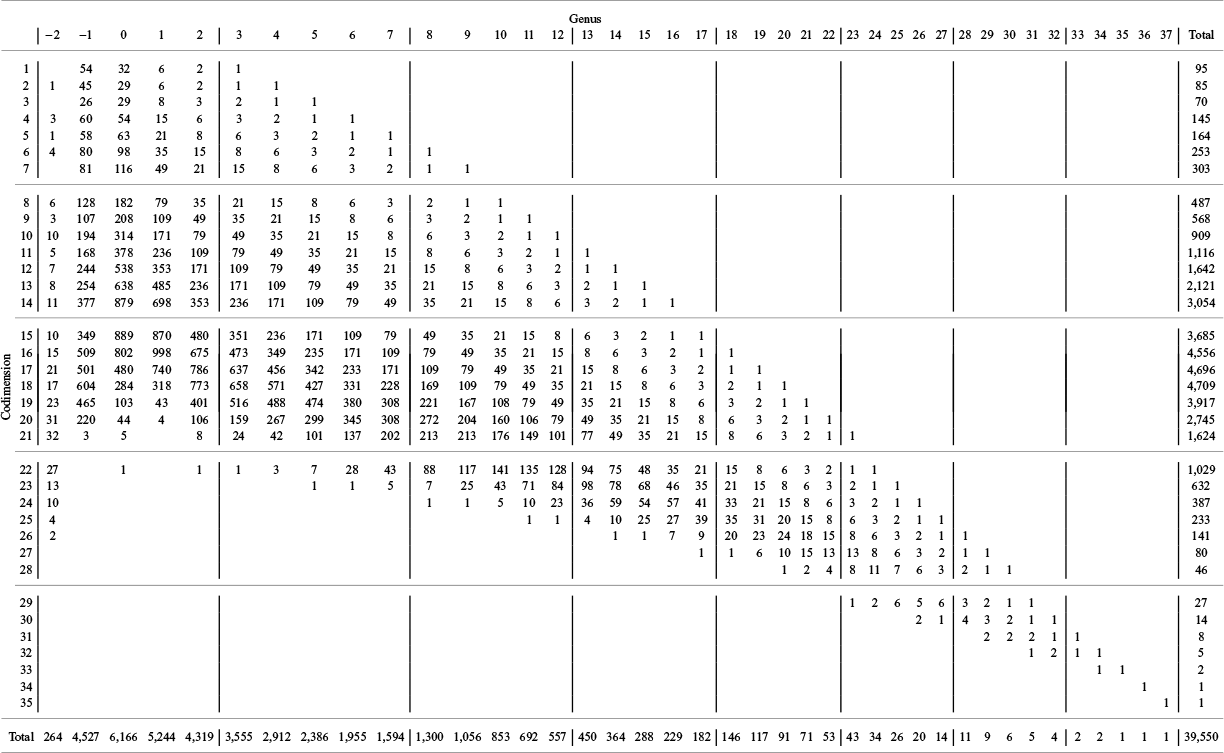


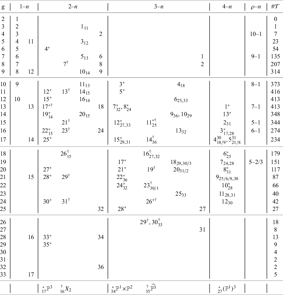


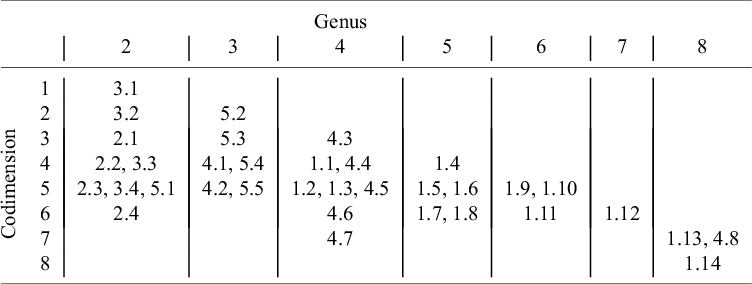


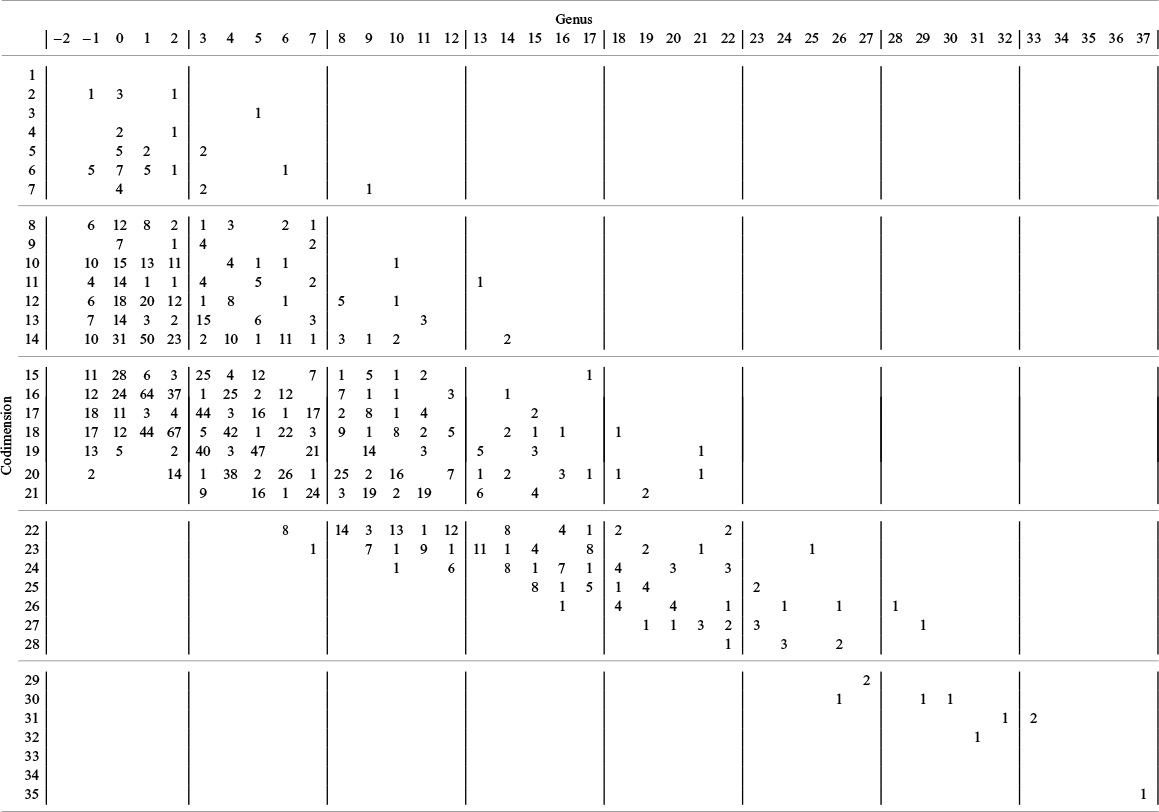


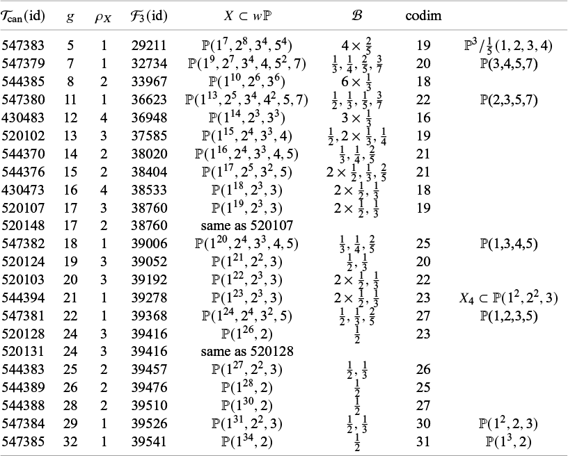


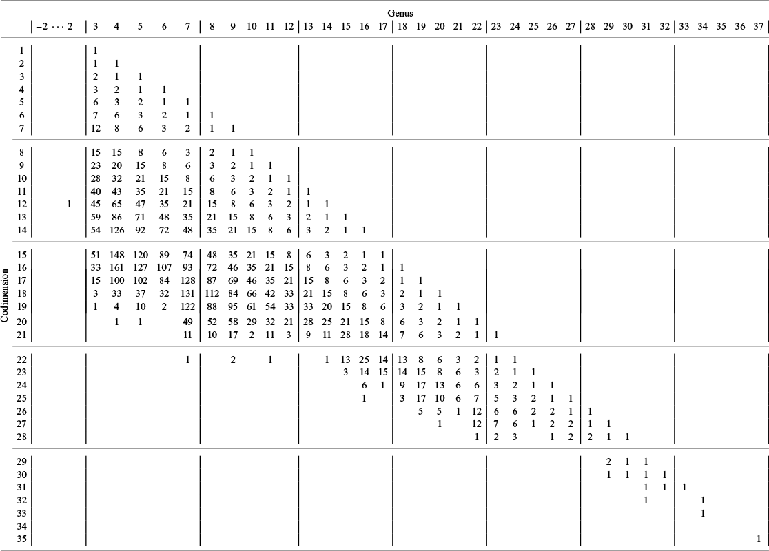


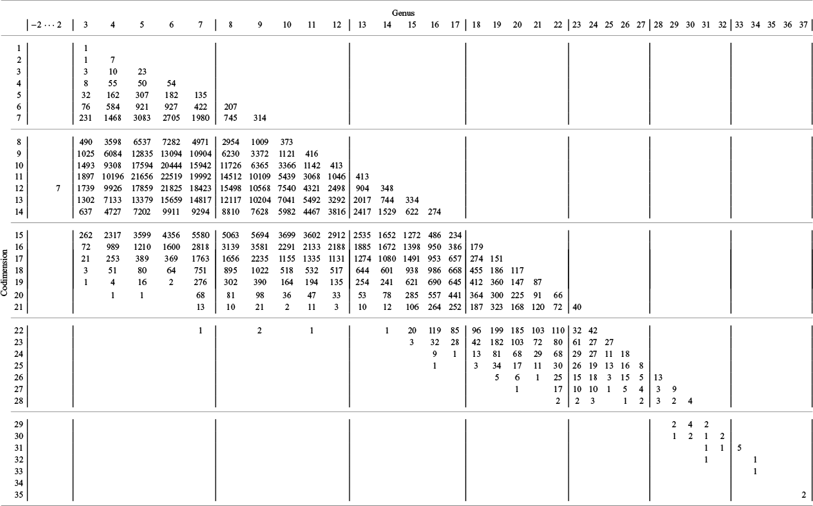


 Open access

