


1. Introduction
Turbulence is traditionally associated with intermittent, stochastic flows. Despite this, in many examples of convective turbulence, the flow is organised into large-scale coherent structures; for example, granulation at the solar surface and cloud streets in the atmosphere (Markson Reference Markson1975; Nordlund, Stein & Asplund Reference Nordlund, Stein and Asplund2009; Pandey, Scheel & Schumacher Reference Pandey, Scheel and Schumacher2018). The most fundamental and ubiquitous coherent structure in thermal convection is the large-scale circulation (LSC) – approximately described as a quasi-two-dimensional overturning motion of the fluid bulk (Krishnamurti & Howard Reference Krishnamurti and Howard1981; Villermaux Reference Villermaux1995; Funfschilling & Ahlers Reference Funfschilling and Ahlers2004; Zhou et al. Reference Zhou, Xi, Zhou, Sun and Xia2009), but also subject to a variety of complex dynamics, as we will discuss further in this work. The LSC is of central importance for convective turbulence theory; it shears the fluid where thermal plumes are ejected from boundary layers into the bulk, and numerous predictions for the transport properties of convective systems rely on this sweeping effect as a theoretical launching point (Grossmann & Lohse Reference Grossmann and Lohse2000; Shishkina et al. Reference Shishkina, Horn, Wagner and Ching2015; Ching et al. Reference Ching, Leung, Zwirner and Shishkina2019).
Progress has been made in characterising the LSC in the reduced system of Rayleigh–Bénard convection. In it, a layer of fluid is confined between two parallel plates while being heated from below and cooled from above. An extensive body of work has examined this flow in water and similar fluids, where the ratio between the viscous diffusivity and thermal diffusivity – characterised by the Prandtl number  $Pr = \nu / \kappa$ – is near or larger than unity. Here,
 $\nu$ is the kinematic viscosity and
 $\kappa$ is the thermal diffusion coefficient.
In this canonical set-up, comprised of an aspect ratio  $\varGamma = D/H = 1$ cylindrical container (where
 $D$ is the vessel diameter and
 $H$ is the height) of fluid with
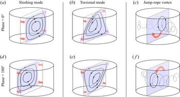
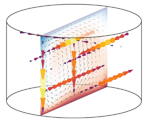
 $Pr \gtrsim 1$, fundamental LSC behaviours have become apparent. Two modes, corresponding to low-frequency oscillations, appear to dominate; a sloshing horizontal translation of the LSC plane and a periodic twisting of the LSC plane around the central axis of the container (Funfschilling & Ahlers Reference Funfschilling and Ahlers2004; Zhou et al. Reference Zhou, Xi, Zhou, Sun and Xia2009; Sun, Xia & Tong Reference Sun, Xia and Tong2005). These so-called ‘sloshing’ and ‘torsional’ modes are illustrated in figure 1(a,b). Although we portray them separately here, it is argued that the two modes are interconnected and inseparable, both arising from the tendency of the LSC to become misaligned with respect to its container (Brown & Ahlers Reference Brown and Ahlers2009; Xi et al. Reference Xi, Zhou, Zhou, Chan and Xia2009).
Periodic motions of the LSC in convection: (a,d) the sloshing mode, (b,e) the torsional mode and (c,f) the jump-rope vortex (JRV) mode. Panels (a–c) correspond to one apex of the motion, set as the initial phase, while panels (d–f) correspond to the opposite phase. The blue region represents the plane of the LSC. Arrows represent motions of the LSC associated with each mode. Dashed lines represent a meridional slice of the vessel, which coincides with the time-averaged plane of the LSC motion in each case.

Convection in liquid metals, for which the thermal diffusivity is orders of magnitude larger than the momentum diffusivity and  $Pr \ll 1$, has received far less attention (Rossby Reference Rossby1969; Takeshita et al. Reference Takeshita, Segawa, Glazier and Sano1996; Cioni, Ciliberto & Sommeria Reference Cioni, Ciliberto and Sommeria1996, Reference Cioni, Ciliberto and Sommeria1997; Glazier et al. Reference Glazier, Segawa, Naert and Sano1999; Aurnou & Olson Reference Aurnou and Olson2001; King, Stellmach & Buffett Reference King, Stellmach and Buffett2013; Frick et al. Reference Frick, Khalilov, Kolesnichenko, Mamykin, Pakholkov, Pavlinov and Rogozhkin2015; Schindler et al. Reference Schindler, Eckert, Zürner, Schumacher and Vogt2022; Xu, Horn & Aurnou Reference Xu, Horn and Aurnou2022). This is despite a broad range of applications; low-
 $Pr$ convection is involved in interiors of terrestrial planets (Aurnou et al. Reference Aurnou, Calkins, Cheng, Julien, King, Nieves, Soderlund and Stellmach2015), turbulent regions of stars (Hanasoge, Gizon & Sreenivasan Reference Hanasoge, Gizon and Sreenivasan2016), industrial processing of materials (Asai Reference Asai2012) and energy technologies such as liquid metal batteries (Kelley & Weier Reference Kelley and Weier2018), among other systems.
In  $Pr \ll 1$ fluids, the thermal boundary layers at the top and bottom boundaries are significantly thicker than the momentum boundary layers, leading to significantly larger thermal plumes detaching from the boundary layers and enhanced vorticity generation (Schumacher, Götzfried & Scheel Reference Schumacher, Götzfried and Scheel2015). The result is distinct dynamics, scaling properties and statistics from
 $Pr \gtrsim 1$ flows (Ahlers, Grossmann & Lohse Reference Ahlers, Grossmann and Lohse2009; Scheel & Schumacher Reference Scheel and Schumacher2016, Reference Scheel and Schumacher2017), as well as different interactions between the LSC and the boundary layers (Schumacher et al. Reference Schumacher, Bandaru, Pandey and Scheel2016). One way these distinctions manifest is in the scaling relationships between global parameters. Momentum transport is parametrised by the Reynolds number
 $Re = UH/\nu$, where
 $U$ is a typical velocity, while the thermal forcing is parametrised by the Rayleigh number
 $Ra = \alpha g \Delta T H^3 / \nu \kappa$, where
 $\alpha$ is the coefficient of thermal expansion,
 $g$ is gravitational acceleration and
 $\Delta T$ is the overall temperature difference. In the
 $Ra$ ranges relevant to most applications, Grossmann & Lohse (G–L) theory predicts that
 $Re$ scales as
 $Ra^{1/2}$ in water but as
 $Ra^{2/5}$ in liquid metals (Grossmann & Lohse Reference Grossmann and Lohse2000), a result that has been corroborated in experiments and simulations (Cioni et al. Reference Cioni, Ciliberto and Sommeria1997; Sun & Xia Reference Sun and Xia2005; Scheel & Schumacher Reference Scheel and Schumacher2017; Zürner et al. Reference Zürner, Schindler, Vogt, Eckert and Schumacher2019; Schindler et al. Reference Schindler, Eckert, Zürner, Schumacher and Vogt2022) and points to dynamical differences in the flows.
The majority of  $Pr \ll 1$ convection studies have adhered to the canonical cylinder of aspect ratio
 $\varGamma = 1$ (Ahlers et al. Reference Ahlers, Grossmann and Lohse2009). In it, the sloshing and torsional modes are dominant, as for moderate
 $Pr$ (Horn, Schmid & Aurnou Reference Horn, Schmid and Aurnou2021). But recent studies focusing on
 $\varGamma > 1$ geometries have demonstrated the emergence of another mode, dubbed the jump-rope vortex (JRV) for its resemblance to the flipping motion of a jump rope (Vogt et al. Reference Vogt, Horn, Grannan and Aurnou2018; Zürner et al. Reference Zürner, Schindler, Vogt, Eckert and Schumacher2019; Akashi et al. Reference Akashi, Yanagisawa, Sakuraba, Schindler, Horn, Vogt and Eckert2022; Horn et al. Reference Horn, Schmid and Aurnou2021). This mode appears at relatively high Reynolds values of
 $Re \gtrsim 10^3$ and likely originates in a turbulent environment (Vogt et al. Reference Vogt, Horn, Grannan and Aurnou2018). We illustrate its behaviour in figure 1(c). The JRV is in fact the dominant mode at cylindrical aspect ratios
 $\sqrt {2} \lesssim \varGamma \lesssim 2$ (Vogt et al. Reference Vogt, Horn, Grannan and Aurnou2018). Using dynamic mode decomposition in direct numerical simulations (DNS), Horn et al. (Reference Horn, Schmid and Aurnou2021) found that the JRV is still present even at an aspect ratio
 $\varGamma = 1$, although it is less dynamically important than the slosh and torsional modes. Using laboratory experiments combined with DNS, Akashi et al. (Reference Akashi, Yanagisawa, Sakuraba, Schindler, Horn, Vogt and Eckert2022) discovered that a network of JRVs dominate the LSC dynamics in a cuboid container of sidewall-length-to-height aspect ratio of 5. These results point to the idea that the properties of the LSC – particularly its geometry and the dynamical importance of different modes – vary greatly over a relatively narrow range of moderately large aspect ratios between 1 and 5.
In this work, we present a suite of convection experiments and complementary simulations in liquid gallium ( $Pr = 0.02$) in order to delineate the scaling properties of the primary flow modes and their sensitivity to the container aspect ratio. We conduct a survey over multiple aspect ratios
 $1.4 \le \varGamma \le 3$ and Rayleigh numbers
 $10^4 \lesssim Ra \lesssim 10^6$. Comparing frequency spectra from our laboratory velocity measurements and flow fields from simulations yields quantitative agreement. Normalising the JRV oscillation frequency with a diffusive time scale based on the overall path length collapses it into the same scaling against
 $Ra$ over multiple aspect ratios. While the JRV serves as the dominant flow mode for
 $1.4 \le \varGamma \le 2$, the flow dynamics nonetheless varies with the aspect ratio. A separate spectral peak appears in the temperature and velocity data more consistently as
 $\varGamma$ approaches
 $1$, and filtering around this peak gives evidence that it corresponds to a torsional motion. For
 $\varGamma = 3$, the JRV signature is no longer detectable. Unlike in JRV-dominated regimes, the large-scale flow appears to consist of two or more circulations in the horizontal dimensions, and is prone to reversals in orientation.
Below, in § 2, we outline our laboratory and numerical methods. In § 3 we present and interpret our main findings: § 3.1 looks at scaling between the global parameters, § 3.2 examines features of the flow morphology and 3.5 focuses on individual spectral peaks and connects them to LSC modes. In § 4 we summarise results and discuss the broader implications of this work.
2. Methods
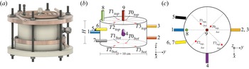
Our study was conducted using a novel laboratory set-up designed and fabricated at the University of Rochester (Cheng et al. Reference Cheng, Wang, Mohammad, Forer and Kelley2021). Figure 2(a) shows the overall layout of the set-up with a design drawing. The working fluid is liquid gallium and is confined in a cylindrical vessel with copper plates for the top and bottom boundaries and an insulating Delrin acetyl polymer cylinder for the sidewall. To explore convection at different aspect ratios, we employ several interchangeable Delrin sidewalls of heights  $H = 3.3, 5.0, 5.9$ and
 $7.1$ cm and inner diameter
 $D = 10$ cm, corresponding to aspect ratios
 $\varGamma = 3, 2, 1.7$ and
 $1.4$.
(a) Design drawing of the experimental set-up. The cylindrical vessel is composed of copper top and bottom plates and a Delrin acetyl polymer sidewall. (b,c) Velocity and temperature measurement probe placements around the set-up. There are nine ultrasound transducers (numbered 1–9 and colour coded) and two sets of four thermocouple probes embedded on both the top and bottom plates (numbered T0–T3 with positions marked by red circles). Horizontal ultrasound probes are placed at heights  $z = H/4$,
 $H/2$ and
 $3H/4$ for
 $\varGamma = 1.4$, 1.7 and 2, and
 $z=H/3$,
 $H/2$ and
 $2H/3$ for
 $\varGamma = 3$. Chord probes 5, 6 and 7 have beams parallel to probe 1 but offset horizontally by
 $D/4$ (the probes are placed at a small angle in order to account for refraction of the beam at the Delrin–gallium interface). Some probes in the
 $\varGamma =3$ vessel are rotated to different locations to conserve space, but they retain radial/chord orientations. Vertical ultrasound probe 9 is located at the radial centre while probe 8 is 4 mm from the sidewall. The radial distances of the thermocouple probes from the central axis are 1.15 cm, 2.30 cm, 3.80 cm and 4.45 cm.

The K-type thermocouple temperature probes are embedded in the top and bottom plates, within 3 mm of the fluid layer, as shown in figure 2(b,c). Signals are recorded by a set of National Instruments NI 9211 cDAQ modules and read into LabVIEW. We induce convection in the gallium layer using heat exchangers attached to each copper plate. Water is pumped through the heat exchangers from a pair of thermal baths; a VWR 1136 heated circulating water bath for the bottom plate and a Thermo Neslab RTE7 chiller for the top plate. The heat exchangers consist of non-inductively wound copper tubing, ensuring uniform temperatures across plates to  ${<}5\,\%$ of the vertical temperature difference for almost all cases. Thermocouple measurements serve as a diagnostic tool, and they are also useful for controlling the device; the heat exchangers are tuned such that the mean temperature
 $(\overline {T}_{bot} + \overline {T}_{top})/2$ always remains in the neighbourhood of
 $43\,^\circ {\rm C}$ and the fluid properties of the gallium remain nearly constant over all cases (see table 2 in the Appendix). Here, the overline indicates spatial averaging across all top or bottom temperature probes. On average, the viscous diffusivity
 $\nu = 2.6 \times 10^{-7}\,\mathrm {m}^2\,\mathrm {s}^{-1}$, thermal diffusivity
 $\kappa = 1.3 \times 10^{-5}\,\mathrm {m}^2\,\mathrm {s}^{-1}$ and coefficient of thermal expansion
 $\alpha = 1.3 \times 10^{-4}\,\mathrm {K}^{-1}$. The fluid properties are estimates based on published values (Davidson Reference Davidson1968; Okada & Ozoe Reference Okada and Ozoe1992; Prokhorenko et al. Reference Prokhorenko, Roshchupkin, Pokrasin, Prokhorenko and Kotov2000; Iida & Guthrie Reference Iida and Guthrie2015a,Reference Iida and Guthrieb). Further details on the set-up, probe layout and gallium properties can be found in Cheng et al. (Reference Cheng, Wang, Mohammad, Forer and Kelley2021).
Our other primary diagnostic tool is an array of ultrasound probes placed around the vessel in various positions and angles, again shown in figure 2(b,c). Using ultrasonic Doppler velocimetry (UDV), these probes give us one-component velocity profiles along each probe beam. Much of the following analysis will make use of these velocity measurements and their statistics.
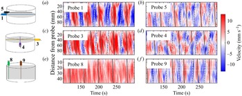
Figure 3 shows typical measurements from six of the ultrasound probes. These high-resolution Dopplergrams – one-dimensional velocities plotted as colour, varying over a distance and time – reveal a strong periodic signal which we will argue is associated with the JRV. We can estimate typical velocities in the flow using the free-fall velocity  $U_{ff}$, the characteristic velocity associated with the leading-order balance between inertial and buoyancy terms
 \begin{equation} U_{ff} = \left(\alpha g \Delta T H \right)^{1/2} , \end{equation}
where  $\Delta T = \langle \overline {T}_{bot} - \overline {T}_{top} \rangle$ and ‘
 $\langle \,{\cdot }\, \rangle$’ signifies an average over time. Assuming a single flow structure, the path length of the LSC is coarsely approximated by
 $L = 2H + 2D$ (Vogt et al. Reference Vogt, Horn, Grannan and Aurnou2018), and an associated free-fall circulation time
 $\tau _{ff} = L/U_{ff}$ and free-fall circulation frequency
 $f_{ff} = 1/\tau _{ff}$ can be derived as useful quantities for our subsequent discussion. Since the Dopplergrams in figure 3 show distance vs time, we can represent
 $U_{ff}$ as diagonal lines in each panel. Compared with the angle of streaks in the Dopplergrams, we see that
 $U_{ff}$ qualitatively serves as a slight overestimate for the speed of LSC motion.
Dopplergrams showing velocity as a function of distance from probe and time, from a convection case at  $Ra = 6.5 \times 10^5$ (
 $\Delta T=8.8\,^\circ$C,
 $\varGamma = 1.7$). All of the probes used for a typical case are included here, with numbers and positions given in figure 2. Features with slopes matching the solid or dotted lines move away from or toward the probe, respectively, with speed equal to the free-fall speed
 $U_{ff}$.

We compare our experimental results with complementary DNS. The DNS were performed using the open-source finite volume solver OpenFOAM. The discretisation scheme utilised a fourth-order cubic interpolation scheme in space and a fourth-order least-squares scheme to calculate the surface normal gradients. The second-order accurate implicit Euler scheme was used for time advancement. The incompressible Navier–Stokes equations were solved using the Oberbeck–Boussinesq approximation. The conservation of momentum is given by
 \begin{equation} \frac{\partial \boldsymbol{u}}{\partial t}+\left(\boldsymbol{u} \boldsymbol{\cdot} \boldsymbol{\nabla} \right)\boldsymbol{u} - \nu \nabla^2 \boldsymbol{u} = \frac{1}{\rho_0}\boldsymbol{\nabla}\left(\rho_0 \boldsymbol{g}z - p\right) -\boldsymbol{g}\alpha(T-T_0) , \end{equation}
in which  $t$ is time,
 $\boldsymbol {u}$ is the velocity vector,
 $\rho _0$ is the density,
 $\boldsymbol {g}$ is the gravitational acceleration vector,
 $z$ is the vertical depth,
 $p$ is the pressure and
 $T$ is the temperature. The continuity equation is
 \begin{equation} \boldsymbol{\nabla} \boldsymbol{\cdot} \boldsymbol{u} = 0 , \end{equation}
and finally, the temperature is calculated using the energy equation
 \begin{equation} \frac{\partial T}{\partial t} + \boldsymbol{u}\boldsymbol{\cdot} \boldsymbol{\nabla} T = \frac{k}{\rho_0 C_p}\nabla^2T, \end{equation}
in which  $k$ is the thermal conductivity and
 $C_p$ is the heat capacity. Dirichlet boundary conditions for temperature were used on the top and bottom boundaries, while the sidewalls were considered to be perfectly insulating due to the low thermal conductivity of the Delrin. No-slip boundary conditions were used on all surfaces to solve the equation for the conservation of momentum. The main DNS was carried out on the study with
 $\varGamma = 1.4$ and
 $Ra = 1.2 \times 10^{6}$, with grid dimensions of
 $N_x \times N_y \times N_z=222 \times 222 \times 158$. The computations were carried out for a duration of
 $500 \tau _{ff}$ after a statistically steady state was reached. Mesh convergence was checked by comparing the Nusselt number at the top boundary against a finer grid with a resolution of
 $N_x \times N_y \times N_z=296 \times 296 \times 211$. The Nusselt number was found using
 \begin{equation} Nu= \frac{hl}{k} , \end{equation}
in which  $h$ is the heat transfer coefficient and
 $l$ is the characteristic length which, in this case, we define as the height of the domain. The heat transfer coefficient was calculated using
 \begin{equation} h= \frac{q}{\Delta T} , \end{equation}
in which  $q$ is the heat flux at the top boundary and
 $\Delta T = T_H-T_C$. An average was computed for six times the turnover time resulting in a value of
 $Nu = 4.14$ and 4.15 for the coarse and fine grid, respectively. With only a 0.24 % difference found between the two grid sizes, we considered the mesh converged.
3. Results
3.1. Global parameters
Global parameters provide a broad indication of the underlying dynamics in the system. In convective systems, the Reynolds number and the Rayleigh number are known to follow a power law scaling of the form  $Re = c_{Re}Ra^{\gamma _{Re}}$, where
 $c_{Re}$ and
 $\gamma _{Re}$ are constants. We plot
 $Re$ vs
 $Ra$ values in figure 4. An added complication arises from the fact that many methods exist for estimating
 $Re$ based on velocities. Previous studies have shown that even measurements from a single ultrasound probe can produce
 $Re$ values that scale as predicted theoretically (Vogt et al. Reference Vogt, Horn, Grannan and Aurnou2018; Zürner et al. Reference Zürner, Schindler, Vogt, Eckert and Schumacher2019), despite only giving one component of the velocity vector along one line. We estimate
 $Re$ using three different methods:
(i) We take the time and space root-mean-square (r.m.s.) of velocities measured by probe 1, which is oriented radially through the tank at height
 $H/2$. We refer to this speed estimate as $U_{r}$.
(ii) Beams from probes 3, 4 and 9 all intersect at a single point at the central axis of the tank, forming an orthogonal basis for the velocity vector at that point, which we name
$P$. Assuming a Cartesian coordinate system with the origin at the bottom of the central axis of the vessel, point $P$ has coordinates $(x,y,z) = (0,0,3H/4)$ in the $\varGamma = 1.4$, $\varGamma = 1.7$ and $\varGamma = 2$ vessels. In the $\varGamma = 3$ vessel, in which spatial constraints require different probe placements, the coordinates of $P$ are $(0,0,2H/3)$. The speed at $P$ is
(3.1)where\begin{equation} U_{3D} = \sqrt{ \left\langle u^2_x\left(P\right) + u^2_y\left(P\right) + u^2_z\left(P\right) \right\rangle } , \end{equation}$u_x$, $u_y$ and $u_z$ are measured by probes 4, 3 and 9, respectively. To reduce noise, we include velocity measurements in the vicinity of $P$; if $\ell$ represents the total length of a given probe beam, we take the spatial r.m.s. of measurements within $\ell /8$ of $P$ for each probe.(iii) From figure 3, there appears to be a single spatial structure detected by probe 3. For this estimate, we therefore assume that the vessel is populated by a single LSC. The intersection of probes 3 and 4 at
$P$ is near the top of the tank, so we use them to estimate the overturning velocity of the LSC (which is approximately horizontal there)
(3.2)This estimate closely follows the methodology of Zürner et al. (Reference Zürner, Schindler, Vogt, Eckert and Schumacher2019), but without averaging against another position near the bottom of the tank since we only have one radial probe at\begin{equation} U_{LSC} = \sqrt{ \left\langle u^2_x\left(P\right) + u^2_y\left(P\right) \right\rangle } . \end{equation}$z = H/4$.


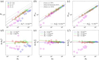
Variation of the Reynolds number  $Re$ with the Rayleigh number
 $Ra$ for all convection cases. Simulation cases are plotted as yellow hexagrams. Best-fit scaling trends over all aspect ratios are plotted as black lines. Also plotted for comparison are the best-fit scaling slopes from previous low-
 $Pr$ convection studies:
 $Re = 12 Ra^{0.424}$ (Cioni et al. Reference Cioni, Ciliberto and Sommeria1997),
 $Re = 6.5 Ra^{0.45}$ (Scheel & Schumacher Reference Scheel and Schumacher2017) and
 $Re = 8.0 Ra^{0.42}$ (Zürner et al. Reference Zürner, Schindler, Vogt, Eckert and Schumacher2019). Panels (a–c) show
 $Re$ vs
 $Ra$ using estimates of
 $Re$ based on
 $U_r$,
 $U_{3D}$ and
 $U_{LSC}$, respectively. Panels (d–f) show
 $Re$ compensated by the overall best-fit scaling trends vs
 $Ra$, with coloured lines representing the best-fit trends for individual aspect ratios. Yellow hexagrams represent velocity measurements from the simulation case.

Figure 4 shows the scaling properties of  $Re$ with
 $Ra$ following our above estimates for the typical velocity, where
 $Re_{r}=U_{r}H/\nu$,
 $Re_{3D}=U_{3D}H/\nu$,
 $Re_{LSC}=U_{LSC}H/\nu$ and
 $H$ varies with the aspect ratio as described in § 2. Figure 4(a) shows that
 $U_r$ produces a seemingly robust scaling of
 $Re_r = 3.9^{+1.5}_{-1.1} Ra^{0.46 \pm 0.03}$, near the G–L theory prediction and previous studies at
 $\varGamma = 1.7$ and 2, although it underestimates the prefactor by approximately a factor of 2. (The uncertainties represent 95 % confidence intervals in a linear polynomial fit to the logarithm of the scaling. Subsequent best-fit scaling arguments use the same fitting method.) Results are in close agreement with Zürner et al. (Reference Zürner, Schindler, Vogt, Eckert and Schumacher2019), who found
 $Re = 3.1 Ra^{0.46}$ for a similar probe position. The
 $Re$ values are generally smaller than other published predictions, as expected in the mid-height region where horizontal velocities tend to be weak (Qiu & Tong Reference Qiu and Tong2001; Ahlers et al. Reference Ahlers, Grossmann and Lohse2009). However, data do not appear to collapse meaningfully for the
 $\varGamma = 1.4$ or 3 geometries. One explanation for this is related to the fact that an LSC by nature produces slow horizontal velocities at the mid-height horizontal plane; the largest component of LSC flow in this region is vertical (Qiu & Tong Reference Qiu and Tong2001). If the JRV mode is most energetic at
 $\varGamma \approx 2$, its vigorous orbital motion could periodically lift the core of the LSC outside of the mid-height plane (see figure 1), allowing horizontal flow outside the core region to sweep in and be detected by probe 1. This would increase the average velocity. On the other hand, when the JRV motion is weaker, we speculate that this effect is dampened and average velocities lowered. If we use this model to explain the lower
 $U_r$ velocities when
 $\varGamma = 1.4$ and
 $\varGamma = 3$, it is consistent with the prevalence of other modes unique to these geometries, which we discuss further in § 3.4.
Figure 4(b,c) demonstrates that  $Re_{3D}$ and
 $Re_{LSC}$ are both successful at collapsing data to a single best-fit scaling across
 $1.4 \le \varGamma \le 2$;
 $Re_{3D} = 8.4^{+2.3}_{-1.8} Ra^{0.43 \pm 0.02}$ in the former case and
 $Re_{LSC} = 10.8^{+1.5}_{-1.3} Ra^{0.41 \pm 0.01}$ in the latter. For
 $Re_{3D}$, data points from
 $\varGamma = 3$ other than the two clear outliers at the lowest
 $Ra$ values are included in the fit, while for
 $Re_{LSC}$, the fit only includes
 $1.4 \le \varGamma \le 2$. The case of
 $Re_{3D}$ collapses most of the data points from
 $\varGamma = 3$, but
 $Re_{LSC}$ does not, likely because the flow at
 $\varGamma = 3$ is no longer dominated by a single, horizontal LSC, running counter to the assumption underlying (3.2). We will expand on this when examining the flow morphologies in § 3.2. Curiously, however,
 $Re_{LSC}$ does a better job of collapsing
 $1.4 \le \varGamma \le 2$ data. Ultimately, both methods are in line with the results of Zürner et al. (Reference Zürner, Schindler, Vogt, Eckert and Schumacher2019) who found a best-fit relation of
 $Re = 8.0 Ra^{0.42}$. The absolute
 $Re$ values for all methods give
 $Re = O(10^3)$, in line with parameter ranges where the JRV has been observed (Vogt et al. Reference Vogt, Horn, Grannan and Aurnou2018; Akashi et al. Reference Akashi, Yanagisawa, Sakuraba, Schindler, Horn, Vogt and Eckert2022).
The DNS measurements for  $Re_{3D}$ and
 $Re_{LSC}$ are also shown in figure 4(b,c). To optimise experimental comparison, we sampled DNS velocities on grid points analogous to the locations sampled by experimental UDV probes; we defined ‘virtual probes’ oriented similarly to probes 3 and 4 with respect to the LSC, selected grid points that lay in the probe beams’ diameters (approximated as 5 mm) and within
 $\ell /8$ of
 $P$ and obtained a spatial r.m.s. of the velocity components axial to each probe at these grid points. Both the two- and three-dimensional measurements show good agreement with experimental data;
 $Re_{LSC|{DNS}} = 3228$ and
 $Re_{3D|{DNS}} = 3648$ lying 1.0 % and 6.1 %, respectively, above corresponding experimental values at
 $\varGamma = 1.4$,
 $Ra = 1.18\times 10^6$ (see table 2 in the Appendix). A possible source of mismatch could be systematic error in our
 $Ra$ estimates; the material properties of gallium have seen a broad range of measured values, with
 $\nu$ differing by as much as 40 % for a given temperature (Brandes & Brook Reference Brandes and Brook1992; Okada & Ozoe Reference Okada and Ozoe1992; Iida, Guthrie & Tripathi Reference Iida, Guthrie and Tripathi2006; Xu et al. Reference Xu, Oudalov, Guo, Jaeger and Brown2012; Aurnou et al. Reference Aurnou, Bertin, Grannan, Horn and Vogt2018). We employ some of the most recent estimates, as discussed in Cheng et al. (Reference Cheng, Wang, Mohammad, Forer and Kelley2021). Mismatches between our assumed material properties and reality would cause a translation of our results to different
 $Ra$ and
 $Re$ numbers, changing the prefactors of the scaling relationships shown in figure 4 but not affecting the exponents.
Figure 4(d–f) shows the same data, compensated by the overall best-fit scaling trend for each  $Re$ estimate. Within these plots, the scaling trends for data at each
 $\varGamma$ are plotted as coloured lines. Differences between the best-fit scaling exponents are small but not insignificant. This may be because, while the probe beams are fixed at
 $z = 3H/4$, the position of the JRV vortex core relative to the probe beams varies with
 $Ra$. The nature of this variation likely changes with the JRV confinement, determined by
 $\varGamma$. A speculative explanation is that the faster JRV overturn cycle at higher
 $Ra$ could lead to a different amplitude of the orbital motion, such that each subsequent case at higher
 $Ra$ presents a different region of the flow to the probes at
 $P$.
Although one might expect the JRV to complicate velocity estimates compared with a more stationary LSC in, say,  $\varGamma = 1$ containers, our results are ultimately consistent with the predictions of G–L theory and previous DNS and experiments.
3.2. Flow morphology
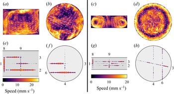
In figure 5, we compare the typical flow morphologies at  $\varGamma = 1.4$ and
 $\varGamma = 3$. Cross-sections of the velocity field from the simulations are compared with experimental measurements. Although only one component of the velocity vector appears for each probe, the structure of the fields and velocity magnitudes appear to agree. Between
 $\varGamma = 1.4$ and 3, an immediate contrast is clear; while a single LSC dominates the
 $\varGamma = 1.4$ dynamics (see also supplementary movie 1 available at https://doi.org/10.1017/jfm.2022.778), a torus-like LSC is present for
 $\varGamma = 3$, giving two overturning structures and an intermittent central region for any meridional slice of the flow. The roughly axisymmetric morphology in
 $\varGamma = 3$ DNS is not fully consistent with experimental observations – for example, on a given horizontal plane, flows converging toward the central axis in the
 $x$-direction often occur in concert with diverging flows in the
 $y$-direction (roughly observed in figure 5h). Further analysis at this aspect ratio will concern experimental data. Like the DNS, a single LSC-style structure is certainly not dominant in any
 $\varGamma = 3$ experiment.
Visualisations of the flow in simulations (a–d) compared with velocity measurements in experiments (e–h). Panels (a,b,e,f) show  $\varGamma = 1.4$ data at
 $Ra=1.2\times 10^6$ while panels (c,d,g,h) show
 $\varGamma = 3$ data at
 $Ra= 1.4\times 10^5$. Panels (a,c,e,g) show vertical slices of the flow. Panels (b,f) show horizontal slices at height
 $3H/4$. Panels (d,h) show horizontal slices at height
 $2H/3$. The overall flow morphology visible in simulations is also captured by experimental UDV measurements.

A feature unique to  $\varGamma = 3$, and present in both DNS and experiments, is the occurrence of reversals in the flow direction. This LSC behaviour is known to occur at many Prandtl numbers and vessel geometries (Yanagisawa, Hamano & Sakuraba Reference Yanagisawa, Hamano and Sakuraba2015; Schumacher et al. Reference Schumacher, Bandaru, Pandey and Scheel2016; Tasaka et al. Reference Tasaka, Igaki, Yanagisawa, Vogt, Zuerner and Eckert2016; Akashi et al. Reference Akashi, Yanagisawa, Tasaka, Vogt, Murai and Eckert2019). In wider aspect ratios, it can be interpreted as an effect of the confinement, where transitions between different numbers of rolls cause reorientations of the whole flow field (Yanagisawa et al. Reference Yanagisawa, Hamano and Sakuraba2015; Tasaka et al. Reference Tasaka, Igaki, Yanagisawa, Vogt, Zuerner and Eckert2016; Akashi et al. Reference Akashi, Yanagisawa, Tasaka, Vogt, Murai and Eckert2019). Small-scale turbulence can also be responsible for reversals even in
 $\varGamma = 1$ systems, triggering extreme dissipation events that disrupt the LSC (Schumacher & Scheel Reference Schumacher and Scheel2016). In our set-up, reversals seem to occur with some regularity, happening during several one hour experiments. We therefore believe the more likely culprit is confinement of the LSC rolls rather than rare dissipation events. Further support for this view comes from observations that the flow at the sidewall probe 8 is occasionally oriented downward, despite usually being oriented upward; one example is our
 $Ra = 7.7 \times 10^4$ case. The fact that cases at both higher and lower
 $Ra$ values return to a downward flow at the sidewall may reflect a somewhat arbitrary orientation of the rolls depending on the initial conditions. In a similar fashion, a simulation at
 $Ra = 1.38 \times 10^5$ has given upward rolls at the sidewalls while, at only a small increase in the
 $Ra$, the flow re-orients, with a simulation at
 $Ra = 1.62 \times 10^5$ giving downward rolls on the sidewall.
Although not shown in figure 5, the flow morphologies at  $1.7 \le \varGamma \le 2$ bear strong resemblance to those at
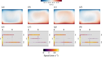
 $\varGamma = 1.4$. The flow is oscillatory nearly everywhere, such that its morphology depends heavily on the cycle of the JRV. The exception to this is probe 8, which closely tracks the sidewall of the vessel and therefore lies outside of the JRV orbit, detecting its signal only weakly. Figure 6 demonstrates that conditionally averaging both simulations and experiments with respect to the JRV oscillation frequency clearly reveals a flipping jump-rope motion. The vortex core, marked by a region of low flow speed, starts on the right central side of the LSC plane. We associate this with a phase of
 $0^\circ$. It then migrates to the central lower region of the plane at a phase of
 $90^\circ$ and continues a clockwise, roughly circular motion until returning to the initial position. Note that while the JRV migration is clockwise, the LSC flow is counterclockwise. Our observations are consistent with the thorough analysis of JRV motion in Vogt et al. (Reference Vogt, Horn, Grannan and Aurnou2018). Supplementary movies 2a and 2b show videos of the conditionally averaged flow in simulations and experiments, respectively.
Conditionally averaged snapshots of the flow field at different points in the JRV cycle at  $Ra = 1.2 \times 10^{6}$,
 $\varGamma = 1.4$. (a–d) Vertical slices of the simulated velocity field (arrows) and temperature field (background colour). (e–h) Velocity components measured in experiments. From left to right, the panels correspond to phases 0
 $^\circ$, 90
 $^\circ$, 180
 $^\circ$ and 270
 $^\circ$ of the JRV cycle. At phase 0
 $^\circ$, the vortex core is near mid-height on the right-hand side. Over the cycle, it orbits along a circular path in the clockwise sense, opposite the counterclockwise circulation of the LSC.

3.3. Spectral information
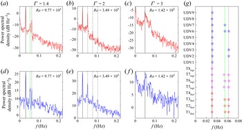
Thus far, we have discussed the overarching flow morphology in which a single mode appears dominant. In truth, however, a variety of modes are expected to occur (Horn et al. Reference Horn, Schmid and Aurnou2021). As these modes are periodic in nature, we build insight into them with spectral analysis. In figure 7, we compare the power spectral density, calculated via Welch's method, of individual temperature and velocity probe measurements across all aspect ratios. For  $1.4 \le \varGamma \le 2$ a prominent peak at lower frequencies corresponds to the JRV motion described above and in figure 6. Other peaks at integer multiples of this frequency are the harmonics of the JRV motion. The harmonic signal in our experiments is consistently stronger than in previous studies (Vogt et al. Reference Vogt, Horn, Grannan and Aurnou2018; Horn et al. Reference Horn, Schmid and Aurnou2021), and furthermore does not manifest as clearly in the DNS.
Power spectral density of (a–c) temperature measurements from thermocouple TC2 $_{bot}$ and (d–f) spatially averaged velocity measurements from velocity probe 6, with aspect ratio and Rayleigh number varying as shown. Solid black lines mark the lowest clear frequency and dashed black lines appear where a harmonic peak was identified. Green lines mark another spectral peak that is most prominent at lower
 $\varGamma$. (g) Frequencies of spectral peaks measured in all temperature and velocity probes from the
 $\varGamma = 1.4$ case shown in (a,d).

At  $\varGamma = 3$, we rarely observe a spectral peak at the expected JRV frequency, and often no peak is present in the typical measurements shown in figure 7(c) or 7(f). Instead, broader peaks consistently manifest at higher frequencies. At low
 $\varGamma$, a recurring feature appears across most
 $Ra$ values; a peak close to the harmonic peak but distinct enough to count separately. We mark this peak with a green line. Thermocouple probes and UDV probes produce spectral peaks in close agreement with each other.
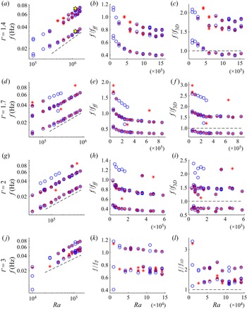
Figure 8 shows the frequencies of selected peaks in experiments at varying values of  $Ra$ and
 $\varGamma$. Examining the full ensemble of cases in the first column, we see that these frequency peaks line up along several power-law scaling trends. For each
 $\varGamma$, peak frequencies appear to be well characterised by
 $Ra^{0.4}$ variation at high
 $Ra$; this result is consistent with prior studies (Cioni et al. Reference Cioni, Ciliberto and Sommeria1997; Ahlers et al. Reference Ahlers, Grossmann and Lohse2009; Vogt et al. Reference Vogt, Horn, Grannan and Aurnou2018; Zürner et al. Reference Zürner, Schindler, Vogt, Eckert and Schumacher2019). However, the frequencies deviate from this trend at lower
 $Ra$ values. We will expand on this discussion of frequency scaling in § 3.5.
Peak frequencies varying with  $Ra$ for each probe in each case. Red stars represent peaks in the temperature spectra while blue circles represent peaks in the velocity spectra. Simulation data are plotted as yellow hexagrams. Panels (a–c), (d–f), (g–i) and (j–l) show data from
 $\varGamma = 1.4$, 1.7, 2 and 3, respectively. Panels (a,d,g,j) contain raw frequencies, and the dashed lines in each panel represent
 $f \sim Ra^{0.4}$. Panels (b,e,h,k) show peak frequencies normalised by the free-fall frequency,
 $f_{ff}$. Panels (c,f,i,l) show peak frequencies normalised by the turnover frequency derived from velocity measurements,
 $f_{3D}$. A dashed black line is plotted at
 $f/f_{3D}=1$. We associate the lowest-frequency peaks at each
 $Ra$ with the JRV, except for
 $\varGamma =3$, where the flow morphology is less clear. For
 $\varGamma =1.7$ and 2, higher-frequency peaks are harmonics of the main peak. At
 $\varGamma = 1.4$, an additional set of peaks occurs at slightly lower frequency than this harmonic. At
 $\varGamma = 3$, the secondary set of peaks does not appear to be a harmonic of the lowest-frequency signal.

In the second column of figure 8, the frequencies are normalised by the free-fall frequency  $f_{ff}$. At high
 $Ra$ we observe that the scaling trend approaches a flat slope at each aspect ratio, indicating that the frequencies become directly proportional to the turnover time, as expected for LSC modes (and thus that
 $f_{ff} \propto Ra^{1/2}$). The region of transient
 $f/f_{ff}$ increases as
 $\varGamma \rightarrow 1$. Several different explanations could be employed for this behaviour; at low
 $\Delta T$, the temperature control may not be robust enough to prevent horizontal gradients across the boundaries which could accelerate existing flow modes. The flow may be in a transient state where the canonical modes are interacting with other chaotic motions. Notably,
 $\varGamma = 1.4$ data take the longest to settle to a constant scaling; this may reflect the weaker nature of the JRV mode for
 $\varGamma = 1.4$. Finally, it may be the case that flow is too near convective onset, where power-law scalings do not manifest consistently (Chandrasekhar Reference Chandrasekhar1961; Rossby Reference Rossby1969); however, our
 $Re$ vs
 $Ra$ trends appear robust in this region. To be safe, the remaining analysis in this work focuses on higher
 $Ra$ ranges where
 $f/f_{ff}$ has settled toward a constant value.
In the third column of figure 8, the frequencies are normalised by  $f_{3D} = L/U_{3D}$. This is a turnover frequency based on
 $U_{3D}$, the velocity estimate that most successfully collapses
 $Re$ vs
 $Ra$ trends across all aspect ratios. The peak frequencies again approach a constant value with increasing
 $Ra$, but apparently more quickly. For most cases, the frequency of the lowest peak resides near
 $f_{3D}$, indicating that flow occupies the whole vessel and that
 $L$ provides a reasonable estimate for the path length of the primary mode. Higher
 $f/f_{3D}$ values for the peaks in
 $\varGamma = 3$ indicate that motions generally take place on a shorter path length than
 $L$, consistent with the multiple rolls observed in figure 5.
A DNS frequency peak from  $z = 3H/4$ temperature measurements is included in figure 8(a). It is in excellent agreement with laboratory measurements:
 $f_0 = 3.39 \times 10^{-2}$ for the lowest-frequency peak in the experimental case and
 $f_0 = 3.51 \times 10^{-2}$ in the DNS.
3.4. LSC dynamics
The orientation angle of the LSC provides a useful launching point for our discussion of the dynamics. Many prior studies have made use of temperature measurements around the sidewall of the container at a fixed height to determine the orientation of the LSC (Cioni et al. Reference Cioni, Ciliberto and Sommeria1997; Zhou et al. Reference Zhou, Xi, Zhou, Sun and Xia2009; Vogt et al. Reference Vogt, Horn, Grannan and Aurnou2018; Zürner et al. Reference Zürner, Schindler, Vogt, Eckert and Schumacher2019). In our set-up, we are limited to eight thermocouple probes which we rely on for accurate measurements of  $\Delta T$ between the top and bottom boundaries.
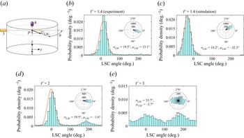
We instead estimate the angle of the LSC with velocity measurements, again making use of the intersection between probes 3 and 4 at  $P$ in a similar fashion to Zürner et al. (Reference Zürner, Schindler, Vogt, Eckert and Schumacher2019). Figure 9(a) shows a schematic of this technique. For
 $1.4 \le \varGamma \le 2$, where a single LSC roll dominates, the direction of the flow at
 $P$ is determined by the LSC orientation. We use the spatial mean of the central 25 % of each probe beam in order to account for noise. Figure 9(b) shows a histogram of the orientation of the LSC at
 $\varGamma = 1.4$,
 $Ra = 1.2 \times 10^6$. We see that the average orientation of the LSC (which we call
 $\mu _{LSC}$) appears to be generally fixed close to the
 $y$-direction, with a standard deviation (
 $\sigma _{LSC}$) in the angle of only 19.5
 $^{\circ }$. In figure 9(c), we conduct the same analysis for the simulation case at
 $\varGamma = 1.4$ and
 $Ra = 1.2 \times 10^6$ using the virtual velocity probes described in § 3.1. This method gives
 $\sigma _{LSC} = 18.2$, seemingly in close agreement with experiments.
Orientation of the LSC estimated from velocity measurements. (a) Schematic showing our methods for estimating orientation. Other panels show distributions of the orientation  $\theta$ over one hour each at (b)
 $\varGamma = 1.4$ and
 $Ra = 1.2 \times 10^6$, (d)
 $\varGamma = 2$ and
 $Ra = 4.7 \times 10^5$ and (e)
 $\varGamma = 3$ and
 $Ra = 1.4 \times 10^5$. Panel (c) shows the same analysis applied to the DNS case (same parameters as panel b). Curves in panels (b–d) indicate normal distribution fits omitting the noisy regions where
 $\|\theta - \mu \| > 70^\circ$ (
 $100^\circ$ for the simulation in panel c). Here,
 $\mu _{LSC}$ and
 $\sigma _{LSC}$ are the average and standard deviation of the LSC orientation, respectively. The insets show polar histograms, with the radial extent representing the number of counts in each bin.

Much like earlier works, our experiments show motion of the LSC plane around a preferred orientation (Brown & Ahlers Reference Brown and Ahlers2006; Xi, Zhou & Xia Reference Xi, Zhou and Xia2006). Unlike those works, however, our experiment manifests the same preferred orientation for each experimental run. We posit that our observed preference is likely due to small inhomogeneities in the boundaries of the gallium layer, where perturbations on the top plate from the filling and overflow ports could become preferential locations for plume detachment. Separately from the short time scale modes we observe, the LSC is known to meander on longer time scales of  $O(10^3) \tau _{ff}$, as well as undergo rare cessations and reversals (Tsuji et al. Reference Tsuji, Mizuno, Mashiko and Sano2005; Brown & Ahlers Reference Brown and Ahlers2006; Xi et al. Reference Xi, Zhou and Xia2006; Xie, Wei & Xia Reference Xie, Wei and Xia2013). We do not observe these behaviours, likely due to a combination of one hour-long runs, strong momentum diffusion in liquid metal and relatively low
 $Ra$ numbers compared with those works.
Figure 9(d) shows that, at  $\varGamma = 2$, a normal distribution again seems to describe the majority of LSC orientations. However, in contrast to the
 $\varGamma = 1.4$ data, orientations near 180
 $^\circ$ also appear at most
 $Ra$ values. Angles in between 0
 $^\circ$ and 180
 $^\circ$ are largely avoided, casting doubt on the idea that rotation of the LSC plane is responsible. Instead, we posit that it is tied to the intersection between the JRV core and the probe beams; if the vortex core briefly passes over the beam intersection point, flow pointing in the opposite direction will also briefly intersect the plane of the probes without sweeping through other angles. Thus, this is a signature of the vortex core being lifted higher relative to the
 $3H/4$ plane at
 $\varGamma = 2$, likely corresponding to a larger orbital motion relative to
 $H$ at
 $\varGamma = 2$.
This explanation raises questions about the JRV geometry; one might expect the taller  $\varGamma = 1.4$ tank to have ‘room’ for more vertical motion in the JRV cycle, but it appears that the confinement at
 $\varGamma = 2$ actually causes the JRV to sweep a larger vertical range in the tank relative to the height. This may be evidence that the vertical part of the JRV motion does not depend solely on
 $H$. While we can expect large spatial asymmetries in JRV motion – the horizontal extent of the vortex core has been found to be several times larger than the vertical extent in Akashi et al. (Reference Akashi, Yanagisawa, Sakuraba, Schindler, Horn, Vogt and Eckert2022) – we cannot rule out the horizontal dimension influencing the vertical extent of the JRV motion.
At  $\varGamma = 3$,
 $\theta$ no longer accurately describes the LSC orientation since the assumption of a single LSC has broken down. However, it still lends some insight into the horizontal orientation of the flow at the central axis. In figure 9(d), we see much more freedom in the flow direction, although some preference remains for
 $\theta = 0$ and
 $180^\circ$. This is consistent with our observations of the flow morphology, where
 $P$ is located in the central ‘hole’ of a doughnut-shaped LSC rather than in a high-velocity region in the upper region of the LSC (see figure 5). Here, the flow direction is highly time dependent.
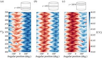
Although we cannot access sidewall temperatures in experiments, we can in simulations, and those temperatures can be useful for characterising the LSC dynamics (Horn et al. Reference Horn, Schmid and Aurnou2021). Plots of the temporal evolution of sidewall temperatures in simulations (Hovmöller diagrams), at heights  $H/4$,
 $H/2$ and
 $3H/4$, are shown in figure 10. Our simulations demonstrate the typical JRV behaviour at
 $\varGamma = 1.4$,
 $Ra = 1.2 \times 10^6$; a single period of hot and cold alternation shows that one convection roll is present, while the characteristic accordion shapes of the hot and cold patches indicate the presence of the JRV mode (Horn et al. Reference Horn, Schmid and Aurnou2021). The black lines give the orientation of the LSC based on an extended sinusoidal fitting
 \begin{equation} T_\psi(\theta)=A \cos(\psi-\theta)+B \cos(2(\psi-\theta))+T_{avg} , \end{equation}
in which  $A$ and
 $B$ are the amplitude of the cold and hot sidewall signals and
 $T_{avg}$ is the average sidewall temperature at mid-height. We use this fitting function to find the orientation of the LSC in the DNS. Similar to the experiments, the LSC remains fixed at an orientation of
 $\mu _{LSC}\approx -57^\circ$. The standard deviation of the angle of orientation is smaller from the fit data, with a value of 9.9
 $^{\circ }$. This is likely due to the lower variability of the temperature compared with the velocity, and the readings being taken from the circumference which is at the boundary layer.
Variation of sidewall temperature with angular position  $\theta$ and time
 $t$ (Hovmöller diagrams) in simulations of the
 $\varGamma = 1.4$ case at
 $Ra = 1.18 \times 10^{6}$. (a) Height
 $z = H/4$; (b)
 $z = H/2$; (c)
 $z = 3H/4$. The characteristic ‘accordion’ shape of the warm and cold regions as they evolve in time demonstrates prominence of the JRV mode (Horn et al. Reference Horn, Schmid and Aurnou2021). Black curves indicate the orientation of the LSC.

3.5. Separating the modes
Next, we examine the different sets of frequency peaks shown in figure 8 separately. Since these peaks appear consistently across multiple diagnostics, at different positions in the vessels and at different container aspect ratios, we posit that they correspond to different container-scale flow modes.
3.5.1. Main peak
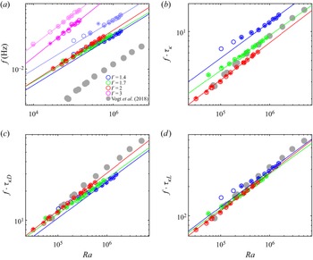
The most prominent peak in the majority of  $1.4 \le \varGamma \le 2$ cases is associated with the JRV frequency. In figure 11(a) we plot peak frequencies vs
 $Ra$ over all
 $\varGamma$ values. For each
 $Ra$, we take the average peak frequency over all temperature data to produce one point,
 $f_0^T$ (stars on the plot) and the average peak frequency over all velocity data to produce the other,
 $f_0^U$ (circles on the plot).
Frequency  $f_0$ of the strongest spectral peak in each convection case, as measured (a), normalised by the thermal diffusion time
 $\tau _\kappa$ (b), normalised by a diameter-based diffusion time
 $\tau ^D_{\kappa } = D^2/\kappa$ (c) and normalised by a path length-based diffusion time
 $\tau ^L_{\kappa } = L^2/\kappa$, all varying with
 $Ra$ (d). Each frequency is an average from all velocity probes
 $f_0^U$ (circles) or all temperature probes
 $f_0^T$ (stars). Secondary peaks
 $f_1$, appearing at
 $\varGamma = 1.4$ and 3, are drawn in lighter colours in (a). Colours represent aspect ratio following figure 4. Experimental frequency peaks from Vogt et al. (Reference Vogt, Horn, Grannan and Aurnou2018) are included as grey circles. The dimensions of their set up are
 $D_{RoMag} = 20$ cm and
 $H_{RoMag} = 10$ cm. Best-fit trends over both temperature and velocity data are plotted as coloured lines with fits given in table 1. Best-fit trends between
 $f_0$ and
 $Ra$ become nearly identical when compensated by
 $\tau ^L_{\kappa }$, but are also effectively collapsed by
 $\tau ^D_{\kappa }$.

To quantify how the JRV frequency varies with  $Ra$, we define
 $f_0$ as the average between
 $f_0^T$ and
 $f_0^U$ in each case and determine its power-law scaling against
 $Ra$ at each
 $\varGamma$. The
 $f_0$ vs
 $Ra$ trend varies at lower
 $Ra$, but a power-law scaling appears at high
 $Ra$. This tendency is most apparent in frequencies normalised by
 $f_{ff}$ (plotted in the second column of figure 8) as discussed above. To omit the low
 $Ra$ regions, we include only data points obeying the following criterion at each aspect ratio:
 \begin{equation} \left| \frac{f/f_{ff} - \left(f/f_{ff}\right)_{end}}{\left(f/f_{ff}\right)_{end}} \right| \le 0.10 , \end{equation}
where ‘ $| \,{\cdot }\, |$’ indicates absolute value and
 $(f/f_{ff})_{end}$ corresponds to the normalised frequency for the highest
 $Ra$ case at a given
 $\varGamma$ (i.e. a point where the
 $f/f_{ff}$ vs
 $Ra$ trend has flattened out). Apart from
 $\varGamma = 3$, the resultant power-law trends are in close agreement in both prefactor
 $c_f$ and exponent
 $\gamma$ (see table 1). In fact, the prefactors and exponents generally lie within the 95 % confidence bounds of each other. The secondary peaks appearing at
 $\varGamma = 1.4$ and 3 are also plotted in in lighter colours. They scale similarly to the primary peaks, but with larger prefactors (see table 1).
Table containing the prefactor and exponent of the power-law fits for  $Re_{LSC}$ vs
 $Ra$ and frequency peaks
 $f_0$ and
 $f_1$ vs
 $Ra$, at each aspect ratio
 $\varGamma$. We chose
 $Re_{LSC}$ since it collapses the data best for
 $1.4 \le \varGamma \le 2$ where the JRV is dominant, and also produces a power-law trend when
 $\varGamma = 3$.

Figures 4 and 11 together demonstrate that both the JRV frequency  $f_0$ and the Reynolds number
 $Re$ scale roughly as
 $Ra^{0.4}$. This agrees with a host of previous studies which find that oscillation frequencies associated with the LSC are directly proportional to the typical flow velocity (Ahlers et al. Reference Ahlers, Grossmann and Lohse2009). Following this, previous studies define a diffusive time scale
 $\tau _\kappa = H^2/\kappa$ and posit that a characteristic scaling of
 \begin{equation} c_{f\tau_\kappa} \tau_\kappa f_0 = c_{Re} Re \end{equation}
should relate the flow speed to oscillation frequencies, where  $c_{f\tau _\kappa }$ depends on the container geometry (Ahlers et al. Reference Ahlers, Grossmann and Lohse2009; Vogt et al. Reference Vogt, Horn, Grannan and Aurnou2018).
In figure 11(b) we compensate the JRV frequencies  $f_0$ by the diffusive frequency
 $\tau _\kappa$. It becomes immediately clear that
 $f_0\tau _\kappa$ varies significantly more with
 $\varGamma$ than
 $f_0$ alone in panel (a). It does, however, bring the
 $\varGamma = 2$ JRV frequencies from Vogt et al. (Reference Vogt, Horn, Grannan and Aurnou2018) into close proximity to our
 $\varGamma = 2$ data. In panel (c) we compensate
 $f_0$ by
 $\tau ^D_\kappa = D^2/\kappa$, a diffusive time scale associated with the horizontal extent of the container rather than vertical. This replicates the close agreement between
 $f_0$ trends, of course, since
 $D$ is constant. However, the agreement between Vogt et al. (Reference Vogt, Horn, Grannan and Aurnou2018) is also carried over from (b) – the vessel size is certainly important to meaningfully scale the JRV frequency. Finally, in (d), we find that
 $\tau ^L_\kappa = L^2/\kappa$ collapses
 $1.4 \le \varGamma \le 2$ data into what is effectively a single trend. This diffusive time scale is associated with the total path length
 $L$ of the JRV motion. This implies that, when using the correct length scale to define
 $\tau _\kappa$, the prefactor
 $c_{f\tau _\kappa }$ is actually constant with respect to aspect ratio. A best-fit scaling across all relevant data produces
 $c_{f\tau _\kappa } = 1.8^{+0.6}_{-0.9}$. The fact that data are largely collapsed by horizontal time scales may indicate that the horizontal dimension is generally more important to the JRV dynamics. This view is consistent with the arguments presented by figure 9.
3.5.2. Secondary peak
As shown in figures 8 and 11, a secondary peak  $f_1$ manifests at
 $\varGamma = 1.4$, distinct from both the fundamental JRV peak and its harmonic. Faint signatures of the peak also appear at
 $\varGamma = 1.7$ and 2. The frequency
 $f_1$ approximately scales with
 $Ra^{0.4}$ and thus stays proportional to the JRV frequency, exceeding it by a factor of
 $1.7 \pm 0.1$.
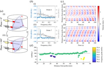
Because the secondary peak appears most prominently in measurements from probes 6 and 7 (see figure 7), we focus our attention there. Probes 6 and 7 are located directly above and below one another, at heights  $3H/4$ and
 $H/4$, and in chord positions, meaning that they can detect azimuthal motions in the LSC. Figure 12 shows that the oscillatory patterns are offset in time by a phase difference of
 $180^\circ$. In figure 12(b) the power spectral density of the velocity measured by probe 6 (b (i), grey) shows that the secondary frequency peak present is clearly distinct from the JRV fundamental frequency and its first harmonic. The same secondary frequency peak appears in probe 7 (b (ii), grey). To examine in detail the dynamics associated with the secondary peak, we apply a bandpass filter that attenuates measurements of flows at other frequencies. The power spectral density of the filtered velocities in figure 12(b) (blue) for probes 6 and 7 shows a single narrow peak at the secondary frequency that excludes the first harmonic of the JRV frequency, as expected. The filtered velocity as a function of position and time is plotted in figure 12(c) for probe 6 (panel c (i)) and probe 7 (panel c (ii)). The filtered velocity profiles are periodic and have opposite orientations at the two probes. Supplementary movie 3 shows filtered velocity measurements from probes 6 and 7, in which the anti-symmetric variations associated with a twisting motion are clear. We calculated the spatial variation of the phase difference, at the secondary frequency, between velocities measured by probes 6 and 7 in figure 12(d). To estimate the phase of each signal, we took the imaginary part of its discrete Fourier transform. The phase difference, at the secondary peak, is uniformly near 180
 $^\circ$.
(a) Schematic of probes 6 and 7 detecting the torsional mode. (b) Power spectral density of the velocities in the  $\varGamma = 1.4$,
 $Ra = 9.77 \times 10^{5}$ case as measured by probes 6 and 7 (grey) and after bandpass filtering around the secondary peak (
 $\approx 0.055$ Hz) (blue). (c) Variation of velocity with position and time, as detected by probes 6 (i) and 7 (ii), after filtering. (d) Phase difference between the measurements on probes 6 and 7 at the secondary frequency peak, varying with distance from the probe. The phase difference is almost constant at
 $180^\circ$ (dashed line) throughout space.

Thus, we posit that the secondary peak is a manifestation of the torsional mode of the LSC. As shown in figure 1 and again in figure 12(a), the torsional mode involves azimuthal twisting motions which would not register on horizontal radial probes, consistent with the fact that spectra of probes 1, 2, 3 and 4 (not shown) have no significant peak at the secondary frequency. A clockwise twist in the upper half of the fluid layer coincides with a counterclockwise twist in the bottom half; the former motion provides a small positive component to probe 6 velocities and the latter a small negative component to probe 7 velocities. The second half of the oscillation period gives the inverse motions on probes 6 and 7. The periodic velocities in probes 6 and 7, offset in phase by 180 $^\circ$, are consistent with this description. Although probe 5 is also in a chord position, it is located at height
 $H/2$, where the torsional mode causes negligible motion. Accordingly, its spectrum has no significant peak at the secondary frequency, either (see figure 7g). This behaviour is also distinct from the JRV motion; filtering the same measurements with a passband around the main peak
 $f_0$ yields a phase difference of mostly
 $25^\circ$ that varies with spatial position (not shown, see supplementary movie 4).
A surprising feature of this torsional mode is the fact that its frequency is separate from the JRV frequency. Horn et al. (Reference Horn, Schmid and Aurnou2021) found that each of the JRV, sloshing and torsional modes occur at similar frequencies and can only be separated through dynamic mode decomposition. Likewise, our simulations reveal no spectral peaks apart from the JRV and its harmonic. A possible explanation is that the torsional peak we observe is actually a harmonic of the fundamental torsional mode, which would exist in even closer proximity to the fundamental JRV peak and may be masked by it. In any case, we believe that ours are the first experimental observations of the torsional mode and JRV mode operating simultaneously.
4. Conclusion
Convection in liquid metals is an ever-relevant topic to geophysical, astrophysical and industrial applications. In this work, we investigated the dynamics of the LSC, which is the fundamental mode of liquid metal convection and can be robust even in the presence of other flow drivers such as magnetic fields (Yanagisawa et al. Reference Yanagisawa, Hamano and Sakuraba2015; Tasaka et al. Reference Tasaka, Igaki, Yanagisawa, Vogt, Zuerner and Eckert2016; Akashi et al. Reference Akashi, Yanagisawa, Tasaka, Vogt, Murai and Eckert2019). Our survey of convection shows robust  $Re$ vs
 $Ra$ scaling consistent with previously published values regardless of aspect ratio. Deriving
 $Re$ from a three-dimensional velocity measured on the central axis at height
 $3H/4$ (in the
 $\varGamma = 1.4$, 1.7 and 2 cases) or height
 $2H/3$ (in the
 $\varGamma = 3$ case),
 $U_{3D}$ collapses the velocities over the full
 $\varGamma$ range and compares well with previously published values (Scheel & Schumacher Reference Scheel and Schumacher2017; Zürner et al. Reference Zürner, Schindler, Vogt, Eckert and Schumacher2019). The horizontal two-dimensional velocity at the same location,
 $U_{LSC}$, approximates the flow speed of the LSC. It collapses
 $Re$ values even more effectively over
 $1.4 \le \varGamma \le 2$, excluding
 $\varGamma = 3$ where the flow is not dominated by a single LSC roll.
By delving into spectral data and the orientation of the LSC plane, we infer that the JRV frequency and morphology may depend only weakly on container height. A couple of separate results support this claim: first, at  $\varGamma = 2$ the LSC plane occasionally orients itself at a 180
 $^\circ$ offset from its primary position in nearly every case (figure 9). We interpret this to mean the vortex core occasionally passes over the probe beam at height
 $3H/4$. This behaviour is entirely absent at
 $\varGamma = 1.4$, indicating that the JRV core circulates around a smaller path relative to the container height. Second, when normalised by
 $\tau _\kappa = H^2/\kappa$, the scaling of the JRV frequency
 $f_0$ varies significantly with
 $\varGamma$ (figure 11). The raw frequency data
 $f_0$, and therefore also
 $f_0/D^2/\kappa$, nearly follow a common best-fit scaling, with prefactors and exponents within 95 % confidence intervals. One way to interpret this is that the horizontal dimension plays a larger role in determining the JRV frequency and than the vertical dimension.
The best collapse of JRV frequency with  $Ra$ over the entire JRV-dominated range
 $1.4 \le \varGamma \le 2$ is produced by considering a diffusive time scale proportional to total path length
 $L^2/\kappa$, which indicates that the scaling between
 $Re$ and JRV frequency is related by a common prefactor of
 $c_{f\tau _\kappa } = 1.8^{+0.6}_{-0.9}$, regardless of
 $\varGamma$. Denser surveys over larger
 $Ra$ ranges could serve to reduce the uncertainties on this prefactor.
Despite the fact that varying the aspect ratio has only weak effects on  $Re$, JRV frequency and perhaps JRV morphology, other dynamical markers demonstrate sensitivity to
 $\varGamma$. For
 $\varGamma = 1.4$, a robust secondary peak appears in the velocity spectra, one which is largely absent for
 $\varGamma = 1.7$ and 2. Using bandpass filters to single out this peak, we see it is best described as a torsional motion. The increasing prominence of such a torsional mode as
 $\varGamma$ approaches 1 is consistent with the DNS results of Horn et al. (Reference Horn, Schmid and Aurnou2021) and speaks to the
 $1 \le \varGamma \le 3$ range of geometries containing rapid shifts in flow morphology.
A remaining mystery is the separation between the frequencies of the torsional-style mode and the JRV mode. Taken at face value, this appears to run counter to previous studies where all LSC modes occur at similar frequencies (Brown & Ahlers Reference Brown and Ahlers2007; Horn et al. Reference Horn, Schmid and Aurnou2021). This topic is certainly worth future experimental and numerical investigation.
At  $\varGamma = 3$, many of the single-roll LSC behaviours appear to break down, giving way to a multi-roll system prone to reversals. The LSC orientation is mostly fixed for aspect ratios
 $1.4 \le \varGamma \le 2$ but varies for
 $\varGamma = 3$. The spectra at
 $\varGamma = 3$ also paint a distinct picture compared with other geometries: the JRV mode seems absent, the primary peak is broader and less consistent in frequency and a secondary peak surfaces at approximately 1.4 times the frequency of the primary peak.
An attractive trajectory for future work is to expand our understanding at  $\varGamma = 3$ and investigate aspect ratios in the range of
 $2 \le \varGamma \le 3$; our data indicate that a transition away from the dominant JRV mode should occur here, yet the nature of this transition remains unclear. The decreased importance of the JRV at
 $\varGamma = 3$ could be interpreted to contrast with the results of Akashi et al. (Reference Akashi, Yanagisawa, Sakuraba, Schindler, Horn, Vogt and Eckert2022), where the JRV dominates in aspect ratios as large as 5, but the difference in vessel shape (cylindrical vs cuboid) confounds any direct comparison. Further investigation into the frequency spectra at
 $\varGamma = 3$ could be particularly helpful; bandpass filtering around the peaks does not yield an easily interpretable picture of the morphology. In general, convective flows at low
 $Pr$ demonstrate rapid transitions in the dominant flow modes over a compact range of aspect ratios between 1 and 3.
Supplementary movies
Supplementary movies are available at https://doi.org/10.1017/jfm.2022.778.
Acknowledgements
The simulation work was carried out with the support of an Australian Government Research Training Program (RTP) Scholarship. Computations were performed on the super-computer Gadi with the assistance of resources and services awarded to project QP46 from the National Computational Infrastructure (NCI), which is supported by the Australian Government.
Funding
This work was supported by the National Science Foundation (grant numbers CBET-1552182 and CMMI-1562545).
Declaration of interests
The authors report no conflict of interest.
Appendix
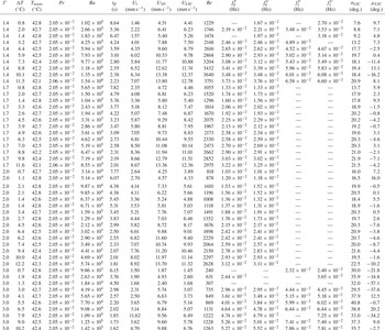
Table containing experimental convection cases. Here,  $\varGamma$ refers to aspect ratio,
 $\Delta T$ is the vertical temperature difference,
 $T_{mean}$ is the mean temperature,
 $Pr$ is the Prandtl number,
 $Ra$ is the Rayleigh number,
 $t_{ff}$ is the free-fall time scale,
 $U_r$ is the typical velocity estimate from UDV probe 1,
 $U_{3D}$ is the typical velocity estimate given by (3.1),
 $U_{LSC}$ is the typical velocity estimate given by (3.2) and
 $Re$ is the Reynolds number. Also,
 $f_0^T$ is the mean peak frequency averaged over temperature probes for the main frequency peak as shown in figure 11. Similarly,
 $f_0^U$ is the same quantity from the UDV probes;
 $f_1^T$ and
 $f_1^U$ correspond to the mean frequency of the secondary peak averaged over temperature and velocity probes, respectively. Finally,
 $\sigma _{LSC}$ is the standard deviation of the LSC orientation
 $\theta$ and
 $\mu _{LSC}$ is the mean value of
 $\theta$ as defined in § 3.4.