1. Introduction
Decision making typically requires judgments about causal relations. Home owners need to know whether putting locks in their doors will make their houses more secure. Jurors need to know whether the accused is causally responsible for damages before they can assess whether he or she is legally responsible. Aid agencies need to know how the different projects they can invest in will affect the lives of those they are concerned about, and so on. Opinions about the nature and strength of causal relations often differ, even among experts. How to handle such diversity of opinion is the topic of this article. We investigate the possibility of coherently aggregating different causal judgments into a single one that may be applied to the decision problem at hand.
The basic setup of this aggregation problem is as follows. Individuals make judgments about both the nature of the causal relations between the variables in some set V = {V, W, …} and the probabilities of these variables taking certain values, unconditionally or conditionally, on the values of other variables. The task is to construct a single aggregate judgment on the causal relations between the variables and the relevant probabilities in a way that preserves, as much as possible, the information contained in the individuals’ judgments. For present purposes, we assume that individuals’ judgments are coherent. More generally, one might allow (localized) incoherence in some of the individuals’ judgments or allow that individuals do not make judgments about all causal relations or all probabilities in question. Their judgments could be restricted to just certain variables relevant to the decision problem at hand or, further still, to just some subset of them or just one type of judgment: causal or probabilistic.
The causal judgments of individuals could be represented in a number of different ways, but here we adopt the framework familiar from the work of Pearl (Reference Pearl2000), Spirtes, Glymour, and Scheines (Reference Spirtes, Glymour and Scheines2000; see also Glymour, Spirtes, and Scheines Reference Glymour, Spirtes and Scheines1990), and others, in which they are represented by Bayesian networks: directed acyclic graphs (DAGs) with associated conditional probabilities. We do not intend thereby to take a position on the nature of causal judgments or on the question of whether they can ultimately be analyzed probabilistically.Footnote 1 Anyone who holds the view that causal judgments are just features of probability judgments—for instance, that to judge that X causes Y is to hold certain conditional probability judgments, such as that the conditional probability of Y given X exceeds its unconditional probability—is free to regard the Bayesian network representations as adding no information to the underlying probability judgments. In principle, we could also study the aggregation of causal judgments in another framework, for instance, by representing causal judgments as counterfactual beliefs of the right kind.
A DAG represents an individual’s qualitative judgment of causal relevance and irrelevance between variables. Her quantitative judgment of causal dependence is reflected in the associated conditional probabilities for the values of these variables, given the values of any variables on which they are directly causally dependent. The individual’s unconditional probabilities for the values of the given variables can then be computed from their conditional probabilities together with the individual’s unconditional probabilities for the parent variables. Consider the following example, which we will use at various points in the discussion.
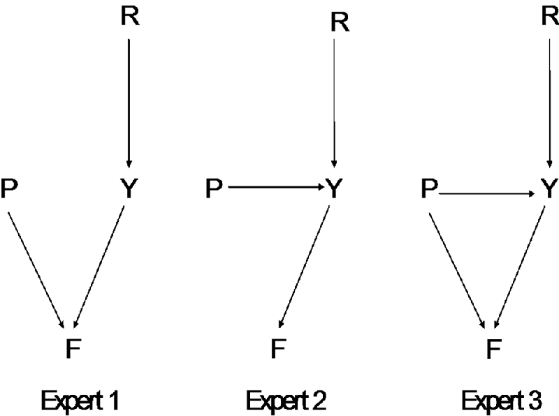
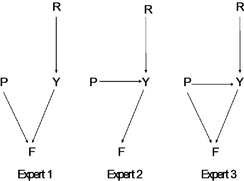
Example: Predicting Famine.— An aid agency wishes to do some advance planning for its famine relief operations and consults several experts in order to determine the risk of famine in a particular region. All agree that the relevant variables are R: rainfall, Y: crop yields, P: political conflict, and of course F: famine. But they disagree both on the causal relations between the four variables and on the probabilities of the various values that these variables may take. All consider rainfall to be the main determinant of crop yield. However, while Expert 1 thinks that poor crop yield and disruptive political conflict are the main causes of famine, Expert 2 thinks that the causal influence of political conflict on famine is indirect, via the effect of the disruption of agricultural production on crop yields. Expert 3 considers the relationship between political conflict and famine to be more complicated still, with political conflict both causing famine directly, by disrupting food distribution, and indirectly, through the influence on crop yields. These three opinions are represented in figure 1 by a set of DAGs.
Expert causal judgments.
The fact that individuals make both causal and probabilistic judgments raises the question whether aggregation of both kinds of judgments should be conducted all at once or in two stages. In section 2, we focus on what we call one-stage aggregation, in which only probability judgments are aggregated. This approach draws on the standard literature on probabilistic opinion pooling (as reviewed, e.g., by Genest and Zidek Reference Genest and Zidek1986). It is motivated mainly by the thought that the probability judgments of individuals reflect their causal judgments in various ways and hence that the problem of causal judgment aggregation may be solved by constraining probability aggregation so as to preserve the causal information contained in probability judgments. Our verdict on this possibility, however, is largely negative. In sections 3–5, we therefore pursue an alternative two-stage approach, aggregating first the qualitative causal judgments represented by the DAGs (sec. 3) and then the quantitative probabilistic ones (sec. 4 and 5), on the assumption that a consensus about the causal relations between variables has been reached. Our analysis builds on results from the literature on binary judgment aggregation, which combines ideas from social choice theory with ideas from logic.Footnote 2
2. One-Stage Aggregation
The problem of aggregating causal judgments has not received much attention, at least in the form presented here, but there is a vast literature on aggregating expert opinions, mainly in statistics, and especially on aggregating expert probabilities. (As already mentioned, an excellent guide to that literature is the survey paper of Genest and Zidek [Reference Genest and Zidek1986].) In this section, we draw on this literature to examine the possibility of reasonable one-stage aggregation of several individuals’ judgments. One-stage aggregation may be the only method available in cases in which individuals make no explicit causal judgments or their causal judgments are very incomplete. It is natural, moreover, for those holding a probabilistic view about causation to rely on this method. But one-stage aggregation may also be motivated by the less controversial thought that the causal judgments of individuals are reflected in (even if they are not reducible to) the relations between the individuals’ unconditional and conditional probabilities for the relevant events. If this is so, then even on a nonreductionistic view about causal judgments one may hope that probability aggregation could be constrained in a manner that preserves the causal judgments implicit in probabilistic ones.
Broadly, there are three classical approaches to probability aggregation: linear pooling, geometric pooling, and supra-Bayesian approaches. The last approach is directed at a problem slightly different from ours—namely, that of how an individual expert should modify his judgments in light of the expressed judgments of other experts—and so we can set it aside. The other two approaches assume that the experts’ opinions have reached an equilibrium state and that no further modification of their viewpoints will take place before the relevant decision has to be made.
Consider an opinion aggregation problem of the following form. A set of events is given (e.g., the event “high political conflict” or “low political conflict and famine”), and the task is to merge the probability judgments of individuals 1, … , n (the “experts”) on these events into an aggregate probability judgment on the events.Footnote 3 So, we have to merge (individual) probability functions Pr1, … , Prn into an (aggregate) probability function Pr. Many aggregation rules are imaginable. Formally, a probability aggregation rule is a function that assigns to each n-tuple 〈Pr1, … , Prn〉 (called a profile) of individual probability functions an aggregate probability function Pr.
Of the various possible aggregation rules, linear pooling stands out for a variety of formal and conceptual reasons (e.g., Aczél and Wager Reference Aczél and Wagner1980; Lehrer and Wagner Reference Lehrer and Wagner1981; McConway Reference McConway1981; Dietrich and List Reference Dietrich and List2007b). In particular, the following axiomatic argument can be given. Let us require the aggregation rule to satisfy two seemingly natural conditions:
Ind.— (Event-wise Independence) The aggregate probability of any given event X depends only on the individuals’ probabilities of X (regardless of the individuals’ probabilities of other events Y).Footnote 4
ZP.— (Zero Preservation) The aggregate probability of any given event X is zero whenever all individuals give X zero probability.Footnote 5
Applied to the event “famine,” for instance, Zero Preservation implies that famine is assigned an aggregate probability of zero if all individual experts assign a probability of zero to it. Event-wise independence implies that the aggregate probability of famine depends only on the probabilities that the individual experts assign to that event, not on the probabilities they assign to a certain level of crop yield, political conflict, and so on. (This is not to deny, of course, that individuals form their judgments regarding famine in light of their judgments on crop yield, political conflict, etc.)
Perhaps surprisingly, the only aggregation rules satisfying these two conditions are linear pooling functions: the aggregate probability of any event X is a (possibly weighted) arithmetic average of the individual probabilities of X; that is,

where the weights w 1, … , wn ≥ 0 add up to one and are the same for all events X (Aczél and Wager Reference Aczél and Wagner1980; McConway Reference McConway1981).Footnote 6 Examples of linear pooling functions are equal-weight averaging (w 1 = … = wn = 1/n) and dictatorial aggregation (some individual i has weight wi = 1, and all others have weight 0).
The natural interpretation of these weights is in terms of judgmental competence, so that the choice of a particular linear pooling rule is dictated by considerations of the relative expertise of the individuals whose opinions are being sought. In this light, the fact that linear pooling rules assign weights to the opinions of individuals that are independent of the object of these opinions seems quite unsatisfactory, since individuals may be more or less expert on different kinds of issues, and it would seem natural to vary the weights on their opinions to reflect this. The aid agency would do well to consult climatologists, agriculturalists, and political scientists to reach a balanced view on the causes of famine, but in doing so it would be reasonable for it to give more weight to the climatologists’ probabilities for rainfall than to the political scientists’ but more weight to the political scientists’ probabilities for political conflict.Footnote 7
Our main concern here, however, is with the question of whether linear pooling functions satisfactorily respect the causal knowledge of the individual experts. An individual’s causal judgments will be reflected in certain (unconditional or conditional) independencies in his or her probability judgments. For instance, if individual i believes that events X and Y do not causally affect each other but have a common cause Z (and have no other common causes, except for those that affect X and Y via Z), then he or she will take X and Y to be probabilistically independent given Z,Footnote 8 because any probabilistic correlation between X and Y is “screened off” by conditionalizing on Z. A minimal requirement of respecting causal judgments is that at least unanimously held causal judgments be reflected in the aggregate probability function Pr. That is, Pr should display at least those (conditional) independencies that are supported by unanimous causal judgments. For example, if all individuals judge X and Y to be causally independent with common cause Z, then that independence judgment should be reflected in the aggregate probability function Pr. This motivates the following condition on probability aggregation:
IP.— (Independence Preservation) For any given events X, Y, Z, if all individuals judge X and Y to be probabilistically independent given Z, then this conditional independence also holds under the aggregate probability function.Footnote 9
Note that, by preserving all unanimous probabilistic independencies (conditional or unconditional), we may also preserve independencies that are not grounded in unanimous causal judgments. For instance, it may be that all individuals judge X and Y to be independent given Z, but some do so on the grounds of judging that X indirectly causes Y through Z, others on the grounds of judging that Y indirectly causes X through Z, still others on the grounds of judging that X, Y, and Z are entirely causally disconnected. Even in this case of causal disagreement, Independence Preservation requires the preservation of probabilistic conditional independence. The purely probabilistic informational basis of one-stage aggregation does not allow us to distinguish between different motivations (causal or other) behind probabilistic independencies. Without explicit causal information, all we can do is to use Independence Preservation to preserve all unanimous causal judgments, at the cost of preserving even those conditional independencies that are not causally motivated.
It turns out, however, that Independence Preservation is violated by all linear pooling functions (unless some individual i gets maximal weight wi = 1) and thus by all nondictatorial probability aggregation rules satisfying Event-wise Independence and Zero Preservation. This fact, proven in Genest and Wagner (Reference Genest and Wagner1984), can be illustrated by using our earlier example.Footnote 10 Suppose the aid agency consults a couple of experts in order to determine the risk of famine in a particular region and that both experts agree that famine is caused by a combination of drought (the event of rainfall R below some critical threshold) and political instability (the event of political conflict P above some critical threshold), which undermines local solutions to poor crop yields. Furthermore, they agree that these two factors are both causally and probabilistically independent, at least in the short term. But they disagree on the probability of drought and of political instability. Since neither speaks with greater authority than the other, the aid agency calculates its probabilities for these events by taking the linear average of the judgments of the two experts.
Let D and I, respectively, denote the occurrence of drought and political instability in the region and DI their concurrence. Let Pr1, Pr2, and Pr, respectively, be the probability functions of Expert 1, Expert 2, and the aid agency. Since pooling happens by averaging, the aid agency will assign the following probabilities:

where the last identity uses the experts’ judgments that D and I are independent. These independence judgments are preserved if and only if Pr(DI) = Pr(D) Pr(I); that is, if and only if

By multiplying both sides of this equation by 4, developing the product on the right-hand side, and simplifying, it follows that

The latter can hold only if Pr1(D) = Pr2(D) or Pr1(I) = Pr2(I), that is, if the experts agree on the probability of drought or of political instability—which is not the case by assumption. So equal-weight linear pooling violates Independence Preservation. Similar violations can be constructed for nonequal weights (unless one individual i gets maximal weight wi = 1).
While we have focused on linear pooling as a way of aggregating probability judgments, the difficulty with preserving causal insights at the aggregate level is a very general one. Genest and Wagner (Reference Genest and Wagner1984) have shown that Independence Preservation is violated by many (linear or nonlinear) probability aggregation rules, including geometric averaging, the most prominent alternative to linear averaging. Thus, the difficulty of preserving causal knowledge is not an artifact of requiring Event-wise Independence (a condition violated, e.g., by geometric averaging).
Genest and Wagner (Reference Genest and Wagner1984) interpret this finding as evidence that Independence Preservation is not a reasonable condition. We would not like to go so far. In our view, those unanimous independence judgments that are grounded in unanimous causal judgments about the world should not be overruled. We take Genest and Wagner’s impossibility finding not as a reason to abandon the goal of preserving judgments of independence but as a reason to move to a two-stage approach that explicitly takes qualitative causal judgments into account.
3. Two-Stage Aggregation: The Qualitative Stage
Under our proposed two-stage approach to aggregation, qualitative causal judgments are aggregated first, and quantitative, probabilistic ones only subsequently. Furthermore, the latter are aggregated in a way that differs from standard probability aggregation, namely, in a way that is constrained by the qualitative causal judgments formed at the first stage. This two-stage approach will satisfy a version of Independence Preservation restricted to unanimously held causal independencies.
As before, let V = {V, W, …} be a (finite) nonempty set of variables. In our example of the aid agency above, V contains the variables R (rainfall), Y (crop yields), P (political conflict), and F (famine). How can we represent qualitative judgments on how the variables in V are causally interrelated? Let us introduce a binary predicate symbol c to represent a causal relevance relation on V, where, for any two variables V and W in V, we write VcW to mean that V is directly causally relevant to W. (For brevity, we speak of “causal relevance,” but we mean “direct causal relevance.”Footnote 11) In the case of the aid agency, an expert who thinks that rainfall is causally relevant to crop yield whereas political conflict is not would hold that RcY but not that PcY. A causal relevance relation c is called acyclic if, for any finite sequence V 1, V 2, … , Vk of variables in V, it is not the case that

A causal relevance relation c induces a directed graph whose vertices are the variables in V and whose edges (arrows connecting vertices) are defined as follows: for any two variables V and W in V, there is an edge from V in the direction of W if and only if VcW. This graph is a DAG if c is an acyclic relation.Footnote 12
A Bayesian network is a DAG with associated conditional probabilities: each variable in the graph is endowed with a conditional probability distribution given its parents in the graph. In this section, however, we set this quantitative information aside and focus on qualitative features of the DAG alone. In particular, we investigate how a group of individuals can arrive at an aggregate judgment on what the causal relevance relation c between the variables in V is.
Consider a group of n individuals, labeled 1, 2, … , n, each of whom holds a particular judgment on the nature of the causal relevance relation between the variables in V. We write ci to denote the causal relevance relation according to individual i’s judgment. A combination of causal relevance relations across the n individuals is called a profile and denoted 〈c 1, c 2, … , cn〉. A causal judgment aggregation rule is a function that assigns to each profile 〈c 1, c 2, … , cn〉 (in some domain of admissible profiles) a single aggregate causal relevance relation c.
To give some examples of causal judgment aggregation rules, consider the class of threshold rules. A threshold rule, with threshold k (where 1 ≤ k ≤ n), assigns to each profile 〈c 1, c 2, … , cn〉 the causal relevance relation c defined as follows: for any two variables V and W in V,

Examples of threshold rules are the majority rule (k = (n + 1)/2), the union rule (k = 1), and the intersection (or unanimity) rule (k = n).
Are these satisfactory causal judgment aggregation rules? It is easy to see that each of these three rules has a considerable defect. The majority and union rules fail to ensure acyclicity of the aggregate causal relevance relation, even when all individuals hold acyclic such relations. To see this, suppose the aid agency consults three experts, with the following individual judgments. They all agree that rainfall is causally relevant to crop yields, but they disagree on the causal relations between the other variables. Expert 1 thinks that crop yields are causally relevant to famine, which is causally relevant to political conflict. Expert 2 thinks that famine is causally relevant to political conflict, which is causally relevant to crop yields. Expert 3 thinks that political conflict is causally relevant to crop yields, which is causally relevant to famine. In consequence, the causal relevance relation generated by the majority rule violates acyclicity: the relation contains a cycle from crop yields to famine to political conflict to crop yields. It is obvious that the union rule has the same defect. The intersection (or unanimity) rule, by contrast, ensures acyclicity of the aggregate causal relevance relation but may generate a sparse or even empty such relation, with few variables deemed causally relevant to any others, whenever there are disagreements between the experts.
Although threshold rules are particularly salient examples of causal judgment aggregation rules, they are by no means the only ones. So let us adopt an axiomatic approach and look for rules satisfying certain conditions.
UD.— (Universal Domain) The causal judgment aggregation rule accepts as admissible any logically possible profile of acyclic causal relevance relations.
AC.— (Acyclicity) The aggregate causal relevance relation is always acyclic.
UB.— (Unbiasedness) For any two variables V and W in V, the aggregate judgment on whether V is causally relevant to W depends only on individual judgments on whether V is causally relevant to W (the independence requirement), and the aggregation rule is neutral between whether or not this is the case (the neutrality requirement).Footnote 13
ND.— (Nondictatorship) There does not exist a fixed individual such that, for every admissible profile of causal relevance relations, the aggregate causal relevance relation is the one held by that individual.
Although these conditions may seem natural at first sight, they are mutually inconsistent.
Theorem 1.— If V contains three or more variables, there exists no causal judgment aggregation rule satisfying UD, AC, UB, and ND.
This result follows from an impossibility theorem by Dietrich and List (Reference Dietrich and List2010a) concerning the aggregation of binary judgments on logically connected propositions. Qualitative causal judgments in the sense investigated here are simply binary (true/false) judgments on propositions of the form “variable V is (or is not) directly causally relevant to variable W,” where different such propositions constrain each other via the acyclicity constraint on causal relevance. For example, the set of propositions {“V is directly causally relevant to W,” “W is directly causally relevant to U,” and “U is directly causally relevant to V”} is logically inconsistent relative to the acyclicity constraint. From the theory of judgment aggregation, we know that the aggregation of binary judgments on logically connected propositions is subject to a family of impossibility results broadly similar to Arrow’s impossibility theorem on preference aggregation, as surveyed in List and Puppe (Reference List, Puppe, Anand, Puppe and Pattanaik2009) and, more recently, List (Reference List2012). Our current theorem belongs to this family of results. What are the possible escape routes from this impossibility?
The First Route: Relaxing Universal Domain
We may use a causal judgment aggregation rule that accepts, as admissible input, not all logically possible profiles of acyclic causal relevance relations but only those that meet an additional structural condition, namely, profiles that, informally speaking, reflect a certain amount of cohesion across different individuals’ causal judgments. The additional structural condition on profiles might be such that the majority rule, or perhaps some other threshold rule, never generates an aggregate causal relevance relation violating acyclicity. In this case, the majority rule or threshold rule in question could be employed on this restricted domain of admissible profiles. We consider two structural conditions of this kind.
Temporal-Order Restriction
Suppose the individuals agree on the temporal order in which the events captured by the variables in V occur. Suppose further they agree that a variable V can be causally relevant to another variable W only if V strictly precedes W in this temporal order. Call any profile of causal relevance relations that is consistent with some such agreement temporal-order restricted. Formally, a profile is temporal-order restricted if there exists some weak order of the variables in V (a reflexive, transitive, and connected binary relation on V) such that, for every pair of variables V and W in V, if some individual judges V to be causally relevant to W (i.e., some i holds VciW), then V strictly precedes W in that order. For any such profile, the causal relevance relation generated by any threshold rule is acyclic, no matter how low or high the threshold is. The temporal constraint on what causal relevance judgments are deemed admissible guarantees the absence of any causal cycles at both the individual and the aggregate levels.
Unidimensional Alignment
Another structural condition on profiles that ensures acyclic causal judgments at the aggregate level—here under the majority rule (or any threshold rule with a higher threshold)—is unidimensional alignment (List Reference List2003; for generalizations, see Dietrich and List Reference Dietrich and List2010b). A profile of causal relevance relations is called unidimensionally aligned if the individuals can be linearly ordered from left to right such that, for each pair of variables V and W in V, the individuals who hold that V is causally relevant to W (i.e., the individuals i with VciW) are all to the left or all to the right of those who hold that V is not causally relevant to W (i.e., the individuals i who do not have VciW).Footnote 14 For any unidimensionally aligned profile, the causal relevance relation generated by the majority rule is acyclic and coincides with the causal relevance relation held by the median individual with respect to the left-right ordering of the individuals. (Or, if the number of individuals is even, it coincides with the intersection of the causal relevance relations held by the two median individuals.)
It is an empirical question whether a group of experts—either before or after a period of joint deliberation—exhibits sufficient agreement in their causal judgments to meet the condition of temporal-order restriction or that of unidimensional alignment. The kind of temporal agreement required for temporal-order restriction seems empirically plausible at least in some situations.
The Second Route: Relaxing Acyclicity
A logically possible way to avoid the impossibility result of theorem 1 is to give up the requirement that the aggregate causal relevance relation be acyclic. This, however, would constitute a major departure from the consensus on the nature of causal relations, which are widely held to be acyclic (Pearl Reference Pearl2000).
The Third Route: Relaxing Unbiasedness
We may use a causal judgment aggregation rule that violates the condition of unbiasedness. There are two ways of relaxing this condition.
A Neutrality Relaxation
If we relax the neutrality part of unbiasedness, there can exist pairs of variables V and W in V such that the aggregation rule is not neutral between whether or not V is causally relevant to W. Examples of causal judgment aggregation rules violating neutrality are threshold rules with any threshold k different from simple majority. It can be shown that a threshold rule is guaranteed to generate an acyclic causal relevance relation if and only if the threshold k exceeds ([m − 1]/m)n, where m is the number of variables in V.
Let us explain why this constraint on the threshold is sufficient to ensure acyclicity. Suppose, for a contradiction, that a threshold rule with a threshold k above ([m − 1]/m)n generates a cyclical causal relevance relation. There must then exist an admissible profile 〈c 1, c 2, … , cn〉 of individually acyclic causal relevance such that

where c is the aggregate causal relevance relation and V 1, V 2, …,  are distinct variables in V, with 2 ≤ m′ ≤ m.Footnote 15 Given the definition of our threshold rule, there must be at least k individuals with V 1ciV 2, at least k individuals with V 2ciV 3, and so on. Let N 1, N 2, … ,
 be the sets of individuals i with V 1ciV 2, V 2ciV 3, … ,
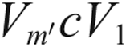 , respectively. Since k exceeds ([m − 1]/m)n, each of these sets must contain more than ([m − 1]/m)n individuals. But, for combinatorial reasons, any m or fewer subsets of size greater than ([m − 1]/m)n from a set of n individuals must have a nonempty intersection. For example, any two or fewer subsets of size greater than (1/2)n must have a nonempty intersection, any three or fewer subsets of size greater than (2/3)n must have a nonempty intersection, and so on. Since m′ ≤ m, this implies that there must exist at least one individual i who is contained in all of N 1, N 2, … ,
 , and he or she must then have

But this contradicts individual acyclicity, which completes the argument.
Conversely, if the threshold k does not exceed ([m − 1]/m)n, it becomes possible to construct an admissible profile 〈c 1, c 2, … , cn〉 of individually acyclic causal relevance relations such that, for some set of distinct variables V 1, V 2, … ,  , each of V 1cV 2, … ,
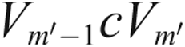 , and
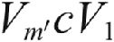 is affirmed by k or more individuals. For such a profile, the intersection of the relevant sets N 1, N 2, … ,
 is empty, and hence the presence of a cycle in the aggregate causal relevance relation does not conflict with acyclicity in the individual relations. Formally, our necessary and sufficient condition for acyclicity (i.e., a threshold k above ([m − 1]/m)n) can be derived from a characterization of consistent (but possibly incomplete) quota rules in judgment aggregation (Dietrich and List Reference Dietrich and List2007a; the current combinatorial argument builds on a result in List [Reference List2001], chap. 9).
Note that if the set of variables V is infinite, only the intersection (or unanimity) rule guarantees acyclicity at the aggregate level. However, if V is finite, then a supermajority rule with a suitably high threshold is sufficient. A problem with this approach, as noted above, is that it may lead to sparse or even empty aggregate causal relevance relations unless the disagreement between experts is limited.
An Independence Relaxation
If we relax the independence part of unbiasedness, there can exist pairs of variables V and W in V such that the aggregate judgment on whether V is causally relevant to W depends not only on individual judgments on whether V is causally relevant to W but also on individual judgments involving other variables. Examples of causal judgment aggregation rules violating independence are sequential priority rules (adapted from List Reference List2004) and distance-based rules (adapted from Pigozzi Reference Pigozzi2006; Miller and Osherson Reference Miller and Osherson2009). Under a sequential priority rule, the different possible pairs of variables are considered one by one in a given order (which may be chosen, e.g., by some criterion of epistemic priority). On each pair of variables V, W, the aggregate judgment is then determined as follows:
i) If the question whether V is causally relevant to W is constrained (in light of the acyclicity requirement) by the aggregate judgments on pairs of variables considered earlier in the given order, then the aggregate judgment on V’s causal relevance to W is derived from those earlier constraints.
ii) If it is not constrained in this way, then the aggregate judgment on V’s causal relevance to W is made by applying some voting method, such as majority voting, to the individual judgments on V vis-à-vis W.
This approach guarantees acyclicity of the aggregate causal relevance relation but at the expense of path dependence: the order in which causal judgments are made on different pairs of variables may determine what the aggregate causal relevance relation will look like. An agenda setter on a committee of experts may strategically exploit this feature of the causal judgment aggregation rule by proposing an order of priority among different pairs of variables that is likely to give rise to aggregate causal judgments that he or she wants the committee to make.
Under a distance-based rule, we first define a distance metric between causal relevance relations. For instance, we could define the distance between two relations c and c′ to be the number of ordered pairs of variables V, W on which c and c′ disagree; that is,  . (This is the Hamming distance.) We then define the aggregate causal relevance relation for any given profile 〈c 1, c 2, … , cn〉 as an acyclic causal relevance relation c that minimizes the total distance from the individual causal relevance relations, that is, where
 is minimal. Since there need not be a unique such distance-minimizing relation c, we may require an additional rule for breaking ties. Distance-based rules can be interpreted as generating compromise causal relevance relations.
In some cases, a rather significant departure from independence (as a property of the aggregation rule) may be desirable. Suppose, for instance, that all individuals agree that there is a causal path from V 1 to V 2, but different individuals disagree about the intermediate variables along this path. Some think that the path goes from V 1 to V 3 to V 2, others think it goes from V 1 to V 4 to V 2, still others think it goes from V 1 to V 5 to V 2, and so on. In such a case, no single causal link between any pair of variables is accepted by more than a small minority of the individuals. If we used a causal judgment aggregation rule satisfying independence, say a threshold rule with a majority or even submajority threshold, we could end up with an empty aggregate causal relevance relation here, without any causal links at all. This would fail to do justice to the fact that all individuals agree that V 1 is at least indirectly causally relevant to V 2. We do not offer a concrete proposal on how to handle such cases but mention it in order to illustrate why a significant relaxation of independence may sometimes be justified.Footnote 16
The Fourth Route: Relaxing Nondictatorship
A final way to avoid the impossibility result of theorem 1 is to allow the aggregate causal relevance relation to be determined by an antecedently fixed individual: a “dictator.” But since we are normally interested in the information contained in the causal judgments of more than one individual, this is not generally an attractive solution to our aggregation problem. Sometimes, however, it may be an acceptable compromise to appoint a trusted expert as the “dictator” for arriving at qualitative causal judgments—in the form of a DAG—while continuing “democratically” when it comes to determining the associated quantitative probability information at the second stage of our two-stage approach.
Concluding Remark
Which of the different possible escape routes from the impossibility result of theorem 1 is compelling depends on details of the decision problem at hand, the nature of the disagreements between the experts, the level of trust we place in them, whether we are worried about possible agenda manipulation, and other factors. In the next section, we assume that through one of the identified routes—excluding that of relaxing acyclicity—a “consensus” on a causal relevance relation and thereby on a DAG has been achieved, and we turn to the question of how the associated conditional probabilities can be determined.
4. Preliminaries to the Quantitative Stage
We have analyzed how a group can arrive at an aggregate judgment on the qualitative causal relations between variables. We now assume that such an aggregate causal judgment has been reached through one of the routes just discussed and suppose that the group seeks to make an aggregate probability judgment (about the variables taking various values) that is compatible with the given aggregate causal judgment.
In its most general form—ignoring for the moment the causal judgment—a probability judgment can be represented by a joint probability function over the variables in V. For simplicity, we assume that each variable can take finitely, or countably infinitely, many possible values. For example, we may distinguish between a particular number of possible levels of conflict. Let us label the variables V 1, … , Vm. A joint probability function Pr assigns a probability  to each combination
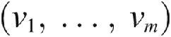 of values of these variables, where the sum of the probabilities is 1.
The joint probability  can be factorized into the product of conditional probabilities:Footnote 17

In our famine example, where V 1, V 2, V 3, V 4 are the levels of rainfall, crop yield, political conflict, and famine, we have

When is the probability judgment expressed by Pr compatible with a given causal judgment? Recall that a causal judgment takes the form of a particular DAG over the variables V 1, … , Vm, with an arrow from Vj to Vk just in case Vj is considered causally relevant to Vk (VjcVk). For any variable Vj, we write PA(Vj) to denote the list of Vj’s parent variables in the graph, and we write pa(Vj) to denote any list of values of these parent variables.Footnote 18
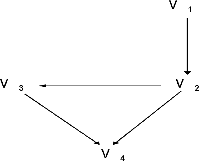
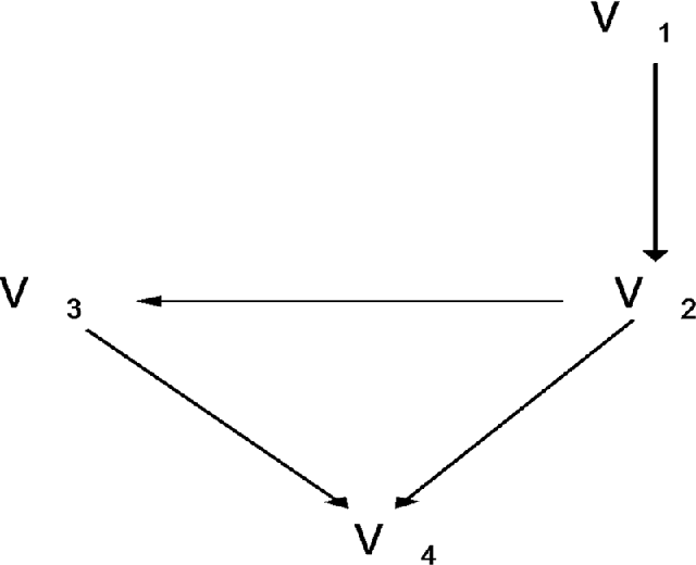
For instance, suppose that the consensus DAG in our famine example is as shown in figure 2: no variable is causally relevant to rainfall (V 1), only rainfall (V 1) is causally relevant to crop yield (V 2), only crop yield (V 2) is causally relevant to political conflict (V 3), but both crop yield (V 2) and political conflict (V 3) are causally relevant to famine (V 4). Then PA(V 1) contains no variable, PA(V 2) contains precisely V 1, PA(V 3) contains precisely V 2, and PA(V 4) contains both V 2 and V 3.
Illustrative aggregate causal judgment in the famine example.
Without loss of generality, suppose the variables V 1, … , Vm are labeled such that those with no parent come first, those with a parent but no grandparent come next, those with a grandparent but no great-grandparent come thereafter, and so on. If the original labeling V 1, … , Vm does not have this property, we can simply relabel the variables appropriately and replace the factorization (1) by one using the new labeling. So the parents of any variable Vj come before Vj.Footnote 19 But of course not all of V 1, … , V j−1 need to be causally relevant to Vj. For instance, in our famine example V 2 but not V 1 is (directly) causally relevant to V 3. Since causally irrelevant variables should have no effect on Vj, the conditional probability  should be insensitive to the nonparental values among
 . In other words, it should be sensitive only to the sublist pa(Vj) of
 . Formally,

We say that the probability judgment Pr is compatible with the given aggregate causal judgment if identity (2) holds for every variable Vj and every combination of values  with
 . (This compatibility requirement is the ordered Markov condition, which is, in turn, equivalent to the parental Markov condition: any variable is independent of its nondescendants given its parents.Footnote 20) The joint probability pa(Vj) then reduces to

For instance, in our famine example,

5. Two-Stage Aggregation: The Quantitative Stage
As we seek to reach an aggregate probability judgment that is compatible with the aggregate causal judgment, the probability function Pr should satisfy the decomposition (3). This requirement is usually violated by standard one-stage probability aggregation, where the individual probability functions

are directly merged into an aggregate probability function  . On our proposed two-stage approach, by contrast, Pr is explicitly constructed so as to meet the necessary decomposition requirement.
Let the aggregate causal relevance relation (the “consensus” DAG) be given, and consider the decomposition constraint (3) relative to that relation. The quantitative stage of our approach now consists in
i) determining each factor of the decomposition,
 , through separate probability aggregation, and
ii) computing the joint probability function
as the product of these separately determined factors.
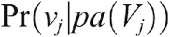 , through separate probability aggregation, and
 as the product of these separately determined factors.
More formally, for every variable Vj in V and every combination pa(Vj) of parental values, we merge the individual conditional probability functions

into an aggregate conditional probability function 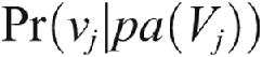 . These separate aggregation exercises can each be performed, for example, by linear or geometric pooling. In our famine example, this involves
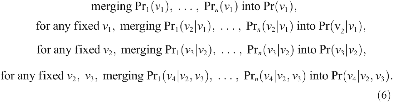
The current approach has several distinctive properties, to which we now turn.
Compatibility with Causal Judgments
The aggregate probability function Pr, given by (3), is automatically compatible with the aggregate causal relevance relation, represented by the appropriate DAG. In particular, Pr respects the causal Markov condition: any variable Vj is probabilistically independent of all its causal nondescendants given its causal parents. In our famine example, Pr makes political conflict independent of rainfall conditional on crop yield,Footnote 21 and famine independent of rainfall conditional on crop yield and political conflict.Footnote 22 The causally motivated conditional independencies are thus respected, whereas other conditional independencies may or may not arise. By contrast, standard one-stage probability aggregation does not generally produce an aggregate probability judgment that is consistent with any prior judgments of causal relevance.
Preservation of Causal (Conditional) Independencies
What about the preservation of unanimously held independencies between variables (both conditional and unconditional ones)? Suppose, for example, that all individuals consider variables Vj and Vk probabilistically independent given Vl.Footnote 23 Does the aggregate probability judgment preserve this conditional independence? As we have seen, for standard probability aggregation methods the answer is usually negative. Under our approach, by contrast, causal conditional independencies are preserved. To see why, suppose all individuals judge Vj and Vk to be probabilistically independent given Vl because of a unanimous agreement that Vj’s only causal parent is Vl and that Vk is not a causal descendant of Vj. Then the aggregate probability judgment respects this independence: according to Pr, Vj and Vk are also probabilistically independent given Vl.Footnote 24 The reason is that, so long as a “reasonable” causal judgment aggregation rule is used at the first stage of our two-stage process, we will have arrived at an aggregate causal relevance relation that reflects the unanimous opinion on the causal relations between Vj, Vk, and Vl; the second stage then leads to a probability function that is compatible with this aggregate causal relevance relation.Footnote 25
Variable Expert Weights
In contrast to one-stage linear or geometric pooling of probabilities, our approach is compatible with the assignment of different weights to different experts’ judgments so as to reflect their different levels of competence on the relevant issues. Once the consensus DAG for the causes of famine is given, for instance, greater weight can be assigned to the climatologist’s judgment in the aggregate probability for rainfall (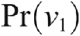 ); to the agriculturalist’s judgment in the aggregate conditional probability for crop yield, given a level of rainfall (
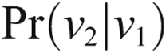 ); and to the political scientist’s judgment for the aggregate conditional probability for political conflict, given crop yields (
 ). In the limit, an aggregate judgment on the probability of famine might be constructed using only the consensus DAG and the judgments of the relevant expert on each variable. But as the literature on epistemic democracy shows, there can be advantages to consulting a range of opinions provided that all who are consulted are sufficiently competent. The two-stage method can be used to optimize the balance between competence and diversity of opinion by suitable assignment of weights in the aggregation of probabilities for each variable.
Complexity Reduction
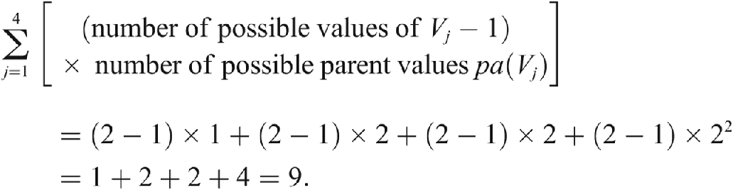
Our two-stage approach subdivides an m-dimensional probability aggregation problem into several one-dimensional ones. Rather than aggregating joint probability functions over the vector V 1, … , Vm (of the form [4]), we aggregate conditional probability functions of a single variable Vj (of the form [5]). But we face several such aggregation problems, namely, one for each variable Vj and each fixed combination of parent values paj(Vj). This is less demanding on the side of individual inputs, as long as the aggregate DAG is not too rich in causal connections. To illustrate this complexity reduction, consider our famine example again, and suppose for simplicity that each variable can take only two values; that is, there are only two levels of rainfall, two levels of crop yield, and so on. If we were to aggregate the joint probability functions  directly, each individual would have to submit 24 − 1 = 15 probability values (there are 24 possible combinations of values
 , but once the probabilities of 24 − 1 of them are specified, the remaining probability is given by one minus the sum of the rest). Specifying any one of these 15 probabilities is hard in practice: what, for example, is the probability of a combination of high rainfall and low crop yield and low political conflict and high famine? Under our approach, by contrast, each individual has to submit only probabilities or conditional probabilities of singular events, like the probability of high rainfall or the conditional probability of high crop yield given low rainfall. The number of required probabilities is smaller than 15 in our example. Using (6), we can see that it equals
Types of Informational Input
Our approach not only reduces the complexity of the aggregation problem; it also uses a different informational input, compared to one-stage probability aggregation. First, we use the additional information of the individuals’ qualitative causal judgments—the information aggregated at the first stage of our two-stage process. Second, an interesting question arises about the nature of the probabilistic input used at the second stage. Consider a variable Vj with parents PA(Vj) in the aggregate causal relevance relation (DAG). Since that relation is the result of the aggregation of individual causal relevance relations, some individuals may not agree that the variables listed in PA(Vj) are the correct causal parents of Vj. They may think instead that not all of these variables are causally relevant to Vj or that some other variables are relevant, despite not being included in PA(Vj). But then, what does such an individual’s conditional probability 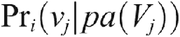 —the informational input at the second stage—represent? For instance, individual 1’s causal relevance relation may be of the form V 1 → V 2 → V 3, while all other individuals’ causal relevance relations may be of the form V 1 → V 2 ← V 3, which might then also become the aggregate relation. Here, individual 1 disagrees with everyone else about both PA(V 2) and PA(V 3). How should we interpret individual 1’s conditional probabilities
 and
 at the second stage of our two-stage aggregation process? Similarly, what is someone supposed to answer to the question “how probable is high political conflict given low crop yield?” if he or she actually thinks that famine rather than crop yield is causally relevant to political conflict?
There are at least three possible interpretations of an individual’s conditional probabilities in such cases: an evidential, a causal, and a hypothetical one. We begin with a discussion of the first two interpretations. To give an informal example, suppose for a moment that, according to individual i’s qualitative causal judgment, the variables in PA(Vj) are not causally relevant to Vj but nonetheless probabilistically correlated with Vj. Then, if 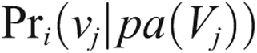 represents an evidential conditional probability, its value is sensitive to pa(Vj) (by probabilistic dependence), whereas if it is understood as a causal conditional probability, its value does not depend on pa(Vj) (by causal independence). More generally, an evidential conditional probability represents an agent’s belief, given a particular evidential supposition (here the supposition that the values of the variables in PA(Vj) are pa(Vj)). A causal conditional probability represents an agent’s belief, given a particular counterfactual supposition (its content again being that the values of the variables in PA(Vj) are pa(Vj)). This causal conditional probability can be understood as resulting from supposing an external intervention in our system that sets the values of the variables PA(Vj) to pa(Vj). The two kinds of conditional probability take the same value if PA(Vj) consists of the correct causal parents according to individual i’s qualitative causal judgment but may differ in general.
Formally, in the evidential case, 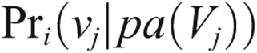 is a standard conditional probability, which can be derived from individual i’s joint probability function over the variables using Bayes’s rule.Footnote 26 In the causal case,
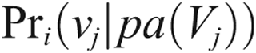 can be calculated as follows (and is sometimes denoted
 or
 to mark the difference; see also Pearl Reference Pearl2000).
i) Modify individual i’s causal relevance relation by deleting relevance links from any variable to any of the variables in PA(Vj). So, the variables in PA(Vj) have no parents left (intuitively, they are set by an external intervention).
ii) Modify the probability assignment to the variables PA(Vj) by letting them take the values pa(Vj) with probability one (unconditionally, since these variables no longer have any parents).
iii) Relative to this new “postintervention” Bayesian network, compute the probability that Vj takes the value
in the usual way. This probability then coincides with the causally understood conditional probability (= ) of the initial Bayesian network.Footnote 27
 in the usual way. This probability then coincides with the causally understood conditional probability
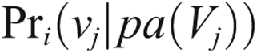 (=
 ) of the initial Bayesian network.
Let us now turn to the third possible interpretation of the individuals’ conditional probabilities submitted at the second stage of our two-stage aggregation process: the hypothetical interpretation. Here, individuals are asked to entertain the hypothesis that the aggregate causal relevance relation is correct and to express conditional probabilities based on this hypothesis. It is unclear, however, whether and how  can be derived from the individuals’ Bayesian networks. This raises a number of challenges for future research.
6. A Final Challenge
The first stage of our two-stage approach restricts the second by requiring the aggregate probability function to display certain conditional independencies mandated by the aggregate causal relevance relation. Roughly, the fewer causal links are accepted at the first stage, the more probabilistic independencies are enforced at the second stage. In the extreme case in which no variable is deemed causally relevant to any other variable, the second stage produces an aggregate probability judgment according to which every variable is probabilistically independent of every other. Accepting few causal connections has the advantage of reducing the complexity of the probability aggregation problem at the second stage but the potential disadvantage of overrestricting the admissible probability assignments. This restriction is problematic when the sparse set of accepted causal links between variables is not a result of the individuals believing in sparse causal links but a result of a causal judgment aggregation rule setting a high threshold for the acceptance of causal links.
We are thus faced with a trade-off between (i) the goal of reducing the complexity of the probability aggregation problem (achieved via a high threshold for accepting causal links between variables) and (ii) the goal of representing causal effects between variables when there are such effects (achieved via a low threshold for accepting causal links). We have argued that a high threshold for accepting causal links may help to prevent a cyclical aggregate causal relevance relation, whereas in other situations, particularly if the variables can be put into a temporal order, even a low threshold (perhaps lower than the majority threshold) guarantees acyclicity. We leave it as a challenge for future research to come up with causal judgment aggregation rules that perform well on both aspects of this trade-off: being neither too permissive nor too restrictive in accepting causal links while avoiding cyclical causal judgments.
 , if for all i, VciW if and only if not
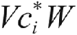 , then VcW if and only if not
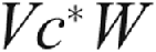 . This formal statement is slightly weaker than the informal one in the main text but implies it under UD and AC.
 can be derived from the joint probability function Pr via the formula
 (where
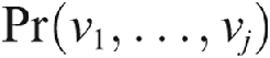 and
 are marginal probabilities derived from Pr), provided that
 . If
 , then
 can be viewed either as undefined or as a primitive not derived from the function Pr. Under both interpretations, the
 is zero whatever value is substituted for
 (because some other factor on the right-hand side of
 .
 .
 .
 .
 , given pa(Vj), according to individual i’s DAG, we would have to redo the calculation described in steps i–iii with the set of variables PA(Vj) replaced by its subset consisting only of variables that are also parents of Vj according to i’s DAG. This subset may be empty, in which case the direct causal conditional probability of
 , given pa(Vj), coincides with the unconditional probability of
 .