1. Introduction

Historically, debates about scientific realism have focused on whether a theory's success in predicting “observable” properties warrants belief in any “unobservable” entities postulated by the theory. One might suppose, therefore, that theories invoking only observable entities should be immune from antirealist skepticism (Musgrave Reference Musgrave, Churchland and Hooker1985). Yet Sober has now repeatedly called for an “instrumentalist” attitude toward hypotheses about such manifestly observable entities as corn plants and lizards (Sober Reference Sober1999, Reference Sober2002; Hitchcock and Sober Reference Hitchcock and Sober2004).

The dearth of published critical responses to Sober's argument may stem partly from the relative novelty of the statistical paradigm in which he framed it. This “Akaikean” statistical framework concerns why a certain kind of simplicity should count in favor of a hypothesis and how to weigh simplicity against goodness of fit (Forster and Sober Reference Forster and Sober1994). These considerations help a scientist choose, from among a small set of alternatives at a given time, the hypothesis that will be the most predictively accurate in the future. Sober's arguments establish that the hypothesis most accurately reflecting the complexity of a given system will not necessarily yield the most accurate predictions about that system. This is a good point, and perhaps an important one for scientists and interested philosophers to keep in mind.

Yet Sober has only shown that predictive success may be a poor guide to one very specific kind of verisimilitude. Use of the term “instrumentalism” invites his readers to conclude that predictive accuracy has no connection to any “deeper” kind of truth (deeper, that is, than predictive accuracy itself). But even in the Akaikean context, accurate predictions are no cosmic accident. They result from accurate parameter values. This connection between the accuracy of predictions and the accuracy of parameter values warrants the type of inference favored by realists, namely, inference to verisimilitude as the best explanation of predictive success. In other words, even if we grant Sober's argument against realism about a certain kind of complexity, realism about parameter values not only survives this argument but can be supported by the same statistical framework in which the argument is couched. Below, I develop this point with a brief introduction to the Akaikean framework, some comments about verisimilitude, and some computer simulations.

2. Parsimony and Statistical Inference

Many philosophers and scientists have espoused a preference for simpler, that is, more parsimonious, theories over more complex ones, at least in certain circumstances. One can imagine various justifications for such a preference. Perhaps nature itself is simple, at least in certain respects; this was Newton's rationale.Footnote ¹ Our own cognitive limitations provide another motive for simplicity. And scientists often consider simpler theories more beautiful than clunkier ones. Aesthetics may thus constrain scientific inquiry, at least somewhat. Forster and Sober (Reference Forster and Sober1994) introduced philosophers to a justification of parsimony that relies on a more precise definition of simplicity than do any of these other rationales. Moreover, this justification does not require nature to be simple, humans stupid, or simple theories especially lovely.

In statistics, one theory, hypothesis, or model is simpler than another if it has fewer adjustable parameters. For instance, the following equation,

is simpler than

Equation (1a) can be used to model the effect of area—A, for example, in square kilometers—on the number of species (S).Footnote ² For example, generally speaking, the greater the area of an island in the Lesser Antilles island chain of the Caribbean Sea, the greater the number of bat species resident on the island. Equation (2a) can model the joint effect of area and isolation—I, in kilometers—on species diversity. Many islands get most of their species from the nearest mainland (Rosenzweig Reference Rosenzweig1995). But the further away that mainland is, the fewer terrestrial species make it across the intervening ocean. Thus, for example, Lesser Antilles islands further away from South America tend to have fewer bat species. S, A, and I are the variables in these equations; c, z, and w are the parameters.

All of the parameters in Equations (1a) and (2a) are adjustable (hence the “a” for “adjustable”). An adjustable parameter is one whose value is not specified in advance—in advance, that is, of the collection and analysis of a particular set of empirical data. Instead, the value of an adjustable parameter is estimated on the basis of those data. Consider bats in the Lesser Antilles again. For these species and islands, application of standard statistical methods (in this case, least squares regression of log-transformed data) to Equation (1a) yields estimates of $c=1.7$ and $z=0.25$ (data from Griffiths and Klingener Reference Griffiths and Klingener1988). Application of the same methods and data to Equation (2a) yields estimates of $c=6.5$ , $z=0.22$ , and $w=-0.18$ . These estimates result in the following fitted models:

and

Models with more versus fewer adjustable parameters have contrasting strengths and weaknesses. Having more adjustable parameters endows more complex models with a kind of flexibility. This flexibility makes them more sensitive than simpler models to the true signal about the effects of certain variables on others (e.g., the effects of area and isolation on number of species). However, this same flexibility also gives more complex models greater sensitivity to noise in the data. Thus, in the process of being fitted to, that is, accommodating, a given data set, a more complex model may actually get so “distracted” by noise that it ends up further from the truth—in a sense to be specified below—than a simpler model. This lesser verisimilitude renders the more complex model less successful in predicting future data.

Whether a more complex or a simpler model ends up closer to the truth, and therefore more predictively accurate, depends on the ratio of signal to noise in a given data set. This ratio, in turn, depends on the nature of the system being studied and the quantity of data being used. Below I demonstrate, through computer simulation, some of these details concerning relationships between simplicity, verisimilitude, and predictive accuracy. First, however, let us consider the concept of proximity to the truth in a broader context.

3. Verisimilitude

Over the past couple of millennia, scientific theories have shown a marked tendency to evolve progressively closer to an increasing number of relevant truths.Footnote ³ For instance, we have every reason to believe, and no good reason to doubt, that current estimates of the Earth's age (around 4.5 billion years) are closer to the truth than estimates based on the Bible (roughly 5,000 years) or on nineteenth-century physics (on the order of 100,000 years). In this case, an obvious measure of distance from the truth is the number of years by which a given estimate exceeds, or falls short of, the true age of the Earth. To name a couple of other examples, we have surely assessed how far it is to the nearest stars more accurately than did the Greeks. And Darwin (Reference Darwin1859) brought biology closer to the truth along many fronts, including the number of separate origins leading by descent to the current diversity of life. He put this number at one, or at most a handful, while earlier biologists had posited as many separate origins as there are species.

Each of the above cases suggests a different measure of distance from the truth (the opposite, or inverse, of verisimilitude), with units of, for example, years, light years, or separate origins of life on Earth. What measure(s) is (are) appropriate for modeling contexts like the one discussed in the previous section of this paper? In such contexts, scientists often try to ascertain relationships between certain variables rather than single quantities like the age of the Earth. Therefore, the accuracy of the parameter values used to describe such relationships is a suitable type of verisimilitude.

Below I employ the following measure of an individual parameter value's distance from the truth.

Squaring the difference between the true and estimated values ensures that this distance is greater than or equal to zero. And it accords with statistical practice, in which it is often more convenient to deal with squared values (e.g., in “least-squares regression”), than with other types of distance measure, such as absolute values. In this paper, I avoid the question of how to combine the distances from the truth of several parameters into an overall measure of a model's distance from the truth. While this question deserves attention in its own right, the arguments in this paper do not require an answer to it. Below I demonstrate a link between the verisimilitude of each and every parameter in a model and the predictive success of the model as a whole.

Sober does not take this kind of verisimilitude into account. Instead, he concentrates on whether a hypothesis “correctly identifies the general form of the true curve” (Hitchcock and Sober Reference Hitchcock and Sober2004, 27). In order to do this, a hypothesis must, among other things, invoke the correct number of nonzero parameters. And as hinted at above, getting closer to this number does not automatically make a hypothesis more predictively accurate. Therefore, it is invalid to infer verisimilitude, in terms of the sheer number of nonzero parameters, from predictive accuracy. The computer simulations described below illustrate this point, which is one way to sum up Sober's case for instrumentalism.

4. The Miracle Argument After All

But how does verisimilitude, in terms of parameter values, relate to predictive accuracy? The computer simulations reported in this section address this question as well. Let us begin by stipulating the following:

1. 1. Three variables, x ₁, x ₂, and x ₃, are identically and independently distributed according to the standard normal distribution: $x_{i}\sim N(0,\: 1) $ for $i=1{\mbox{--}} 3$ . I chose this distribution for clarity of presentation and mathematical convenience. However, empirically based distributions yield essentially the same simulation results.Footnote ⁴

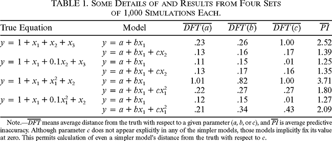
2. 2. These independent variables affect another variable, y, according to one of the four “true” equations shown in Table 1. These equations represent four types of situation. In the first, all of the independent variables have equally strong, linear effects on the dependent variable. In the second case, x ₂ has a weaker effect on y than either x ₁ or x ₃ does. In the third scenario, x ₃ does not affect y at all, and x ₁ has a nonlinear effect on y. The fourth scenario is the same as the third, except that x ₁ has a weaker nonlinear effect on y.

Table 1.Some Details of and Results from Four Sets of 1,000 Simulations Each.

True Equation	Model	$\overline{DFT\left(a\right)}$	$\overline{DFT\left(b\right)}$	$\overline{DFT\left(c\right)}$	$\overline{PI}$
$y=1+x_{1}+x_{2}+x_{3}$	$y=a+bx_{1}$	.23	.26	1.00	2.52
	$y=a+bx_{1}+cx_{2}$	.13	.16	.17	1.39
$y=1+x_{1}+0.1x_{2}+x_{3}$	$y=a+bx_{1}$	.11	.15	.01	1.25
	$y=a+bx_{1}+cx_{2}$	.13	.17	.16	1.35
$y=1+x_{1}+x^{2}_{1}+x_{2}$	$y=a+bx_{1}$	1.01	.82	1.00	3.71
	$y=a+bx_{1}+cx^{2}_{1}$	.22	.27	.27	1.80
$y=1+x_{1}+0.1x^{2}_{1}+x_{2}$	$y=a+bx_{1}$	.12	.15	.01	1.27
	$y=a+bx_{1}+cx^{2}_{1}$	.21	.34	.43	2.09

Note.—$\overline{DFT}$ means average distance from the truth with respect to a given parameter (a, b, or c), and$\overline{PI}$ is average predictive inaccuracy. Although parameter c does not appear explicitly in any of the simpler models, those models implicitly fix its value at zero. This permits calculation of even a simpler model's distance from the truth with respect to c.

Given the above “true” distributions, I randomly sampled a value of each independent variable x _i. Using these values, and one of the four “true” equations from Table 1, I calculated the value of the dependent variable y. I repeated this process 10 times, and then used the 10 resulting “data” to estimate parameter values for two models—a simpler one and a more complex one. In all cases, both of the models have fewer nonzero parameters than the stipulated full reality. This is meant to reflect the fact that models of even the simplest physical systems typically ignore at least some parameters associated with minor forces. Models of very complex systems must leave out even more.

Finally, I calculated two quantities:

1. 1. The distance from the truth about the model's parameter values (as defined in the previous section).

2. 2. The discrepancy (defined immediately below) between the prediction entailed by a given model, and a new randomly sampled data point, that is, a datum that was not among the 10 original data used to estimate that model's parameter values.

For each of the four scenarios corresponding to the four true equations, I repeated the above procedure 1,000 times. Table 1 presents some details and results of these simulations.

In terms of predictive accuracy, the more complex model has the advantage in the first and third scenarios. But the simpler model has the advantage in the second and fourth (Table 1). These latter scenarios are the kind of situation featured in Sober's argument for instrumentalism. In both, the more complex model comes closer to invoking the correct number of relevant nonzero parameters. But the simpler model nevertheless yields better predictions. Yet in all cases it is the model that, on average, is more accurate in terms of parameter values that has greater average predictive accuracy. As can be seen from Table 1, this match between average predictive inaccuracy and average distance from the truth occurs within every scenario and for every parameter.

A finer-grained look at the simulation results confirms this connection between predictive inaccuracy and distance from the truth. These two quantities covary positively among the individual simulations, just as they do when averaged over all 1,000 simulations as in Table 1. For every scenario, model, and applicable parameter,Footnote ⁵ there is a positive correlation (ranging from .04 to .89) between predictive success and verisimilitude.

These results justify the realist's inclination to interpret predictive success as evidence of approximate truth. And they support the realist's inference to verisimilitude as the best explanation of predictive success. As Hitchcock and Sober (Reference Hitchcock and Sober2004, 26) themselves put the miracle argument for scientific realism, “[W]hat else, besides the truth (or approximate truth) of theory T can be said to explain T's success in making novel predictions?”

5. Conclusion

Sober has gone beyond traditional arguments for instrumentalism. The most famous of these are the underdetermination of theory by evidence and the pessimistic induction. Both of these arguments provide good reason to doubt that many, if any, scientific theories achieve exact truth. But they cut no ice at all against the realist notion that scientists can and do use predictive success as a reliable guide for choosing theories that are closer than their competitors to that exact truth.

Sober has pointed out that one potential version of this realist notion is unsound. He has shown that in some cases of curve fitting, a theory achieves predictive superiority over its rivals, despite being less accurate than those rivals about the sheer number of nonzero parameters in the “true curve.” In this paper, I have demonstrated that even in such cases, predictive accuracy still tracks verisimilitude, but of a different kind, namely, accuracy about the values of parameters. This vindicates a sort of realism that posits this kind of accuracy, and not just predictive success for its own sake, as a goal of theory choice.