
1. Introduction
Richtmyer–Meshkov instability (RMI) occurs when a shock wave impacts on an interface between two fluids with different densities (Richtmyer Reference Richtmyer1960; Meshkov Reference Meshkov1969), and then induces finger-like flow structures such as the bubble (light fluid penetrating heavy one) and the spike (heavy fluid penetrating light one). It finally may cause a flow transition to turbulent mixing (Zhou et al. Reference Zhou, Clark, Clark, Glendinning, Skinner, Huntington, Hurricane, Dimits and Remington2019). Over the past decades, RMI has become a subject of intensive research due to its crucial role in various industrial and scientific fields such as inertial confinement fusion (ICF) (Lindl et al. Reference Lindl, Landen, Edwards, Moses and Team2014), supersonic combustion (Yang, Kubota & Zukoski Reference Yang, Kubota and Zukoski1993), supernova explosions (Kuranz et al. Reference Kuranz2018) and ejecta, material strength, chemical reactions, solar prominences and ionospheric flows (Zhou et al. Reference Zhou2021). The RMI on a semi-infinite single-mode interface that has the simplest mathematical form has been extensively studied (Brouillette Reference Brouillette2002; Zhou Reference Zhou2017a,Reference Zhoub; Zhai et al. Reference Zhai, Zou, Wu and Luo2018). However, RMI is generally involved in the issue of the multi-interface evolution. For example, RMI is initiated when the shocks generated by intense lasers or X-rays interact with the outer ablator layer, the middle push layer and the inner fuel layer of an ICF capsule. The mixing induced by RMI significantly reduces and even eliminates the thermonuclear yield. In addition, RMI occurs when the shocks generated by star collapse in a supernova interact with continuous multi-layer heavy elements throughout the interstellar space. The mixing induced by RMI shapes the filament structures in the supernova remnant. Therefore, it is significant to investigate the mixing caused by the RMI in a multi-interface system.
Most previous studies considered the RMI of an A/B/A-type fluid layer, i.e. two interfaces separating two kinds of fluids (gas A and gas B). Theoretically, the linear solutions for the amplitude growth rates of the two interfaces of an A/B/A-type fluid layer were separately derived by Jacobs et al. (Reference Jacobs, Jenkins, Klein and Benjamin1995) and Mikaelian (Reference Mikaelian1985, Reference Mikaelian1995, Reference Mikaelian1996). As the initial layer thickness reduces, the interface-coupling effect on the RMI is more prominent. Experimentally, the gas curtain technology was mainly adopted to explore the RMI of a thin SF $_6$ layer surrounded by air. It was found that the shock-induced morphologies of the SF
 $_6$ layer are sensitive to the initial shape of the layer (Jacobs et al. Reference Jacobs, Klein, Jenkins and Benjamin1993; Budzinski, Benjamin & Jacobs Reference Budzinski, Benjamin and Jacobs1994; Jacobs et al. Reference Jacobs, Jenkins, Klein and Benjamin1995; Rightley, Vorobieff & Benjamin Reference Rightley, Vorobieff and Benjamin1997), and the late-time mixing is influenced by initial conditions such as the perturbation amplitude and wavelength of the fluid layer, the incident shock strength, etc. (Prestridge et al. Reference Prestridge, Vorobieff, Rightley and Benjamin2000; Tomkins et al. Reference Tomkins, Kumar, Orlicz and Prestridge2008; Balakumar et al. Reference Balakumar, Orlicz, Tomkins and Prestridge2008; Orlicz et al. Reference Orlicz, Balakumar, Tomkins and Prestridge2009; Balakumar et al. Reference Balakumar, Orlicz, Ristorcelli, Balasubramanian, Prestridge and Tomkins2012; Orlicz, Balasubramanian & Prestridge Reference Orlicz, Balasubramanian and Prestridge2013; Tomkins et al. Reference Tomkins, Balakumar, Orlicz, Prestridge and Ristorcelli2013). The soap film technique was recently utilised to generate an SF
 $_6$ gas layer surrounded by air (Ding et al. Reference Ding, Li, Sun, Zhai and Luo2019; Liang et al. Reference Liang, Liu, Zhai, Si and Wen2020a; Li et al. Reference Li, Ding, Si and Luo2020; Sun et al. Reference Sun, Ding, Zhai, Si and Luo2020; Liang & Luo Reference Liang and Luo2021a,Reference Liang and Luob). It was determined that the waves reverberating inside a fluid layer induce various interfacial instabilities at the two sides of the fluid layer. For instance, the rarefaction waves inside an SF
 $_6$ layer impose the additional Rayleigh–Taylor instability (Rayleigh Reference Rayleigh1883; Taylor Reference Taylor1950) on the first interface, and the compression waves inside an SF
 $_6$ layer impose additional Rayleigh–Taylor stabilisation (RTS) on the second interface (Liang & Luo Reference Liang and Luo2021a). Differently, the reflected shocks reverberating inside a helium layer induce the additional RMI on the two interfaces (Liang & Luo Reference Liang and Luo2022).
On comparing with an A/B/A-type fluid layer, an A/B/C-type fluid layer, i.e. two interfaces separating three kinds of fluids (fluids A, B and C), is more general in its applications. For example, the double-shell ICF capsule consists of a CH form shell (35 mg ml $^{-1}$) between the outer shell (2.7 g ml
 $^{-1}$) and the inner shell (200 mg ml
 $^{-1}$) (Montgomery et al. Reference Montgomery2018; Haines et al. Reference Haines2021). The materials in various shells are entirely different. Moreover, the waves reverberating inside an A/B/C-type fluid layer are quite different from those inside an A/B/A-type fluid layer. As a result, it is expected that the influences of the reverberating waves on the two interfaces of a fluid layer are dissimilar under the A/B/C-type and A/B/A-type fluid-layer conditions. Moreover, designing an appropriate layer thickness could be used advantageously to minimise the mixing in ICF capsules (Drake Reference Drake2018). However, theoretical solutions and experiments on the RMI of an A/B/C-type fluid layer with variant layer thicknesses are still lacking.
In this work, we first derive a new linear model by considering the interface-coupling effect to evaluate the amplitude growth rates of the two interfaces of an A/B/C-type fluid layer in the weak-shock limit. Then, we extend the soap film technique to generate a fluid layer with two fast/slow interfaces, i.e. the fluid layer is located between a semi-infinite lighter gas and a semi-infinite heavier gas, which forms a light/medium/heavy (LMH) configuration. The lightest gas is air, the medium gas is a mixture of air and SF $_6$ (at moderate concentration) and the heaviest gas is a mixture of air and SF
 $_6$ (at high concentration). Later, we elaborate shock-tube experiments on three quasi-one-dimensional (quasi-1-D) LMH fluid layers with various layer thicknesses that are performed to investigate the wave patterns and interface motions. Further, shock-tube experiments on six quasi-two-dimensional (quasi-2-D) LMH fluid layers with different layer thickness and amplitude combinations are conducted to investigate the hydrodynamic instabilities of the two interfaces. Finally, the linear model is extended to a nonlinear one by considering the nonlinearity effect to describe the perturbation growths of the two interfaces in a later regime.
2. Linear stability analysis
We first perform a linear stability analysis to acquire the theoretical amplitude growth rates of the first interface ( $\dot {a}_1^l$) and the second interface (
 $\dot {a}_2^l$) of an A/B/C-type fluid layer by considering the interface-coupling effect. Different from the previous analysis on an A/B/A-type fluid layer (Jacobs et al. Reference Jacobs, Jenkins, Klein and Benjamin1995; Mikaelian Reference Mikaelian1996), we consider a more general system of three incompressible and initially irrotational fluids of densities
 $\rho _1$,
 $\rho _2$ and
 $\rho _3$, and velocity potentials
 $\phi _1$,
 $\phi _2$ and
 $\phi _3$, separated by two nearly planar interfaces with perturbations
 $\eta _1$ and
 $\eta _2$ and an initial layer thickness of
 $2h_0$, as sketched in figure 1.
Schematic showing the configuration analysed using linear stability theory for a more general system of three incompressible and initially irrotational fluids, where  $\rho _1$,
 $\rho _2$ and
 $\rho _3$ are the densities of the three fluids, and
 $\phi _1$,
 $\phi _2$ and
 $\phi _3$ are the velocity potentials;
 $\eta _1$ and
 $\eta _2$ are initial perturbations and
 $2h_0$ is the initial layer thickness.

The equations that govern the growth of infinitesimal disturbances on the boundaries of the layer are
 \begin{equation} \nabla^2\phi=0, \end{equation}
in each of the three fluids, with the kinematic conditions on  $y=\pm h_0$,
 \begin{equation} \frac{\partial\eta}{\partial t}-\frac{\partial\phi}{\partial y}=0, \end{equation}
and the conditions of the pressure equilibrium on  $y=\pm h_0$,
 \begin{equation} \rho\frac{\partial\phi}{\partial t}-\rho g\eta+p=P_0, \end{equation}
where  $p$ is pressure,
 $g$ is the acceleration and
 $P_0$ is a constant and equals the pressure at an unperturbed interface. Periodic perturbation amplitudes set on the first interface (
 $a_1$) and the second interface (
 $a_2$) are of the form
 \begin{equation} \eta_1=a_1(t)\cos(kx),\quad \eta_2=a_2(t)\cos(kx), \end{equation}
then requires the following velocity potentials in the three fluids (Jacobs et al. Reference Jacobs, Jenkins, Klein and Benjamin1995):
 \begin{equation} \left. \begin{aligned} & \phi_1=b_1(t)\mathrm{e}^{{-}k(y-h_0)}\cos(kx),\\ & \phi_2={-}\left[\frac{b_1+b_2}{2}\frac{\sinh(ky)}{\cosh(kh_0)}+\frac{b_1-b_2}{2}\frac{\cosh(ky)}{\sinh(kh_0)}\right]\cos(kx),\\ & \phi_3={-}b_2(t)\mathrm{e}^{k(y+h_0)}\cos(kx). \end{aligned} \right\} \end{equation}
Substituting (2.4a,b) and (2.5) into (2.2) and (2.3) yields
 \begin{gather} \frac{\mathrm{d}a_1}{\mathrm{d}t}={-}kb_1, \end{gather}
 \begin{gather} \frac{\mathrm{d}a_2}{\mathrm{d}t}={-}kb_2, \end{gather}
 \begin{gather} \left[\rho_1+\rho_2\tanh(kh_0)\right]\frac{\mathrm{d}b_1}{\mathrm{d}t}+\left[\rho_3+\rho_2\tanh(kh_0)\right]\frac{\mathrm{d}b_2}{\mathrm{d}t}=g\left[(\rho_1-\rho_2)a_1+(\rho_2-\rho_3)a_2\right], \end{gather}
 \begin{gather} \left[\rho_1+\rho_2\coth(kh_0)\right]\frac{\mathrm{d}b_1}{\mathrm{d}t}-\left[\rho_3+\rho_2\coth(kh_0)\right]\frac{\mathrm{d}b_2}{\mathrm{d}t}=g\left[(\rho_1-\rho_2)a_1+(\rho_3-\rho_2)a_2\right]. \end{gather}
Equations (2.6)–(2.9) can be combined to yield a pair of ordinary differential equations for  $a_1$ and
 $a_2$
 \begin{gather} \left[\rho_1+\rho_2\tanh(kh_0)\right]\frac{\mathrm{d}^2a_1}{\mathrm{d}t^2}+\left[\rho_3+\rho_2\tanh(kh_0)\right]\frac{\mathrm{d}^2a_2}{\mathrm{d}t^2}= kg\left[(\rho_2-\rho_1)a_1+(\rho_3-\rho_2)a_2\right], \end{gather}
 \begin{gather} \left[\rho_1+\rho_2\coth(kh_0)\right]\frac{\mathrm{d}^2a_1}{\mathrm{d}t^2}-\left[\rho_3+\rho_2\coth(kh_0)\right]\frac{\mathrm{d}^2a_2}{\mathrm{d}t^2}=kg\left[(\rho_2-\rho_1)a_1+(\rho_2-\rho_3)a_2\right]. \end{gather}
For RMI, the acceleration  $g$ can be replaced by the jump speed of a fluid layer (
 $\Delta v$) and a Dirac delta function (i.e.
 $g=\Delta v\delta t$ with
 $\delta t=0$ when
 $t=0$ and
 $\delta t=1$ when
 $t>0$) allowing (2.10) and (2.11) to be easily integrated in the weak-shock limit. Thus,
 \begin{align} &\left[\rho_1+\rho_2\tanh(kh_0)\right]\dot{a}_1^l+\left[\rho_3+\rho_2\tanh(kh_0)\right]\dot{a}_2^l\nonumber\\ &\quad =k\Delta v\left[(\rho_2-\rho_1)a_1(0)+(\rho_3-\rho_2)a_2(0)\right], \end{align}
 \begin{align} &\left[\rho_1+\rho_2\coth(kh_0)\right]\dot{a}_1^l-\left[\rho_3+\rho_2\coth(kh_0)\right]\dot{a}_2^l\nonumber\\ &\quad =k\Delta v\left[(\rho_2-\rho_1)a_1(0)+(\rho_2-\rho_3)a_2(0)\right]. \end{align}
There are a few linear models considering different post-shock parameter combinations to evaluate the compression effect induced by the incident shock (Richtmyer Reference Richtmyer1960; Meyer & Blewett Reference Meyer and Blewett1972; Fraley Reference Fraley1986; Vandenboomgaerde, Mügler & Gauthier Reference Vandenboomgaerde, Mügler and Gauthier1998). In this study, we shall follow the original prescriptions introduced by Richtmyer (Reference Richtmyer1960) since the Richtmyer model has the most simplified form sufficient to quantify the linear amplitude growth rate of a fast/slow interface in the weak-shock limit. Replacing the pre-shock parameters in (2.12) and (2.13) with the post-shock parameters of the two interfaces,  $\dot {a}_1^l$ and
 $\dot {a}_2^l$ can be separately solved as
 \begin{gather} \dot{a}_1^l={-}\frac{k\Delta v_1 Z_1a_1(0)\left[(R_1-1)(2R_3\xi+\xi^2+1)+(1-R_3)(1-\xi^2)/\epsilon\right]}{2\xi(R_1R_3+1)+(R_1+R_3)(\xi^2+1)}, \end{gather}
 \begin{gather} \dot{a}_2^l=\frac{k\Delta v_2 Z_2a_2(0)\left[\epsilon(R_1-1)(\xi^2-1)-(1-R_3)(2R_1\xi+\xi^2+1)\right]}{2\xi(R_1R_3+1)+(R_1+R_3)(\xi^2+1)}, \end{gather}
in which  $\Delta v_1$ denotes the velocity jump of the first interface induced by the incident shock (IS),
 $\Delta v_2$ denotes the velocity jump of the second interface induced by the transmitted shock inside the fluid layer (TS
 $_1$);
 $Z_1$ (
 $=1-\Delta v_1/v_{{IS}}$) and
 $Z_2$ (
 $=1-\Delta v_1/v_{{TS_1}}$) are compression factors with
 $v_{{IS}}$ and
 $v_{{TS_1}}$ denoting the speed of the IS and the TS
 $_1$, respectively;
 $\xi =\tanh (Z_Lkh_0)$,
 $Z_L=1-\Delta v_1/v_{{TS_1}}$,
 $R_1=\rho _1/\rho _2$,
 $R_3=\rho _3/\rho _2$ and
 $\epsilon =Z_1a_1(0)/Z_2a_2(0)$. Here, (2.14) and (2.15) are called the LL model. Notably, the LL model is also applicable to an A/B/A-type fluid layer when
 $R_1=R_3$.
3. Experimental method
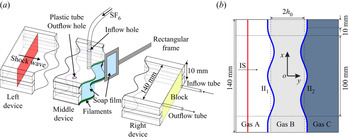
The soap film technique is extended to generate two shape-controllable and discontinuous interfaces of an LMH fluid layer, mainly eliminating the additional short-wavelength perturbations, diffusion layer and three-dimensionality (Liu et al. Reference Liu, Liang, Ding, Liu and Luo2018; Liang et al. Reference Liang, Zhai, Ding and Luo2019; Luo et al. Reference Luo, Liu, Liang, Ding and Wen2020; Liang et al. Reference Liang, Liu, Zhai, Ding, Si and Luo2021). As shown in figure 2(a), three transparent devices (i.e. left device, middle device and right device) with a width of 140.0 mm and a height of 10.0 mm are first manufactured using transparent acrylic sheets with a thickness of 3.0 mm. The middle device's adjacent boundaries are carefully engraved to be of a sinusoidal shape with a depth of 1.8 mm. Then, four thin filaments (marked green in figure 2a) with a height of 2.0 mm are attached to the upper and lower plates’ inner surfaces at two sides of the middle device to restrict the soap film's shape. Thus the filament bulges in the flow field with only 0.2 mm height. Before the interface formation, the filaments are properly wetted by a soap solution with a mass fraction of 78 % distilled water, 2 % sodium oleate and 20 % glycerine.
Schematics of (a) the soap film interface generation and (b) the initial configuration studied in the present work, where  $h_0$ denotes half of the initial layer thickness, II
 $_1$ denotes the first initial interface and II
 $_2$ denotes the second initial interface.

First, a small rectangular frame with moderate soap solutions dipped on its borders is pulled along the sinusoidal filaments on both sides of the middle device. Two soap film interfaces are formed, and the middle device is closed. Second, SF $_6$ is pumped into the closed space through an inflow hole to discharge air inside through an outflow hole. An oxygen concentration detector is placed at the outflow hole to monitor the concentration of SF
 $_6$ inside the closed space. Third, when the volume fraction of oxygen at the outflow hole reduces to 10 %, both the inflow and outflow holes are sealed. Fourth, the left and right transparent devices are gently connected to the middle device, and the combined one is inserted into the open-ended test section of a shock tube. Fifth, the end of the right device is sealed with a block. Then, SF
 $_6$ is injected into the right device through an inflow tube at the right bottom corner of the block, and the air is exhausted through an outflow tube at the left top corner of the block. In the meantime, the oxygen concentration detector is placed at the end of the outflow tube to monitor the concentration of SF
 $_6$ inside the right device. Sixth, the inflow and outflow tubes are sealed when the detected oxygen concentration decreases to around 0.02 %. Finally, shock-tube experiments are conducted as soon as possible to reduce gas diffusion among the various devices.
In the Cartesian coordinate system, as sketched in figure 2(b), the initial perturbations on the  $n$th interface are single mode as
 $y=a_{n}(0)\cos (kx+{\rm \pi} )$ within the range of
 $x\in [-60.0,60.0]\,\mathrm {mm}$, where
 $k$ denotes the wavenumber of the two interfaces. In this work,
 $k=104.7$ m
 $^{-1}$;
 $a_{1}(0)$ and
 $a_{2}(0)$ in all cases are listed in table 1. To minimise the wall effect of the shock tube on the interface evolution, a short flat part with 10.0 mm on each side of the two interfaces is adopted. Its influence on the interface evolution is limited (Luo et al. Reference Luo, Liang, Si and Zhai2019). The initial layer thickness (
 $2h_0$) is defined as the distance between the average positions of the first initial interface (II
 $_1$) and the second initial interface (II
 $_2$). Overall, we shall investigate three quasi-1-D LMH fluid layers with no perturbations and six quasi-2-D LMH fluid layers with three initial layer thicknesses and two amplitude combinations. Here, we define the three cases (i.e. cases L10-IP, L30-IP and L50-IP) with
 $a_2(0)>0$ as in-phase cases and the three cases (i.e. cases L10-AP, L30-AP and L50-AP) with
 $a_2(0)<0$ as anti-phase cases. As sketched in figure 2(b), gas A (light gas) is air, gas B (medium gas) is a mixture of air and SF
 $_6$ (with a moderate mass fraction
 $MF_B$) and gas C (heavy gas) is a mixture of air and SF
 $_6$ (with a high mass fraction
 $MF_C$). The Atwood number of the first interface is
 $A_1$ (
 $=(\rho _B-\rho _A)/(\rho _B+\rho _A)$, with
 $\rho _A$ denoting the density of gas A and
 $\rho _B$ denoting the density of gas B), and the Atwood number of the second interface is
 $A_2$ (
 $=(\rho _C-\rho _B)/(\rho _C+\rho _B)$, with
 $\rho _C$ denoting the density of gas C), respectively. The values of
 $MF_B$,
 $MF_C$,
 $A_1$ and
 $A_2$ are listed in table 1.
Physical parameters of a LMH fluid layer, where  $a_{1}(0)$ (
 $a_{2}(0)$) denotes the initial amplitude of the first (second) interface,
 $h_0$ denotes half of the initial layer thickness,
 $MF_B$ (
 $MF_C$) denotes the mass fraction of SF
 $_6$ in gas B (gas C) and
 $A_1$ (
 $A_2$) denotes the Atwood number of the first (second) initial interface.

The ambient pressure and temperature are 101.3 kPa and  $295.5\pm 1.0$ K, respectively. The IS with a Mach number of
 $1.20\pm 0.01$ travels from left to right. The value of
 $v_{{IS}}$ is
 $414\pm 1$ m s
 $^{-1}$. The flow field is monitored by high-speed Schlieren photography. The frame rate of the high-speed video camera (FASTCAM SA5, Photron Limited) is 60 000 f.p.s. and the shutter time is 1
 $\mathrm {\mu }$s. The spatial resolution of the Schlieren images is 0.4 mm pixel
 $^{-1}$. The flow field visualisation is limited within the range of
 $x\in [-50.0,50.0]\,\mathrm {mm}$, as shown in figure 2(b).
4. Quasi-1-D experimental results and analysis
We shall first describe the reverberating waves observed from Schlieren images. Then, the interface displacements and velocities are measured and compared among different layer-thickness cases. Last, the speeds of the two interfaces after they are affected by the reverberating waves are deduced. In this way, a general 1-D theory for describing the interface motion is established.
4.1. Experimental observation
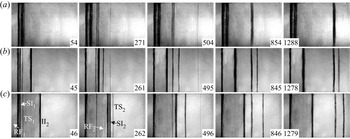
Schlieren images of the shock-induced quasi-1-D LMH fluid-layer evolution are shown in figure 3(a–c) for  $2h_0=10.0$, 30.0 and 50.0 mm, respectively. The moment when the IS impacts the average position of the first initial interface (II
 $_1$) is defined as
 $t=0$. Taking the L50-1D case as an example, the wave patterns and interface motions are discussed in detail. After the IS impacts the II
 $_1$, the reflected shock (RF
 $_1$) and the transmitted shock (TS
 $_1$) are immediately generated, and the shocked first interface (SI
 $_1$) begins to move forwards (46
 $\mathrm {\mu }$s). Then, the TS
 $_1$ impacts the second initial interface (II
 $_2$), and a transmitted shock (TS
 $_2$) is refracted outside the fluid layer and followed by the shocked second interface (SI
 $_2$) (262
 $\mathrm {\mu }$s). Meanwhile, a weak shock wave (RF
 $_2$) is reflected inside the fluid layer since the SI
 $_2$ is a fast/slow interface relative to the motion of the TS
 $_1$. Theoretically, after the RF
 $_2$ impacts the SI
 $_1$, rarefaction waves (RW) should be reflected inside the fluid layer since the SI
 $_1$ is a slow/fast interface relative to the motion of the RF
 $_2$. However, due to the RW's limited strength, the density variation induced by the RW is restricted, and it is challenging to distinguish the RW. Finally, all waves are refracted outside the fluid layer, and the interfaces at the two sides of the fluid layer move at the same speed. Moreover, it is noted that the two interfaces coalesce to one at a late time when the initial layer is very thin (1288
 $\mathrm {\mu }$s in the L10-1D case).
Schlieren images of the shock-induced quasi-1-D LMH fluid-layer evolution in cases (a) L10-1D, (b) L30-1D and (c) L50-1D, where SI $_1$ (SI
 $_2$) denotes the shocked first (second) interface, RF
 $_1$ (TS
 $_1$) denotes the reflected (transmitted) shock after the IS impacts II
 $_1$ and RF
 $_2$ (TS
 $_2$) denotes the reflected (transmitted) shock after the TS
 $_1$ impacts II
 $_2$. Numbers indicate time in
 $\mathrm {\mu }$s.

The displacements ( $y_{{SI}_n}$) and velocities (
 $v_{{SI}_n}$) of the two interfaces are measured from experiments (
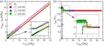
 $n=1$ for the first interface and 2 for the second interface), and are shown in figures 4(a) and 4(b), respectively. The pixel size of the Schlieren images introduces the experimental measurement uncertainty and is 0.4 mm in this work. The size of the error bars equals the size of the symbols in the figures. Time is scaled as
 $tv_{{TS_1}}/(2h_0)$, interface displacement is scaled as
 $(y_{{SI}_n}-y_{01})/(2h_0)$, with
 $y_{01}$ denoting the initial position of the first interface, and interface velocity is scaled as
 $v_{{SI}_n}/\Delta v_{1}$. The values of
 $v_{{TS_1}}$ and
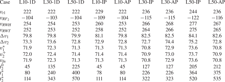
 $\Delta v_{1}$ in all cases are calculated according to the 1-D gas dynamics theory (Drake Reference Drake2018), as listed in table 2. The dimensionless displacements and velocities of the first (second) interface converge in all
 $h_0$ cases, as shown in figure 4(a,b), which indicates that the dimensionless movements of the two interfaces are independent of the initial layer thickness.
The dimensionless displacements (a) and velocities (b) of the first interface (solid symbols) and the second interface (hollow symbols). Black and orange solid lines represent the 1-D theory predictions for the first interface motions in Stages I ( $t_{1}^{*}>t>0$) and II (
 $t>t_{1}^{*}$), respectively. Black and purple dashed lines represent the 1-D theory predictions for the second interface motions in Stages I (
 $t_{2}^{*}>t>t_{2}^{0}$) and III (
 $t>t_{2}^{+}$), respectively.

Physical parameters of the waves and interfaces of an LMH fluid layer in the laboratory reference, where  $v_{{TS_1}}$ denotes the speed of the TS
 $_1$,
 $v_{{RF}_2}$ denotes the speed of the RF
 $_2$,
 $v_{{RWH}}$ denotes the speed of the RWH,
 $v_{{RWT}}$ denotes the speed of the RWT,
 $\Delta v_{1}$ (
 $\Delta v_{2}$) denotes the speed of the SI
 $_1$ (SI
 $_2$) in Stage I,
 $v_{1}^*$ denotes the speed of the SI
 $_1$ in Stage II,
 $v_{2}^+$ denotes the speed of the SI
 $_2$ in Stage III,
 $v_{fn}$ denotes the asymptotic velocity of the two interfaces,
 $t_{2}^0$ denotes the specific time when the TS
 $_2$ impacts II
 $_2$,
 $t_{1}^*$ denotes the specific time when the RF
 $_2$ impacts SI
 $_1$ and
 $t_{2}^*$ denotes the specific time when the RWH impacts SI
 $_2$. RWT denotes the rarefaction wave tail. The units for speed and time are m s
 $^{-1}$ and
 $\mathrm {\mu }$s, respectively.

4.2. Characteristics of reverberating waves
The waves reverberating inside an LMH fluid layer are sketched in figure 5(a–d). To have a clear description of the interaction of a reverberating wave and interface, we first define several specific times including  $t_2^0$ when the TS
 $_1$ impacts the II
 $_2$,
 $t_1^*$ when the RF
 $_2$ impacts the SI
 $_1$ and
 $t_2^*$ when the rarefaction wave head (RWH) impacts the SI
 $_2$. Then
 $t_2^0$,
 $t_1^*$ and
 $t_2^*$ can be evaluated as
 \begin{equation} \left. \begin{aligned} & t_2^0=\frac{2h_0}{v_{{TS_1}}},\\ & t_1^*=t_2^0+\frac{2h_0-t_2^0\Delta v_1}{\Delta v_1-v_{{RF}_2}},\\ & t_2^*=t_1^*+\frac{2h_0-t_2^0\Delta vv_1+(t_1^*-t_2^*)(\Delta v_2-\Delta v_1)}{v_{{RWH}}-\Delta v_2}, \end{aligned} \right\} \end{equation}
in which  $v_{{RF}_2}$ represents the speed of the RF
 $_2$,
 $v_{{RWH}}$ represents the speed of the RWH. The values of
 $v_{{RF}_2}$,
 $v_{{RWH}}$ and
 $\Delta v_2$ are calculated according to the 1-D gas dynamics theory (Drake Reference Drake2018), and then
 $t_2^0$,
 $t_1^*$ and
 $t_2^*$ are obtained, as listed in table 2.
Sketches of (a) the interaction of the TS $_1$ and II
 $_2$ at
 $t_2^0$, (b) the interaction of the RF
 $_2$ and SI
 $_1$ at
 $t_1^*$, (c) the interaction of the RW and SI
 $_2$ at
 $t_2^*$ and (d) the motions of the SI
 $_1$ and SI
 $_2$ when
 $t>t_2^+$.

After the RF $_2$ impacts the SI
 $_1$, the speed of the SI
 $_1$ decreases from
 $\Delta v_1$ to
 $v_1^*$. The values of
 $v_1^*$ can be calculated according to the 1-D gas dynamics theory (Drake Reference Drake2018), as listed in table 2. After the RW impact the SI
 $_2$, the speed of the SI
 $_2$ reduces from
 $v_2^\alpha$ to
 $v_2^+$. The interaction of the RW and a fast/slow interface (i.e. SI
 $_2$) is different from the interaction of the RW and a slow/fast interface previously investigated (Liang & Luo Reference Liang and Luo2021a). Based on the 1-D gas dynamics theory (Velikovich & Phillips Reference Velikovich and Phillips1996; Drake Reference Drake2018),
 $v_2^+$ can be calculated as
 \begin{equation} v_2^+{=}\Delta v_2+\frac{2c_5}{\gamma_5-1}[p_{31}^{(\gamma_5-1)/2\gamma_5}-1], \end{equation}
where  $\gamma _5$ is the specific heat ratio of gas C,
 $c_5$ is the sound speed of gas C after the TS
 $_1$ impacts the II
 $_2$. The only unknown parameter
 $p_{31}$, i.e. the ratio of the pressure of the flow after the RWT leaves the SI
 $_2$ (
 $p_3$) to the pressure of the flow between the RF
 $_2$ and SI
 $_2$ (
 $p_1$), as sketched in figure 5(b,d), satisfies
 \begin{equation}
\frac{c_5}{c_1}=\frac{(\gamma_5-1)[p_{31}^{(\gamma_1-1)/2\gamma_1}-2p_{21}^{(\gamma_1-1)/2\gamma_1}+1]}{(\gamma_1-1)[1-p_{31}^{(\gamma_5-1)/2\gamma_5}]},
\end{equation}
where  $\gamma _1$ is the specific heat ratio of gas B,
 $c_1$ is the sound speed of gas B after the TS
 $_1$ impacts the II
 $_2$ and
 $p_{21}$ is the ratio of the pressure of the flow between the RWT and SI
 $_1$ (
 $p_2$) to
 $p_1$. Then the
 $v_2^+$ can be calculated by solving (4.2)–(4.3), as listed in table 2.
The number of reverberating waves is infinite. However, the consecutive changes of pressure and velocity imparted by these reverberations decrease continuously, eventually converging to a well-defined asymptotic 1-D post-shock state. The influences of the reverberating waves on the 1-D and 2-D dynamics of the two interfaces should be considered (Aglitskiy et al. Reference Aglitskiy2006) until the two interfaces enter the asymptotic post-shock state. A simple and advantageous method is adopted to judge whether the higher-order reverberations should be accounted for or not. The interaction of an IS with a semi-infinite interface separating two fluids with  $\rho _1$ and
 $\rho _3$ is considered, and the intermediate layer is ignored. Then, the final post-shock velocity,
 $v_{{fn}}$, can be calculated according to the 1-D gas dynamics theory (Drake Reference Drake2018). As listed in table 2, the asymptotic velocity
 $v_{{fn}}$ is the same as
 $v_1^*$ and is 0.1 % smaller than
 $v_2^+$. Therefore, it is reasonable to regard that, after the RWT leaves the SI
 $_2$, the motions of the two interfaces enter the asymptotic state. Unlike the sudden acceleration imposed by a shock wave on an interface, the interaction of the RW and an interface is generally regarded as a continuous process (Li & Book Reference Li and Book1991; Li, Kailasanath & Book Reference Li, Kailasanath and Book1991; Morgan, Likhachev & Jacobs Reference Morgan, Likhachev and Jacobs2016; Morgan et al. Reference Morgan, Cabot, Greenough and Jacobs2018; Liang et al. Reference Liang, Zhai, Luo and Wen2020b; Liang & Luo Reference Liang and Luo2021a). The length of the RW (
 $L_{RW}$), the interaction time of the RW with SI
 $_2$ (
 $T_{{RW}}$) and the average deceleration imposed on the SI
 $_2$ by the RW (
 $\bar {g}_{{RW}}$) are separately deduced as
 \begin{equation} \left. \begin{aligned} & L_{RW}=(v_{{RWH}}-v_{{RWT}})(t_2^*-t_1^*),\\ & T_{{RW}}=\frac{2L_{RW}}{2u_{{RWT}}-\Delta v_2-v_2^+},\\ & \bar{g}_{{RW}}=\frac{v_2^+{-}\Delta v_2}{T_{{RW}}}, \end{aligned} \right\} \end{equation}
where  $u_{{RWT}}$ denotes the speed of the RWT. The values of
 $L_{RW}$,
 $T_{{RW}}$ and
 $\bar {g}_{{RW}}$ in all cases are calculated according to (4.4), as listed in table 3. As the layer thickness increases, both the
 $L_{RW}$ and
 $T_{{RW}}$ increase, whereas the
 $|\bar {g}_{{RW}}|$ decreases.
Physical parameters of the RW inside an LMH fluid layer. Here,  $L_{{RW}}$ denotes the length of the RW at
 $t_2^*$;
 $T_{{RW}}$ denotes the interaction time of the RW and SI
 $_2$, and
 $\bar {g}_{{RW}}$ denotes the average deceleration imposed on the SI
 $_2$ by the RW. The units for length, time and deceleration are mm,
 $\mathrm {\mu }$s and
 $10^6\times$ m s
 $^{-2}$, respectively.

It is evident that the motions of the two interfaces of a shocked LMH fluid layer can be divided into several stages, as illustrated in figure 4(b). Specifically, the first interface's motion can be separated into two stages: Stage I. Uniform motion with the  $\Delta v_1$ during
 $t_1^*>t>0$; Stage II. Uniform motion with the
 $v_1^*$ during
 $t>t_1^*$. The second interface's motion can be divided into three stages: Stage I. Uniform motion with the
 $\Delta v_2$ during
 $t_2^*>t>t_2^0$; Stage II. Deceleration with the
 $\bar {g}_{{RW}}$ during
 $t_2^+>t>t_2^*$ with
 $t_2^+=t_2^*+T_{{RW}}$; Stage III. Uniform motion with the
 $v_2^+$ during
 $t>t_2^+$. In fact, the motions of the two interfaces can be described by the derived specific times (4.1) and interface velocities ((4.2)–(4.4)), which actually form a general 1-D theory for the interface motion. The predictions of the 1-D theory for the first interface motions in Stages I and II are marked with black and orange solid lines in figure 4(a,b), and they agree well with the experimental results. The predictions of the 1-D theory for the second interface motions in Stages I and III are marked as black and purple dashed lines, and they agree well with the experimental results. Due to the limited duration of Stage II for the second interface (e.g.
 $T_{{RW}}$ is only around 1
 $\mathrm {\mu }$s in this study), the second interface motions in Stage II are not represented in figure 4(a,b).
5. Quasi-2-D experimental results and analysis
We shall first describe the deformations of the two interfaces observed from Schlieren images. Then, the amplitude growth rates are acquired from experiments and compared with the predictions of the LL model. Later, the interface-coupling effect on the RMI of the two interfaces is quantified and discussed. Last, the influences of the reverberating waves and the nonlinearity on the hydrodynamic instabilities of the two interfaces are modelled.
5.1. Experimental results
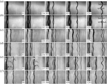
Schlieren images of the shock-induced quasi-2-D LMH fluid-layer evolution are shown in figure 6(a–f). Taking the L50-IP case as an example, the deformations of the two interfaces are discussed in detail. After the IS impacts the perturbed II $_1$, the rippled RF
 $_1$ is reflected outside the fluid layer, and the rippled TS
 $_1$ moves towards the II
 $_2$ (53
 $\mathrm {\mu }$s). Meanwhile, the perturbation on the SI
 $_1$ increases due to the vorticity deposited by the IS on the SI
 $_1$. After the TS
 $_1$ impacts the perturbed II
 $_2$, the rippled TS
 $_2$ is refracted outside the fluid layer, and the rippled RF
 $_2$ is reflected inside the fluid layer. Meanwhile, the perturbation on the SI
 $_2$ increases due to the vorticity deposited by the TS
 $_1$ on the SI
 $_2$ (237
 $\mathrm {\mu }$s). Finally, all waves are refracted outside the fluid layer, and the two interfaces evolve with the same phase as their initial perturbations. In addition, different from the large
 $h_0$ cases, portions of the two interfaces collide when
 $h_0$ is limited. For example, bubbles of the two interfaces collide at 1284
 $\mathrm {\mu }$s in the L10-IP case, and the bubble of the SI
 $_1$ collides with the spike of the SI
 $_2$ at 509
 $\mathrm {\mu }$s in the L10-AP case.
Schlieren images of the shock-induced quasi-2-D LMH fluid-layer evolution in cases (a) L10-IP, (b) L10-AP, (c) L30-IP, (d) L30-AP, (e) L50-IP and ( f) L50-AP. Here, ‘bub’ and ‘spi’ denote bubble and spike, respectively. Numbers denote time in  $\mathrm {\mu }$s.

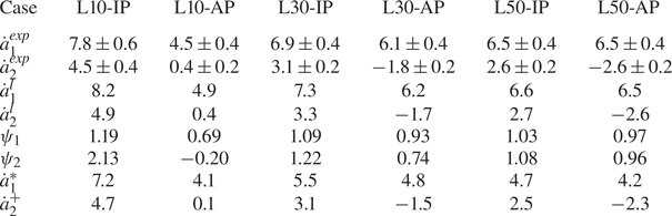
The experimental amplitude growth rate of the first interface ( $\dot {a}_1^{{exp}}$) and that of the second interface (
 $\dot {a}_2^{{exp}}$) in Stage I are acquired by linearly fitting the experimental data, as listed in table 4. In the three in-phase cases, as
 $h_0$ decreases, both
 $v_1^{{exp}}$ and
 $\dot {a}_2^{{exp}}$ increase. However, in the three anti-phase cases, as
 $h_0$ decreases, both
 $\dot {a}_1^{{exp}}$ and
 $|\dot {a}_2^{{exp}}|$ decrease. The results indicate that the RMI of an LMH fluid layer is influenced by the initial layer thickness and phases of the two interfaces, i.e. the interface-coupling effect. Due to the interface-coupling effect on the RMI of the second interface in the L10-AP case, an opposite sign of the amplitude growth rate of a fast/slow interface to its initial perturbation amplitude is observed. For a semi-infinite fast/slow Richtmyer–Meshkov (RM) unstable interface, the sign of its amplitude growth rate should be the same as the sign of its initial amplitude (Richtmyer Reference Richtmyer1960). In general, the amplitude growth rate of a semi-infinite slow/fast RM unstable interface has the opposite sign to its initial amplitude, which is ascribed to the phase reversal (Brouillette Reference Brouillette2002). The phase reversal of a shocked fast/slow interface (the second interface in the L10-AP case) is called ‘abnormal phase reversal’ in this study.
The linear amplitude growth rates of the two interfaces of an LMH fluid layer, where  $\dot {a}_1^{{exp}}$ (
 $\dot {a}_2^{{exp}}$) denotes the experimental amplitude growth rate of the first (second) interface in Stage I,
 $\dot {a}_1^l$ (
 $\dot {a}_2^l$) denotes the amplitude growth rate of the first (second) interface in Stage I calculated with (2.14) (2.15);
 $\psi _1$ (
 $\psi _2$) quantifies the interface-coupling effect on the RMI of the first (second) interface calculated with (5.1);
 $\dot {a}_1^{{*}}$ denotes the amplitude growth rate of the first interface at
 $t_1^*$ calculated with (5.2) and
 $\dot {a}_2^{{+}}$ denotes the amplitude growth rate of the second interface at
 $t_2^+$ calculated with (5.4)–(5.6).

The values of  $\dot {a}_1^l$ and
 $\dot {a}_2^l$ are calculated with the LL model and listed in table 4, and a good agreement with the experimental results is found. It is noted that
 $\dot {a}_2^l$ also has the opposite sign to
 $a_2(0)$ in the L10-AP case.
5.2. The interface-coupling effect
To quantify the interface-coupling effect on the RMI of an arbitrary fluid layer, we first propose a normalised growth rate ( $\psi _n$) which is defined as the ratio of the amplitude growth rate of the
 $n$th interface calculated with the LL model to that calculated with the impulsive theory (Richtmyer Reference Richtmyer1960),
 \begin{equation} \left. \begin{aligned} & \psi_1=\frac{(R_1+1)(2R_3\xi+\xi^2+1)-(R_1+1)(R_3-1)(1-\xi^2)/[\epsilon(R_1-1)]}{2\xi(R_1R_3+1)+(R_1+R_3)(\xi^2+1)},\\ & \psi_2=\frac{\epsilon(R_1-1)(R_3+1)(\xi^2-1)/(R_3-1)+(R_3+1)(2R_1\xi+\xi^2+1)}{2\xi(R_1R_3+1)+(R_1+R_3)(\xi^2+1)}. \end{aligned} \right\} \end{equation}
The values of  $\psi _1$ and
 $\psi _2$ in all the LMH layer cases are listed in table 4. It is found that
 $\psi _1>1$ and
 $\psi _2>1$ in the three in-phase cases, and
 $\psi _1<1$ and
 $|\psi _2|<1$ in the three anti-phase cases, indicating that the interface-coupling effect leads to the two in-phase interfaces being more unstable than the semi-infinite RMI, and the two anti-phase interfaces being more stable than the semi-infinite RMI, under the LMH fluid-layer condition. The conclusion is opposite to the A/B/A-type fluid-layer counterpart, i.e. the interface-coupling effect results in the two in-phase interfaces of an A/B/A-type fluid layer being more stable, and the two anti-phase interfaces being more unstable (Liang & Luo Reference Liang and Luo2021a, Reference Liang and Luo2022).
It is proved that the interface-coupling effect is determined by the density ratios of the fluids outside the layer to the fluid inside the layer ( $R_1$ and
 $R_3$), the post-shock amplitude ratio of the two interfaces (
 $\epsilon$) and the dimensionless post-shock layer thickness (
 $Z_Lkh_0$). The values of
 $\psi _{n}$ of an LMH fluid layer vs
 $Z_Lkh_0$ under different
 $R_1$,
 $R_3$ and
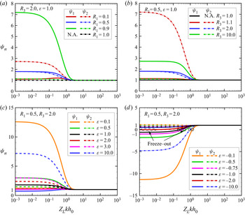
 $\epsilon$ conditions are calculated based on (5.1), as shown in figure 7(a–d), respectively.
Value of  $\psi _{n}$ of the
 $n$th interface vs
 $Z_Lkh_0$ under (a) different
 $R_1$ conditions, (b) different
 $R_3$ conditions, (c) different
 $\epsilon$ (
 $>0$) conditions and (d) different
 $\epsilon$ (
 $<0$) conditions. Hollow circles represent the instability freeze out of the first or second interface.

In figure 7(a), we plot  $\psi _1$ and
 $\psi _2$ as functions of
 $Z_Lkh_0$ for the case
 $R_1$ varying from 0.1 to 1.0,
 $R_3=2.0$ and
 $\epsilon =1.0$. When
 $Z_Lkh_0<2$,
 $\psi _1>1$ and
 $\psi _2>1$ indicate that the interface-coupling effect results in the two interfaces of an LMH fluid layer being more unstable if the two interfaces are initially in phase. Specifically, when
 $R_1\leq (1/R_3)$ (
 $R_1>(1/R_3)$),
 $\psi _1\leq \psi _2$ (
 $\psi _1>\psi _2$), indicating the interface-coupling effect destabilises the second interface more (less) than the first interface. When
 $Z_Lkh_0>2$,
 $\psi _1$ and
 $\psi _2$ converge at 1, revealing that the interface-coupling effect has a negligible influence on the RMI of a fluid layer.
In figure 7(b), we plot  $\psi _1$ and
 $\psi _2$ as functions of
 $Z_Lkh_0$ for the case
 $R_3$ varying from 1.0 to 10.0,
 $R_1=0.5$ and
 $\epsilon =1.0$. It is found that, when
 $R_3\leq (1/R_1)$ (
 $R_3>(1/R_1)$),
 $\psi _1\leq \psi _2$ (
 $\psi _1>\psi _2$), indicating the interface-coupling effect destabilises the second interface more (less) than the first interface, which agrees well with the findings in figure 7(a).
In figure 7(c), we plot  $\psi _1$ and
 $\psi _2$ as functions of
 $Z_Lkh_0$ for the case
 $\epsilon$ varying from 0.1 to 10.0,
 $R_1=0.5$ and
 $R_3=2.0$. It is found that when
 $3.0>\epsilon >0$,
 $\psi _1>1$ and
 $\psi _2>1$, indicating that the interface-coupling effect results in both interfaces being more unstable. Specifically, the interface-coupling effect promotes the RMI of the first interface more than the second interface counterpart (i.e.
 $\psi _1>\psi _2$) when
 $1.0>\epsilon >0$, and the interface-coupling effect promotes the RMI of the second interface more than the first interface counterpart (i.e.
 $\psi _1<\psi _2$) when
 $3.0>\epsilon >1.0$. In addition, when
 $\epsilon >3.0$,
 $\psi _1<1$ and
 $\psi _2>1$, demonstrating that the interface-coupling effect leads to the first interface being more stable, and the second interface being more unstable. Overall, the two in-phase interfaces of an LMH fluid layer are generally destabilised by the interface-coupling effect, but the first interface might be stabilised if the
 $\epsilon$ is large.
In figure 7(d), we plot  $\psi _1$ and
 $\psi _2$ as functions of
 $Z_Lkh_0$ for the case
 $\epsilon$ varying from
 $-$0.1 to
 $-$10.0,
 $R_1=0.5$ and
 $R_3=2.0$. It is found that, when
 $0>\epsilon >-2.0$ and
 $Z_Lkh_0<2$,
 $\psi _1<0$ and
 $\psi _2>0$, indicating that the interface-coupling effect results in the abnormal phase reversal of the first interface. The interface-coupling effect leads to the first interface being more unstable when
 $0>\epsilon >-0.75$ and the second interface being more stable when
 $0>\epsilon >-0.5$. When
 $\epsilon <-2.0$,
 $1>\psi _1>0$ and
 $\psi _2<0$, demonstrating that the interface-coupling effect causes the first interface to be more stable, and abnormal phase reversal of the second interface. Moreover, the instability freeze out of the first interface or the second interface occurs when
 $\psi _1=0$ or
 $\psi _2=0$, as marked with hollow circles in figure 7(d).
In summary, (i) when  $Z_Lkh_0<2$, the interface-coupling effect has a non-negligible influence on the RMI of a fluid layer; (ii) the interface-coupling effect destabilises (stabilises) the
 $n$th interface when
 $|\psi _n|>1$ (
 $|\psi _n|<1$); (iii) the two in-phase interfaces of an LMH fluid layer are generally destabilised by the interface-coupling effect, but the first interface might be stabilised if
 $\epsilon$ is large; (iv) the instability freeze out and the abnormal phase reversal of the
 $n$th interface occurs when
 $\psi _n=0$ and
 $\psi _n<0$, respectively.
5.3. Effect of reverberating waves
As stated in the 1-D cases, there exist reverberating waves inside the layer which in turn will interact with the two interfaces. In the 2-D cases, reverberating waves will impose additional vorticity and/or accelerations on the interface in its Stage II.
In Stage II for the first interface, the RF $_2$ impulsively impacts the SI
 $_1$ and deposits the additional vorticity on the first interface, causing the post-shock amplitude growth rate of the first interface, i.e.
 $\dot {a}_1^*$, to be different from
 $\dot {a}_1^l$. Because of the baroclinic mechanism created by the misalignment of the density gradient (
 $\boldsymbol {\nabla }\rho$) and the pressure gradient (
 $\boldsymbol {\nabla } p$), the RF
 $_2$ deposits vorticity with an opposite direction to the vorticity deposited by the IS on the first interface, as sketched in figure 8(a). Therefore the RF
 $_2$ imposes an additional RMI on the first interface and leads to the first interface being more stable. Since the first interface evolves in the linear regime before the RF
 $_2$ impacts it, it is reasonable to adopt the re-shock impulsive theory proposed by Mikaelian (Reference Mikaelian1985) to modify the LL model and calculate
 $a_1^*$ as
 \begin{equation} \dot{a}_1^{*}=\dot{a}_1^{l}+ka_1^{*}A_1(v_1^*-\Delta v_1), \end{equation}
with  $a_1^{*}$ denoting the first interface amplitude at
 $t_1^*$
 \begin{equation} a_1^{*}=Z_1a_1(0)+\dot{a}_1^{l}t_1^*. \end{equation}
The values of  $\dot {a}_1^{*}$ in all cases are listed in table 4.
Sketches of the interaction of the RF $_2$ and SI
 $_1$ (a) and the interaction of the RW and SI
 $_2$ (b). The blue (red) arc with an arrow in (a) illustrates the vorticity deposition induced by the IS (RF
 $_2$) on the first interface. The blue (orange) arc with an arrow in (b) represents the vorticity deposition induced by the TS
 $_1$ (RW) on the second interface. The purple (green) arrows represent the pressure (density) gradient
 $\boldsymbol {\nabla } p$ (
 $\boldsymbol {\nabla }\rho$).

In Stage II for the second interface, the RW continuously deposit additional vorticity on the second interface, causing the post-rarefaction amplitude growth rate of the second interface, i.e.  $\dot {a}_2^+$, to be different from
 $\dot {a}_2^l$. The RW induce vorticity deposition with the opposite direction to the vorticity deposited by the TS
 $_1$ on the second interface, as sketched in figure 8(b). Therefore, the RW impose RTS on the second interface, leading to the second interface being more stable. Here, we adopt the potential flow model proposed by Zhang & Guo (Reference Zhang and Guo2016) considering the universal curves of all spikes and bubbles at any density ratio, to quantify the RTS imposed by the RW on the second interface and modify the LL model. The expressions for the second interface bubble/spike amplitude growth rate (
 $\dot {a}_{2b/2s}^{*}$) in Stage II are
 \begin{equation} \ddot{a}_{2b/2s}^{*}=\alpha_{b/s}k[(\dot{a}_{2b/2s}^{*})^{2}-(\dot{a}_{2b/2s}^{qs})^2], \end{equation}
with
 \begin{equation} \dot{a}_{2b/2s}^{qs}=\sqrt{\frac{A_2|\bar{g}_{{RW}}|}{3k}\frac{8}{(1\pm A_2)(3\pm A_2)}\frac{\left[3\pm A_2+\sqrt{2(1\pm A_2)}\right]^{2}}{\left[4(3\pm A_2)+\sqrt{2(1\pm A_2)}(9\pm A_2)\right]}}, \end{equation}
and
 \begin{equation} \alpha_{b/s}=\frac{3}{4}\frac{(1\pm A_2)(3\pm A_2)}{\left[3\pm A_2+\sqrt{2(1\pm A_2)}\right]}\frac{\left[4(3\pm A_2)+\sqrt{2(1\pm A_2)}(9\pm A_2)\right]}{\left[\sqrt{3\pm A_2}+2\sqrt{2(1\pm A_2)}(3\mp A_2)\right]}. \end{equation}
The upper (lower) sign of  $\pm$ and
 $\mp$ applies to the bubble (spike). Note that the interface-coupling effect is considered since the initial
 $\dot {a}_{2b/2s}^{*}$ equals
 $\dot {a}_2^l$ at
 $t_2^*$. The average values of
 $\dot {a}_{2b}^{*}$ and
 $\dot {a}_{2s}^{*}$ at
 $t_2^+$, i.e.
 $\dot {a}_2^+$, in all cases are calculated based on (5.4)–(5.6), as listed in table 4. The value of
 $\dot {a}_2^+$ is only
 $0.1\,\mathrm {m}\,\mathrm {s}^{-1}$ in the L10-AP case, which indicates that the second interface's instability is close to being frozen due to both the interface-coupling effect and the RTS induced by the RW. In summary, the reverberating waves inside an LMH fluid layer, including the RF
 $_2$ and RW, stabilise the two interfaces.
5.4. Nonlinear model for a shocked LMH fluid layer
The time-varying amplitudes of the two interfaces are measured and are shown in figures 9(a) and 9(b). These clearly show a nonlinear behaviour after a certain time. For the first interface, time is scaled as  $\tau _1=k\dot {a}_1^lt$, and amplitude is scaled as
 $\zeta _1=k(a_1-Z_1a_1(0))$. For the second interface, time is scaled as
 $\tau _2=k|\dot {a}_2^l|(t-t_2^0)$ and amplitude is scaled as
 $\zeta _2=k(|a_2|-|Z_2a_2(0)|)$. The dimensionless
 $a_1$ converges in all cases, indicating that the initial layer-thickness and amplitude combination has limited influence on the nonlinear behaviour of the first interface perturbation growth. The dimensionless
 $a_2$ converges in all cases except for the L10-AP case (due to the abnormal phase reversal of the second interface in the L10-AP case). The LL model's predictions for
 $a_1$ and
 $a_2$ by considering the interface-coupling effect and the additional instabilities induced by the reverberating waves are shown with black lines in figure 9(a,b), and they agree well with all the experimental results before dimensionless time 0.4. Due to the nonlinearity effect on the RMI (Velikovich & Dimonte Reference Velikovich and Dimonte1996; Zhang & Sohn Reference Zhang and Sohn1997; Nishihara et al. Reference Nishihara, Wouchuk, Matsuoka, Ishizaki and Zhakhovsky2010),
 $a_1$ and
 $a_2$ deviate from the LL model's predictions after dimensionless time 0.4. Therefore, the nonlinearity effect on the RMI of an LMH fluid layer should be considered in Stage II for the first interface and in Stage III for the second interface.
Comparisons of the dimensionless amplitudes of the first interface (a), and the second interface (b). Black and orange lines represent the theoretical predictions for the two interface amplitudes based on the LL model and the LL-DR model, respectively.

The nonlinearity of single-mode RMI generally can be interpreted by the perturbation expansion model (Zhang & Sohn Reference Zhang and Sohn1997; Vandenboomgaerde, Gauthier & Mügler Reference Vandenboomgaerde, Gauthier and Mügler2002), the vortex model (Jacobs & Sheeley Reference Jacobs and Sheeley1996; Peng et al. Reference Peng, Yang, Wu and Xiao2021), the potential flow model (Hecht, Alon & Shvarts Reference Hecht, Alon and Shvarts1994; Mikaelian Reference Mikaelian1998, Reference Mikaelian2003; Sadot et al. Reference Sadot, Erez, Alon, Oron, Levin, Erez, Ben-Dor and Shvarts1998; Zhang Reference Zhang1998; Goncharov Reference Goncharov2002; Sohn Reference Sohn2003; Dimonte & Ramaprabhu Reference Dimonte and Ramaprabhu2010; Zhang & Guo Reference Zhang and Guo2016; Zhang, Deng & Guo Reference Zhang, Deng and Guo2018), etc. First, the perturbation expansion model (Zhang & Sohn Reference Zhang and Sohn1997; Vandenboomgaerde et al. Reference Vandenboomgaerde, Gauthier and Mügler2002) is applicable for quantifying the development of high-order harmonics and describing the interface deformation in the weakly nonlinear regime. Since the effective time scope of the perturbation expansion model is short, we do not utilise such a model to quantify the nonlinearity of RMI. Second, the vortex model (Jacobs & Sheeley Reference Jacobs and Sheeley1996; Peng et al. Reference Peng, Yang, Wu and Xiao2021) was derived with the assumption that the ‘mushroom’ structure on the spike is the manifestation of the vortex core induced by the initial thin vortex sheet on the interface. In other words, there should be enough time for the vortex on the interface to merge into point vortices. The vortex model is applicable for the RMI in the late nonlinear regime and, therefore, we do not adopt such a model to quantify the nonlinearity of the RMI. Third, most potential flow models (Hecht et al. Reference Hecht, Alon and Shvarts1994; Mikaelian Reference Mikaelian1998, Reference Mikaelian2003; Zhang Reference Zhang1998; Goncharov Reference Goncharov2002; Sohn Reference Sohn2003) established two decades ago are suitable for quantifying the asymptotic growth trend of the nonlinear RMI. The potential flow model deduced by Sadot et al. (Reference Sadot, Erez, Alon, Oron, Levin, Erez, Ben-Dor and Shvarts1998) is the pioneering one covering both the linear growth rate and the nonlinearity of the RMI. However, tuning parameters  $C$ and
 $E$ are adopted in such a model to match experimental results, and their exact values at intermediate Atwood numbers remain uncertain (Mansoor et al. Reference Mansoor, Dalton, Martinez, Desjardins, Charonko and Prestridge2020). The potential flow models recently proposed by Zhang & Guo (Reference Zhang and Guo2016) and Zhang et al. (Reference Zhang, Deng and Guo2018) have attracted much attention and have been validated by several independent experiments and simulations. Nevertheless, such potential flow models are available when the initial amplitude–wavelength ratio is small (
 $<0.04$).
The potential flow model proposed by Dimonte & Ramaprabhu (Reference Dimonte and Ramaprabhu2010), i.e. the DR model, considering various amplitude–wavelength ratios and density ratios, has been adopted to successfully quantify the nonlinearity of RMI of SF $_6$ gas layers (Liang & Luo Reference Liang and Luo2021a) and helium gas layers (Liang & Luo Reference Liang and Luo2022). Here, we extend the LL model to a nonlinear one by combining it with the DR model to describe the nonlinearity of RMI. The expressions of the combined model (i.e. LL–DR model) for the first interface bubble/spike amplitude growth rate (
 $\dot {a}_{1b/1s}^{nl}$) and the second interface bubble/spike amplitude growth rate (
 $\dot {a}_{2b/2s}^{nl}$) are
 \begin{equation} \left. \begin{aligned} & \dot{a}_{1b/1s}^{nl}=\frac{\dot{a}_{1}^{*}\left[1+(1\mp A_1)k\dot{a}_{1}^{*}t\right]}{1+C_{1b/1s}k\dot{a}_{1}^{*}t+(1\mp A_1)F_{1b/1s}(k\dot{a}_{1}^{*}t)^2},\\ & \dot{a}_{2b/2s}^{nl}=\frac{\dot{a}_{2}^{+}\left[1+(1\mp A_2)k|\dot{a}_{2}^{+}|t\right]}{1+C_{2b/2s}k|\dot{a}_{2}^{+}|t+(1\mp A_2)F_{2b/2s}(k|\dot{a}_{2}^{+}|t)^2}, \end{aligned} \right\} \end{equation}
with
 \begin{equation} \left. \begin{aligned} & C_{1b/1s}=\frac{4.5\pm A_1+(2\mp A_1)kZ_1a_1(0)}{4},\\ & C_{2b/2s}=\frac{4.5\pm A_2+(2\mp A_2)k|Z_2a_2(0)|}{4}, \end{aligned} \right\} \end{equation}
and
 \begin{equation} F_{1b/1s}=1\pm A_1,\quad F_{2b/2s}=1\pm A_2. \end{equation}
The upper (lower) sign of  $\pm$ and
 $\mp$ in (5.7)–(5.9a,b) applies to the bubble (spike). The LL–DR model predictions for
 $a_1$ and
 $a_2$ are shown with orange lines in figures 9(a) and 9(b), respectively, and they agree well with the experimental results.
6. Conclusions
A fluid layer with a LMH gas configuration is experimentally and theoretically considered. This kind of LMH fluid layer is of A/B/C-type and has two consecutive fast/slow interfaces. A linear stability analysis is first performed to derive the LL model to quantify the RMI on the two interfaces of an arbitrary fluid layer in the weak-shock limit. Shock-tube experiments are performed to investigate the wave patterns, interface motions and hydrodynamic instabilities of the two interfaces of an LMH fluid layer. The soap film technique is extended to create three quasi-1-D fluid-layers with different layer thicknesses and six quasi-2-D fluid layers with diverse layer-thickness and amplitude combinations. Schlieren photography combined with a high-speed camera provides legible experimental pictures. The shock/RW reverberating inside the layer are focused. The hydrodynamic instabilities of a shocked LMH fluid layer are well quantified with the models adopted in this study.
First, the wave patterns and interface motions in the three quasi-1-D LMH fluid layer cases are studied. The shock wave reflected from the second interface impulsively decelerates the first interface, and the RW reflected from the first interface continuously decelerate the second interface. The motions of the two interfaces finally enter the asymptotic state. It is observed that the two interfaces collide when the initial fluid layer is very thin. A general 1-D theory is adopted to describe the motions of the two interfaces.
Second, the hydrodynamic instabilities of a shocked quasi-2-D LMH fluid layer are investigated. The final phases of the two interfaces are the same as the two interfaces’ initial perturbations. On comparing with the semi-infinite single-mode RMI, the interface-coupling effect destabilises the two initial in-phase interfaces but stabilises the two initial anti-phase interfaces of an LMH fluid layer in the experiments. The interface-coupling effect leads to the abnormal phase reversal of the second when the initial LMH fluid layer is very thin, and the two interfaces are anti-phase. The shock reflected from the second interface induces the additional RMI of the first interface, resulting in the first interface being more stable. The RW reflected from the first interface impose the additional RTS of the second interface, resulting in the second interface being more stable. Moreover, the nonlinearity effect on the RMI of the two interfaces is non-negligible after dimensionless time 0.4. The nonlinearity of the RMI of an LMH fluid layer is independent of the layer-thickness and amplitude combinations.
Third, the LL model is validated by the present experiments. It is proved that the interface-coupling effect is decided by the density ratios of the gases outside the fluid layer to the gas inside the fluid layer, the post-shock amplitude ratio of the two interfaces and the dimensionless post-shock layer thickness. Four findings are noteworthy: (i) when  $Z_Lkh_0<2$, the interface-coupling effect has a non-negligible influence on the RMI of a fluid layer; (ii) the interface-coupling effect destabilises (stabilises) the
 $n$th interface when
 $|\psi _n|>1$ (
 $|\psi _n|<1$); (iii) the two in-phase interfaces of an LMH fluid layer are generally destabilised by the interface-coupling effect, but the first interface might be stabilised if
 $\epsilon$ is large; (iv) the instability freeze out and the abnormal phase reversal of the
 $n$th interface occurs when
 $\psi _n=0$ and
 $\psi _n<0$, respectively. Furthermore, the additional RMI induced by the reflected shock on the first interface can be well described by the re-shock impulsive theory (Mikaelian Reference Mikaelian1985), and the additional RTS imposed by the RW on the second interface can be well described with the modified potential flow model (Zhang & Guo Reference Zhang and Guo2016). Finally, the LL model is combined with the potential flow model (Dimonte & Ramaprabhu Reference Dimonte and Ramaprabhu2010) to quantify the late-time nonlinear amplitude growths of the two interfaces.
Our findings indicate that we may manipulate the reverberating waves and the interface coupling in an LMH fluid layer to suppress the hydrodynamic instabilities, which may be useful for ICF capsule design. It is worth looking forward to testing the established models in this study with the experiments on the shock-induced heavy/medium/light fluid-layer evolution in the near future. Moreover, although the amplitude growths of the two interfaces are reported in this study, the mixed mass and normalised mixed mass are important quantities for evaluating the mixing and are key parameters in ICF applications (Zhou, Cabot & Thornber Reference Zhou, Cabot and Thornber2016). We look forward to combing the soap film technique with a high-speed planar laser-induced fluorescence system to obtain the mixed mass and normalised mixed mass of a shocked fluid layer soon.
Acknowledgements
The authors appreciate the valuable suggestions of the reviewers. The authors are grateful for the help of Dr L. Liu in performing experiments.
Funding
This work was supported by the Natural Science Foundation of China (Nos. 91952205 and 11625211) and Tamkeen under the NYU Abu Dhabi Research Institute grant CG002.
Declaration of interests
The authors report no conflict of interest.