1 Introduction
In recent years, there have been numerous studies on high Reynolds number wall turbulence (Marusic et al.
Reference Marusic, McKeon, Monkewitz, Nagib, Smits and Sreenivasan2010; Smits, McKeon & Marusic Reference Smits, McKeon and Marusic2011), with experimentation yielding increasingly higher Reynolds numbers. One recent turbulent boundary layer data set had a Reynolds number of
 $Re_{\unicode[STIX]{x1D70F}}=72\,500$
(Vallikivi Reference Vallikivi2014; Vallikivi, Ganapathisubramani & Smits Reference Vallikivi, Ganapathisubramani and Smits2015a
; Vallikivi, Hultmark & Smits Reference Vallikivi, Hultmark and Smits2015b
). Here,
 $Re_{\unicode[STIX]{x1D70F}}=u_{\unicode[STIX]{x1D70F}}\unicode[STIX]{x1D6FF}/\unicode[STIX]{x1D708}$
is the friction Reynolds number or the Kármán number,
 $\unicode[STIX]{x1D708}$
is the kinematic viscosity and
 $\unicode[STIX]{x1D6FF}$
is the boundary layer thickness (or the radius,
 $R$
, for pipe flow). Statistics and scaling formulations remain a central focus of high Reynolds number wall turbulence research. Studies have shown universal scaling laws exist not only for the mean velocity, but also for the turbulent fluctuations in a specific region, e.g.
 $800\leqslant y^{+}\leqslant 0.15Re_{\unicode[STIX]{x1D70F}}$
for turbulent pipe flows or
 $400\leqslant y^{+}\leqslant 0.15Re_{\unicode[STIX]{x1D70F}}$
for turbulent boundary layer flows (Hultmark et al.
Reference Hultmark, Vallikivi, Bailey and Smits2012, Reference Hultmark, Vallikivi, Bailey and Smits2013; Vallikivi et al.
Reference Vallikivi, Hultmark and Smits2015b
), where
 $y$
is the vertical height from the wall and
 $y^{+}=yu_{\unicode[STIX]{x1D70F}}/\unicode[STIX]{x1D708}$
. It is noted that Marusic et al. (Reference Marusic, Monty, Hultmark and Smits2013) proposed that the lower limit of the logarithmic region is Reynolds number dependent by comparing different measurements, i.e.
 $3Re_{\unicode[STIX]{x1D70F}}^{1/2}\leqslant y^{+}\leqslant 0.15Re_{\unicode[STIX]{x1D70F}}$
. Likewise, the energy contribution by turbulent structures with different length scales is another important topic. Large-scale coherent structures with lengths of
 $2\unicode[STIX]{x1D6FF}{-}3\unicode[STIX]{x1D6FF}$
in the streamwise direction (streamwise) and
 $\unicode[STIX]{x1D6FF}{-}1.5\unicode[STIX]{x1D6FF}$
in the spanwise direction (spanwise) were observed during experiments in turbulent boundary layer flows (Kovasznay, Kibens & Blackwelder Reference Kovasznay, Kibens and Blackwelder1970; Balakumar & Adrian Reference Balakumar and Adrian2007), channel flows (Zhou et al.
Reference Zhou, Adrian, Balachandar and Kendall1999) and pipe flows (Kim & Adrian Reference Kim and Adrian1999; Guala, Hommema & Adrian Reference Guala, Hommema and Adrian2006). These structures are regarded as large-scale motions (LSMs) consisting of packets of hairpin vortices moving upward in the near-wall region. They carry a considerable portion of the turbulent kinetic energy (TKE) and Reynolds stress, and also play an important role in the turbulent transport process (Ganapathisubramani, Longmire & Marusic Reference Ganapathisubramani, Longmire and Marusic2003).
In addition to the LSMs, much longer meandering structures termed very large-scale motions (VLSMs) with streamwise lengths up to
 $20R$
have been detected in pipe flows (Kim & Adrian Reference Kim and Adrian1999; Guala et al.
Reference Guala, Hommema and Adrian2006; Monty et al.
Reference Monty, Stewart, Williams and Chong2007; Bailey & Smits Reference Bailey and Smits2010). In turbulent boundary layer flows, similar structures, termed superstructures (SS), were also observed, whose streamwise lengths were regarded to be approximately
 $20\unicode[STIX]{x1D6FF}$
(Hutchins & Marusic Reference Hutchins and Marusic2007a
). While according to the newest study of Vallikivi et al. (Reference Vallikivi, Hultmark and Smits2015b
), it was argued that their streamwise lengths were unlikely reach
 $20\unicode[STIX]{x1D6FF}$
but instead only
 $(3{-}6)\unicode[STIX]{x1D6FF}$
. The length scales of VLSMs obtained by correlation or spectral analysis from single-point measurements were smaller than the ones obtained by multi-point measurements, possibly because of the meandering feature of the VLSMs (Hutchins & Marusic Reference Hutchins and Marusic2007a
). There is a body of evidence indicating that the largest-scale motions in pipe flows and boundary layer flows are not exactly the same (Monty et al.
Reference Monty, Hutchins, Ng, Marusic and Chong2009; Lee & Sung Reference Lee and Sung2013; Chin, Monty & Ooi Reference Chin, Monty and Ooi2014; Chung et al.
Reference Chung, Marusic, Monty, Vallikivi and Smits2015). Monty et al. (Reference Monty, Hutchins, Ng, Marusic and Chong2009) pointed out that, although the inner-scaled mean statistics collapse well in the near-wall region, the energy distributions are different in pipe and boundary layer flows. The VLSMs in pipe flows extends to greater heights and their energy is distributed at larger wavelengths than SS in boundary layers. Differences in the structure functions were also revealed by Chung et al. (Reference Chung, Marusic, Monty, Vallikivi and Smits2015). The differences between VLSMs and SS are mainly due to the boundary conditions in open and closed geometries. Although there were some quantitative differences between the VLSMs in pipe flows and the SS in boundary layer flows, they were regarded as similar structures qualitatively (Monty et al.
Reference Monty, Hutchins, Ng, Marusic and Chong2009; Vallikivi et al.
Reference Vallikivi, Ganapathisubramani and Smits2015a
,Reference Vallikivi, Hultmark and Smits
b
). Therefore, the authors do not strictly distinguish these two structures, but rather use VLSMs to represent both for simplicity. The VLSMs have been recognized as playing a key role in mass and energy transport (Cooper et al.
Reference Cooper, Leclerc, Archuleta, Coulter, Eichinger, Kao and Nappo2006; Serafimovich, Thomas & Foken Reference Serafimovich, Thomas and Foken2011; Zheng et al.
Reference Zheng, Zhang, Wang, Liu and Zhu2013).
The premultiplied spectrum
 $k_{x}\unicode[STIX]{x1D6F7}_{uu}$
is an important characterization to describe the turbulent energy distribution because the area under the premultiplied spectral curve is proportional to the TKE contribution in the specific wavelength range (Smits et al.
Reference Smits, McKeon and Marusic2011). Through the premultiplied spectral analysis, it is now well known that the existence of an inner peak in the near-wall region at
 $y^{+}\approx 12\sim 15$
is associated with the maximum TKE production in the buffer layer (Hutchins & Marusic Reference Hutchins and Marusic2007a
,Reference Hutchins and Marusic
b
; Mathis, Hutchins & Marusic Reference Mathis, Hutchins and Marusic2009; Rosenberg et al.
Reference Rosenberg, Hultmark, Vallikivi, Bailey and Smits2013; Vincenti et al.
Reference Vincenti, Klewicki, Morrill-Winter, White and Wosnik2013; Vallikivi et al.
Reference Vallikivi, Hultmark and Smits2015b
). In the outer region, there are two peaks in the premultiplied spectrum: the outer peak corresponds to the VLSMs while the other one corresponds to the LSMs. The location, magnitude and wavelength of the outer peak are still not clear, requiring further investigation (Vallikivi Reference Vallikivi2014). For example, in the turbulent boundary layer experiment of Hutchins & Marusic (Reference Hutchins and Marusic2007a
), they observed an outer peak with a wavelength
 $\unicode[STIX]{x1D706}_{x}/\unicode[STIX]{x1D6FF}=6$
at
 $y/\unicode[STIX]{x1D6FF}=0.06$
for
 $Re_{\unicode[STIX]{x1D70F}}>2000$
, with the peak magnitude increasing with Reynolds number. Based on the experimental data of Hutchins et al. (Reference Hutchins, Nickels, Marusic and Chong2009) for a turbulent boundary layer at
 $2800<Re_{\unicode[STIX]{x1D70F}}<19\,000$
, Mathis et al. (Reference Mathis, Hutchins and Marusic2009) revealed the evident existence of the VLSMs and the corresponding outer peak. They found that, as a result of the VLSM energy enhancement at high Reynolds numbers, the amplitude modulation from large to small scales and the outer peak magnitude all increase with Reynolds number. Vallikivi et al. (Reference Vallikivi, Ganapathisubramani and Smits2015a
) indicated that the inner peak rose at
 $y^{+}<10$
and the location of the outer peak corresponding to the VLSMs could be scaled with the outer variables as
 $\unicode[STIX]{x1D706}_{x}^{+}\approx 20(y^{+}Re_{\unicode[STIX]{x1D70F}})^{0.5}$
for
 $50\leqslant y^{+}\leqslant 0.15Re_{\unicode[STIX]{x1D70F}}$
.
The mechanisms for the origin and evolution of the VLSMs have also attracted much attention. One dominant viewpoint is the ‘bottom-up’ mechanism, which relates the VLSMs and the self-sustained mechanism of wall turbulence (Schoppa & Hussain Reference Schoppa and Hussain1997; Jiménez & Pinelli Reference Jiménez and Pinelli1999). In this view, the VLSMs are not considered as a new type of eddy, but merely the consequence of coherence in the pattern of hairpin packets produced near the wall (Kim & Adrian Reference Kim and Adrian1999). Later, Adrian, Meinhart & Tomkins (Reference Adrian, Meinhart and Tomkins2000) and Ganapathisubramani et al. (Reference Ganapathisubramani, Longmire and Marusic2003) used particle image velocimetry (PIV) to observe the near-wall hairpin vortices connecting with each other into packets of vortices (or LSMs) at
 $Re_{\unicode[STIX]{x1D70F}}=355\sim 2000$
and
 $Re_{\unicode[STIX]{x1D70F}}=1060$
, and then the vortex packets formed VLSMs (Adrian Reference Adrian2007). Some other experiments in pipe flows (Guala et al.
Reference Guala, Hommema and Adrian2006) and boundary layer flows (Balakumar & Adrian Reference Balakumar and Adrian2007) also support the ‘bottom-up’ perspective for the VLSMs origin.
However, Hutchins & Marusic (Reference Hutchins and Marusic2007b ) and Mathis et al. (Reference Mathis, Hutchins and Marusic2009) found nonlinear amplitude modulation from the VLSMs to small-scale motions in the inner region. Pipe flow experiments (Morrison et al. Reference Morrison, McKeon, Jiang and Smits2004; Morrison Reference Morrison2007; Zhao & Smits Reference Zhao and Smits2007) showed that the near-wall TKE production was significantly affected by large eddies in the outer region. In particular, Hutchins & Marusic (Reference Hutchins and Marusic2007a ) confirmed the existence of VLSMs in ASL. Although Hommema & Adrian (Reference Hommema and Adrian2003) observed the hairpin vortex packets in ASL, Hutchins & Marusic (Reference Hutchins and Marusic2007a ) claimed that the near-wall energy cycle does not exist on a rough wall, which indicates that the VLSMs may not originate from near-wall process. Thus, these experimental observations cannot be explained properly by the ‘bottom-up’ mechanism. Some researchers have surmised that VLSMs may originate in the upper turbulent boundary layer and move downwards until breaking into small-scale structures in the near-wall region, i.e. a ‘top-down’ mechanism (Hunt & Morrison Reference Hunt and Morrison2000; Hutchins & Marusic Reference Hutchins and Marusic2007a ). However, at this stage, the ‘top-down’ mechanism is still just a conjecture. Some particular experimental observations, such as the fact that VLSMs cannot be detected at the top of turbulent boundary layer (Balakumar & Adrian Reference Balakumar and Adrian2007), cannot be explained by the ‘top-down’ mechanism.
The VLSMs have been viewed as specific turbulent structures in high Reynolds number turbulent flows (Smits et al. Reference Smits, McKeon and Marusic2011) and their characteristics are more clearly seen at higher Reynolds numbers (Marusic et al. Reference Marusic, McKeon, Monkewitz, Nagib, Smits and Sreenivasan2010) because the scale separation is more evident (Hutchins et al. Reference Hutchins, Chauhan, Marusic, Monty and Klewicki2012). Therefore, numerous researchers have tried to achieve higher Reynolds number through experimentation.
In a laboratory setting (excepting that the free stream velocity that is limited by the compressibility of gas) the Reynolds number can be increased by increasing the boundary layer thickness or the fluid density (i.e. decreasing the kinematic viscosity). For example, the boundary layer thicknesses at the Center for International Cooperation in Long Pipe Experiments (CICLoPE) at Predappio (Talamelli et al.
Reference Talamelli, Persiani, Fransson, Alfredsson, Johansson, Nagib, Rüedi, Sreenivasan and Monkewitz2009), the High Reynolds Number Boundary Layer Wind Tunnel at the Walter Basset Aerodynamics Laboratory of Melbourne University (Hutchins & Marusic Reference Hutchins and Marusic2007a
) and the Flow Physics Facility (FPF) at the University of New Hampshire (UNH) (Vincenti et al.
Reference Vincenti, Klewicki, Morrill-Winter, White and Wosnik2013) can achieve 0.4 m, 0.31 m and 0.74 m, corresponding to
 $Re_{\unicode[STIX]{x1D70F}}\approx 2.5\times 10^{4}$
,
 $1.8\times 10^{4}$
and
 $2.0\times 10^{4}$
, respectively. The Reynolds numbers of the Superpipe (Zagarola & Smits Reference Zagarola and Smits1998) and the high Reynolds number test facility (HRTF) (Vallikivi et al.
Reference Vallikivi, Ganapathisubramani and Smits2015a
) at Princeton can reach
 $Re_{\unicode[STIX]{x1D70F}}=9.8\times 10^{4}$
and
 $Re_{\unicode[STIX]{x1D70F}}=7.25\times 10^{4}$
, respectively. Although these facilities have high construction and operation costs, they are very important in the study of high Reynolds number wall turbulence because the flows can be controlled (despite the fact that an increase in gas density may lead to a decrease of the minimum scale of turbulence, thereby requiring higher spatial and temporal resolutions of the probes).
Field observations provide another means to achieve high Reynolds numbers. Thus, ‘the atmospheric surface layer is seen as a useful benchmark for such experiments because it represents a sole truly high-Reynolds-number facility’ (Guala, Metzger & McKeon Reference Guala, Metzger and McKeon2011), and ‘it represents some of the highest Reynolds number conditions that can be achieved terrestrially’ (Marusic et al.
Reference Marusic, McKeon, Monkewitz, Nagib, Smits and Sreenivasan2010). Towards the end of the last century, the Surface layer Turbulence and Environmental Science Test (SLTEST) was built on a dry flat lake bed in the Utah Western desert (USA) for high Reynolds number ASL measurements (Klewicki et al.
Reference Klewicki, Metzger, Kelner and Thurlow1995; Kunkel & Marusic Reference Kunkel and Marusic2006). The SLTEST site is an open air facility which can accommodate a variety of instruments. The data from SLTEST have revealed a lot of essential properties of wall-bounded turbulent flows at high Reynolds numbers. Discoveries include the significant influence of the Reynolds number on near-wall turbulent fluctuations (Metzger & Klewicki Reference Metzger and Klewicki2001), the increasing magnitude of TKE peak in the inner region with the Reynolds number in a log–linear manner (Metzger et al.
Reference Metzger, Klewicki, Bradshaw and Sadr2001) and the existence of an outer spectral peak in the streamwise spectrum according to Hutchins & Marusic (Reference Hutchins and Marusic2007a
). Studies have also analysed the variations of the streamwise (Marusic & Kunkel Reference Marusic and Kunkel2003; Marusic et al.
Reference Marusic, Monty, Hultmark and Smits2013) and wall-normal (Kunkel & Marusic Reference Kunkel and Marusic2006) turbulence intensities at less than 2 m height in the ASL and proposed empirical formulations (e.g.
 $U^{2+}=B_{1}-A_{1}\log (z/\unicode[STIX]{x1D6FF})$
, where
 $U^{2+}$
is the streamwise turbulent intensity,
 $B_{1}$
and
 $A_{1}$
are the empirical parameters), as well as the notable influence of the VLSMs on the small-scale motions (Hutchins & Marusic Reference Hutchins and Marusic2007b
; Mathis et al.
Reference Mathis, Hutchins and Marusic2009; Guala et al.
Reference Guala, Metzger and McKeon2011) and the spatial patterns of the VLSMs (Marusic & Heuer Reference Marusic and Heuer2007; Hutchins et al.
Reference Hutchins, Chauhan, Marusic, Monty and Klewicki2012). These studies have revealed some important features and they are excellent examples for high Reynolds number wall turbulence in ASL.
The experimental research of higher Reynolds numbers will help us to further understand the high Reynolds number wall turbulence, especially the LSMs and VLSMs. A field observation array was built on a dry flat lake bed of Qingtu Lake in Minqin, China. The array is three-dimensional, covering 240 m in the streamwise direction, 60 m in the spanwise direction and is 32 m in height. The Reynolds number can be higher than
 $Re_{\unicode[STIX]{x1D70F}}\approx 4\times 10^{6}$
because the threshold velocity for initial movement of sand grains (average diameter of 0.25 mm on the ground) is very large. This work gives 5 sets of high-quality data selected from 17 h of data collection under neutral stability conditions with distinct Reynolds numbers at
 $Re_{\unicode[STIX]{x1D70F}}\sim O(10^{6})$
. Furthermore, the data were validated to illustrate that the ASL under neutral stability conditions behaves the same as canonical turbulent boundary layers. The variations of the VLSM energy with height and possible evolution of the VLSMs were investigated.
This paper is arranged as follows. Section 2 describes the observation facility in the present field experiment. Section 3 introduces the data selection and pretreatment. Section 4 validates the ASL during the selected hours, which can be regarded as a canonical turbulent boundary layer. The experimental results are presented and analysed in § 5. Section 6 gives the conclusion.
2 Experimental facility
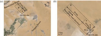
The Qingtu Lake Observation Array (QLOA) is located on the flat dry lake bed of the Qingtu Lake between the Badain Jaran Desert and the Tenger Desert in western China (E:
 $103^{\circ }40^{\prime }03^{\prime \prime }$
, N:
 $39^{\circ }12^{\prime }27^{\prime \prime }$
), as shown in figure 1. This area skirts the pathway of the strong northwest monsoons and sandstorms, which move southward from the Badain Jaran Desert during spring.
Figure 1(a) shows the upwind area of the QLOA site (black dotted lines). It is composed of region A from 0 to 10 km and region B from 10 to 30 km from the site. Figure 1(b) shows an enlargement of regions A and B. In region A, the ground is flat and devoid of vegetation with height variations of less than 1 m. Region B is also devoid of vegetation but has a few barchans (2 m in height). There are less than 5 barchans per kilometre (estimated) in the upwind direction. The minimum distance between two neighbouring dunes is approximately 200 m, which is 100 times the dune height. According to Sauermann, Kroy & Herrmann (Reference Sauermann, Kroy and Herrmann2001), the flow will recover to the free stream condition if the distance from the sand dune is larger than 4 times that of the dune height. Therefore, the barchans in region B should not adversely influence the measurements. Furthermore, the least-square fitting of the mean streamwise wind velocity profile based on the logarithmic law (Clauser Reference Clauser1956) was used to calculated the equivalent sand grain roughness height,
 $k_{s}$
, at the site as
 $2\times 10^{-3}$
m.
Satellite photographs of the QLOA site: (a) observation area and (b) topography in the upwind direction of the site.

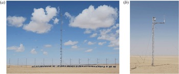
Figure 2(a) shows an overview of the QLOA site. Twenty-one towers are arranged along the prevailing wind direction and the spanwise direction. The main tower is 32 m high and the remaining 20 lower towers are 5 m in height, as shown in figure 2(b). Each tower is comprised of three steel tubes. The tubes were bound by solid steel rods to form triangles with side lengths of
 $l_{1}=0.5$
m and
 $l_{2}=0.2$
m for the main and lower towers. The towers were fixed on cement bases (submerged in the ground) and reinforced by ropes to resist the strong winds. The swinging amplitude is less than
 $0.1^{\circ }$
for a
 $20~\text{m}~\text{s}^{-1}$
wind at 5 m height.
Eight of the 20 low towers were arranged in the prevailing wind direction at equal distances of 30 m (
 $l_{st}=30$
m) from the main tower. The remaining 12 low towers were located on both sides of the main tower (six on each side) in the spanwise direction at equal distances of 5 m (
 $l_{sp}=5$
m). Hence, the three-dimensional velocity distributions could be measured, covering 240, 60 and 32 m in the streamwise, spanwise and vertical directions, respectively. The ratios of the tower separated distance and the side length of the tower cross-section are
 $l_{st}/l_{2}=150$
and
 $l_{sp}/l_{2}=25$
in the streamwise and spanwise directions, which are significantly larger than the required value for neglecting the disturbances of the towers on the flow (Ong & Wallace Reference Ong and Wallace1996). Section 4 will demonstrate and confirm that the current arrangement of towers has little influence on the ASL flow measurements.
Photographs of observation arrays: (a) panoramic view, (b) lower towers.

Thirty-one three-component sonic anemometers (Gill Instruments R3-50) were installed on the towers to synchronously measure the wind velocity and the air temperature (at a sample frequency of 50 Hz). The wind speed measurement range of the anemometer is from 0 to
 $45~\text{m}~\text{s}^{-1}$
, with a minimum resolution of
 $0.01~\text{m}~\text{s}^{-1}$
and a relative error (root-mean-squared) of less than 1 %. The wind direction can be recorded from 0
 $^{\circ }$
to 359
 $^{\circ }$
, with a minimum resolution of 1
 $^{\circ }$
and an absolute error of less than
 $1^{\circ }$
. The temperature can be measured from
 $-40$
to
 $60\,^{\circ }\text{C}$
, with a minimum resolution of
 $1\,^{\circ }\text{C}$
and an error of less than
 $1\,^{\circ }\text{C}$
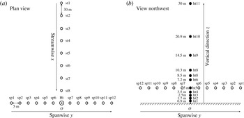
. Figure 3 shows the anemometer arrangement. Eleven anemometers were installed on the main tower at heights from 0.9 to 30 m in a logarithmic manner. On each low tower, only one anemometer was installed at a height of 5 m. In figure 3, a right-handed coordinate system is also presented with a origin
 $O$
at the bottom of the high tower axis, and the
 $x$
,
 $y$
and
 $z$
axes indicate the streamwise, spanwise and vertical directions, respectively. The anemometers were 1.5 m (
 $s_{1}=1.5$
m) and 0.75 m (
 $s_{2}=0.75$
m) from the main and low towers, respectively, with dimensionless distances of
 $s_{1}/l_{1}=3.0$
and
 $s_{2}/l_{2}=3.75$
. According to Dabberdt (Reference Dabberdt1968) and Camp & Kaufman (Reference Camp and Kaufman1970), the influence of the towers on wind velocity measurements by the anemometers can be ignored for
 $s/l>2$
. During the installation, the anemometer coordinates were in accordance with the observation array. For the measurements, 5 anemometers were linked to one data acquisition instrument with the different data acquisition instruments synchronized in time by a global positioning system (GPS).
Schematic of sonic anemometers installation, (a) plan view and (b) northwest view of the sonic anemometer array. The open circles labelled sp
 $i$
(
 $i=1,2,\ldots ,12$
) and st
 $j$
(
 $j=1,2,\ldots ,8$
) represent the spanwise and streamwise anemometers respectively, and the solid circles labelled ht
 $k$
(
 $k=1,2,\ldots ,11$
) represent the anemometers installed on the main tower in the vertical direction.

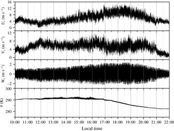
The measurements at the QLOA site were performed for more than 1200 h between 3 April and 25 May 2013. In total, 2.16 Terabyte of wind velocity and temperature data for turbulent ASL flows were recorded. The data from 10:00–22:00 on 7 May 2013 were used to describe the selection and pretreatment process of the measured data (figure 4) in the next section.
The raw data of prevailing wind velocity
 $U_{s}$
, streamwise wind velocity
 $V_{s}$
, spanwise wind velocity
 $W_{s}$
and temperature
 $\unicode[STIX]{x1D703}$
during 10:00–22:00 on 7 May 2013 recorded by the anemometer ht5 on the main tower (5 m from the ground).

3 Data pretreatment
Due to the complexity and uncontrollability of the environmental conditions in field observations, specific selection and pretreatment should be performed on the raw data in order to ensure the reliability for accurate representation of the high Reynolds number turbulent boundary layer. The pretreatment included stratification stability judgment, wind direction adjustment, long-term trend filtering and non-stationary effects exclusion. This section describes these manipulations in detail.
A canonical zero pressure gradient (ZPG) turbulent boundary layer (TBL) is a purely shear-driven flow, while the ASL is usually affected by buoyancy. Therefore, the stratification stability judgment calculated the Monin–Obukhov stability parameter (Stull Reference Stull1988) to select data that satisfied the neutral stratification condition. Also, the actual wind direction did not always accord with the direction of the streamwise towers. Here, if the direction deviation denoted by
 $\unicode[STIX]{x1D6FC}(t)$
(
 $t$
is time) was non-zero, the measured wind velocities were adjusted. Next, long-term synoptic-scale events were filtered out because they were not turbulent fluctuations. In the last step, a quality verification was performed to ensure the wind data were statistically steady and the high-quality requirement of Foken et al. (Reference Foken, Göockede, Mauder, Mahrt, Amiro and Munger2004) was satisfied. According to Hutchins et al. (Reference Hutchins, Chauhan, Marusic, Monty and Klewicki2012), to obtain converged statistics for turbulent flows, the streamwise advection length should be of the order of
 $O(100)$
of the surface layer thickness. When the wind speed was low (e.g.
 $5~\text{m}~\text{s}^{-1}$
), the streamwise advection time scale was usually greater than 50 min but would be smaller for higher wind velocities. Hence, in the current study, the measured data were split into multiple one hour time series for selection, pretreatment and analysis (with statistical convergence as a prerequisite). This data length
 $T_{d}$
also satisfies the statistical steady requirement
 $T_{d}\geqslant 20\unicode[STIX]{x1D6FF}/U_{e}$
of Metzger, McKeon & Holmes (Reference Metzger, McKeon and Holmes2007), where
 $\unicode[STIX]{x1D6FF}$
is the thickness of surface layer,
 $U_{e}$
is horizontal velocity at
 $\unicode[STIX]{x1D6FF}$
. In particular,
 $T_{d}=3600~\text{s}\gg 200{-}300~\text{s}=20\unicode[STIX]{x1D6FF}/U_{e}$
in the present study.
3.1 Stratification stability judgement
The ASL stratification stability is characterized by the ratio of the buoyancy
 $-g\overline{W_{s}\unicode[STIX]{x1D703}}/\bar{\unicode[STIX]{x1D703}}$
and the wind stress
 $u_{\unicode[STIX]{x1D70F}}^{3}/\unicode[STIX]{x1D705}z$
, i.e. the Monin–Obukhov stratification parameter
 $$\begin{eqnarray}\frac{z}{L}=-\frac{\unicode[STIX]{x1D705}zg\overline{W_{s}\unicode[STIX]{x1D703}}}{\bar{\unicode[STIX]{x1D703}}u_{\unicode[STIX]{x1D70F}}^{3}},\end{eqnarray}$$
where
 $z$
is the height,
 $L$
is the Obukhov length,
 $\bar{\unicode[STIX]{x1D703}}$
is the surface average temperature,
 $\unicode[STIX]{x1D705}=0.41$
is the Kármán constant,
 $g$
is the acceleration due to gravity and
 $\overline{W_{s}\unicode[STIX]{x1D703}}$
is the average vertical heat flux which was calculated by averaging the covariance between the vertical wind velocity
 $W_{s}$
and the temperature
 $\unicode[STIX]{x1D703}$
.
 $u_{\unicode[STIX]{x1D70F}}$
is the friction velocity, which was obtained by fitting the mean streamwise velocity profile using the Clauser chart technique (Clauser Reference Clauser1956) with
 $\unicode[STIX]{x1D705}=0.41$
and
 $B=5.0$
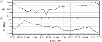
. It is noted that Metzger et al. (Reference Metzger, McKeon and Holmes2007) estimated the friction velocity using the Reynolds stress at a specific height (1.4 m in their study). The present work did not use their method because we found that the Reynolds stress was sensitive to the height in the ASL. Figure 5 shows the stability parameters
 $z/L$
for measured wind velocity (figure 5
a) and the corresponding mean wind direction
 $\unicode[STIX]{x1D6FC}(t)$
(figure 5
b). The wind direction,
 $\unicode[STIX]{x1D6FC}$
, was positive when the wind direction varied in the clockwise direction of the anemometer heading direction. Although the wind directions varied with time, the majority of the data satisfied the requirement
 $|\unicode[STIX]{x1D6FC}|<30^{\circ }$
for the wind direction of Hutchins et al. (Reference Hutchins, Chauhan, Marusic, Monty and Klewicki2012).
Computed (a) Monin–Obukhov stratification parameter
 $z/L$
and (b) mean wind direction
 $\unicode[STIX]{x1D6FC}$
from measured data during 10:00–22:00 on 7 May 2013.

Referring to Högström, Hunt & Smedman (Reference Högström, Hunt and Smedman2002) and Hutchins et al. (Reference Hutchins, Chauhan, Marusic, Monty and Klewicki2012), the stratification stability and steady wind direction criteria used in the present analysis are
 $$\begin{eqnarray}|z/L|<0.06,\quad |\unicode[STIX]{x1D6FC}|<22^{\circ }.\end{eqnarray}$$
It should be noted that the present criteria are more strict than
 $|z/L|<0.1$
adopted by Högström et al. (Reference Högström, Hunt and Smedman2002), Metzger et al. (Reference Metzger, McKeon and Holmes2007) and Hutchins et al. (Reference Hutchins, Chauhan, Marusic, Monty and Klewicki2012).
The stability and wind direction conditions were both satisfied for several time intervals including the interval 17:00–18:00, which was used in subsequent analysis.
3.2 Wind direction adjustment
The wind direction was adjusted using the following formula
 $$\begin{eqnarray}\displaystyle & \displaystyle U_{w}=U_{s}\cos \unicode[STIX]{x1D6FC}+V_{s}\sin \unicode[STIX]{x1D6FC}, & \displaystyle\end{eqnarray}$$
 $$\begin{eqnarray}\displaystyle & \displaystyle V_{w}=V_{s}\cos \unicode[STIX]{x1D6FC}-U_{s}\sin \unicode[STIX]{x1D6FC}, & \displaystyle\end{eqnarray}$$
where
 $U_{s}$
and
 $V_{s}$
are the measured streamwise and spanwise velocities in the anemometer coordinate, and
 $U_{w}$
and
 $V_{w}$
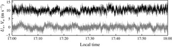
are the actual streamwise and spanwise velocities after adjustment respectively, as shown in figure 6.
The actual streamwise (black line) and spanwise (grey line) velocity components after wind direction adjustment (measured data during 10:00–22:00 on 7 May 2013).

3.3 De-trending manipulation
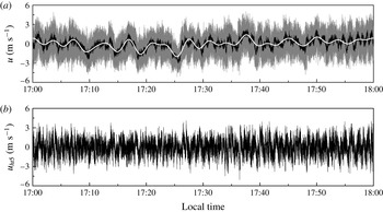
The method introduced by Hutchins et al. (Reference Hutchins, Chauhan, Marusic, Monty and Klewicki2012) for de-trending manipulation was employed after the stratification stability evaluation and wind direction adjustment. First, the measured velocities from 23 anemometers, comprising 11 anemometers on the main tower and 12 anemometers on the spanwise towers, were averaged to obtain the fluctuating streamwise wind velocities. Then, a low-pass filter with a cutoff wavelength of 20
 $\unicode[STIX]{x1D6FF}$
was adopted to obtain the large-scale synoptic wave as in Hutchins et al. (Reference Hutchins, Chauhan, Marusic, Monty and Klewicki2012), where
 $\unicode[STIX]{x1D6FF}$
is the ASL thickness. The synoptic wave was subtracted from the original data to obtain the turbulent fluctuations. Figure 7 shows the large-scale synoptic wave and the de-trended signal.
The method given by Marusic et al. (Reference Marusic, Monty, Hultmark and Smits2013) was used to calculate the ASL thickness
 $\unicode[STIX]{x1D6FF}$
. The streamwise turbulent intensity profiles were calculated by assuming different
 $\unicode[STIX]{x1D6FF}$
based on the formulation of Marusic et al. (Reference Marusic, Monty, Hultmark and Smits2013). Next, a correlation analysis was performed between these profiles and the measured turbulent intensities. The ASL thickness
 $\unicode[STIX]{x1D6FF}$
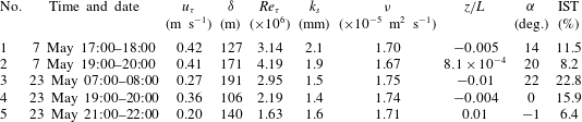
was determined when the correlation coefficient was the largest. Table 1 lists the ASL thicknesses
 $\unicode[STIX]{x1D6FF}$
estimated from different data sets. Further confirmation of the current results are demonstrated by a comparison between the measured turbulent intensity profiles and the predictions by Marusic et al. (Reference Marusic, Monty, Hultmark and Smits2013) (figure 10 in § 4) and by an analysis of the effects of different cutoff wavelengths on the premultiplied spectra (figure 20 in § 5).
Main parameters of the selected ASL measurement data.

De-trending process (measured data during 10:00–22:00 on May 7, 2013): (a) grey line is the streamwise velocity after wind direction adjustment, black line is the streamwise velocity fluctuations and white line is large-scale synoptic wave obtained by low-pass filtering; (b) de-trended signal at ht5.

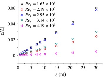
Variations of the Monin–Obukhov stability parameter
 $|z/L|$
with height.

3.4 Steady wind selection
In order to obtain high-quality data for the turbulence statistics analysis, steady wind selection was conducted following Foken et al. (Reference Foken, Göockede, Mauder, Mahrt, Amiro and Munger2004) to calculate the non-stationary index for wind data after direction adjustment and de-trending
 $$\begin{eqnarray}\text{IST}=|(\text{CV}_{m}{-}\text{CV}_{1h})/\text{CV}_{1h}|\times 100\,\%,\end{eqnarray}$$
where
 $\text{CV}_{m}=\sum _{i=1}^{12}\text{CV}_{i}/12$
,
 $\text{CV}_{1}$
,
 $\text{CV}_{2},\ldots ,\text{CV}_{12}$
are the streamwise velocity variances every 5 min in 1 h, and CV1h is the total streamwise velocity variance for the hour. According to Foken et al. (Reference Foken, Göockede, Mauder, Mahrt, Amiro and Munger2004) high-quality data with
 $\text{IST}<30\,\%$
were selected in the present study.
After the steady wind selection, 9 sets of data were verified as stationary and high quality. Five sets then were adopted for further analyses because the Reynolds numbers of some data sets were very similar. Each data set included 1 h velocity time series obtained from 11 heights on the main tower. Figure 8 shows the variations of the Monin–Obukhov stability parameter
 $z/L$
with height for these 5 data sets. It is seen that
 $z/L$
increases with height while the condition
 $|z/L|<0.06$
is satisfied for all heights. Hence, the 5 sets of data are all high-quality data that can be used in high Reynolds number wall turbulence research. Table 1 lists the main parameters of the data. The authors note that the Reynolds numbers reported here are the highest to date for ASL without sand or dust entrainment.
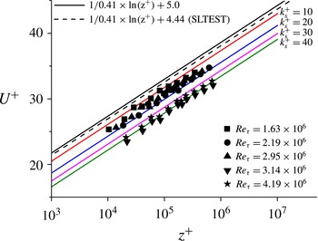
Comparison of mean velocity profiles: black solid symbols are the current data, black solid line is
 $U^{+}=\ln (z^{+})/0.41+5.0$
for smooth-wall wind profile, black dashed line is
 $U^{+}=\ln (z^{+})/0.41+4.44$
according to Marusic et al. (Reference Marusic, Monty, Hultmark and Smits2013) and coloured solid lines are mean velocity profiles with various equivalent roughness
 $k_{s}^{+}$
.

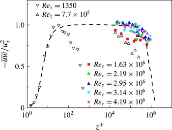
Comparison of Reynolds stress with inner-scaled height: solid symbols are the current data, dashed line is the similarity formulation from Chauhan (Reference Chauhan2007) for
 $Re_{\unicode[STIX]{x1D70F}}=2.33\times 10^{6}$
and open symbols are the field observation and wind tunnel results of Hutchins et al. (Reference Hutchins, Chauhan, Marusic, Monty and Klewicki2012) at
 $Re_{\unicode[STIX]{x1D70F}}=7.7\times 10^{5}$
and Graaff & Eaton (Reference Graaff and Eaton2000) at
 $Re_{\unicode[STIX]{x1D70F}}=1350$
.

4 Validation
In order to confirm that the ASL data from the QLOA site are suitable for the study of high Reynolds number wall-bounded turbulent flows, the variations of the mean streamwise velocity, the Reynolds stress as well as the turbulent intensity with height and Reynolds number were analysed and compared with other experimental and theoretical results of the canonical ZPG TBL flow.
Figure 9 shows the non-dimensional mean streamwise velocity profiles. The measured non-dimensional mean streamwise wind velocities
 $U^{+}=U/u_{\unicode[STIX]{x1D70F}}$
at different heights from all 5 data sets are displayed as solid black symbols, and the solid black line indicates the logarithmic profile over a smooth wall as
 $U^{+}=(1/\unicode[STIX]{x1D705})\ln (z^{+})+B$
, where
 $z^{+}=u_{\unicode[STIX]{x1D70F}}z/\unicode[STIX]{x1D708}$
with
 $\unicode[STIX]{x1D705}=0.41$
and
 $B=5.0$
. As a comparison, the SLTEST result presented by Marusic et al. (Reference Marusic, Monty, Hultmark and Smits2013) is also shown with a dashed black line in figure 9. All the profiles agree with the logarithmic law, despite the down shift
 $\unicode[STIX]{x0394}U^{+}$
due to ground roughness. The roughness effect is illustrated by also plotting the logarithmic profiles with equivalent an sand grain roughness height of
 $k_{s}^{+}=10,20,30$
and
 $40$
to demonstrate that the measured mean streamwise velocities were in good agreement with the rough-wall logarithmic laws. The down-shift values are calculated to be
 $\unicode[STIX]{x0394}U^{+}=2\sim 5$
using the least-squared fitting method mentioned in § 2. The equivalent roughness at the QLOA site was approximately
 $k_{s}^{+}=16\sim 52$
, which indicates that the surface layer was in the transitionally rough regime (
 $k_{s}^{+}<90$
) according to Ligrani & Moffat (Reference Ligrani and Moffat1986).
Kunkel & Marusic (Reference Kunkel and Marusic2006) compared the Reynolds stress spectra obtained with sonic anemometers (20 Hz) and hot-wire anemometers (5000 Hz) to show that the temporal resolution of the sonic anemometer was sufficient for characterizing the Reynolds stress in the ASL (
 $z>0.2~\text{m}$
). Thus, the current data (
 $z>0.9$
m) obtained with the sonic anemometer (sample frequency of 50 Hz) are reliable for Reynolds stress analyses. Figure 10 shows the non-dimensional Reynolds shear-stress profiles for all 5 data sets. The Reynolds shear-stress variations are also in good agreement with the theoretical predictions (Chauhan Reference Chauhan2007; Nagib & Chauhan Reference Nagib and Chauhan2008) for the canonical ZPG TBL flow, represented by the black dash line in figure 10.
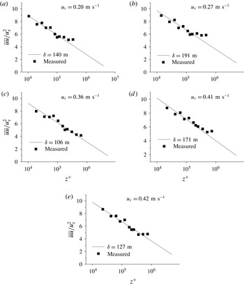
Figure 11 shows the turbulent intensities of the streamwise velocities at different heights (solid squares) together with the formulation
 $\overline{uu}/u_{\unicode[STIX]{x1D70F}}^{2}=2.14-1.33\ln (z/\unicode[STIX]{x1D6FF})$
given by Marusic et al. (Reference Marusic, Monty, Hultmark and Smits2013) (solid line). The boundary layer thicknesses
 $\unicode[STIX]{x1D6FF}$
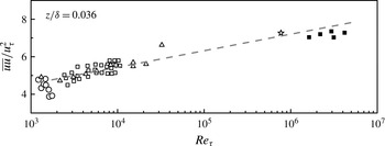
used in the equation were obtained by a best fit of the measured turbulent intensities, they were also taken as the ASL thicknesses in the present study (table 1 in § 3). The measurements agree well with the predictions. Furthermore, the turbulent intensities measured at
 $z/\unicode[STIX]{x1D6FF}\approx 0.036$
(solid squares) were compared to several other measurements, including SLTEST results (Hutchins et al.
Reference Hutchins, Chauhan, Marusic, Monty and Klewicki2012) and wind tunnel experiments (Österlund et al.
Reference Österlund, Johansson, Nagib and Hites2000; Knobloch & Fernholz Reference Knobloch and Fernholz2004; Hutchins et al.
Reference Hutchins, Nickels, Marusic and Chong2009; Kulandaivelu & Marusic Reference Kulandaivelu and Marusic2010) in figure 12. The current results coincide with the extrapolated trend from previous data, indicating an approximate log–linear relationship (the grey dashed line in figure 12) between
 $\overline{uu}/u_{\unicode[STIX]{x1D70F}}^{2}$
and the Reynolds number.
Variation of streamwise turbulent intensity with inner-scaled height: solid squares are current data and black solid lines are the theoretical formulation proposed by Marusic et al. (Reference Marusic, Monty, Hultmark and Smits2013), i.e.
 $\overline{uu}/u_{\unicode[STIX]{x1D70F}}^{2}=2.14-1.33\ln (z/\unicode[STIX]{x1D6FF})$
.

Variation of streamwise turbulent intensity with Reynolds number: solid squares represent current data, open five-pointed star is from Hutchins et al. (Reference Hutchins, Chauhan, Marusic, Monty and Klewicki2012) and other open symbols are from wind-tunnel results of, Österlund et al. (Reference Österlund, Johansson, Nagib and Hites2000), Knobloch & Fernholz (Reference Knobloch and Fernholz2004), Hutchins et al. (Reference Hutchins, Nickels, Marusic and Chong2009) and Kulandaivelu & Marusic (Reference Kulandaivelu and Marusic2010).

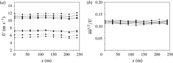
In order to evaluate the influence of upstream towers on the measurement at the main tower, the mean streamwise velocity
 $U$
and the non-dimensional standard deviation of the streamwise velocity fluctuations
 $\sqrt{\overline{uu}}/U$
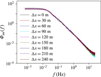
from the streamwise towers are displayed with streamwise distance in figures 13(a) and 13(b). The power spectra of the streamwise velocity fluctuations
 $\unicode[STIX]{x1D6F7}_{uu}$
are shown in figure 14. The turbulence statistics are nearly constant against streamwise distance and the spectra collapse well, which indicates the interference effect from the streamwise lower towers can be ignored.
Sensitivities of (a) mean streamwise velocity
 $U$
at 5 m and (b) non-dimensional standard deviation of streamwise velocity fluctuations
 $\sqrt{\overline{uu}}/U$
with streamwise distance.

Power spectral density of streamwise wind velocity at different streamwise towers.

In summary, the turbulent statistics from the present ASL measurement (mean velocity, Reynolds shear stress and streamwise turbulent intensity) are in good agreement with other measurements and theoretical or empirical predictions for the ZPG TBL flow. Thus, the viability of the current ASL data at the QLOA site to be used in the study of wall-bounded turbulent flows has been confirmed.
5 Results and analysis
This section presents the correlations and spectral analyses of the measured data (5 sets of ASL data after pretreatment) in order to explore the existence, TKE contribution and possible evolution mechanism of VLSMs in high Reynolds number ASL at
 $Re_{\unicode[STIX]{x1D70F}}=(1.63\sim 4.19)\times 10^{6}$
.
5.1 Correlation and spectral analysis of the ASL data
The spatial correlations of the streamwise velocities were analysed (Chauhan Reference Chauhan2007; Hutchins & Marusic Reference Hutchins and Marusic2007a ). The definition of the correlation coefficient is
 $$\begin{eqnarray}R_{ij}(\unicode[STIX]{x0394}x)=\frac{\langle u_{hti}^{\prime }(x)u_{htj}^{\prime }(x+\unicode[STIX]{x0394}x)\rangle }{\unicode[STIX]{x1D70E}_{hti}\unicode[STIX]{x1D70E}_{htj}},\end{eqnarray}$$
in which
 $\text{ht}i$
(
 $i=1,2,\ldots ,11$
) is anemometer height on the main tower,
 $\langle \rangle$
represents the ensemble average,
 $\unicode[STIX]{x1D70E}_{hti}$
is the standard deviation of streamwise velocity fluctuations at
 $\text{ht}i$
,
 $x=\bar{U}_{w}t$
and
 $\unicode[STIX]{x0394}x=\bar{U}_{w}\unicode[STIX]{x0394}t$
are the spatio-temporal transformations using Taylor’s hypothesis,
 $\unicode[STIX]{x0394}t$
is the translational time interval and
 $\bar{U}_{w}$
is the mean advection velocity. In order to demonstrate the existence of the VLSMs,
 $\text{ht}5$
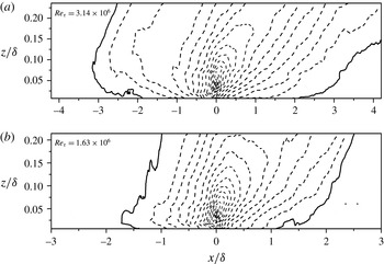
was selected as the reference height. The spatial correlation coefficients between other locations and the reference location were calculated. Figure 15 shows the spatial correlation coefficient contours for the first and last data sets in table 1. According to Hutchins & Marusic (Reference Hutchins and Marusic2007a
), the correlation coefficient contour level indicating the coherent structure edge was set to be 0.05, as the black solid line in figure 15. The streamwise length scale of the detected turbulent structure in figure 15 satisfies
 $|\unicode[STIX]{x0394}x/\unicode[STIX]{x1D6FF}|>3$
, indicating the possible existence of the VLSMs with streamwise length scales 3 times larger than the ASL thickness (Balakumar & Adrian Reference Balakumar and Adrian2007).
Two-point correlation contours of streamwise velocity fluctuations, in which the black solid lines indicate the contour level of
 $R=0.05$
and dashed lines are contour lines of
 $R$
with equal spacing of 0.05 increasingly.

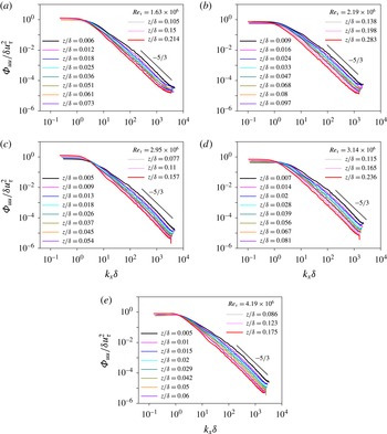
Figure 16 shows the normalized spectra of the streamwise velocity
 $\unicode[STIX]{x1D6F7}_{uu}/\unicode[STIX]{x1D6FF}u_{\unicode[STIX]{x1D70F}}^{2}$
for all 5 data sets at 11 heights. A multi-point averaging procedure was used to smooth the spectra following Balasubramaniam (Reference Balasubramaniam2005) and Taylor’s hypothesis (Taylor Reference Taylor1938) for the spatio-temporal transformations. Figure 16(a–e) shows that, in the region for
 $k_{x}\unicode[STIX]{x1D6FF}<2$
(wavelength larger than
 $3\unicode[STIX]{x1D6FF}$
), all the spectral curves have individual inflection points at which the slope of spectral curves change obviously. Here
 $k_{x}=2\unicode[STIX]{x03C0}/\unicode[STIX]{x1D706}_{x}$
is the wavenumber and
 $\unicode[STIX]{x1D706}_{x}$
is the streamwise wavelength. According to
 $\unicode[STIX]{x1D706}_{x}/\unicode[STIX]{x1D6FF}=2\unicode[STIX]{x03C0}/(k_{x}\unicode[STIX]{x1D6FF})$
, if
 $k_{x}\unicode[STIX]{x1D6FF}<2$
, we have
 $\unicode[STIX]{x1D706}_{x}/\unicode[STIX]{x1D706}>\unicode[STIX]{x03C0}>3$
. The inflection point corresponds to the spectral peak in low-wavenumber region of the premultiplied spectrum (as shown in figure 21) which is associated with the VLSMs (Kim & Adrian Reference Kim and Adrian1999; Vallikivi et al.
Reference Vallikivi, Ganapathisubramani and Smits2015a
). Therefore, it is also demonstrated that the VLSMs exist in all 5 sets of the current ASL data at
 $Re_{\unicode[STIX]{x1D70F}}\sim O(10^{6})$
.
Power spectra of streamwise velocity fluctuations
 $\unicode[STIX]{x1D6F7}_{uu}/\unicode[STIX]{x1D6FF}u_{\unicode[STIX]{x1D70F}}^{2}$
versus streamwise wavenumber
 $k_{x}\unicode[STIX]{x1D6FF}$
. The
 $-5/3$
slope is also displayed.

The correlations and spectral analyses of the current ASL measurement confirm the existence of VLSMs which supports the conclusions of Hutchins & Marusic (Reference Hutchins and Marusic2007a ) and Hutchins et al. (Reference Hutchins, Chauhan, Marusic, Monty and Klewicki2012). Furthermore, the contour lines of correlation coefficient are tilted along the streamwise direction, indicating that the inclination of the turbulent structures observed by Marusic & Heuer (Reference Marusic and Heuer2007) also present in the current ASL measurements at higher Reynolds numbers.
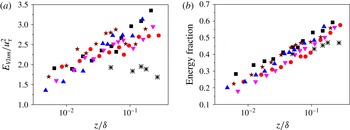
The turbulent energy of VLSMs,
 $E_{Vlsm}$
, and their fraction of the total streamwise TKE, are plotted against height using low-pass filtering with a cutoff length of
 $3\unicode[STIX]{x1D6FF}$
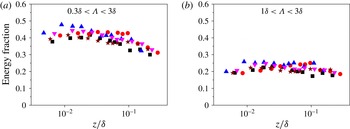
, as shown in figure 17. For comparison, band-pass filtering with cutoff lengths of
 $0.3\unicode[STIX]{x1D6FF}{-}3\unicode[STIX]{x1D6FF}$
(Guala et al.
Reference Guala, Hommema and Adrian2006) and
 $\unicode[STIX]{x1D6FF}{-}3\unicode[STIX]{x1D6FF}$
(Lee, Ahn & Sung Reference Lee, Ahn and Sung2015) were also used to demonstrate the energy fractions of the LSMs with length scales less than
 $3\unicode[STIX]{x1D6FF}$
as shown in figure 18.
Variations of total energy and energy fraction of VLSMs with height (▪, ▴, ▾, ● and
 $\star$
represent present results at
 $Re_{\unicode[STIX]{x1D70F}}=1.63\times 10^{6}$
,
 $2.19\times 10^{6}$
,
 $2.95\times 10^{6}$
,
 $3.14\times 10^{6}$
,
 $4.19\times 10^{6}$
respectively;
 $\ast$
are computed from premultiplied spectral results of Balakumar & Adrian (Reference Balakumar and Adrian2007) at
 $Re_{\unicode[STIX]{x1D70F}}=2395$
).

Variations of energy fraction of turbulent structure with height (▪, ▴, ▾, ● and
 $\star$
represent present results at
 $Re_{\unicode[STIX]{x1D70F}}=1.63\times 10^{6}$
,
 $2.19\times 10^{6}$
,
 $2.95\times 10^{6}$
,
 $3.14\times 10^{6}$
,
 $4.19\times 10^{6}$
respectively).

Figure 17(a) shows that the normalized turbulent energy of the VLSMs increases with the wall-normal distance in an approximately log–linear manner. This is qualitatively different from the wind tunnel results at
 $Re_{\unicode[STIX]{x1D70F}}=2395$
of Balakumar & Adrian (Reference Balakumar and Adrian2007), where the turbulent energy of the VLSMs did not significantly vary with height (star symbols in figure 17(a)). The energy fraction of the VLSMs from the present measurements and the wind tunnel measurements of Balakumar & Adrian (Reference Balakumar and Adrian2007) both increase with height. However, the slope of the latter is smaller. The disparity in figure 17(a) is mainly due to different variations of the energy contribution from the VLSMs with height between the current ASL data and other studies (further analysis and discussion will be given below). Although Taylor’s hypothesis (Taylor Reference Taylor1938) was utilized for the spatio-temporal transformation, according to del Alamo & Jiménez (Reference del Alamo and Jiménez2009), Tayler’s hypothesis transformation only affects the spectral energy distribution in low-wavenumber region (not the integrated energy of the VLSMs). Thus, Taylor’s hypothesis has little influence on the obtained total energy of the VLSMs.
The energy fraction from the LSMs slightly decreases or varies little with height (figure 18). The VLSMs contribute approximately 20 %–30 % and the LSMs contribute 40 % of the total streamwise TKE in the near-wall region of
 $z/\unicode[STIX]{x1D6FF}<0.01$
. While the energy fraction of the VLSMs rapidly increases with height, LSMs decrease. The TKE contribution from the VLSMs can reach as high as 60 % at
 $z=0.2\unicode[STIX]{x1D6FF}$
, which is higher than 40 %–50 % as reported by Guala et al. (Reference Guala, Hommema and Adrian2006), Balakumar & Adrian (Reference Balakumar and Adrian2007) and Lee & Sung (Reference Lee and Sung2011).
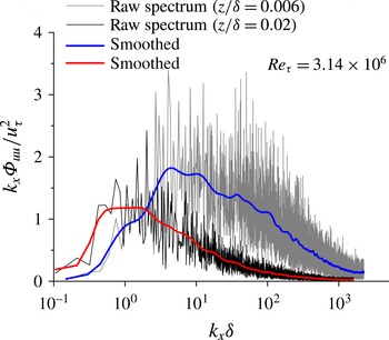
Premultiplied spectra before and after smoothing for the data set 5 in table 1.

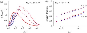
(a) The premultiplied spectra and (b) energy fractions by different de-trending cutoff lengths of
 $20\unicode[STIX]{x1D6FF}$
(black),
 $16\unicode[STIX]{x1D6FF}$
(blue) and
 $24\unicode[STIX]{x1D6FF}$
(red). The solid line, dashed line and dotted line in (a) represent spectra at
 $z/\unicode[STIX]{x1D6FF}=0.007$
, 0.028 and 0.236 respectively.

5.2 Premultiplied spectral analysis
Methods similar to those of Kim & Adrian (Reference Kim and Adrian1999), Hutchins & Marusic (Reference Hutchins and Marusic2007a
), Mathis et al. (Reference Mathis, Hutchins and Marusic2009) and Vallikivi et al. (Reference Vallikivi, Ganapathisubramani and Smits2015a
) were used for premultiplied spectral analyses of the present ASL data. It was found that the premultiplied spectra of raw data fluctuated significantly (figure 19). According to Metzger (Reference Metzger2006) and Kunkel & Marusic (Reference Kunkel and Marusic2006), smoothing operations for the raw premultiplied spectra were performed. The main steps were as follows. Firstly, the non-dimensional wavenumber
 $k_{x}\unicode[STIX]{x1D6FF}$
was taken as the independent variable. The data points used in a smoothing window increase with
 $k_{x}\unicode[STIX]{x1D6FF}$
as
 $N_{s}=\text{int}(2\log (k_{x}\unicode[STIX]{x1D6FF}))+5$
where int denotes the integer rounding operation. Thus, there were less data points in a low-wavenumber smoothing window. For example, there were approximately 3 points for
 $k_{x}\unicode[STIX]{x1D6FF}\sim 0.1$
while 11 points for
 $k_{x}\unicode[STIX]{x1D6FF}\sim 1000$
. Secondly, a linear least-squared fitting method was employed in each window to determine the spectral densities. This smoothing procedure was repeated 10 times to obtain the final smoothed premultiplied spectra (the blue and red lines in figure 19). The trends in the smoothed premultiplied spectra are in good agreement with the presmoothed spectra.
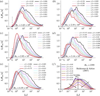
Premultiplied spectra for streamwise velocity fluctuation
 $k_{x}\unicode[STIX]{x1D6F7}_{uu}/u_{\unicode[STIX]{x1D70F}}^{2}$
, versus streamwise wavenumber
 $k_{x}\unicode[STIX]{x1D6FF}$
: (a–e) are current data at various Reynolds numbers, and (f) is laboratory TBL data at
 $Re_{\unicode[STIX]{x1D70F}}=2395$
of Balakumar & Adrian (Reference Balakumar and Adrian2007).

The effects of the de-trending (§ 3) on the premultiplied spectra were evaluated by comparing the smoothed spectra with 3 different de-trending cutoff lengths of
 $16\unicode[STIX]{x1D6FF}$
,
 $20\unicode[STIX]{x1D6FF}$
and
 $24\unicode[STIX]{x1D6FF}$
in figure 20(a). Although there are some differences in the low-wavenumber range, the shape and variation of spectra with height are not significantly affected by the different cutoff values. In addition, figure 20(b) shows the energy fractions for length scales of
 $\unicode[STIX]{x1D6EC}>\unicode[STIX]{x1D6FF}$
and
 $\unicode[STIX]{x1D6EC}>3\unicode[STIX]{x1D6FF}$
with the de-trending cutoff length scales of
 $16\unicode[STIX]{x1D6FF}$
,
 $20\unicode[STIX]{x1D6FF}$
and
 $24\unicode[STIX]{x1D6FF}$
. The results are in good agreement both qualitatively and quantitatively. Therefore, using
 $20\unicode[STIX]{x1D6FF}$
as the de-trending cutoff length in the present study should have little influence on the premultiplied spectral analysis.
Figure 21(a–e) shows the smoothed premultiplied spectra for all 5 ASL data sets, as well as the turbulent boundary layer results from the wind tunnel experiments of Balakumar & Adrian (Reference Balakumar and Adrian2007) at
 $Re_{\unicode[STIX]{x1D70F}}=2395$
, as shown in figure 21(f). A distinct peak in the low-wavenumber region that corresponds to the VLSMs (Kim & Adrian Reference Kim and Adrian1999; Guala et al.
Reference Guala, Hommema and Adrian2006; Rosenberg et al.
Reference Rosenberg, Hultmark, Vallikivi, Bailey and Smits2013; Vallikivi et al.
Reference Vallikivi, Ganapathisubramani and Smits2015a
) is observed in the spectra of all the heights and Reynolds numbers. Although another peak corresponding to the LSMs is also observed in other studies (Balakumar & Adrian Reference Balakumar and Adrian2007; Hutchins & Marusic Reference Hutchins and Marusic2007a
; Mathis et al.
Reference Mathis, Hutchins and Marusic2009), this peak is difficult to distinguish in the current ASL data, which is similar to the recent results of Vallikivi et al. (Reference Vallikivi, Ganapathisubramani and Smits2015a
) on a turbulent boundary layer at
 $Re_{\unicode[STIX]{x1D70F}}=72\,500$
. Hence, detection of the peak corresponding to the LSMs is a problem that requires further investigation, especially for high Reynolds number turbulent flows. Despite this, the distinct peak corresponding to VLSMs indicates that VLSMs may be the more dominant structures than the in high Reynolds number ASL flows.
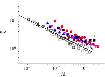
Variation of VLSMs peak wavenumber with height (▪, ▴, ▾, ● and
 $\star$
represent present results at
 $Re_{\unicode[STIX]{x1D70F}}=1.63\times 10^{6}$
,
 $2.19\times 10^{6}$
,
 $2.95\times 10^{6}$
,
 $3.14\times 10^{6}$
,
 $4.19\times 10^{6}$
respectively, open symbols represent TBL results of Vallikivi et al. (Reference Vallikivi, Ganapathisubramani and Smits2015a
) at
 $Re_{\unicode[STIX]{x1D70F}}=72\,500$
, and solid line is their linear fitting).

Figure 21(a–e) also shows that the peak corresponding to the VLSMs moves to a smaller
 $k_{x}\unicode[STIX]{x1D6FF}$
as height increases. The wavenumber of the peak is plotted against non-dimensional height
 $z/\unicode[STIX]{x1D6FF}$
in figure 22, as well as the recent turbulent boundary layer results of Vallikivi et al. (Reference Vallikivi, Ganapathisubramani and Smits2015a
). The peak was determined by local Gaussian fitting method for the premultiplied spectra in semi-log coordinates following Rosenberg et al. (Reference Rosenberg, Hultmark, Vallikivi, Bailey and Smits2013). Here, the wavenumber of the peak decreases with height in an approximately log–linear manner, implying the streamwise length scale of the VLSMs increases with height in the present study, which is consistent with Vallikivi et al. (Reference Vallikivi, Ganapathisubramani and Smits2015a
).
Figure 21(a–e) further shows that the product of the power spectra and the wavenumber
 $k_{x}\unicode[STIX]{x1D6F7}_{uu}$
decreases with height on the right side of the peak in the premultiplied spectra. On the left side of the peak (the low-wavenumber region of the premultiplied spectra),
 $k_{x}\unicode[STIX]{x1D6F7}_{uu}$
increases with height, which is opposite to both the turbulent boundary layer measurement in a tunnel at
 $Re_{\unicode[STIX]{x1D70F}}=2395$
(Balakumar & Adrian Reference Balakumar and Adrian2007) (figure 21
f) and also experiments at higher Reynolds numbers, such as Guala et al. (Reference Guala, Hommema and Adrian2006) for pipe flow at
 $Re_{\unicode[STIX]{x1D70F}}=19\,000$
and Vallikivi et al. (Reference Vallikivi, Ganapathisubramani and Smits2015a
) for the turbulent boundary layer flow at
 $Re_{\unicode[STIX]{x1D70F}}=72\,500$
(where
 $k_{x}\unicode[STIX]{x1D6F7}_{uu}$
all decreased with height throughout the entire spectra). It is possible that the current result is a consequence of using Taylors hypothesis with the mean streamwise velocity as the advection velocity for the spatio-temporal transformation. For example, del Alamo & Jiménez (Reference del Alamo and Jiménez2009) found that the mean streamwise velocities may underestimate the advection velocity for large wavelengths in the buffer and inner logarithmic layers, which could shift the spectral curve at lower heights to the high-wavenumber region (giving the current results). However, the authors believe this is highly unlikely. Figure 17 shows that the absolute energy contribution from the VLSMs increases with height, this means that the energy at higher heights should be larger than lower heights on the left side of the peak. Therefore, the increase of the spectral turbulent energy
 $k_{x}\unicode[STIX]{x1D6F7}_{uu}$
with height in the low-wavenumber region should not be affected by Taylor’s hypothesis.
The decrease of the spectral turbulent energy
 $k_{x}\unicode[STIX]{x1D6F7}_{uu}$
with height in the high-wavenumber region was successfully explained by the ‘bottom-up’ mechanism (Kim & Adrian Reference Kim and Adrian1999), the LSMs or VLSMs grow upwards from the organization of near-wall cycle and turbulent kinetic energy produced in near-wall region gradually dissipates, so that the corresponding VLSMs weaken in the wall-normal direction. However, the increase of the spectral turbulent energy
 $k_{x}\unicode[STIX]{x1D6F7}_{uu}$
with height in the low-wavenumber region is not readily explained by the ‘bottom-up’ mechanism. As stated by Hutchins & Marusic (Reference Hutchins and Marusic2007a
), Morrison (Reference Morrison2007) and Mathis et al. (Reference Mathis, Hutchins and Marusic2009), the interpretation of the evolution of VLSMs at high Reynolds numbers may be incomplete. Thus, there may exist another mechanism to drive the energy transfer of the VLSMs moving downwards. One possible candidate is the ‘top-down’ mechanism proposed by Hunt & Morrison (Reference Hunt and Morrison2000), where VLSMs originate in the outer region of the turbulent boundary layer, carry energy to move downwards, then break into smaller structures due to strong shear in the near-wall region. However, the ‘top-down’ mechanism is still regarded as pure conjecture (Hutchins & Marusic Reference Hutchins and Marusic2007a
). This new result of the energy increasing with height in the low-wavenumber region in the current ASL data is a specific phenomenon at high Reynolds numbers (
 $Re_{\unicode[STIX]{x1D70F}}>10^{6}$
) in ASL, and further investigations are required to understand the physical mechanism.
6 Conclusions
This paper introduced a field observation facility named the Qingtu Lake Observation Array (QLOA), consisting of a main tower of 32 m high and 20 low towers of 5 m high (8 of the low towers were in the streamwise direction and the other 12 in the spanwise direction). Sonic anemometers on the towers synchronously measured three components of the wind velocity as well as the temperature. A total of 1200 h of wind velocity data in clean wind at
 $Re_{\unicode[STIX]{x1D70F}}\sim O(10^{6})$
were acquired. Five sets of high-quality data at
 $Re_{\unicode[STIX]{x1D70F}}=(1.63\sim 4.19)\times 10^{6}$
of 1 h duration for each were finally selected. The selected data were validated for variations of mean streamwise velocity, Reynolds stress and turbulent intensity with height, to be suitable for the research of canonical wall-bounded turbulent flows. The VLSMs were confirmed to exist in the ASL at Reynolds number
 $Re_{\unicode[STIX]{x1D70F}}\sim O(10^{6})$
. Even at such high Reynolds numbers, some results were similar to those at lower Reynolds numbers (
 $Re_{\unicode[STIX]{x1D70F}}<10^{6}$
), e.g. the non-dimensional wavenumber of the outer peak in premultiplied spectra decreases with height in an log–linear manner. Some differences were also observed. For example, the turbulent energy in the low-wavenumber region of the premultiplied spectra increases with height in the present study, while this was seen to decrease with height in previous experiments at
 $Re_{\unicode[STIX]{x1D70F}}<10^{5}$
. As a result, the TKE contribution by the VLSMs increases log–linearly with height, and can reach as high as 60 % of the total TKE. While it should be noted that the sampling rate is 50 Hz in the present study, which means that the TKE of some small-scale motions was not accounted for, so that the 60 % TKE contribution by the VLSMs may be an overestimate. This issue needs further clarification. The differences for the spectra as well as the TKE distributions might imply that, in high Reynolds number ASL flows at
 $Re_{\unicode[STIX]{x1D70F}}\sim O(10^{6})$
, the evolution of the VLSMs may not be attributed to the ‘bottom-up’ mechanism completely, and other mechanisms (e.g. the ‘top-down’ mechanism of Hunt & Morrison (Reference Hunt and Morrison2000)) may exist or coexist with the ‘bottom-up’ mechanism. This warrants further investigation in future. In addition, it should be noted that the surface layer thickness was not directly measured in the present study, which could induce errors for the estimation of Reynolds number. However, we analysed the effect of surface layer thickness by using
 $\unicode[STIX]{x1D6FF}=60$
m, the same as that at SLTEST (Marusic et al.
Reference Marusic, Monty, Hultmark and Smits2013), and found the main conclusions of the present work still hold.
Acknowledgements
This work was supported financially by grants from the National Natural Science Foundation of China (nos 11490553, 11232006 and 11121202). The authors are grateful for the insightful discussions with Dr P. Wang, Mr H.-Y. Liu and Mr G.-W. Han, as well as the helpful comments from three anonymous referees which lead to a significant improvement of the paper.