2. The fluid–body coupling

In the boundary-layer scenario, fluid is flowing along an effectively flat surface, or wall, and far from the wall the free stream is moving with a given constant velocity parallel to that wall. This is locally on an airfoil surface, for example, or on a more general surface. The working below for the flow around a comparatively thin short body moving freely near the wall is expressed in terms of non-dimensional flow velocities $(u,v)$, corresponding Cartesian coordinates $(x,y)$, time $t$ and pressure $p$, such that the dimensional versions are $\tilde {U}(u,v)$, $\tilde {L}(x,y)$, $\tilde {L} t/\tilde {U}$ and (to within an additive constant) $\tilde {\rho } {\tilde {U}}^{2} p$ respectively. Here $\tilde {U}$ is the representative fluid velocity, taken to be the free-stream value, while $\tilde {L}$ is the airfoil chord, $\tilde {\rho }$ is the uniform density of the incompressible fluid and the temporal factor $\tilde {L}/\tilde {U}$ taken is the typical transport time. The velocity vector $(u,v)$, pressure $p$ and coordinates $x,y$ are generally of order unity except near the wall which locally is positioned along the axis $y = 0.$ In particular $(u,v)$ is given by $(1,0)$ in the far field and the leading edge of the airfoil is taken as the origin. The Reynolds number is given by $Re = \tilde {U} \tilde {L}/\tilde {\nu }$ where $\tilde {\nu }$ is the uniform kinematic viscosity of the fluid. The representative length of the body is $\ell$ which is $\tilde {\ell }/\tilde {L}$ and the primary concern is with the properties induced for a short body for which $\ell$ is small, when the Reynolds number is comparatively large. The body is generally translating upstream or downstream but only at a slow rate and so over the time scales of current interest the body is present at an effectively constant order-unity distance $x_0$ say downstream from the airfoil leading edge.

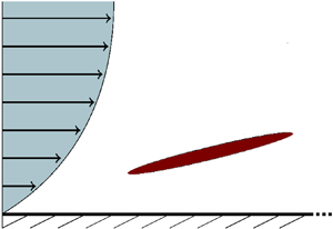
For large values of the Reynolds number $Re$, the thin boundary layer set up along the undisturbed surface ahead of the near-wall body and also downstream of it is a classical one having $x$ scale of order unity. The $y$ scale is of order $Re^{-1/2}$, with $u,p$ variations of $O(1)$ and $v$ being of $O(Re^{-1/2})$. The time scale there is of order unity. This boundary layer and its local free stream form the oncoming and surrounding flow field for the body/fluid interactive motion as in figure 1. The main range of interest is for scaled lengths such that

(2.1)\begin{equation} Re^{-3/4} \ll \ell \ll Re^{-3/8}.\end{equation}

The range of validity in (2.1) (Smith Reference Smith1976; Smith & Daniels Reference Smith and Daniels1981) is actually quite a large one in terms of the scales covered. Notably, the lower limit in (2.1) leads to a local problem governed by the full Navier–Stokes equations with very small $x - x_0$ and $y$ values of order $Re^{-3/4}$ corresponding to a tiny particle. At the other extreme triple-deck theory applies. In between the two extremes, orders of magnitude show that a thin wall sublayer of thickness $O(l^{1/3} Re^{-1/2})$ is present (see figures 1a and 1b) with typical pressure variation being of order $l^{2/3}$: the displacement of the flow just outside the boundary layer due to the dominant $O(l^{2/3})$ pressure variation inside the boundary layer is then of order $l^{5/3}$ and this is small compared with the sublayer thickness which is $O(l^{1/3} Re^{-1/2})$ provided $l \ll Re^{-3/8}$ as in (2.1). The flow structure for the range (2.1) is thus concentrated primarily in the thin sublayer surrounding the moving body as in figures 1(a) and 1(b). In the sublayer at leading order

(2.2)\begin{equation} \left.\begin{gathered} (u,v,p) = \left(\ell^{1/3}U, \ell^{-1/3} Re^{-1/2} V, \ell^{2/3} P \right), \\ \text{with}\quad x-x_0 = \ell X, \ y = \ell^{1/3} Re^{-1/2} Y, \ t = \alpha \ell^{2/3} T, \end{gathered}\right\}\end{equation}

where the large constant $\alpha$ is to be determined and the capital-lettered quantities are of order unity. The body at an unknown position near the wall occupies the interval $0 < X < 1$ in a frame translating slowly streamwise with the body, with the body thickness being comparable with the sublayer height.

Figure 1.

(a,b) Sketch of the freely moving body within a viscous–inviscid wall layer and the resulting flow structure. The height $W$ is the scaled normal distance from the straight wall to the leading edge of the body.

The Navier–Stokes equations then reduce to the quasi-steady condensed-flow interaction (Smith Reference Smith1976; Smith & Daniels Reference Smith and Daniels1981) in which

(2.3a)\begin{gather} U=\varPsi_Y,\quad V = -{\varPsi}_X, \end{gather}

(2.3b)\begin{gather}UU_X + VU_Y=-P_X(X,T)+U_{YY} , \end{gather}

within the gap $I$ underneath the body and within the layer $II$ above the body. Here $\varPsi$ is the streamfunction. The unknown scaled pressure $P(X,T)$ is independent of $Y$ because of the normal-momentum equation in each layer, such that

(2.3c)\begin{equation} P=P^{+}(X,T), \ P = P^{-}(X,T)\ \mbox{above and below the body respectively}. \end{equation}

The relevant boundary conditions are

(2.4a)\begin{gather} U = U_w, \quad V = 0\quad \mbox{at}\ Y=0 , \end{gather}

(2.4b)\begin{gather}U = V = 0\quad \mbox{at}\ Y = F^{-}(X,T) , \end{gather}

(2.4c)\begin{gather}(U,P) = \left( \lambda Y + U_w + a, \frac{U_w^{2}}{2} - \frac{(U_w + a)^{2}}{2} \right)\quad \mbox{at}\ X = 0^{+} , \end{gather}

in the gap $I$. Herein the superscripts $+/-$ refer to the properties on top of and underneath the body in turn. The requirements (2.4a,b) stem from the no-slip conditions at the wall and on the moving under-surface $F^{-}$ of the body. The effective streamwise velocity $U_w$ of the wall is associated with the translation velocity $u_c$ of the body relative to the wall: clearly if the body is translating upstream relative to the wall then $U_w$ is positive. The conditions in (2.4c) are due to an unknown pressure jump arising across an Euler region (Smith et al. Reference Smith, Ovenden, Franke and Doorly2003) which surrounds the leading edge $X=0$, with a corresponding jump $a = a(T)$ being induced in the streamwise velocity $U$ to satisfy the quasi-steady Bernoulli balance. We should emphasise that the jump $a(T)$ is to be determined as part of the solution. The positive $O(1)$ factor $\lambda$ in (2.4c) is the given scaled incident WSS, namely $Re^{-1/2} (\partial u/ \partial y)$ at $y=0$, in the surrounding boundary layer locally, as in figures 1(a) and 1(b) but allowing here for the moving frame. The Euler region is similar to that in Smith et al. (Reference Smith, Ovenden, Franke and Doorly2003) and Jones & Smith (Reference Jones and Smith2003), its streamwise extent being of order $\ell ^{1/3} Re^{-1/2}$. In summary, the physical need for the unknown pressure jump in (2.4c) at the leading edge stems from the upstream influence due to conditions at the trailing edge and mass conservation beneath the body. In the flow $II$ on top of the body, by contrast, we have

(2.5a)\begin{gather} U = V = 0\quad \mbox{at}\ Y = F^{+}(X,T) , \end{gather}

(2.5b)\begin{gather}U \sim \lambda Y + U_w\quad \mbox{as}\ Y \rightarrow \infty , \end{gather}

(2.5c)\begin{gather}(U,P) = \left(\lambda Y + U_w, \lambda a W \right)\quad \mbox{at}\ X = 0^{+} . \end{gather}

The condition (2.5a) is for no slip on the top moving surface of the body. The function $F^{+}$ denotes the unknown scaled position of the body's top surface which is addressed further just below. The requirement (2.5b) of effectively zero displacement in $Y$ corresponds to the feedback effect from the flow outside the sublayer being relatively small and is in keeping with the range specified in (2.1). Condition (2.5c) again comes from the Euler jump in pressure and in velocity, subject to mass conservation at the body surface and to the zero displacement associated with (2.5b); conservation of vorticity is assured because of the local $\lambda Y$ variation throughout. The term $W$ is the scaled width of the gap at, or the height of, the leading edge of the body and is in general an unknown function $W=W(T)$ of the scaled time.

We should comment additionally on certain features. The body, to repeat, is translating with a small constant velocity $u_c$ which is assumed to be comparable with the fluid flow velocity in (2.2) and thus gives rise to the scaled wall velocity $U_w$ in the moving frame, where $u_c = -\ell ^{1/3} U_w$. Hence $U_w$ can be positive or negative. The incident flow at $X=0^{-}$ is one of constant shear with a velocity profile $U = \lambda Y + U_w$ for all $Y\geq 0$ and is at zero pressure. The different pressures $P^{+}$ and $P^{-}$ induced above and below the body act to move the body as described below. The moving surface shapes $F^{+}$ and $F^{-}$ are given specifically by

(2.6a)\begin{equation} F^{\pm} (X,T) = g^{\pm}(X) + h(T) + ( X-\tfrac{1}{2}) \theta(T) .\end{equation}

Here $g^{\pm } (X)$ are the prescribed solid body shapes, atop and underneath, independent of $T$, whereas $h(T)$, $\theta (T)$ account for the evolving normal height and azimuthal rotation of the midpoint of the body. We deal with non-blunt bodies in the sense that $g^{\pm }$ are equal at $X=0$, and can be set to zero there without loss of generality; hence $F^{\pm }$ are equal there, leading to the relation

(2.6b)\begin{equation} W(T) = h(T) - \tfrac{1}{2} \theta(T) ,\end{equation}

between $W,h$ and $\theta$. Along with this the values $g^{\pm }$ are taken to be equal at the trailing edge $X = 1$. Further, given that $\varPsi$ is zero at the wall, we note also the value

(2.6c)\begin{equation} \varPsi = \frac{\lambda W^{2}}{2} + (U_w + a) W\end{equation}

holds for all $0 < X < 1$ at the under and top surfaces of the body from integration of (2.4c) across the gap. This value can also be used with (2.4c), (2.5c) to set the value of the streamfunction for all $Y$ values at $X=0^{+}$. Finally the condition

(2.6d)\begin{equation} P^{+} = P^{-}\quad \mbox{at}\ X = 1 \end{equation}

applies, since there can be no pressure difference across the wake behind the body and a Kutta condition of smooth departure of the flow from the trailing edge is imposed.

The body moves as it responds to the surrounding fluid flow via the differential pressure forcing at the top and under surfaces of the body. The body motion is controlled by

(2.7a)\begin{gather} M h_{TT} = \int_0^{1} \left( P^{-}(X,T) - P^{+}(X,T) \right) \textrm{d}X (= C_L), \end{gather}

(2.7b)\begin{gather}J \theta_{TT} = \int_0^{1} (X - \tfrac{1}{2}) \left( P^{-}(X,T) - P^{+}(X,T) \right) \textrm{d}X (= C_M), \end{gather}

owing to the rates of change in the normal and angular momenta of the body. The mass $\tilde {M}$ of the body is equal to $\alpha ^{2} \tilde {\rho } {\tilde {L}}^{2} \ell ^{8/3} Re^{1/2} M$ with $M$ being of order unity, and likewise the scaled moment of inertia $J$ is $O(1)$. The centre of mass is taken as fixed at $X = 1/2$, which is a main case associated with a body of uniform density and any shape length-wise symmetrical about the midpoint for example. The overall time scale is based on the body motion. As an estimate $\tilde {M}$ is approximately $\tilde {\rho }_B \tilde {V}$ in two dimensions where $\tilde {\rho }_B$ is the density of the body and the effective cross-sectional area $\tilde {V}$ is the product of the $x$ and $y$ scales in (2.2) multiplied by ${\tilde {L}}^{2}$ through non-dimensionalisation. Hence $\alpha ^{2}$ is comparable with $Re^{-1} \ell ^{-4/3} \tilde {\rho }_B /\tilde {\rho }$. This means that the flow behaviour remains quasi-steady provided the density ratio $\tilde {\rho }_B/\tilde {\rho } \gg Re \ell ^{4/3}$. Since the length $\ell$ is $O(Re^{-m})$ where $3/8 < m < 3/4$ from (2.1), the density ratio must exceed $Re^{n}$ where $0 < n < 1/2$ (here $n$ is $1 - 4m/3$) and so the theory is valid over a wide range of density ratios. Further in (2.7a,b) the $P^{+}$ and $P^{-}$ responses are those produced by the fluid flow as described in (2.3a)–(2.6d), thus provoking fluid–body interaction. In the streamwise direction the body momentum and the relatively small fluid-flow forces are consistent with the body velocity $u_c$ and hence the relative wall velocity $U_w$ being constant as assumed earlier.

The central problem of the current fluid–body interaction is to solve (2.3a)–(2.7b). This is a nonlinear near-wall coupling which involves effects from viscous and inviscid dynamics. Our concern is with $W$ being of order unity as opposed to the range of large $W$ values considered by Palmer & Smith (Reference Palmer and Smith2019). The argument has been presented for a boundary-layer setting. A similar setting holds for channel flow and yields the same problem, with scale ranges being different from (2.1) and showing that to leading order there is no influence from the opposite wall of the channel. The interaction can also be expressed more broadly in terms of the local incident shear value alone. The present paper addresses numerical and analytical properties for a flat-plate body in the next two sections.

3. Numerical method and solutions

The numerical work used finite differencing based on a semi-implicit scheme for the two boundary-layer calculations required at each time step. At each $X$ station the scheme iterates for the $P^{\pm }$ values in order to satisfy all the boundary conditions in the normal direction. A two-stepping procedure as in Smith & Timoshin (Reference Smith and Timoshin1996) is adopted to achieve second-order accuracy. In the normal direction we transformed $\eta = Y / F^{-}$ in the fluid-filled gap region $I$ and $\bar {Y} = Y - F^{+}$ in the region $II$ on top of the body. In each region analysis for small positive $X$ indicates that Blasius-like sublayers arise on each solid surface, thus occurring at the wall and at the underbody and overbody surfaces. The scheme coped satisfactorily with these irregularities by means of a transformation $X \rightarrow X^{1/2}$ to render all the sublayer normal coordinates linear in the transformed $X$ coordinate and a sufficiently fine normal discrete step $\delta \eta$ or $\delta \bar {Y}$ to capture the Blasius-like local forms. Concerning streamwise marching the scheme in essence guessed the value of the slip jump $a$, marched forward successively in $X$ and iterated on the $a$ value in order to meet the Kutta requirement. The scheme sets the small spatial steps $\delta X$, $\delta \eta$ or $\delta \bar {Y}$ and temporal step $\delta T$ such that typically 401 points were used in the streamwise direction, 401 normally and the time step was 0.001 or of that order. The uppermost boundary condition was placed at a $\bar {Y}$ value of $10$ typically, while the marching in $X$ extended from zero to unity: the latter is discussed further below. Finite grid effects were tested by varying these steps and placements and examining the changes to the solutions obtained, indicating that the results shown here are accurate to within a $1\,\%$ error in pressure typically. The time marching of the body-movement equations was discretised as an Euler procedure.

The work focusses on the flat plate as a central case, for which $g^{\pm } (X)$ are zero. Solutions are presented in figure 2(a–g). The initial conditions have $(h, \textrm {d}h/\textrm {d}T, \theta , \textrm {d}\theta /\textrm {d}T)$ equal to $(2.5, - 2, 1, 0)$, so the leading gap width $W = 2$ initially, while the moving wall velocity $U_w = 2$ and $(M, J) = (2, 0.3)$. Here, by definition $J$ cannot exceed $M/4$ but otherwise $M, J$ have arbitrary positive values and we chose to use representative order-unity values as mentioned. In figure 2(a) the movement of the flat-plate body is shown for successive scaled times $T$ from 0.1 to 0.7. The body's inclination increases slightly as the body moves towards the wall and the leading edge impacts upon the wall (or rather is on the verge of impact) at a termination time of approximately 0.72. The corresponding development of $W, a, \theta$ with time is displayed in figure 2(b) which confirms the gap closure as $W$ tends to zero at termination. The slip value $a$ is initially positive, then decreases to a small negative minimum and approaches a value close to zero at termination. The angle $\theta$ increases throughout, finishing with a value of approximately 1.25 at termination. Figure 2(c) presents the evolution of the scaled WSS ($\tau _ g = \partial U/ \partial Y$ at $Y = 0$) at the wall; eventually this becomes negative especially near the termination time at smaller $X$ values but owing to the moving wall there is no flow reversal near the wall. Instead flow reversal takes place at the underbody prior to impact as indicated by the WSS ($\tau _b = - \partial U/ \partial Y$ at $Y = F^{-}(X, T)$) there which is plotted in figure 2(d) at successive times. The implied separation here is relatively benign at first (it was treated by a Flare approach; Anderson, Tannehill & Pletcher (Reference Anderson, Tannehill and Pletcher2016), see also figure 2e,f), it first occurs at the trailing edge just before a time $T$ of 0.6 and it then spreads forward along the underbody, reaching an $X$ station of approximately 0.15 at time 0.7. The corresponding pressure gradient produced is initially favourable over the entire underbody chord as inferred from the plots of the pressure $P = P^{-}$ in figure 2(g). The growth of the Blasius-like layers near the leading edge tends to constrict the incoming flow and hence provoke a favourable pressure gradient anyway at small $X$, for all times. At later times, however, the gradient becomes adverse along much of the gap region as the separation region grows. The region of favourable gradient is pushed much closer to the leading edge. Overall, the pressure $P^{-}$ at the opening position $X = 0^{+}$ remains negative but increasing for most of the evolution, in agreement with (2.4c), as $a(T)$ reduces, whereas eventually when $a(T)$ becomes negative $P^{-}$ becomes positive. At the onset of impact when $a(T)$ tends to zero from below and $W(T)$ from above, $P^{-}$ at the opening tends to zero from above, while a spatially rapid decrease in pressure also enters play near the opening then because of the approaching separation, generating a considerable favourable pressure gradient nearby followed by milder adverse pressure gradient. The velocity profiles at two streamwise stations $X = 0.06, 0.24$ are sampled at successive times in figure 2(e,f) and they support the appearance of flow reversal near the underbody at later times prior to impact. The separation is relatively mild initially but then grows. The results also highlight the undeveloped nature of the flow at the smaller $X$ values for earlier times compared with the well-developed forms at subsequent stations.

Figure 2.

Results for flat-plate (straight) body. (a) Moving body configuration at scaled times $T$ between 0.1 and 0.7. (b) Evolution of scaled height $W(T)$, orientation angle $\theta (T)$ and streamwise velocity jump $a(T)$. (c) Scaled wall shear stress (WSS) $\tau _g$ vs $X$ at increasing $T$. (d) As (c) but for $\tau _b$, the underbody surface shear stress. (e) Velocity profiles $F^{-} U$ at $X$ values of 0.06 ($\alpha$) and 0.24 ($\beta$) as $T$ varies between 0.1 and 0.7. (f) Close-up of (e). (g) Gap pressure $P = P^{-}$ vs $X$ as $T$ varies.

The flat-plate configuration studied here leads apparently to impact on the wall taking place at the leading edge of the body, at some finite termination time $T =T_0^{-}$. The computations become more difficult near termination because of small length scales appearing as well as increased separation, an aspect which points to the use of analysis near the termination time. The analytical investigation immediately below is into leading-edge impact (although we remark that for the present flat-plate body the impact might readily occur instead at the trailing edge).

4. Leading-edge impact

Guided by the above numerical solutions which indicate the onset of impact at the leading edge, we address analytically the behaviour when the width $W$ of the gap $I$ at the leading edge becomes small, as time $T \rightarrow T_0^{-}$. Due to the nature of the interaction, the treatment of steady flow is considered first and the relation to unsteady effects is then covered in full towards the end of the section. Moreover, to leading order the flow solution in layer $II$ on top of the body remains finite.

4.1. Impacting flow structure for upstream-moving bodies

Assuming that $U_w$ is $O(1)$ and positive, we note that on the body surface $\varPsi = \varPsi _0 = (a + U_w) W + \lambda W^{2}/2$, while the initial velocity profile in the gap is $U(X = 0^{+}, Y) = U_0 = a + U_w+ \lambda Y$ and the initial pressure $P = P^{-}$ there is $P(X = 0^{+}) = P_0 = U_w^{2}/2 - (a+U_w)^{2}/2$. To deal with more general shapes (this is readily done analytically here) we can take the terminal (impacting) underbody shape $F^{-} (X, T_0)$ as any function $F(X)$ that is reasonably smooth with $F(0) = W$ non-zero, $F(X)$ positive (and of order $W$ at least) for all $X$ between 0 and 1 and $F(X)$ increasing to $O(1)$ for $X$ of $O(1)$. A specific shape here is given by $F(X) = W + \gamma X^{n}$, with the power $n > 1/2$; the flat plate has $n$ equal to unity. A solution is sought for the onset-of-impact situation where the initial gap height $W$ becomes small. For $W \ll 1$ we may expect the unknown velocity jump $a$ to be of order unity in general. It is found that three zones (i)–(iii) come in to operation within the gap, as sketched in figure 3. Zone (i) occurs due to the $X^{1/2}$ growth in thickness of the Blasius-like layers near the leading edge becoming comparable with the $O(W)$ gap width, which indicates a short streamwise length scale of order $W^{2}$. Zone (ii) emerges where the $X^{n}$ growth in gap width becomes of the same order as the small original gap width $W$ and this points to a $W^{1/n}$ streamwise scaling. Zone (iii) has streamwise length of order unity and so covers the remainder of the gap, connecting with the trailing-edge condition.

Figure 3.

Sketch of the impact zones (i)–(iii) induced during leading-edge impact of a flat plate. Here $W \ll 1$. The streamwise lengths of (i)–(iii) are of orders $W^{2}, W, 1$ respectively.

Zone (i) is the most upstream zone. Here the flow properties are nonlinear of viscous–inviscid form as the orders of magnitude involved lead to the expansion, for $X = W^{2} x^{*}, Y = W y^{*}$,

(4.1a–c)\begin{equation} U = u^{*}(x^{*}, y^{*}) + o(1), \quad P = p^{*}(x^{*}) + o(1), \quad \varPsi = W \psi^{*}(x^{*}, y^{*}) + o(W) . \end{equation}

This leads from (2.3a,b) to the boundary-layer equations holding in full within the present small zone,

(4.2a)\begin{equation} u^{*} = \psi^{*}_{y^{*}}, \quad v^{*} = -\psi^{*}_{x^{*}} , \quad u^{*} u^{*}_{x^{*}} + v^{*} u^{*}_{y^{*}} = -{p^{*}}'(x^{*}) + u^{*}_{y^{*}y^{*}} ,\end{equation}

subject to the boundary conditions

(4.2b)\begin{gather} u^{*} = (a + U_w)\quad \text{at}\ x^{*}=0^{+}, \end{gather}

(4.2c)\begin{gather}u^{*} = U_w, \quad v^{*} = 0\quad \text{at}\ y^{*} = 0, \end{gather}

(4.2d)\begin{gather}u^{*} = v^{*} = 0 \ (\psi^{*} = a + U_w)\quad \text{at}\ y^{*} = 1. \end{gather}

The underbody shape acts here as a horizontal flat plate because the streamwise length scale is quite small. Similarly the influence of the incident shear $\lambda$ is negligible at leading order because the normal length scale is small, such that the dominant flow is affected only by the initial velocity profile $(a + U_w)$ corresponding to uniform incident flow. The latter confirms the presence of Blasius-like behaviour at small $x^{*}$ on both of the effective walls $y^{*}=0, 1$. We show in figure 4(a–f) numerical solutions of the nonlinear system (4.2a–d) based on our previous scheme. In these solutions $U_w$ is set to unity without loss of generality and the value of the jump term $a$ (or more generally $a/U_w$) is varied. When $a = 1$ the scaled wall shear stresses WSS, i.e. $\tau _g^{*}, \tau _b^{*}$, remain positive throughout and the pressure gradient is favourable as indicated in figure 4(a). The constriction effect and accompanying favourable pressure gradient close to the leading edge are again observed, while downstream the stresses and pressure gradient become almost constant. The velocity profiles in figure 4(b) highlight the change from undeveloped to developed flow as fluid passes downstream, indicating a comparatively rapid approach to an asymptotic form as $x^{*}$ increases (velocity profiles are shown at $x^{*}$ values of $0.015, 0.061, 0.139, 0.248$, with the last two here being virtually indistinguishable). The results for the stresses, pressure gradients and profiles in figure 4(c,d) for $a = 0$ and 4(e,f) for $a = - 0.7$ show that the trends continue but with a small portion of reversed flow appearing at the underbody as the stress there changes sign and the pressure gradient becomes slightly adverse. It is notable that the solution is non-trivial even for zero $a$ because of the underbody condition on the total mass flux.

Figure 4.

Solution of the zone (i) problem in leading-edge impact. (a,b) WSS, pressure development and velocity profiles when $a = 1$. (c,d) as (a,b) but $a = 0$. (e,f) as (a,b) but $a = - 0.7$. Here, $U_w = 1$ throughout. The velocity profiles are presented at four stations $x^{*} = 0.015, 0.061, 0.139, 0.248$; we remark that some of the profiles at the larger $x^{*}$ values here are almost identical. Here the power $n$ in the under-shape is arbitrary.

Downstream at large $x^{*}$ we anticipate from the equations and from the numerical solutions that the following response applies,

(4.3a)\begin{equation} u^{*} \rightarrow O(1), \quad u^{*}_{y^{*}y^{*}} \rightarrow O(1), \text{ pressure gradient } {p^{*}}'(x^*) \rightarrow O(1) , \text{ as } x^{*} \rightarrow \infty, \end{equation}

with inertial forces becoming comparatively small and the flow thus tending towards a lubrication dominance. This last leads to a combination of Poiseuille and Couette flow. In detail, and supposing $a$ to be $O(1)$ but probably not equal to $-U_w/2$, let us guess that ${p^{*}}'(x^{*})$ tends to a non-zero constant $q^{*}$ say: in many cases we might expect $q^{*}$ to be negative, giving a favourable pressure gradient. Solving (4.2a,c,d) without the inertial terms gives

(4.3b)\begin{equation} u^{*} \rightarrow \tfrac{1}{2} q^{*} ({y^{*}}^{2} - y^{*}) + U_w (1 - y^{*})\quad \text{as}\ x^{*} \rightarrow \infty.\end{equation}

Then mass conservation from (4.2d) relates the jump term $a$ and the pressure gradient $q^{*}$ in the form

(4.3c)\begin{equation} a = -\frac{U_w}{2} - \frac{q^{*}}{12}.\end{equation}

This downstream flow is attached if $q^{*} < 2 U_w$, with the wall shear at the top wall then being positive, but it is reversed if the induced pressure gradient is so adverse that $q^{*} > 2 U_w$. The pressure $p^{*}$ tends linearly to $\pm \infty$ like $q^{*} x^{*}$. The analytical predictions here agree with the trends in the numerical solutions of figure 4(a–f) as $a/U_w$ is varied.

Zone (ii) comes next downstream. Here $X = W^{1/n} x^{**}, P = W^{1/n-2} p^{**}$, $\varPsi = W \psi ^{**}$, $U = u^{**}$ and lubrication effects are paramount, yielding the reduced form

(4.4a)\begin{equation} u^{**} = \psi^{**}_{y^{*}}, \quad v^{**} = -\psi^{**}_{x^{**}} , \quad 0 = -{p^{**}}'(x^{**}) + u^{**}_{y^{*}y^{*}} ,\end{equation}

after substitution into (2.3a,b). The shape or gap width is $W F^{**}$ where $F^{**} = 1 + \gamma {x^{**}}^{n}$. We find the solution

(4.4b)\begin{equation} \frac{\textrm{d}p^{**}}{\textrm{d}x^{**}} = \frac{12 ( \tfrac{1}{2} U_w F^{**} - ( a + U_w))}{{F^{**}}^{3}} .\end{equation}

As a check on the matching, as $x^{**}$ tends to $0^{+}$ we obtain $\textrm {d}p^{**}/\textrm {d}x^{**} \rightarrow q^{*}$ as required, given that the scaled shape $F^{**}$ tends to 1 then. Further, integrating (4.4b) gives

(4.4c)\begin{equation} p^{**}(x^{**}) = p^{**}(0) + 12 \int_0^{x^{**}} \frac{\tfrac{1}{2} U_w F^{**} - ( a + U_w) }{{F^{**}}^{3}}\,\textrm{d}x^{**},\end{equation}

where matching with (4.3a–c) yields $p^{**}(0) = 0$. Further downstream, we expect in anticipation of the Kutta condition (which is relatively far away) and matching that the condition

(4.4d)\begin{equation} p^{**}(\infty) = 0,\end{equation}

is required. This leads to the balance

(4.4e)\begin{equation} \frac{1}{2} U_w \int_0^{\infty} \frac{1}{{F^{**}}^{2}}\,\textrm{d}x^{**} = (a + U_w) \int_0^{\infty} \frac{1}{{F^{**}}^{3}}\,\textrm{d}x^{**}.\end{equation}

This serves to determine $a$ in terms of $U_w$ and hence we can deduce $q^{*}$ from (4.3c), contributing the simple forms

(4.4f)\begin{equation} a = - \frac{(n - 1) U_w}{2n - 1} , \quad q^{*} = \frac{- 6 U_w}{2n - 1} .\end{equation}

We note that $n > 1/2$, implying that the effective pressure gradient $q^{*}$ is always favourable when $U_w$ is positive. Then the pressure solution $p^{**}$ follows from (4.4c): see figure 5 which shows $p^{**}$ and the scaled WSS at the underbody surface, $\tau ^{**}_b$. That wall shear is found to reverse at the position where $F^{**} = 3n/(2n - 1)$. This is a passive reversal since the flow here is a lubrication flow. We notice in addition that the constant term $a$ is zero for the prime case $n = 1$ of the flat plate.

Figure 5.

Pressure solution and scaled WSS ($\tau _b$) at underbody in zone (ii) of a leading-edge impact. Here, power $n$ is unity.

Comparisons can be made with the computational study in Jones & Smith (Reference Jones and Smith2003) of a ground-effects model for automobile undercarriages. Concerning comparison with their case where $n=1$ and $\gamma = 1$, $h = W = 1/4$, the result of interest is in their figure 2(b)'s bottom left-hand corner. They find separation at an $x^{**}$ value very close to $1/2$, from their $\tau _b$ plot. Our analysis for small $W$, with $n$ set to unity, predicts separation at $x^{**} = x_{{sep}}^{**}$ such that

(4.5)\begin{equation} x^{**}_{{sep}} = \left(\frac{W}{\gamma}\right)^{{1}/{2}} ,\end{equation}

which gives $1/2$ exactly in that case. In addition the trends in the present solutions for the scaled quantities $p^{**}, \tau _{ub}^{**}$ in figure 5 agree well with those in figures 2(a) and 2(b) of Jones & Smith (Reference Jones and Smith2003), where $(\gamma , W)$ are $(16, 1)$ and $(1, 0.25)$ respectively.

The pressure asymptote in zone (ii) as $x^{**} \rightarrow \infty$ needs stating here. It is

(4.6)\begin{equation} p^{**} = \frac{6 \gamma^{-2} U_w}{1 - 2n} {x^{**}}^{1-2n} + \cdots,\end{equation}

from (4.4c) combined with the requirement (4.4e).

Zone (iii) is the final zone and covers the majority of the gap. Here, $X, Y$ and the velocities and pressure are all of $O(1)$, owing to the behaviour in (4.6), and so the solution expands in the form

(4.7)\begin{equation} (U, V, \varPsi, P) = (\hat{u}, \hat{v}, \hat{\psi}, \hat{p}) + \cdots .\end{equation}

Hence from (2.3a,b) we again have the full nonlinear equations holding,

(4.8a)\begin{equation} \hat{u} = \hat{\psi}_Y, \quad \hat{v} = -\hat{\psi}_X, \quad \hat{u} \hat{u}_X + \hat{v} \hat{u}_Y = - \hat{p}'(X) + \hat{u}_{YY},\end{equation}

but subject to the constraints

(4.8b)\begin{gather} \hat{u} = U_w, \quad \hat{v} = 0 \ (\hat{\psi} = 0)\quad \text{at}\ Y = 0, \end{gather}

(4.8c)\begin{gather}\hat{u} = \hat{v} = 0 \ (\hat{\psi} = 0) \quad\text{at}\ Y = F(X). \end{gather}

The total mass flux in zone (iii) is zero, which is due physically to the near closure of the gap in zone (ii) and means that reversed flow must persist in zone (iii) throughout the interval of interest here, namely $0 < X < 1$. The near closure at the upstream end of the current zone is also reflected in the fact that in this zone the representative shape has

(4.8d)\begin{equation} F(X) = \gamma X^{n}\quad \text{for}\ 0 < X < 1,\end{equation}

thus tending to zero (closure) at the origin. Matching requires that the pressure response is singular in the form

(4.8e)\begin{equation} \hat{p} \sim \frac{6 \gamma^{-2} U_w}{1 - 2n} X^{1 - 2n} + \cdots\quad\text{as}\ X \rightarrow 0^{+} ,\end{equation}

in view of (4.6), the velocity and mass-flux properties associated locally with (4.8e) being those of plane Poiseuille flow and Couette flow near the origin, from substitution of (4.8d,e) into (4.8a–c). At the other end, joining to the upper flow via the Kutta condition needs careful argument as per the Jones & Smith (Reference Jones and Smith2003) description, although we can set $\hat {p}$ to zero at the trailing edge without loss of generality by subtracting a constant from the pressure at all $X$ values. We note further that the upstream influence from reversed flow is often focussed over a relatively short distance (Smith (Reference Smith1984) and see appendix B) because of the large eigenvalues involved and the simulations with separated flow given in Palmer & Smith (Reference Palmer and Smith2020) also support the same trend.

The nonlinear problem (4.8a–e) is a numerical one in general. The special case where $n \rightarrow {1/2}^{+}$ does admit an interesting nonlinear similarity solution (see appendix A) where upstream influence from the Kutta condition acts only over a comparatively short length scale as described above. Moreover the case of small $\gamma$, which is in effect one of low amplitudes, allows a lubrication solution to hold throughout zone (iii) subject to the proviso in the last sentence: this is related to the mild separations encountered in the full time-marching computations of figure 2. Otherwise computations are necessary. We proceeded with an iterative method which is described in appendix B. Results are presented in figure 6(a,b) showing respectively the streamwise velocity profiles at successive stations, with flow reversal present at all stations in keeping with the requirement of zero total flux, and the pressure response which gives an adverse pressure gradient throughout. The profiles in this case appear nearly, but are not quite, similar: see also the description provided in the next subsection for the flow solutions in figure 7(a,b). The results confirm that separated flow occurs throughout this viscous–inviscid area downstream of the contact area.

Figure 6.

Solution for zone (iii) in leading-edge impact. (a) Velocity profiles. (b) Scaled pressure. Here, power $n$ is unity.

Figure 7.

(a,b) As in figure 6 but with the body translating downstream relative to the wall. Here, power $n$ is unity.

Relating the above findings to the original unsteady problem follows from the positive or negative pressure contributions in zones (i)–(iii) to the scaled lift $C_L$ and moment $C_M$ in (2.7a,b). The $C_L$ contribution from (i) is $O(W^{2})$ and hence negligible since $W$ is small, while the contribution from zone (ii) is $O(W^{2/n - 2})$ and that from (iii) is $O(1)$; the same scales apply to the moment contributions. The contributions in (ii) are thus negligible when the power factor $n < 1$ but of order unity for the flat-plate case $n = 1$; also they are of relatively little interest here when $n > 1$ since then the body shape, being concave upwards, is in a marginal state with both the leading-edge position and the slope of the curved body at the leading edge being zero then, which is a special case. In consequence the main normal force and moment on the body are of order unity and are, for this flat-plate case, produced by the lubrication-like zone (ii) and the inertial zone (iii) equally in terms of orders of magnitude. Further, the body-motion balances (2.7a,b) then imply that the effective accelerations $\textrm {d}^{2}h/\textrm {d}T^{2}, \textrm {d}^{2}\theta /\textrm {d}T^{2}$, whether positive or negative, are of $O(1)$ and hence the body velocities must be finite on approach to impact. The inferred form

(4.9)\begin{equation} W(T) \propto (T_0 - T)\end{equation}

therefore describes the behaviour of the leading-edge gap width at the onset of impact.

5. Comparisons with direct numerical simulations of the Navier–Stokes equations

Comparisons may now be considered between the present asymptotic predictions of flow properties and the direct numerical simulation results for steady flow in Palmer & Smith (Reference Palmer and Smith2020) over a range of finite Reynolds numbers.

As remarked at the end of § 2 the present interaction can be expressed broadly in terms of the local incident shear value as in Palmer & Smith (Reference Palmer and Smith2020) as well as in the current specific context of a surrounding boundary-layer motion. The relation between the Reynolds numbers involved in the two contexts is

(5.1)\begin{equation} R = O \left( \ell^{2} Re^{3/2}\right) ,\end{equation}

where $Re$ is the globally based Reynolds number of the present work and $R$ is a local shear-based Reynolds number as in Palmer & Smith (Reference Palmer and Smith2020). Thus the lower restriction on the body length $\ell$ in (2.1) corresponds to the value of $R$ being large. It can be shown that the formulation for large $R$ in Palmer & Smith (Reference Palmer and Smith2020) tends consistently to the present condensed-flow formulation of (2.3a)–(2.5c) as $R$ increases. This trend also includes the Euler formulation having zero displacement as in the flow solutions of Smith & Servini (Reference Smith and Servini2019).

The simulation work in Palmer & Smith (Reference Palmer and Smith2020) shows that the flow past a thin flat-plate body can readily separate when the body is sufficiently close to the wall, whether inclined or not, and that a substantial wake then exists. Also, the upstream influence is observed to decrease in terms of its length scale as the Reynolds number is increased for cases of non-negative wall velocity, i.e. for a body which is either stationary or translating upstream relative to the wall. The findings of the present analytical work agree on those three aspects concerning separation, wake effect and upstream influence. The enhanced wake effect is mainly a consequence of the enhanced distortion of the velocity profiles at the trailing edge according to the solutions in §§ 3, 4 and appendix A, whereas the decreased extent of upstream influence is due to the flow response being focussed in the comparatively small Euler region around the leading edge of the body.

The results in Palmer & Smith (Reference Palmer and Smith2020) also indicate the presence of zones of rapid spatial variation in the streamwise pressure gradient beneath the body as the Reynolds number increases and/or the gap width is reduced. The velocity profiles likewise display sensitive behaviour as the gap width decreases, giving jet-like forms at some finite gap widths but ultimately flow reversal at the smallest widths for the cases of non-negative wall velocity whereas interesting opposing-flow characteristics are present when the wall velocity is negative: see also the present appendix A. These and other comparisons show there is significant qualitative agreement between the two works. In addition there is quantitative agreement since the scales in the present paper are consistent with the computational trends of Palmer & Smith (Reference Palmer and Smith2020), for example on the pressure variation. When $R$ increases the central case addressed in Palmer & Smith (Reference Palmer and Smith2020) has the gap-width scale being of order $R^{-1/3}$ with the streamwise velocity component and the pressure scaling as $-1/3$ and $-2/3$ powers respectively, in keeping with the scalings in (2.2). The simulation study finds the scaled pressure then tends (see table 1 in Palmer & Smith Reference Palmer and Smith2020) quite convincingly to a constant as the Reynolds number is increased. This is in agreement with the present asymptotic theory.

6. Further discussion

A major thrust of the study has been on understanding the influences of physical scales, nonlinear effects, initial conditions and parametric effects on impact of a thin body onto a solid wall and the accompanying flow separations. Our interest has been in substantial two-way coupling between the body motion and the fluid flow around it within a wall layer. This involves in particular inertial effects, significant regions of flow reversals and the nonlinear dynamics of viscous–inviscid fluid motions as well as unusual flow structures during impacts upon the wall. The occurrence of three spatial zones, a nonlinear viscous–inviscid one followed by a viscous one and then another viscous–inviscid one, is most notable. Lubrication effects are important very close to the impact station, for sure, although the nonlinear–linear–nonlinear balance always applies by virtue of the three zones above. The ensuing lift and moment on the body which help control the body movement near impact are due, at leading order, to contributions from two of the three zones in the present case of a flat-plate body. All of these impacts take place within a finite scaled time and produce flow reversals inside the thin gap between the body and the wall owing to the shrinkage of the mass flux to zero in the gap.

The comparisons between the predictions of the asymptotic analysis given in the present paper and the steady-flow results of direct numerical simulations in Palmer & Smith (Reference Palmer and Smith2020) tend to be affirmative in respect to agreement on the trends as Reynolds numbers increase; see § 5. Quantitative agreement to within 20 per cent in the gap pressure is typically found for local Reynolds numbers above approximately 100. This corresponds to a rather wide range of global Reynolds numbers and body lengths. The comparisons also support the considerable role of the Euler region near the leading edge. Comparisons for other body shapes and orientations could well be of interest.

There is likely to be significant dependence on body shape as well as on the initial conditions of the body position and velocity. These affect whether leading-edge, trailing-edge or mid-chord impact arises or indeed whether the body can move in the normal direction away from the wall instead. There is also dependence on the streamwise translation of the body. We have addressed upstream translation mostly but the impact analysis and allied computations suggest that essentially the same characteristics apply for a downstream translation of the body, while the non-translating case is felt likely to bring the incident shear flow back into influence near the onset point of impact. See also the simulations for translating or stationary bodies in Palmer & Smith (Reference Palmer and Smith2020). It is interesting that in the scenario of downstream translation the role of the leading and trailing edges can interchange particularly at impact; flow separation can similarly cause a leading edge to act as a trailing edge and vice versa in effect. Further influence rests with other parametric effects some of which remain to be studied. The influence of large body mass and moment of inertia is to make the normal velocity and rotation of the body nominally uniform which, according to the impact analysis, is consistent with the finite-time termination described here. The flow length, time, pressure and velocity scales as well as the length, mass and moment of inertia scales of the body are also of interest both at the initiation stage and at the termination due to impact.

Issues for future study are many. A wider range of body shapes needs investigating for example. On a broader scope, three-dimensional bodies, more unsteady flows and multi-body interactions are of concern, depending on the application in mind. More narrowly and immediately perhaps, it would be interesting to take the current study further on in time into shorter time scales during impact and then beyond those. The present work has far from answered all prospective questions in the area. The body could fly out of the wall layer away from the wall by the interactions present and indeed some numerical cases (not shown here) are able to fly away from the wall in that manner. Since shapes are very varied in reality more details of trailing-edge and mid-chord impacts may be called for eventually, in particular concerning trailing-edge separations and upstream influence (Smith Reference Smith1984; Jones & Smith Reference Jones and Smith2003). Flexible bodies are of relevance in several application areas, an aspect which would be interesting to connect with the current scaled nonlinear interaction. Longer bodies tend to lead to simplifications in the flow response on top of the body in the boundary-layer setting, for example as in the Smith & Palmer (Reference Smith and Palmer2019) inviscid account for body velocities of the order of the free-stream speed, and hence alterations to the present fluid–body interaction. The relation between these cases and the termination behaviour found here remains unknown. Finally here, the zero net flux seen at impact is potentially relevant to certain near-wall devices such as hinged mounted flaps.