Introduction
Following the two ice-core drillings at Dôme du Goûter (4304 m, Mont Blanc, France) performed in June 1994, and the associated glaciological studies started in June 1993, a numerical simulation of the flow of this glacier was undertaken.
Any very detailed description of the flow of a glacier may be questionable, since in situ actual conditions are always known within a relatively large range of uncertainty and since it often suffices to obtain global results such as mass balance. In the present case, as the Dôme du Goûter glacier has a very thick firn cover compared to its total thickness, an accurate flow modelling makes sense only if the rheological behaviour of firn is taken into account. Apart from the purely glaciological point of view, it seemed interesting to simulate the densification of a porous medium under complex multiaxial conditions such as those encountered in glacier flow. The flow simulation procedure consisted then in solving a coupled problem, the solution of which is the velocity field and the density field (a priori unknown).
Before describing the model adapted for firn from a model used For simulating metallic-powder and ceramic sintering, and the computation procedure, we briefly set the framework of the simulation, that is the main assumptions made, based on the analysis of field data obtained by M. Funk and S. Suter (ETH-Zurich), L. Reynaud, C. Vincent, M. Pourchet and F. Pinglot (LGGE-Grenoble).
Framework Of The Simulation
Field data
A contour map of the surface elevation around the summit of Dôme du Gôuter was drawn by C. Vincent (personal
Radial cross-section of the axisymmetric model showing the streamlines computed from the surface down to borehole 2 vertical and the velocity profile at this location (scaled for B = 20 MPa–3 a–1). The shaded area is the region occupied by ice (D >0.99). Samples of the mesh used for finite-element computations are shown close to the symmetry axis and in fictitious zone A–B.

communication, 1996). The elevation contours can be reasonably approximated by concentric arcs, centred on the dome summit, inside a quadrant symmetrically placed on both sides of the line joining the summit to the borehole locations. Bedrock topography around the Dôme, resulting from radio-echo sounding, was provided by M. Funk and S. Suter (personal communication, 1996). The slopes are relatively gentle inside a 200 m circle around the summit, then the bedrock relief becomes more uneven. The ice thickness is measured within ± 10 m. It increases from 40 m at the summit to 140 m at the deepest borehole. A longitudinal cross-section of the glacier along the line between the summit and this borehole is shown in Figure 1.
Many accumulation measurements were made prior to the drilling operation. A network of stakes was implemented in order to measure the accumulation as well as the surface velocities (personal communication from C. Vincent, 1996). The ablation is negligible at this altitude, and the accumulation pattern shows a very large variability, with values ranging from 0.3 m a–1 w.e. at the summit, to 3 m a–1 at the drilling site, owing to the drift effects of very strong winds. Another striking feature is that there is practically no seasonal variation (personal communication from L. Reynaud, 1996).
In addition to these topographic measurements, a density profile was obtained by studying the two ice cores extracted from the boreholes (personal communication from L. Arnaud and J. M. Barnola, 1996); the ice level is reached at a depth of 80 m, for a total thickness of 140 m.
Another very useful observation is the accurate dating of two firn and ice layers at 38 and 91 m depth, related to the 1986 (Chernobyl) and 1963 (atmospheric thermo-nuclear tests) events, respectively (personal communication from C. Vincent, 1996).
The temperature measured in the boreholes decreases from –9∘Cat 10 m depth to –11∘C at 60 m, then remains constant down to the bedrock.
Main assumptions
With this data in hand, three main assumptions were made for simulating the glacier flow: (i) Axisymmetry: this simplifies the numerical treatment of the model and remains acceptable and justified by the bedrock and surface topographies. The rotation symmetry axis of the model is the dome summit vertical, and its radial cross-section corresponds to the line from the dome summit to the two boreholes (see Fig. 1).
(ii) Stationary flow: the high spatial variability of the accumulation and the limited number of surface velocity measurements (over 2 years) do not allow a more elaborate approach.
(iii) Isothermal (cold) regime: the measured temperature variation is oly 2∘C in the upper half-layer of the glacier; this assumption is acceptable in a first step.
The most important feature of the glacier is the very large firn thickness compared to its total thickness (100% of the total glacier thickness in some places). In order to keep the measured surface velocities as meaningful controls for the model, we needed to take into account the mechanical behaviour of the firn.
Rheological Model For Porous Ice
Duva and Crow’s model
Duva and Crow (1994) have proposed a model for the behaviour of porous power-law creeping materials which takes into account the stress concentrations caused by voids and small contact areas between grains. Noting σ ij the components of the stress tensorσ, the isotropic pressure is defined by
and the deviatoric components of σ by
In the same way, Ĕ ij being the strain-rate components, the trace of the strain-rate tensor σ is noted

and the deviatoric components are
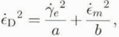
Duva and Crow’s model involves a viscoplastic potential which, at a fixed density, depends on a single invariant σ D of the strain rates given by
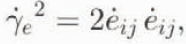
where  is the second invariant of the deviatoric strain rates defined as
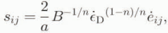
and a and b are functions of the material density only. With this notation, the stresses are expressed in terms of strain rates by the following relations:


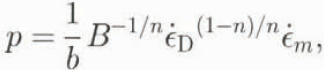
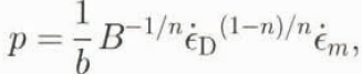
the inversion of which gives
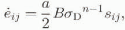
and

where σ D is the stress invariant defined by
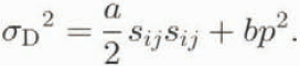
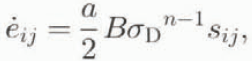
From Equations (8) and (10) we obtain
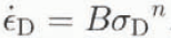
The behaviour of an incompressible material is obtained for a = 1 and b = 0. In this case Ĕ m = 0, Ĕ ij, Equation (12) is the usual Glen’s law (with Ĕ D =  =
 and σ D = τ), and Equations (7) and (9) reduce to Norton-Holf power law which is the multiaxial extension of Glen’s law, generally used to describe the behaviour of isotropie glacier ice.
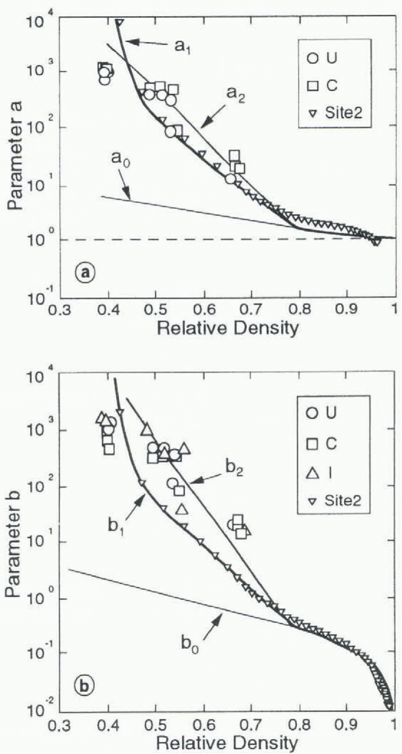
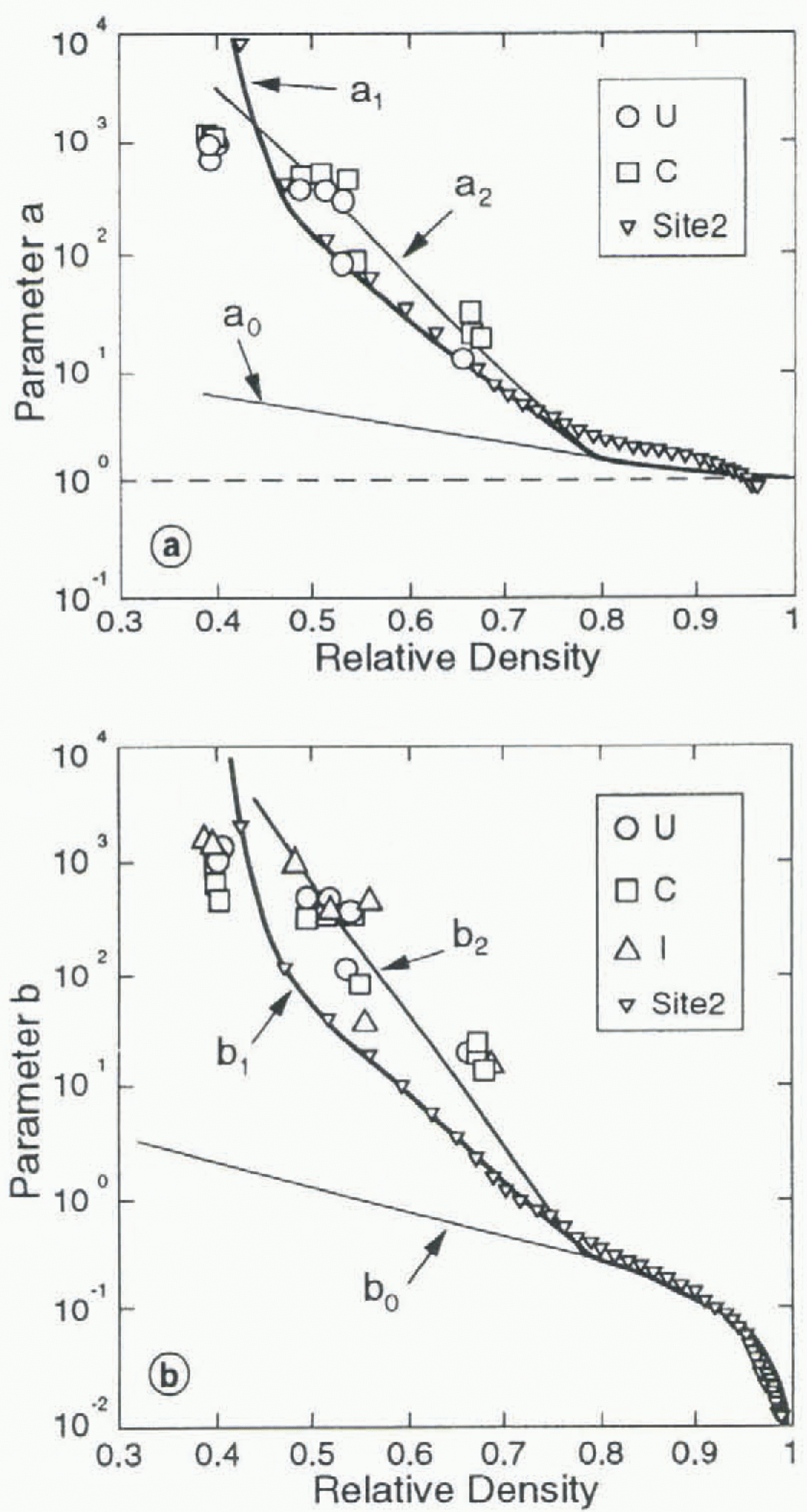
Model parameters a (a) and b (b) vs relative density D. Solid lines show Duva and Crow’s (1994) original functions (a0, b), and functions (a1, b2), (a2, b2) used in this study. Symbols show the values corresponding to Site 2 data and to Landauer’s (1957) creep tests (U, uniaxial compression; C, confined compression; I, isotropic compression).
Application to firn and ice
Duva and Crow’s (1994) expressions for the density dependence of functions a and b are a = a 0 and b = b 0 with:
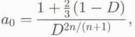
and
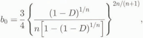
where D is the relative density (or solid volume fraction) of the material. For porous ice D = ρ/ρ ice where ρ is the actual firn density, and ρ ice = 0.917 Mg m–1 is the density of pure ice.
According to Duva and Crow (1994), Equation (14) leads to a densification rate, under isotropie pressure, equivalent to that given by Wilkinson and Ashby’s (1975) spherical-pore model. This latter model was shown by Pimienta (1987) to correctly reproduce the densification of polar ice for D > 0.785. According to Duval (1985), cold firn densification at lower densities is driven by grain rearrangement, compaction and diffusion for D < 0.6, then by dislocation creep in the contact areas until pore close-off occurs. Within this density range, Equations (13) and (14) are not valid.
To obtain an estimate of functions a and b which can be relevant for our study (0.4 < D < 1), we used the data of Site 2, Greenland (Langway, 1967) where the horizontal velocity can be neglected (unlike at Dôme du Goûter). Assuming that densification occurs under vertical compression without lateral displacement (i.e. Ĕ x = Ĕ y = 0, and σ z resulting from the supcrimposed-ice column), it was possible to compute the values of a and b which allow reproduction of the measured densities corresponding to the observed surface accumulation rate, under the condition that a/b remains equal to a //bb. The discrete values of a and b obtained by solving this inverse problem are shown in figure 2a and b. A continuous representation, noted a 1 and b 1, suitable for numerical computations, was obtained as:
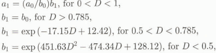
where a 0 and b 0 are given by Equations (13) and (14). The corresponding curves are drawn in figure 2a and b.
In order to assess the influence of a and b on the simulation, another set of functions, noted a 2 and b 2, was obtained by analysing the experimental results of Landauer (1957) through Duva and Crow’s (1994) model. Landauer performed a number of creep tests on snow, under isotropic compression, uniaxial compression and compression with lateral confinement, and found that for relative densities D between 0.39 and 0.69, and loads between 0.027 and 0.27 MPa, the appropriate value of exponent n was 3. The corresponding values of a and b are shown in figure 2a and b, as well as the continuous set of functions which fit these values, given by:
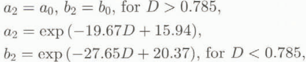
where a 0 and b 0 are given by Equations (13) and (14).
Other experimental studies (Bader and others, 1955; Mellor and Hendrickson, 1965; Kojima, 1974; Desrues and others, 1980) could not be used, sometimes because of missing test conditions, and generally owing to the big changes in density during the tests.
Numerical Simulation
Variational formulation of the flow problem
For a given field of relative density, with D strictly less than 1 everywhere, (i.e. b > 0), the solution of the flow problem in domain V minimizes, among all admissible velocity fields (Hill’s minimum principle):

where the dissipation potential ФE is given by

u i, g i are the velocity and gravity forces components, and Г denotes the boundary of V where the stress vector, of components Σi, is prescribed.
This formulation, used by Duva and Crow (1994), is not suited for our problem since we have to deal with both compressible firn and incompressible ice. To overcome this difficulty we adopted a mixed (velocity-pressure) formulation, based on the application of the virtual work principle, in which compressibility Equation (8) is enforced by using the pressure as a Lagrange multiplier. Among all admissible velocity fields, the solution of the flow problem is such that
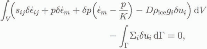
where
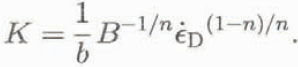
When the relative density is equal to 1 (b = 0, 1/K = 0), this formulation is fully equivalent to that employed to simulate the flow of incompressible ice (Meyssonnier, 1989).
From a technical point of view, the solution of the functional Equation (19) was achieved by the finite-element method, using six-node triangular elements with a quadratic interpolation of the velocities and a linear interpolation of the pressure (see Meyssonnier, 1989). The relative densities were given as quadratic functions of the coordinates as well. The computation was done under the assumption of axisymmetric flow.
Formulation of the densification problem
For a given velocity field, and under the assumption of stationarity, the Eulerian description of the densification problem is given by the equation ∂D/∂t = 0, that is:
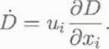
Following a given mass of porous ice along its trajectory, its density variation is induced by the change in volume so that
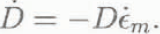
The solution of the densification problem is then obtained by solving the equation

In order to keep some homogeneity in the treatment of the model by using finite-element technique, we attempted to solve Equation (23) by Galerkin’s method (Agrawal and Dawson, 1985; Chenot and others, 1990) and by a least-squares procedure (Kanarachos, 1982). The former turned out to be very unstable (owing to the large variation in D from surface to bedrock), and the latter resulted in a too efficient smoothing of the relative density.
The efficient, but computation-time consuming, procedure which was adopted consists in solving Equation (23) along the flow streamlines. Denoting by S the curvilinear coordinate along a streamline (not to be confused with the deviatoric stress tensor s), and by u s the velocity tangent to this streamline, Equation (23) transforms into:
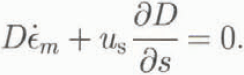
The relative density at each node M of the finite-element mesh was computed in the following manner: the streamline arriving at M was computed from M to the glacier surface (using the previous velocity field obtained by finite-element computation) by solving the set of equations dx i/dt = –u i (upstream procedure); in parallel, Equation (24) was solved by a Runge–Kutta method.
Boundary conditions
The only boundary condition needed for the densification problem is the surface density ρ which was set to 0.4 Mg m–3, independently of the position. For the flow problem, the simple boundary conditions adopted were no sliding at the glacier/bedrock interface (the ice temperature is –11∘C) and a stress-free surface (doing so, the computed surface velocities serve as control for the simulation). The condition to be prescribed at the downstream (fictitious) boundary of the flow domain is not obvious since the topographic measurements ended about 100 m downstream from the borehole locations. To minimize the effects of this condition on the glacier flow in the vicinity of the boreholes, the studied domain was extended downstream by a 100 m (Fictitious) outer ring (see marks A and B in Figure 1). Thus the lateral boundary of the axisymmetric model is placed at r = 500 m, r being the radial coordinate. Two types of boundary condition, noted BC1 and BC2, were tried: BC1 assumes that the lateral boundary is stress-free; BC2 is a kinematic condition which assumes that the vertical velocity w and the relative density D are independent of r, and that the horizontal velocity u verifies mass conservation, that is δw/δr = 0 and δ(ur)/δr = 0.
Problem coupling
The simulation was processed by solving the non-linear flow problem (Equations (19), (7) and (20)) for a given density field, then the densification problem (Equation (24)) for a given velocity field. The initial density field was derived from Herron and Langway’s (1980) model. Special attention was needed to solve the densification problem, in order to prevent instabilities and unphysical results (i.e. relative densities greater than 1), which could arise during intermediate steps of the computation. To avoid problems with streamlines possibly intersecting the bedrock (a situation that can be encountered when the overall density is too low), the density was set to D = 1 at the first layer of nodes close to the bedrock, allowing a possible discontinuity of D at the top of this layer. As regards the axis of symmetry (r = 0), which is a particular streamline, the densities were left at their initial value. To ensure a smooth convergence of the coupled problem, a relaxation factor was introduced to limit the density variations from step to step. D * being the density solution of Equation (24), corresponding to the velocities computed at step i with D i, the density at step i + 1 was taken (at each node) as:

with 0 < k < 0.1. If a nodal density D * was found to be greater than I, it was replaced with 1 in Equation (25).
The procedure was repeated until convergence was achieved for both velocity and density fields.
Results And Discussion
All the computations were done using the same regular mesh (part of which is shown in Figure 1). Exponent n in Equations (7)–(14) was given the standard value of 3. Taking into account the nature of the boundary conditions prescribed,
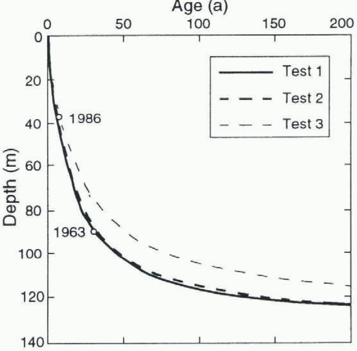
Age of the ice vs depth in borehole 2. Radioactive levels are shown by circles. For tests 1 and 2 curves were computed with B = 20 MPa–3 a–1. Test 3 curve for B = 20 MPa–3 a–1 is shown for comparison. (Test 3 curve for B = 31 MPa–3 a–1, not shown, is superposed on test l and 2 curves).
Glen’s law parameter B only plays the role of a scaling parameter for the velocities (relative densities are not affected by the value of B). Its value was set arbitrarily at 5 MPa–3 a–1 in order to perform the computations with a reasonable order of magnitude of the velocities.
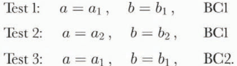
Three sets of results, tests 1, 2 and 3, are presented. They were achieved by using expressions (a 1, b 1) or (a 2, b 2), given by Equations (15) and (16), respectively, for functions a and b, and by prescribing the lateral boundary condition as BC1 or BC2, namely:
Glen’s law parameter B
The final value of B was adjusted for each test so that the age of the ice particle which reaches the 1963 radioactive level, in borehole 2, was correct. The computed velocity field was scaled consequently. The corresponding values for tests 1 and 2 were B=20 MPa–3 a–1, while for test 3 the correct age of the ice was obtained with B = 31 MPa–3 a–1. Meyssonnier and Gouberťs (1994) experiments lead to a value of B close to 17 MPa–3 a–1 at –10∘C, corresponding to the minimum creep rate (secondary creep). Lliboutry and Duval (1985) adopt the values B = 19 MPa–3 a–1 for secondary creep at –10°C, with an activation energy Q = 76.5 KJ mol–1. Following these authors, the corresponding temperatures would be –9.5∘C for tests 1 and 2, and –6∘C for test 3. Then, as the in situ measured temperature varies between –9∘ and –11∘C, the values of B found in our simulations are not unrealistic. However, owing to the fact that a volume of ice travelling from the glacier surface to the bedrock experiences transient, then secondary and possibly tertiary creep, which is not taken into account by the rheological model used in this study, the values of B derived from the simulation are only mean values. Since the value of B for tertiary creep is about 250 MPa–3 a–1 at 0∘C (Lliboutry and Duval, 1985; Meyssonnier, 1989), which gives B = 70 MPa–3 a–1 at –10∘C, the differences found in the three tests do not allow one of them to be selected as the most relevant.
The age of the ice vs depth along the borehole 2 vertical, computed with the same value B = 20 MPa–3 a–1 for the three tests, is shown in Figure 3. The test 3 curve computed with B = 31 MPa–3 a–1, not shown in the figure, is superposed on the test 1 and 2 curves. Thus the age of the ice seems tobe independent of the test conditions.
Velocities
Velocity profiles along a vertical resulting from the three tests exhibit the same shape, an example of which is shown in Figure 1. For the same value of B, the magnitude of the velocity is greater in tests 1 and 2 than in test 3, owing to the stress-free lateral boundary condition. As a consequence of this condition, the velocity fields achieved in tests 1 and 2 are quite unrealistic in the region near the border of the flow domain (r > 400 m; section A–B on Figure 1). The computed streamlines (test 1) are shown on Figure 1. Note that, except the symmetry axis of the model, none of them intersect
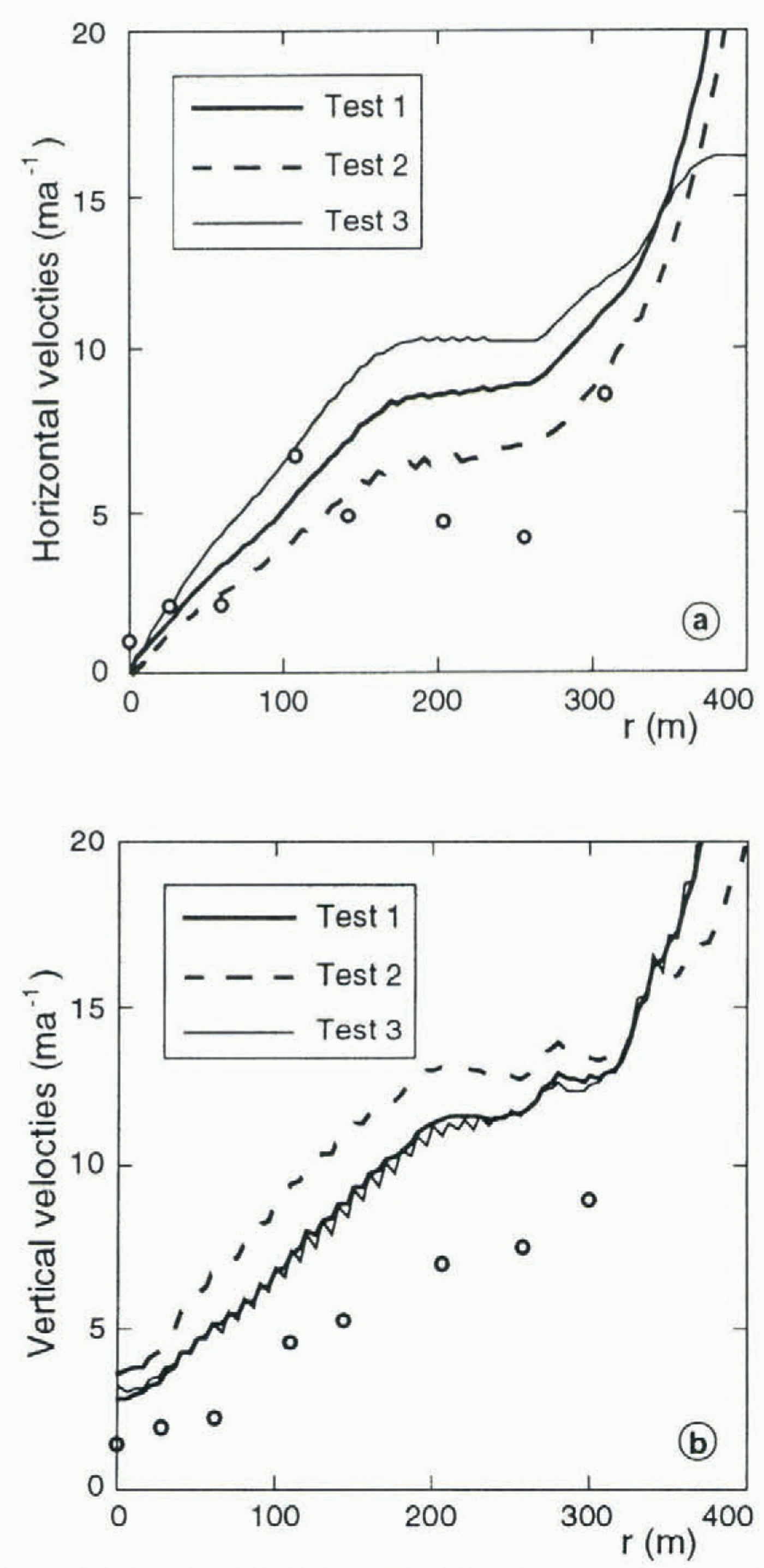
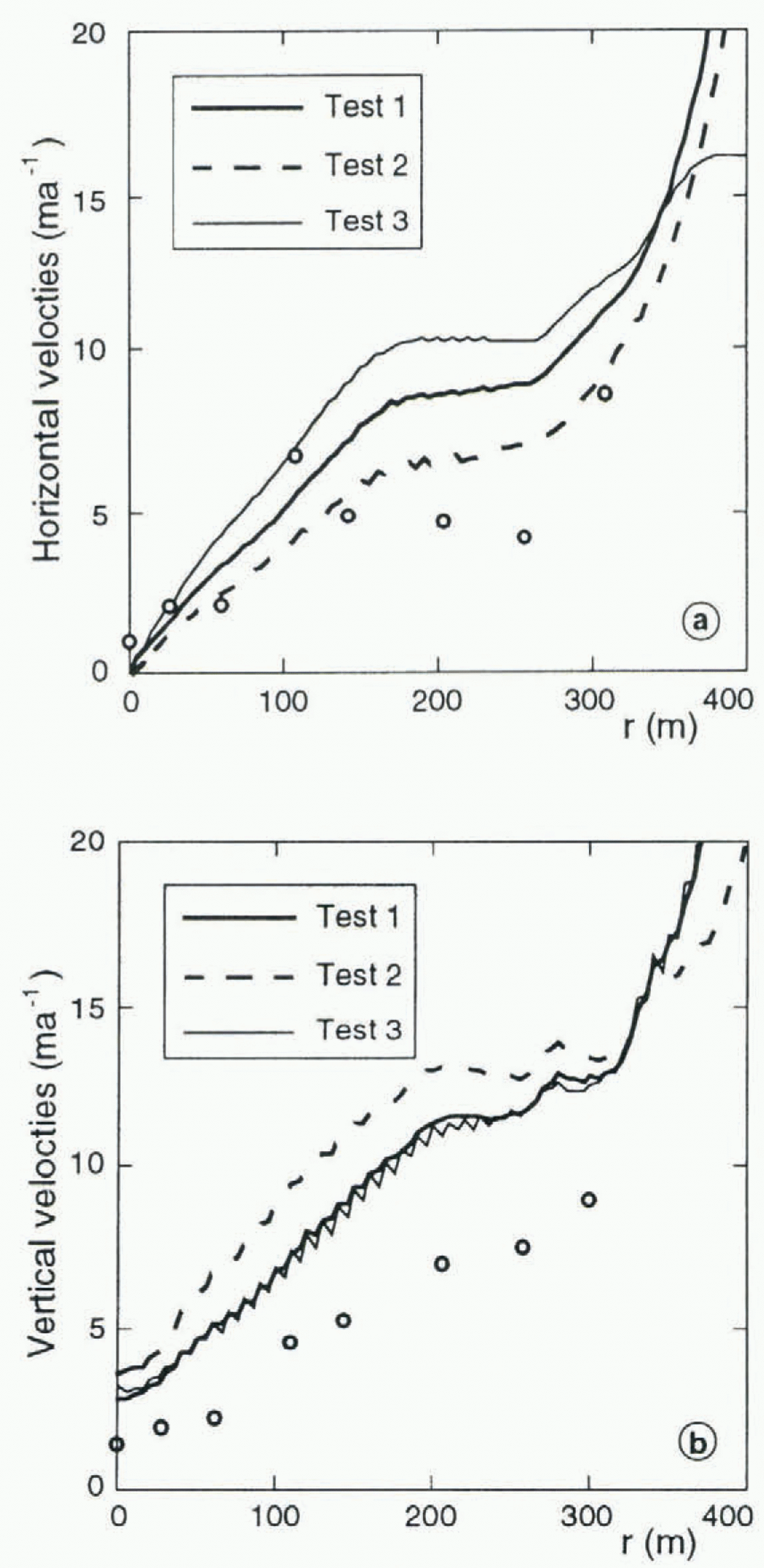
Horizontal (a) and vertical (b) surface velocities computed with B = 20 MPa–3 a–1 for tests 1 and 2, and B = 31 MPa–3 a–1 for test 3. The measured velocities are shown by circles.
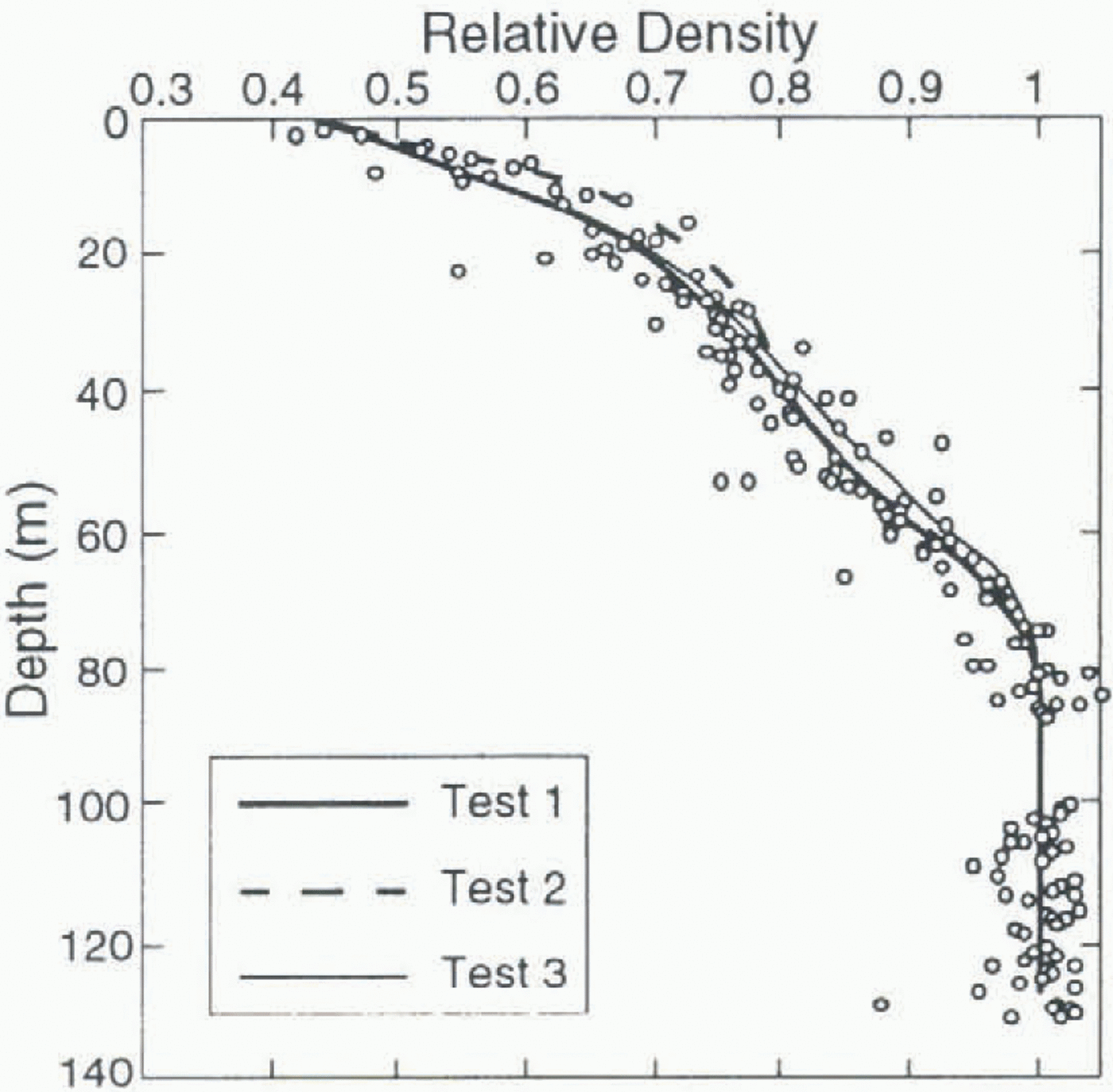
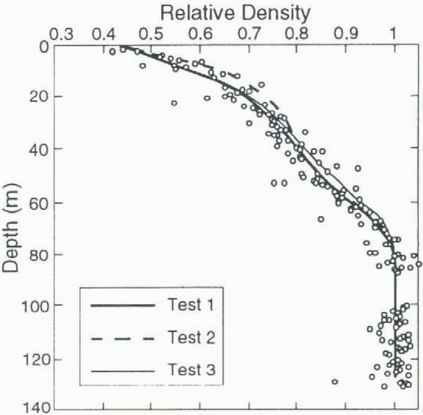
Relative density profile along the borehole 2 ice core. The computed profiles are shown by solid and dashed lines. Measured values are shown by circles.
the bedrock. This is quite a reasonable result, which is an indication that the computed density field is consistent with the assumption of stationary flow.
The horizontal and vertical velocities along the glacier surface are shown in figure 4a and b. These curves were drawn with B = 20 MPa–3 a–1 for tests 1 and 2, and B = 31 MPa–3 a–1 for test 3. In tests 1 and 3, vertical velocities (Fig. 4b) are almost identical, while test 2 exhibits higher values. This is explained by the higher value of b for this test, and by the fact that snow compaction has a major influence on the vertical velocity at the glacier surface. On the contrary, the surface horizontal velocity is mainly influenced by the value of a which controls the shear strain rate. Test 2 horizontal velocities are smaller than those of test 1 (see Fig. 4a) because a 2 is smaller than a 1 at the surface density D < 0.45 (see Fig. 2a). In general, the magnitude of the surface velocity is higher (by a factor of about 2) than the accumulation rate and than the measured velocity, in all tests. This may be caused by too high values of both a and b at low densities, or by the fact that the Dôme du Gûter is not in a stationary state.
Densities
The computed density contours look very similar in the three tests, except near the lateral boundary where the stress-free condition of tests 1 and 2 generates higher vertical velocities. They give the image of a layered medium, as expected. The region D > 0.99 (nearly the same for all tests) is shown in Figure 1 (shaded area).
The computed density profile along the borehole 2 vertical is shown in Figure 5, together with the density measured along the ice core. In the range 0.4 < D < 0.785, test 2 results in a density gradient higher than that obtained in test 1, owing to the fact that b 2 is greater than b 1, giving a higher compaction rate. This influence is only noticeable in the 30 m below the surface, past which the density profiles are identical. The difference in the lateral boundary condition (see Fig. 5, tests 1 and 3) has no effect near the glacier surface, and a very small one for D > 0.7. The measured density profile is generally well represented by the simulations, with a slight advantage for tests 1 and 3. Note that the simulated density profiles do not depend on the value of Glen’s law parameter B.
Conclusion
A flow simulation of the cold glacier of Dôme du Goûter has been presented. We made use of a special rheological model to describe the behaviour of firn and ice, adapted from the literature on the basis of polar firn-densification data and of creep-test results on snow, that is irrespective of the Dôme du Goûter available data. The finite-element formulation adopted to solve the flow problem allows passage from firn to ice in a continuous manner. The use of this model for glacier-flow simulation with this formulation constitutes the main interest and originality of the study.
The simulation was based on the assumption of stationary state, but the computed surface velocities were found to be much higher than that observed. On the other hand, the measured density profile is very well reproduced by the model. No straightforward conclusion can be drawn as regards the stationarity of the glacier, as surface velocities are extremely sensitive to the values of rheological parameters a and b at low densities. As these parameters certainly do not depend only on the density but also on the actual structure of snow, a more detailed study of snow behaviour at the glacier surface should be done in order to check their order of magnitude.
The ages of the ice along the ice-core, computed with different sets of functions a and b and different lateral boundary conditions, are in accordance. An age of 120 a is found at 120 m depth, past which the asymptotic shape of the date curve renders any prediction meaningless.
Acknowledgements
We thank L. Reynaud, M. Funk, M. Pourchet, F. Pinglot and C. Vincent, who provided us with a great amount of field data along with very helpful comments and discussion. Special thanks are due to an anonymous referee who generously gave his time to improve the quality of our English.