1 Introduction
In this paper, we examine the motion of a droplet with an interface whose mechanics cannot be solely described by surface tension. Multiple examples of such systems exist in biological and industrial applications, such as capsules (Discher et al. Reference Discher, Won, Ege, Lee, Bates, Discher and Hammer1999; Lee & Feijen Reference Lee and Feijen2012; Barthés-Biesel Reference Barthés-Biesel2016), vesicles (Abreu et al. Reference Abreu, Levant, Steinberg and Seifert2014; Narsimhan, Spann & Shaqfeh Reference Narsimhan, Spann and Shaqfeh2014; Dahl et al. Reference Dahl, Narsimhan, Gouveia, Kumar, Shaqfeh and Muller2016; Vlahovska, Podgorski & Misbah Reference Vlahovska, Podgorski and Misbah2009b ) and solid-stabilized foams/emulsions (Langevin Reference Langevin2000; Cates & Clegg Reference Cates and Clegg2008; Velikov & Velev Reference Velikov and Velev2014). Here, we focus on a specific system where the interface has a large degree of viscous dissipation – i.e. surface viscosity. This situation arises in emulsions when a droplet has a concentrated layer of insoluble surfactant, fatty acid, or polymer on its surface (Erni Reference Erni2011; Fuller & Vermant Reference Fuller and Vermant2012). The interfacial stresses generated play an important role in the stability of emulsions and foams, and thus there has been a lot of interest in developing experimental methods to measure the interfacial viscosities of such surfaces (Brooks et al. Reference Brooks, Fuller, Frank and Robertson1999; Choi et al. Reference Choi, Steltenkamp, Zasadzinski and Squires2011). The goal of this paper is to investigate the role that interfacial viscosity plays on the shape of a single droplet in flow, as well as the nonlinear rheology of a bulk suspension of droplets. The perturbation theories developed here can also provide insight into droplet breakup, which will be discussed a bit in this paper and further expanded in a future publication.
The simplest model that describes the mechanics of an interface with viscous dissipation is the Boussinesq–Scriven law (Boussinesq Reference Boussinesq1913; Scriven Reference Scriven1960), which treats the droplet surface as a homogeneous fluid with a two-dimensional (2D) shear and dilational viscosity. Under this model, several papers have investigated the motion and deformation of droplets under various flows. Levan (Reference Levan1981) described how interfacial viscosity alters the translational speed of droplets under an external force, and others described droplet motion under dielectrophoresis (Mandal & Chakraborty Reference Mandal and Chakraborty2017), thermophoresis (Levan Reference Levan1981), and an external pressure gradient (Schwalbe et al. Reference Schwalbe, Phelan, Vlahovska and Hudson2011), all of which was summarized succinctly in an article by Narsimhan (Reference Narsimhan2018). The effect of non-uniform surface viscosities on droplet translation has been explored by Manor, Lavrenteva & Nir (Reference Manor, Lavrenteva and Nir2008). For droplet deformation, Flumerfelt (Reference Flumerfelt1980) developed perturbation theories to describe the shape of droplets with surface viscosities in weak shear flows, similar to the classical theories of Cox (Reference Cox1969) for a clean droplet. These theories do not go beyond the lowest-order deformation, and hence cannot extract information about nonlinear rheology or breakup. LeVan and Flumerfelt’s theories were later investigated in experiments as possible methods to measure surface rheological properties (Phillips, Graves & Flumerfelt Reference Phillips, Graves and Flumerfelt1980; Erk et al. Reference Erk, Martin, Schwalbe, Phelan and Hudson2012).
Most simulations of droplets with a viscous surface investigate the role of interfacial viscosity on the shape of droplets, looking beyond the range of validity afforded by Flumerfelt’s theory (Pozrikidis Reference Pozrikidis1994; Gounley et al. Reference Gounley, Boedec, Jaeger and Leonetti2016). However, there is still a significant discrepancy between the boundary element simulations and perturbation theories in describing the droplet orientation, which this manuscript addresses. Outside of standard droplets, interfacial viscosity has been found to be important in many areas of bio-inspired science. For example, Saffman & Delbrück (Reference Saffman and Delbrück1975) noted that the surface viscosity of lipid bilayers plays a major role in describing the transport and dynamics of molecules, proteins, and lipid rafts in cellular membranes (Klingler & McConnell Reference Klingler and McConnell1993; Cicuta, Keller & Veatch Reference Cicuta, Keller and Veatch2007). Surface viscosity can explain anomalous (logarithmic) scaling of the diffusion constant of globular proteins with protein size, an area that is under significant investigation today (Gambin et al. Reference Gambin, Lopez-Esparza, Reffay, Sierecki, Gov, Genest, Hodges and Urbach2006; Brown Reference Brown2011). We note that the growth rate of vesicle pearling (Narsimhan, Spann & Shaqfeh Reference Narsimhan, Spann and Shaqfeh2015) as well as the tank treading of capsules/red blood cells (Bagchi & Kalluri Reference Bagchi and Kalluri2010) are both altered by the presence of membrane dissipation. For synthetic capsules, some of which are used in drug delivery, interfacial viscosity appears to explain some of the discrepancy between experiments (de Loubens et al. Reference de Loubens, Deschamps, Edwards-Levy and Leonetti2016) and theory (Barthés-Biesel & Sgaier Reference Barthés-Biesel and Sgaier1985) in describing their deformation in flow. Although important, we note that spherical capsules have different interfacial mechanics than droplets, where surface tension effects are essential.
Currently, we are unaware of analytical theories that examine how interfacial viscosity alters the nonlinear rheology of droplet emulsions and droplet breakup. To answer these questions, we are motivated by the studies of Barthés-Biesel & Acrivos (Reference Barthés-Biesel and Acrivos1973), as well as Rallison (Reference Rallison1980), who developed perturbation theories of droplet shape evolution/breakup for clean droplets in the limit of small deformation. We perform the same methods here but now include interfacial rheology, which allows us to examine how these effects alter droplet deformation and stress. Section 2 outlines the problem set-up and solution methodology. Section 3 summarizes the general equations we obtain for droplet shape and suspension stress in a linear flow field. We derive expressions for two different scenarios: (i) small capillary number (weak flow), and (ii) large viscous resistance, which corresponds to large surface viscosities or large interior droplet viscosity. Section 4 summarizes major results for droplet shape in shear and extensional flows, both under steady-state and transient dynamics. Our results improve upon the original small-deformation theories of Flumerfelt (Reference Flumerfelt1980), and resolve the discrepancies between analytical theories and boundary element simulations (Gounley et al. Reference Gounley, Boedec, Jaeger and Leonetti2016). The theories developed here also accurately quantify the inclination angle of clean drops over a larger range of viscosity ratios and capillary numbers than previous works (Chaffey & Brenner Reference Chaffey and Brenner1967; Cox Reference Cox1969), which is a valuable development in its own right. Section 5 calculates the nonlinear rheology of a dilute suspension of droplets, quantifying shear thinning, extensional thickening and normal stress differences. The normal stress differences are intimately related to the droplet migration in wall-bound shear flow (Smart & Leighton Jr Reference Smart and Leighton1991), and we discuss the consequence of shear/dilational viscosity on this motion. Section 6 concludes by discussing how our theories can be extended to more complicated situations, such as when droplets have a viscoelastic membrane and/or Marangoni flows. We also discuss how one can derive theories of droplet breakup using the shape evolution equations developed in this paper.
2 Problem overview and methodology
2.1 Problem statement and non-dimensionalization
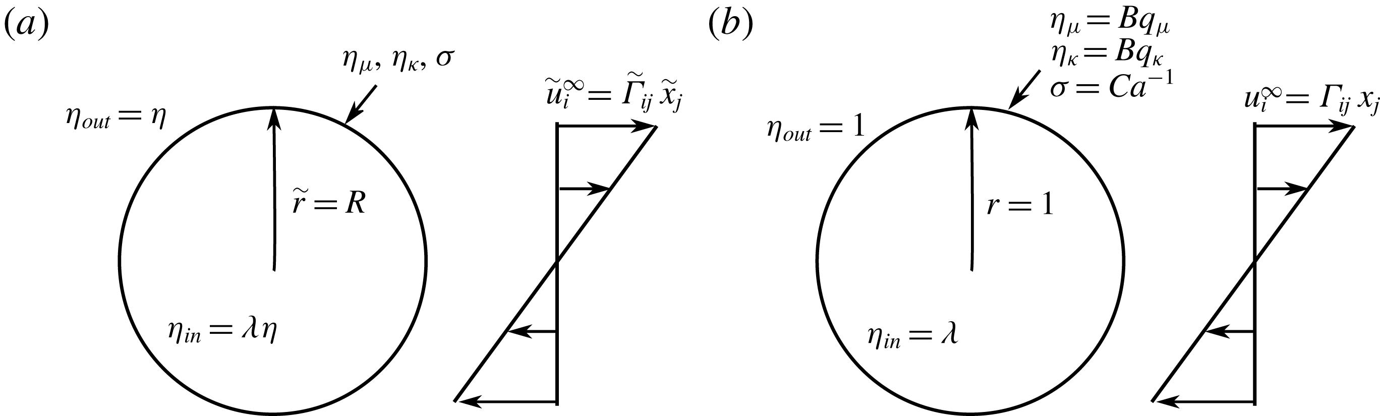
Problem set-up. (a) Dimensional quantities. (b) Dimensionless quantities.

Figure 1 shows the problem set-up. A droplet of radius
 $R$
and viscosity
 $\unicode[STIX]{x1D706}\unicode[STIX]{x1D702}$
is placed in a fluid of viscosity
 $\unicode[STIX]{x1D702}$
. On the droplet’s surface is a thin layer of insoluble, surface-active agents with interfacial viscosities
 $\unicode[STIX]{x1D702}_{\unicode[STIX]{x1D707}}$
and
 $\unicode[STIX]{x1D702}_{\unicode[STIX]{x1D705}}$
, where
 $\unicode[STIX]{x1D702}_{\unicode[STIX]{x1D707}}$
is the surface shear viscosity and
 $\unicode[STIX]{x1D702}_{\unicode[STIX]{x1D705}}$
is the surface dilational viscosity. The surface tension of the clean interface is
 $\unicode[STIX]{x1D70E}$
. We would like to know how the surface moduli
 $\unicode[STIX]{x1D702}_{\unicode[STIX]{x1D707}}$
and
 $\unicode[STIX]{x1D702}_{\unicode[STIX]{x1D707}}$
alter the dynamics of the droplet when placed in a linear velocity field
 $\tilde{u} _{i}^{\infty }=\tilde{\unicode[STIX]{x1D6E4}}_{ij}\tilde{x}_{j}$
, where
 $\tilde{\unicode[STIX]{x1D6E4}}_{ij}$
is the far-field velocity gradient with characteristic magnitude
 $\dot{\unicode[STIX]{x1D6FE}}=|\tilde{\unicode[STIX]{x1D6E4}}_{ij}|$
(note: repeated indices are summed unless otherwise stated). We examine this problem in the creeping flow limit (i.e. Stokes flow) and the small-deformation regime. The latter occurs when the capillary number
 $Ca=\unicode[STIX]{x1D702}\dot{\unicode[STIX]{x1D6FE}}R/\unicode[STIX]{x1D70E}\ll 1$
, or when the viscous resistance of the droplet is large (i.e.
 $\unicode[STIX]{x1D706}\gg 1$
or
 $\unicode[STIX]{x1D702}_{\unicode[STIX]{x1D707}}\gg R\unicode[STIX]{x1D702}$
). In this analysis, we assume a constant surface tension
 $\unicode[STIX]{x1D70E}$
, although in actuality surfactants can be mobile and introduce Marangoni flows (i.e. surface tension inhomogeneities). If the Marangoni flows are weak and surface convection negligible, one can incorporate these effects into an apparent dilational viscosity, as illustrated in appendix A. At the end of the paper, we discuss how to extend aspects of our model to more complicated situations (stronger Marangoni flows and/or viscoelastic surfaces).
From here on out, we non-dimensionalize all lengths by the droplet radius
 $R$
, times by a capillary time scale
 $t_{c}=\unicode[STIX]{x1D702}R/\unicode[STIX]{x1D70E}$
, velocities by
 $\dot{\unicode[STIX]{x1D6FE}}R$
, stresses by
 $\unicode[STIX]{x1D702}\dot{\unicode[STIX]{x1D6FE}}$
, and surface stresses by
 $\unicode[STIX]{x1D702}R\dot{\unicode[STIX]{x1D6FE}}$
. Dimensional quantities have a tilde, while non-dimensional quantities do not:
 $$\begin{eqnarray}x_{i}={\displaystyle \frac{1}{R}}\tilde{x}_{i},\quad t={\displaystyle \frac{\unicode[STIX]{x1D70E}}{\unicode[STIX]{x1D702}R}}\tilde{t}\quad u_{i}={\displaystyle \frac{1}{\dot{\unicode[STIX]{x1D6FE}}R}}\tilde{u} _{i},\quad \unicode[STIX]{x1D70F}_{ij}={\displaystyle \frac{1}{\dot{\unicode[STIX]{x1D6FE}}\unicode[STIX]{x1D702}}}\tilde{\unicode[STIX]{x1D70F}}_{ij}\quad \unicode[STIX]{x1D70F}_{ij}^{s}={\displaystyle \frac{1}{\dot{\unicode[STIX]{x1D6FE}}\unicode[STIX]{x1D702}R}}\tilde{\unicode[STIX]{x1D70F}}_{ij}^{s}.\end{eqnarray}$$
We also decompose the velocity gradient into a symmetric rate-of-strain tensor
 $\unicode[STIX]{x1D60C}_{ij}$
and an antisymmetric rate-of-rotation tensor
 $\unicode[STIX]{x1D6FA}_{ij}$
.
 $$\begin{eqnarray}\unicode[STIX]{x1D6E4}_{ij}=\unicode[STIX]{x1D60C}_{ij}+\unicode[STIX]{x1D6FA}_{ij}\quad \unicode[STIX]{x1D60C}_{ij}={\textstyle \frac{1}{2}}(\unicode[STIX]{x1D6E4}_{ij}+\unicode[STIX]{x1D6E4}_{ji})\quad \unicode[STIX]{x1D6FA}_{ij}={\textstyle \frac{1}{2}}(\unicode[STIX]{x1D6E4}_{ij}-\unicode[STIX]{x1D6E4}_{ji}).\end{eqnarray}$$
In this problem, there are four dimensionless quantities that govern the droplet dynamics:
(i) The viscosity ratio between interior and exterior fluid
 $\unicode[STIX]{x1D706}$
.
(ii) The capillary number
$Ca\equiv \unicode[STIX]{x1D702}\dot{\unicode[STIX]{x1D6FE}}R/\unicode[STIX]{x1D70E}$
.(iii) The Boussinesq number
$Bq_{\unicode[STIX]{x1D707}}=\unicode[STIX]{x1D702}_{\unicode[STIX]{x1D707}}/(R\unicode[STIX]{x1D702})$
for surface shear viscosity.(iv) The Boussinesq number
$Bq_{\unicode[STIX]{x1D705}}=\unicode[STIX]{x1D702}_{\unicode[STIX]{x1D705}}/(R\unicode[STIX]{x1D702})$
for surface dilational viscosity.


The Boussinesq numbers examine the relative contribution of the surface to bulk viscosities on the droplet dynamics. In this manuscript, we discuss two regimes where the droplet deformation is small: (i) weak flow, where
 $Ca\ll 1$
and
 $\unicode[STIX]{x1D706}$
,
 $Bq_{\unicode[STIX]{x1D707}}$
and
 $Bq_{\unicode[STIX]{x1D705}}\sim O(1)$
, and (ii) strong viscous resistance, where
 $Ca\sim O(1)$
and
 $\unicode[STIX]{x1D706}\gg 1$
, or
 $Ca\sim O(1)$
and
 $Bq_{\unicode[STIX]{x1D705}}\sim Bq_{\unicode[STIX]{x1D707}}\gg 1$
. For illustrative purposes, we discuss the weak flow case (
 $Ca\ll 1$
) in the methodology below. Section 3 discusses how to extend the methodology to
 $\unicode[STIX]{x1D706}\gg 1$
or
 $Bq_{\unicode[STIX]{x1D705}}\sim Bq_{\unicode[STIX]{x1D707}}\gg 1$
, and §§ 4–5 discusses major results for all cases.
2.2 Governing equations
We follow the methodology of Barthés-Biesel & Acrivos (Reference Barthés-Biesel and Acrivos1973) and Rallison (Reference Rallison1980), only highlighting the major parts of their analysis. We solve the Stokes equations for velocity and pressure:
 $$\begin{eqnarray}\unicode[STIX]{x1D6FB}^{2}u_{i}=\unicode[STIX]{x1D707}{\displaystyle \frac{\unicode[STIX]{x2202}p}{\unicode[STIX]{x2202}x_{i}}};\quad {\displaystyle \frac{\unicode[STIX]{x2202}u_{i}}{\unicode[STIX]{x2202}x_{i}}}=0,\end{eqnarray}$$
where
 $\unicode[STIX]{x1D707}$
is the non-dimensional viscosity of the fluid, equalling
 $\unicode[STIX]{x1D707}=1$
outside the droplet and
 $\unicode[STIX]{x1D707}=\unicode[STIX]{x1D706}$
inside the droplet. These equations are subject to the following boundary conditions: (i) far-field velocity:
 $u_{i}\rightarrow \unicode[STIX]{x1D6E4}_{ij}x_{j}$
as
 $|x_{i}x_{i}|\rightarrow \infty$
, (ii) continuity of velocity across the droplet surface:
 $[[u_{i}]]=0$
, and (iii) force balance across the droplet surface:
 $[[\unicode[STIX]{x1D70F}_{ij}n_{j}]]=\unicode[STIX]{x2202}(\unicode[STIX]{x1D6F4}_{ij}^{S})/\unicode[STIX]{x2202}x_{j}^{S}$
. For these expressions,
 $[[\cdots ]]$
represents a jump across the interface, i.e.
 $[[g]]=g_{out}-g_{in}$
. In the force balance condition,
 $\unicode[STIX]{x1D70F}_{ij}$
is the Newtonian stress tensor,
 $n_{i}$
is the outward-pointing normal vector, and
 $\unicode[STIX]{x2202}/\unicode[STIX]{x2202}x_{i}^{S}$
is the surface gradient operator, defined as
 $\unicode[STIX]{x2202}/\unicode[STIX]{x2202}x_{i}^{S}=\unicode[STIX]{x1D617}_{ik}\unicode[STIX]{x2202}/\unicode[STIX]{x2202}x_{k}$
, where
 $\unicode[STIX]{x1D617}_{ij}=\unicode[STIX]{x1D6FF}_{ij}-n_{i}n_{j}$
is projection operator on the surface. The quantity
 $\unicode[STIX]{x1D6F4}_{ij}^{\unicode[STIX]{x1D61A}}$
is the surface stress tensor, which has contributions from surface tension, surface shear viscosity and surface dilational viscosity. We write the three contributions below:
 $$\begin{eqnarray}\displaystyle & \displaystyle \unicode[STIX]{x1D6F4}_{ij}^{S,\unicode[STIX]{x1D70E}}=-{\displaystyle \frac{1}{Ca}}\unicode[STIX]{x1D617}_{ij}, & \displaystyle\end{eqnarray}$$
 $$\begin{eqnarray}\displaystyle & \displaystyle \unicode[STIX]{x1D6F4}_{ij}^{S,\unicode[STIX]{x1D707}}=Bq_{\unicode[STIX]{x1D707}}\left[\unicode[STIX]{x1D617}_{ij}{\displaystyle \frac{\unicode[STIX]{x2202}u_{m}}{\unicode[STIX]{x2202}x_{m}^{S}}}-\unicode[STIX]{x1D617}_{ik}\left({\displaystyle \frac{\unicode[STIX]{x2202}u_{n}}{\unicode[STIX]{x2202}x_{k}^{S}}}+{\displaystyle \frac{\unicode[STIX]{x2202}u_{k}}{\unicode[STIX]{x2202}x_{n}^{S}}}\right)\unicode[STIX]{x1D617}_{nj}\right], & \displaystyle\end{eqnarray}$$
 $$\begin{eqnarray}\displaystyle & \displaystyle \unicode[STIX]{x1D6F4}_{ij}^{S,\unicode[STIX]{x1D705}}=-Bq_{\unicode[STIX]{x1D705}}\left[\unicode[STIX]{x1D617}_{ij}{\displaystyle \frac{\unicode[STIX]{x2202}u_{m}}{\unicode[STIX]{x2202}x_{m}^{S}}}\right]. & \displaystyle\end{eqnarray}$$
So far, the set-up of the problem is exactly the same as Barthés-Biesel & Acrivos (Reference Barthés-Biesel and Acrivos1973) except that we include force densities from surface shear and dilational viscosities. Once we solve the velocity field, we apply the kinematic boundary condition to relate the velocity field to the droplet’s deformation rate. The kinematic boundary condition states that the velocity of the droplet interface is the same as the fluid velocity. We describe how to obtain this condition in the next subsection.
2.3 Droplet shape parameterization and perturbation expansion
When
 $Ca\ll 1$
, the effect of a linear flow field is to introduce an ellipsoidal correction to the droplet shape, followed by an even smaller deformation that contains second- and fourth-order harmonics. We write the droplet radius to be:
 $$\begin{eqnarray}r=r_{s}(\unicode[STIX]{x1D703},\unicode[STIX]{x1D719},t)=1+Ca{\displaystyle \frac{1}{r^{2}}}\unicode[STIX]{x1D60B}_{ij}x_{i}x_{j}+Ca^{2}\left[-{\displaystyle \frac{2}{15}}\unicode[STIX]{x1D60B}_{ij}\unicode[STIX]{x1D60B}_{ij}+{\displaystyle \frac{1}{r^{4}}}\unicode[STIX]{x1D60B}_{ijkl}x_{i}x_{j}x_{k}x_{l}\right],\end{eqnarray}$$
where
 $\unicode[STIX]{x1D60B}_{ij}$
and
 $\unicode[STIX]{x1D60B}_{ijkl}$
are symmetric, traceless tensors that are functions of time. Our goal is to determine an evolution equation for these tensors in the limit
 $Ca\ll 1$
. We note in the above equation, the isotropic term containing
 $\unicode[STIX]{x1D60B}_{ij}\unicode[STIX]{x1D60B}_{ij}$
exists to ensure the droplet’s volume is conserved. We neglect higher-order deformations created by sixth-order harmonics and above. To derive the kinematic boundary condition, we take the material derivative
 $\text{D}/\text{D}t$
of both sides of (2.7), where
 $\text{D}(\cdot )/\text{D}t=Ca^{-1}\unicode[STIX]{x2202}(\cdot )/\unicode[STIX]{x2202}t+u_{i}\unicode[STIX]{x2202}(\cdot )/\unicode[STIX]{x2202}x_{i}$
. The factor of capillary number in the time derivative appears because we non-dimensionalize time by the capillary time scale
 $t_{c}=\unicode[STIX]{x1D70E}/(\unicode[STIX]{x1D702}a)$
and velocities by
 $\dot{\unicode[STIX]{x1D6FE}}a$
– see (2.1) for details.
We solve for the velocity field by expressing it as a perturbation expansion in capillary number:
 $u_{i}=u_{i}^{(0)}+Ca~u_{i}^{(1)}+Ca^{2}~u_{i}^{(2)}+O(Ca^{3})$
. We solve for each term in the expansion by plugging it into the Stokes equations, Taylor expanding the boundary conditions onto a unit sphere, and gathering terms of the appropriate order in capillary number. This process is tedious but straightforward. We write the solution for droplet shape and velocity field using spherical harmonics, a standard technique. Perturbation expansions for the tractions due to surface stresses are listed in appendix B.
Appendices C–E summarize the analytical solution to the velocity field up to
 $O(Ca)$
. The solution at
 $O(1)$
depends linearly on the external velocity gradient
 $\unicode[STIX]{x1D6E4}_{ij}$
and the droplet shape tensor
 $\unicode[STIX]{x1D60B}_{ij}$
, the latter of which arises from the Laplace pressure driven by droplet deformation. At
 $O(Ca)$
, the velocity field is linear in tensors
 $\unicode[STIX]{x1D60B}_{ijkm}$
,
 $\unicode[STIX]{x1D60C}_{ij}\unicode[STIX]{x1D60B}_{km}$
, and
 $\unicode[STIX]{x1D60B}_{ij}\unicode[STIX]{x1D60B}_{km}$
. In order to write the solution in a form amenable to spherical harmonics, we decompose the latter two tensors into symmetric, traceless forms as described below. Suppose we have a fourth-order tensor
 $\unicode[STIX]{x1D608}_{ij}\unicode[STIX]{x1D609}_{kl}$
with
 $\unicode[STIX]{x1D608}_{ij}$
and
 $\unicode[STIX]{x1D609}_{kl}$
symmetric and traceless. On the surface of the unit sphere, the expressions for
 $\unicode[STIX]{x1D608}_{ij}\unicode[STIX]{x1D609}_{kl}x_{j}x_{k}x_{l}$
and
 $\unicode[STIX]{x1D608}_{ik}\unicode[STIX]{x1D609}_{kj}x_{j}$
are:
 $$\begin{eqnarray}\displaystyle \unicode[STIX]{x1D608}_{ij}\unicode[STIX]{x1D609}_{kl}x_{j}x_{k}x_{l} & = & \displaystyle Sd_{4}[\unicode[STIX]{x1D608}_{ij}\unicode[STIX]{x1D609}_{kl}]x_{j}x_{k}x_{l}+{\textstyle \frac{2}{7}}Sd_{2}[\unicode[STIX]{x1D608}_{jm}\unicode[STIX]{x1D609}_{mk}](x_{i}x_{j}x_{k}+\unicode[STIX]{x1D6FF}_{ij}x_{k})\nonumber\\ \displaystyle & & \displaystyle +\,{\textstyle \frac{2}{15}}\unicode[STIX]{x1D608}_{mp}\unicode[STIX]{x1D609}_{mp}x_{i}+{\textstyle \frac{1}{2}}\unicode[STIX]{x1D716}_{ijk}x_{j}Sd_{3}[\unicode[STIX]{x1D60E}_{kmn}]x_{m}x_{n}+{\textstyle \frac{1}{5}}\unicode[STIX]{x1D716}_{ijk}x_{j}\unicode[STIX]{x1D60E}_{kpp},\end{eqnarray}$$
 $$\begin{eqnarray}\unicode[STIX]{x1D608}_{ik}\unicode[STIX]{x1D609}_{kj}x_{j}=Sd_{2}[\unicode[STIX]{x1D608}_{ik}\unicode[STIX]{x1D609}_{kj}]x_{j}+{\textstyle \frac{1}{3}}\unicode[STIX]{x1D608}_{mp}\unicode[STIX]{x1D609}_{mp}x_{i}+{\textstyle \frac{1}{2}}\unicode[STIX]{x1D716}_{ijk}x_{j}\unicode[STIX]{x1D60E}_{kpp},\end{eqnarray}$$
where
 $\unicode[STIX]{x1D60E}_{ijk}=\unicode[STIX]{x1D716}_{imn}\unicode[STIX]{x1D608}_{mj}\unicode[STIX]{x1D609}_{nk}$
and
 $\unicode[STIX]{x1D716}_{ijk}$
is the Levi-Civita tensor (i.e. all components are zero except
 $\unicode[STIX]{x1D716}_{123}=\unicode[STIX]{x1D716}_{231}=\unicode[STIX]{x1D716}_{312}=1$
and
 $\unicode[STIX]{x1D716}_{132}=\unicode[STIX]{x1D716}_{213}=\unicode[STIX]{x1D716}_{321}=-1$
). The operators
 $Sd_{2}[\cdots ],Sd_{3}[\cdots ]$
and
 $Sd_{4}[\cdots ]$
are the symmetric, traceless portions of 2nd-, 3rd- and 4th-rank tensors, respectively. The definitions for
 $Sd_{2}[\cdots ]$
and
 $Sd_{3}[\cdots ]$
are:
 $$\begin{eqnarray}Sd_{2}[\unicode[STIX]{x1D608}_{ij}]={\textstyle \frac{1}{2}}(\unicode[STIX]{x1D608}_{ij}+\unicode[STIX]{x1D608}_{ji}-{\textstyle \frac{2}{3}}\unicode[STIX]{x1D608}_{kk}\unicode[STIX]{x1D6FF}_{ij}),\end{eqnarray}$$
 $$\begin{eqnarray}\displaystyle Sd_{3}[\unicode[STIX]{x1D60E}_{ijk}] & = & \displaystyle {\textstyle \frac{1}{6}}(\unicode[STIX]{x1D60E}_{ijk}+\unicode[STIX]{x1D60E}_{ikj}+\unicode[STIX]{x1D60E}_{jik}+\unicode[STIX]{x1D60E}_{jki}+\unicode[STIX]{x1D60E}_{kij}+\unicode[STIX]{x1D60E}_{kji})\nonumber\\ \displaystyle & & \displaystyle -{\textstyle \frac{1}{15}}(\unicode[STIX]{x1D6FF}_{ij}\unicode[STIX]{x1D6FF}_{km}+\unicode[STIX]{x1D6FF}_{ik}\unicode[STIX]{x1D6FF}_{jm}+\unicode[STIX]{x1D6FF}_{jk}\unicode[STIX]{x1D6FF}_{im})(\unicode[STIX]{x1D60E}_{ppm}+\unicode[STIX]{x1D60E}_{mpp}+\unicode[STIX]{x1D60E}_{pmp}).\end{eqnarray}$$
When
 $\unicode[STIX]{x1D608}_{ij}$
and
 $\unicode[STIX]{x1D609}_{kl}$
are symmetric and traceless, the operator
 $Sd_{4}[\unicode[STIX]{x1D608}_{ij}\unicode[STIX]{x1D609}_{kl}]$
is:
 $$\begin{eqnarray}\displaystyle Sd_{4}[\unicode[STIX]{x1D608}_{ij}\unicode[STIX]{x1D609}_{kl}] & = & \displaystyle {\textstyle \frac{1}{6}}(\unicode[STIX]{x1D608}_{ij}\unicode[STIX]{x1D609}_{kl}+\unicode[STIX]{x1D608}_{ik}\unicode[STIX]{x1D609}_{jl}+\unicode[STIX]{x1D608}_{il}\unicode[STIX]{x1D609}_{jk}+\unicode[STIX]{x1D608}_{jk}\unicode[STIX]{x1D609}_{il}+\unicode[STIX]{x1D608}_{jl}\unicode[STIX]{x1D609}_{ik}+\unicode[STIX]{x1D608}_{kl}\unicode[STIX]{x1D609}_{ij})\nonumber\\ \displaystyle & & \displaystyle -\,{\textstyle \frac{2}{21}}Sd_{2}[\unicode[STIX]{x1D608}_{pm}\unicode[STIX]{x1D609}_{mq}]\big(\unicode[STIX]{x1D6FF}_{ij}\unicode[STIX]{x1D6FF}_{kp}\unicode[STIX]{x1D6FF}_{ql}+\unicode[STIX]{x1D6FF}_{kl}\unicode[STIX]{x1D6FF}_{ip}\unicode[STIX]{x1D6FF}_{jq}+\unicode[STIX]{x1D6FF}_{ik}\unicode[STIX]{x1D6FF}_{jp}\unicode[STIX]{x1D6FF}_{lq}\nonumber\\ \displaystyle & & \displaystyle +\,\unicode[STIX]{x1D6FF}_{jl}\unicode[STIX]{x1D6FF}_{ip}\unicode[STIX]{x1D6FF}_{kq}+\unicode[STIX]{x1D6FF}_{il}\unicode[STIX]{x1D6FF}_{jp}\unicode[STIX]{x1D6FF}_{kq}+\unicode[STIX]{x1D6FF}_{jk}\unicode[STIX]{x1D6FF}_{ip}\unicode[STIX]{x1D6FF}_{lq}\big)\nonumber\\ \displaystyle & & \displaystyle -\,{\textstyle \frac{2}{45}}\unicode[STIX]{x1D608}_{mp}\unicode[STIX]{x1D609}_{mp}(\unicode[STIX]{x1D6FF}_{ij}\unicode[STIX]{x1D6FF}_{kl}+\unicode[STIX]{x1D6FF}_{ik}\unicode[STIX]{x1D6FF}_{jl}+\unicode[STIX]{x1D6FF}_{il}\unicode[STIX]{x1D6FF}_{jk}).\end{eqnarray}$$
We note that the symmetric deviator
 $Sd_{4}[\cdots ]$
is defined differently than in Barthés-Biesel & Acrivos (Reference Barthés-Biesel and Acrivos1973). The conversion between the two is
 $Sd_{4}[\cdots ]_{here}=1/3\times Sd_{4}[\cdots ]_{Barth\acute{e} s\text{-}Biesel}$
.
Given the tensor decompositions listed above, one finds that the
 $O(Ca)$
velocity field is linear with the following irreducible tensors:
(i) First order:
$\unicode[STIX]{x1D60E}_{ipp}$
, where
$\unicode[STIX]{x1D60E}_{ijk}=\unicode[STIX]{x1D716}_{imn}\unicode[STIX]{x1D60C}_{mj}\unicode[STIX]{x1D60B}_{nk}$
.(ii) Second order:
$Sd_{2}[\unicode[STIX]{x1D60C}_{ik}\unicode[STIX]{x1D60B}_{kj}]$
and
$Sd_{2}[\unicode[STIX]{x1D60B}_{ik}\unicode[STIX]{x1D60B}_{kj}]$
.(iii) Third order:
$Sd_{3}[\unicode[STIX]{x1D60E}_{ijk}]$
.(iv) Fourth order:
$Sd_{4}[\unicode[STIX]{x1D60C}_{ij}\unicode[STIX]{x1D60B}_{kl}]$
,
$Sd_{4}[\unicode[STIX]{x1D60B}_{ij}\unicode[STIX]{x1D60B}_{kl}]$
, and
$\unicode[STIX]{x1D60B}_{ijkl}$
.




We write the analytical solution to each of these flows in appendix E.
At
 $O(Ca^{2})$
, we solve the velocity field numerically, as the algebra becomes overly cumbersome. We solve for the flow generated by second-rank tensors (i.e., force dipoles), as these flows are the only contributions to the extra stress, and furthermore play the dominant role in droplet breakup (Barthés-Biesel & Acrivos Reference Barthés-Biesel and Acrivos1973; Rallison Reference Rallison1980). We include MATLAB code to generate the flows in the supporting information available at https://doi.org/10.1017/jfm.2018.930.
2.4 Rheological quantities calculated
In a dilute suspension, the extra stress created by an emulsion of droplets is:
 $$\begin{eqnarray}\unicode[STIX]{x1D70F}_{ij}^{extra}={\displaystyle \frac{3}{4\unicode[STIX]{x03C0}}}\unicode[STIX]{x1D719}\unicode[STIX]{x1D61A}_{ij},\end{eqnarray}$$
where
 $\unicode[STIX]{x1D719}$
is the volume fraction of the emulsion and
 $\unicode[STIX]{x1D61A}_{ij}$
is the force dipole (i.e. stresslet) on the droplet, equal to
 $\unicode[STIX]{x1D61A}_{ij}=Sd_{2}[\int (\unicode[STIX]{x1D70F}_{ik}^{out}n_{k}x_{j}-2u_{i}^{out}n_{j})\,\text{d}S]$
. We calculate the stresslet to
 $O(Ca^{2})$
, which allows us to determine non-Newtonian effects on the suspension.
In shear flow (
 $u_{1}^{\infty }=x_{2}$
), we compute the non-dimensional extra-shear viscosity and the normal stress coefficients, written below using dimensional and non-dimensional quantities.
 $$\begin{eqnarray}\displaystyle & \displaystyle [\unicode[STIX]{x1D702}]={\displaystyle \frac{\tilde{\unicode[STIX]{x1D70F}}_{12}^{extra}}{\unicode[STIX]{x1D702}\dot{\unicode[STIX]{x1D6FE}}\unicode[STIX]{x1D719}}}={\displaystyle \frac{\unicode[STIX]{x1D70F}_{12}^{extra}}{\unicode[STIX]{x1D719}}}, & \displaystyle\end{eqnarray}$$
 $$\begin{eqnarray}\displaystyle & \displaystyle \unicode[STIX]{x1D713}_{1}={\displaystyle \frac{\tilde{\unicode[STIX]{x1D70F}}_{11}^{extra}-\tilde{\unicode[STIX]{x1D70F}}_{22}^{extra}}{\dot{\unicode[STIX]{x1D6FE}}^{2}}}{\displaystyle \frac{\unicode[STIX]{x1D70E}}{\unicode[STIX]{x1D702}^{2}R\unicode[STIX]{x1D719}}}={\displaystyle \frac{\unicode[STIX]{x1D70F}_{11}^{extra}-\unicode[STIX]{x1D70F}_{22}^{extra}}{Ca\unicode[STIX]{x1D719}}}, & \displaystyle \displaystyle\end{eqnarray}$$
 $$\begin{eqnarray}\displaystyle & \displaystyle \unicode[STIX]{x1D713}_{2}={\displaystyle \frac{\tilde{\unicode[STIX]{x1D70F}}_{22}^{extra}-\tilde{\unicode[STIX]{x1D70F}}_{33}^{extra}}{\dot{\unicode[STIX]{x1D6FE}}^{2}}}{\displaystyle \frac{\unicode[STIX]{x1D70E}}{\unicode[STIX]{x1D702}^{2}R\unicode[STIX]{x1D719}}}={\displaystyle \frac{\unicode[STIX]{x1D70F}_{22}^{extra}-\unicode[STIX]{x1D70F}_{33}^{extra}}{Ca\unicode[STIX]{x1D719}}}. & \displaystyle\end{eqnarray}$$
In wall-bound shear flows, the normal stresses are related to droplet migration away from the wall. The lift velocity is proportional to the wall-normal component of its stresslet:
 $\tilde{u} _{mig}=-9\tilde{S}_{22}/(64\unicode[STIX]{x03C0}\unicode[STIX]{x1D702}\tilde{h}^{2})$
for
 $\tilde{h}\gg R$
, where
 $\tilde{h}$
is the distance of the droplet away from the wall (Smart & Leighton Jr Reference Smart and Leighton1991). In dimensionless terms, the migration velocity is:
 $$\begin{eqnarray}u_{mig}={\displaystyle \frac{1}{16}}Ca{\displaystyle \frac{\unicode[STIX]{x1D713}_{1}-\unicode[STIX]{x1D713}_{2}}{h^{2}}}.\end{eqnarray}$$
Hence, we also examine
 $\unicode[STIX]{x1D713}_{1}-\unicode[STIX]{x1D713}_{2}$
in steady shear flow.
In uniaxial extensional flow (
 $u_{1}^{\infty }=-0.5~x_{1}$
,
 $u_{2}^{\infty }=-0.5~x_{2},u_{3}^{\infty }=x_{3}$
), we calculate the excess Trouton ratio, which is the non-dimensional excess extensional viscosity of the emulsion. Like before, we write the definition using dimensional and non-dimensional quantities:
 $$\begin{eqnarray}[Tr]={\displaystyle \frac{\tilde{\unicode[STIX]{x1D70F}}_{33}^{extra}-\frac{1}{2}(\tilde{\unicode[STIX]{x1D70F}}_{11}^{extra}+\tilde{\unicode[STIX]{x1D70F}}_{22}^{extra})}{\unicode[STIX]{x1D702}\dot{\unicode[STIX]{x1D716}}\unicode[STIX]{x1D719}}}={\displaystyle \frac{\unicode[STIX]{x1D70F}_{33}^{extra}-\frac{1}{2}(\unicode[STIX]{x1D70F}_{11}^{extra}+\unicode[STIX]{x1D70F}_{22}^{extra})}{\unicode[STIX]{x1D719}}}.\end{eqnarray}$$
3 Expressions for droplet shape evolution and extra stress
3.1 General form for
$Ca\ll 1$
while
$\unicode[STIX]{x1D706},Bq_{\unicode[STIX]{x1D705}},Bq_{\unicode[STIX]{x1D707}}\sim O(1)$


We write the most general form of the droplet shape evolution for
 $Ca\ll 1$
and
 $\unicode[STIX]{x1D706},Bq_{\unicode[STIX]{x1D705}},Bq_{\unicode[STIX]{x1D707}}\sim O(1)$
. This takes the same form as the standard droplet deformation theories in Frankel & Acrivos (Reference Frankel and Acrivos1970), Barthés-Biesel & Acrivos (Reference Barthés-Biesel and Acrivos1973), and others (Rallison Reference Rallison1980; Vlahovska, Bławzdziewicz & Loewenberg Reference Vlahovska, Bławzdziewicz and Loewenberg2009a
), but the coefficients are now a function of viscosity ratio
 $\unicode[STIX]{x1D706}$
and the Boussinesq numbers
 $Bq_{\unicode[STIX]{x1D705}}$
and
 $Bq_{\unicode[STIX]{x1D707}}$
:
 $$\begin{eqnarray}\displaystyle & & \displaystyle {\displaystyle \frac{\unicode[STIX]{x2202}\unicode[STIX]{x1D60B}_{ij}}{\unicode[STIX]{x2202}t}}+Ca\,(\unicode[STIX]{x1D60B}_{ik}\unicode[STIX]{x1D6FA}_{kj}-\unicode[STIX]{x1D6FA}_{ik}\unicode[STIX]{x1D60B}_{kj})\nonumber\\ \displaystyle & & \displaystyle \quad =a_{E}\unicode[STIX]{x1D60C}_{ij}+a_{D}\unicode[STIX]{x1D60B}_{ij}+Ca\,a_{DE}Sd_{2}[\unicode[STIX]{x1D60B}_{ik}\unicode[STIX]{x1D60C}_{kj}]+Ca\,a_{DD}Sd_{2}[\unicode[STIX]{x1D60B}_{ik}\unicode[STIX]{x1D60B}_{kj}]\nonumber\\ \displaystyle & & \displaystyle \qquad +\,Ca^{2}\,a_{E(D:D)}\unicode[STIX]{x1D60C}_{ij}(\unicode[STIX]{x1D60B}_{km}\unicode[STIX]{x1D60B}_{km})+Ca^{2}\,a_{D(D:E)}\unicode[STIX]{x1D60B}_{ij}(\unicode[STIX]{x1D60B}_{km}\unicode[STIX]{x1D60C}_{km})\nonumber\\ \displaystyle & & \displaystyle \qquad +\,Ca^{2}\,a_{D(D:D)}\unicode[STIX]{x1D60B}_{ij}(\unicode[STIX]{x1D60B}_{km}\unicode[STIX]{x1D60B}_{km})+Ca^{2}\,a_{EDD}Sd_{2}[\unicode[STIX]{x1D60C}_{ik}\unicode[STIX]{x1D60B}_{km}\unicode[STIX]{x1D60B}_{mj}]\nonumber\\ \displaystyle & & \displaystyle \qquad +\,Ca^{2}\,a_{D4:E}\unicode[STIX]{x1D60B}_{ijkm}\unicode[STIX]{x1D60C}_{km}+Ca^{2}\,a_{D4:D}\unicode[STIX]{x1D60B}_{ijkm}\unicode[STIX]{x1D60B}_{km}+O(Ca^{3}),\end{eqnarray}$$
 $$\begin{eqnarray}{\displaystyle \frac{\unicode[STIX]{x2202}\unicode[STIX]{x1D60B}_{ijkl}}{\unicode[STIX]{x2202}t}}=b_{D}\unicode[STIX]{x1D60B}_{ijkl}+b_{DE}Sd_{4}[\unicode[STIX]{x1D60B}_{ij}\unicode[STIX]{x1D60C}_{kl}]+b_{DD}Sd_{4}[\unicode[STIX]{x1D60B}_{ij}\unicode[STIX]{x1D60B}_{kl}]+O(Ca).\end{eqnarray}$$
In the above equation,
 $\unicode[STIX]{x1D60C}_{ij}$
and
 $\unicode[STIX]{x1D6FA}_{ij}$
are the rate-of-strain and vorticity tensors, which are the symmetric and antisymmetric components of the imposed velocity gradient
 $\unicode[STIX]{x1D6E4}_{ij}$
(2.2). The quantities
 $\unicode[STIX]{x1D60B}_{ij}$
and
 $\unicode[STIX]{x1D60B}_{ijmn}$
are the droplet shape tensors as described in (2.7). Lastly,
 $Sd_{2}[\cdots ]$
and
 $Sd_{4}[\cdots ]$
are the symmetric 2nd and 4th deviators of a tensor, which are defined in the previous subsection (see (2.10) and (2.12)). The coefficients
 $[a_{E},a_{D},a_{DE},a_{DD}]$
and
 $[b_{D},b_{DE},b_{DD}]$
are calculated analytically in appendices D and E. The remaining coefficients are calculated numerically in appendix F and the MATLAB code included in the supporting information.
We note that (3.1)–(3.2) are defined slightly differently compared to the clean-droplet expressions in Barthés-Biesel & Acrivos (Reference Barthés-Biesel and Acrivos1973) and Vlahovska et al. (Reference Vlahovska, Bławzdziewicz and Loewenberg2009a
). The deformation tensor in this manuscript is three times the deformation tensor in the other two manuscripts, i.e.
 $\unicode[STIX]{x1D60B}_{ij}=3\unicode[STIX]{x1D60D}_{ij}$
. Similarly,
 $\unicode[STIX]{x1D60B}_{ijmn}=105\unicode[STIX]{x1D60D}_{ijkl}$
, and the definition of the 4th-order deviator is different:
 $Sd_{4}[\cdots ]_{here}=1/3\times Sd_{4}[\cdots ]_{Barth\acute{e} s\text{-}Biesel}$
. We also note that there are two typos in the original manuscript of Barthés-Biesel & Acrivos (Reference Barthés-Biesel and Acrivos1973), and one typo in Vlahovska et al. (Reference Vlahovska, Bławzdziewicz and Loewenberg2009a
). In Barthés-Biesel & Acrivos (Reference Barthés-Biesel and Acrivos1973), the coefficient
 $b_{2}$
(which corresponds to
 $b_{DD}$
in this manuscript) should have
 $431\unicode[STIX]{x1D706}$
replaced by
 $413\unicode[STIX]{x1D706}$
. Furthermore, in the coefficient
 $a_{9}$
(which corresponds to
 $a_{D:DD}$
here), the numerator
 $Q(\unicode[STIX]{x1D706})$
should be replaced by the following:
 $$\begin{eqnarray}Q(\unicode[STIX]{x1D706})=405\,260\unicode[STIX]{x1D706}^{5}+2\,366\,960\unicode[STIX]{x1D706}^{4}+5\,466\,255\unicode[STIX]{x1D706}^{3}+6\,145\,355\unicode[STIX]{x1D706}^{2}+3\,334\,160\unicode[STIX]{x1D706}+693\,760.\end{eqnarray}$$
Vlahovska et al. (Reference Vlahovska, Bławzdziewicz and Loewenberg2009a
) used the same coefficients as us when they compared their clean-droplet results to boundary element simulations. However, they accidentally misprinted the formula for
 $a_{9}$
in their manuscript – the value used in their numerical calculations is the printed value multiplied by 105 (personal communication). If we set all surface moduli in our model to zero (i.e.
 $Bq_{\unicode[STIX]{x1D705}}$
and
 $Bq_{\unicode[STIX]{x1D707}}=0$
), we recover the same numerical results for a clean drop as Vlahovska et al. (Reference Vlahovska, Bławzdziewicz and Loewenberg2009a
).
The stress in a dilute emulsion of these droplets takes the form:
 $$\begin{eqnarray}\displaystyle \unicode[STIX]{x1D70F}_{ij}^{extra} & = & \displaystyle 6\unicode[STIX]{x1D719}\{A_{E}\unicode[STIX]{x1D60C}_{ij}+A_{D}\unicode[STIX]{x1D60B}_{ij}\}+6\unicode[STIX]{x1D719}Ca\{A_{DE}Sd_{2}[\unicode[STIX]{x1D60B}_{ik}\unicode[STIX]{x1D60C}_{kj}]+A_{DD}Sd_{2}[\unicode[STIX]{x1D60B}_{ik}\unicode[STIX]{x1D60B}_{kj}]\}\nonumber\\ \displaystyle & & \displaystyle +\,6\unicode[STIX]{x1D719}Ca^{2}\{\mathit{A}_{E(D:D)}\unicode[STIX]{x1D60C}_{ij}(\unicode[STIX]{x1D60B}_{km}\unicode[STIX]{x1D60B}_{km})+\mathit{A}_{EDD}Sd_{2}[\unicode[STIX]{x1D60C}_{ik}\unicode[STIX]{x1D60B}_{km}\unicode[STIX]{x1D60B}_{mj}]\}\nonumber\\ \displaystyle & & \displaystyle +\,6\unicode[STIX]{x1D719}Ca^{2}\{\unicode[STIX]{x1D60B}_{ij}(\mathit{A}_{D(D:E)}\unicode[STIX]{x1D60B}_{km}\unicode[STIX]{x1D60C}_{km}+\mathit{A}_{D(D:D)}\unicode[STIX]{x1D60B}_{km}\unicode[STIX]{x1D60B}_{km})\}\nonumber\\ \displaystyle & & \displaystyle +\,6\unicode[STIX]{x1D719}Ca^{2}\{\unicode[STIX]{x1D60B}_{ijkm}(\mathit{A}_{D4:E}\unicode[STIX]{x1D60C}_{km}+\mathit{A}_{D4:D}\unicode[STIX]{x1D60B}_{km})\}.\end{eqnarray}$$
The coefficients for the
 $O(1)$
and
 $O(Ca)$
terms are calculated analytically in appendices D and E – i.e.
 $[A_{E},A_{D},A_{DE},A_{DD}]$
. The remaining coefficients are calculated numerically in appendix F and the MATLAB code in the supporting information.
Before we move to the next subsection, we would like to make another comment about the droplet evolutions equations (3.1)–(3.2). We solve the drop shape tensors
 $\unicode[STIX]{x1D60B}_{ij}$
to
 $O(Ca^{2})$
and
 $\unicode[STIX]{x1D60B}_{ijkl}$
to
 $O(1)$
, which is the same procedure followed by Barthés-Biesel & Acrivos (Reference Barthés-Biesel and Acrivos1973), Rallison (Reference Rallison1980), Bentley & Leal (Reference Bentley and Leal1986). This allows one to calculate the extra stress to
 $O(Ca^{2})$
, but only gives an approximate value of the droplet radius (2.7) to
 $O(Ca^{3})$
. To get the full droplet shape to
 $O(Ca^{3})$
, one needs to determine
 $\unicode[STIX]{x1D60B}_{ijkl}$
to
 $O(Ca)$
and a sixth-order deformation tensor
 $\unicode[STIX]{x1D60B}_{ijklmn}$
to
 $O(1)$
. These terms are not calculated because they are complicated, and often the approximate theory does an adequate job in describing the droplet shape. For example, explicit expressions for
 $\unicode[STIX]{x1D60B}_{ijklmn}$
have never been stated for the clean-drop system. Furthermore, the expressions for
 $\unicode[STIX]{x1D60B}_{ijkl}$
at
 $O(Ca)$
have only been recently computed for clean droplets by Vlahovska et al. (Reference Vlahovska, Bławzdziewicz and Loewenberg2009a
), and these terms do not seem to alter droplet breakup or rheology appreciably. We assume the same ideas mentioned in these papers will hold when the droplet has interfacial viscosity. We emphasize that the theories in our manuscript collapse to the previous clean-droplet theories when the interfacial viscosities vanish (Barthés-Biesel & Acrivos Reference Barthés-Biesel and Acrivos1973; Rallison Reference Rallison1980; Vlahovska et al.
Reference Vlahovska, Bławzdziewicz and Loewenberg2009a
).
3.2 General form for
$Ca\sim O(1)$
while
$\unicode[STIX]{x1D706}\gg 1$
or
$Bq_{\unicode[STIX]{x1D705}}\sim Bq_{\unicode[STIX]{x1D707}}\gg 1$


When the droplet’s viscosity ratio
 $\unicode[STIX]{x1D706}$
or the shear Boussinesq number
 $Bq_{\unicode[STIX]{x1D707}}$
is large, the droplet deforms weakly and behaves like a nearly rigid particle. One can solve for the droplet’s shape by calculating the Stokes flow around the object, except that
 $\unicode[STIX]{x1D716}=\unicode[STIX]{x1D706}^{-1}$
or
 $Bq_{\unicode[STIX]{x1D707}}^{-1}$
will be the small parameter in the perturbation expansion for the flow field and the droplet radius rather than the capillary number. In the equation below, we write
 $t_{H}$
as a non-dimensional time, which represents the accumulated Hencky strain in the fluid:
 $t_{H}=\dot{\unicode[STIX]{x1D6FE}}\tilde{t}$
. The evolution equation for the droplet shape is the following:
 $$\begin{eqnarray}\displaystyle & \displaystyle {\displaystyle \frac{\mathscr{D}^{\ast }\unicode[STIX]{x1D60B}_{ij}}{\mathscr{D}t_{H}}}={\displaystyle \frac{\hat{a}_{E}}{\unicode[STIX]{x1D716}}}\unicode[STIX]{x1D60C}_{ij}+{\displaystyle \frac{\hat{a}_{D}}{Ca}}\unicode[STIX]{x1D60B}_{ij}+\hat{a}_{DE}Sd_{2}[\unicode[STIX]{x1D60B}_{ik}\unicode[STIX]{x1D60C}_{kj}]+O(\unicode[STIX]{x1D716}^{2}), & \displaystyle\end{eqnarray}$$
 $$\begin{eqnarray}\displaystyle & \displaystyle {\displaystyle \frac{\mathscr{D}^{\ast }\unicode[STIX]{x1D60B}_{ijkl}}{\mathscr{D}t_{H}}}={\displaystyle \frac{\hat{b}_{DE}}{\unicode[STIX]{x1D716}}}Sd_{4}[\unicode[STIX]{x1D60B}_{ij}\unicode[STIX]{x1D60C}_{kl}]+O(\unicode[STIX]{x1D716}). & \displaystyle\end{eqnarray}$$
In the above equation,
 $[\hat{a}_{E},\hat{a}_{D},\hat{a}_{DE},\hat{b}_{DE}]$
are the coefficients
 $[a_{E},a_{D},a_{DE},b_{DE}]$
from the previous subsection when they are Taylor-expanded to an appropriate order in
 $\unicode[STIX]{x1D716}=\unicode[STIX]{x1D706}^{-1}$
or
 $Bq_{\unicode[STIX]{x1D707}}^{-1}$
. In (3.5), the coefficients are expanded until the right-hand side is
 $O(\unicode[STIX]{x1D716})$
, while for (3.6), the expansion occurs until the right-hand side is
 $O(1)$
. The derivative on the left-hand side is a modified Jaumann derivative:
 $$\begin{eqnarray}\displaystyle \left.\begin{array}{@{}c@{}}\displaystyle {\displaystyle \frac{\mathscr{D}^{\ast }\unicode[STIX]{x1D60B}_{ij}}{\mathscr{D}t_{H}}}={\displaystyle \frac{\unicode[STIX]{x2202}\unicode[STIX]{x1D60B}_{ij}}{\unicode[STIX]{x2202}t}}+\unicode[STIX]{x1D60B}_{ik}\unicode[STIX]{x1D6FA}_{kj}^{\ast }-\unicode[STIX]{x1D6FA}_{ik}^{\ast }\unicode[STIX]{x1D60B}_{kj}\\ \displaystyle {\displaystyle \frac{\mathscr{D}^{\ast }\unicode[STIX]{x1D60B}_{ijkl}}{\mathscr{D}t_{H}}}={\displaystyle \frac{\unicode[STIX]{x2202}\unicode[STIX]{x1D60B}_{ijkl}}{\unicode[STIX]{x2202}t}}+\unicode[STIX]{x1D60B}_{ijkm}\unicode[STIX]{x1D6FA}_{ml}^{\ast }-\unicode[STIX]{x1D6FA}_{im}^{\ast }\unicode[STIX]{x1D60B}_{mjkl},\end{array}\right\} & & \displaystyle\end{eqnarray}$$
where the vorticity tensor
 $\unicode[STIX]{x1D6FA}_{ij}^{\ast }$
represents the angular velocity of a rigid particle when its shape is equal to that of the deformed droplet. It is equal to:
 $$\begin{eqnarray}\unicode[STIX]{x1D6FA}_{ij}^{\ast }=\unicode[STIX]{x1D6FA}_{ij}-\unicode[STIX]{x1D716}(\unicode[STIX]{x1D60B}_{ik}\unicode[STIX]{x1D60C}_{kj}-\unicode[STIX]{x1D60C}_{ik}\unicode[STIX]{x1D60B}_{kj}).\end{eqnarray}$$
Lastly, the extra stress in a dilute emulsion takes the following form:
 $$\begin{eqnarray}\unicode[STIX]{x1D70F}_{ij}^{extra}=6\unicode[STIX]{x1D719}\{\hat{A}_{E}\unicode[STIX]{x1D60C}_{ij}+\unicode[STIX]{x1D716}\hat{A}_{DE}Sd_{2}[\unicode[STIX]{x1D60B}_{ik}\unicode[STIX]{x1D60C}_{kj}]\}+O(\unicode[STIX]{x1D716}^{2}).\end{eqnarray}$$
Again,
 $[\hat{A}_{E},\hat{A}_{DE}]$
are the coefficients
 $[A_{E},A_{DE}]$
from the previous subsection when they are Taylor-expanded to
 $O(\unicode[STIX]{x1D716})$
.
Equations (3.5)–(3.9) describe the droplet shape and extra stress when
 $\unicode[STIX]{x1D706}\gg 1$
or
 $Bq_{\unicode[STIX]{x1D707}}\gg 1$
. These equations are the same as in Rallison (Reference Rallison1980), except the coefficients
 $[\hat{a}_{E},\hat{a}_{D},\hat{a}_{DE},\hat{b}_{DE},\hat{A}_{E},\hat{A}_{DE}]$
are now also functions of the Boussinesq numbers
 $Bq_{\unicode[STIX]{x1D705}}$
and
 $Bq_{\unicode[STIX]{x1D707}}$
. Below, we write asymptotic expressions for these coefficients for specific cases of the small parameter
 $\unicode[STIX]{x1D716}$
.
(i)
 $\unicode[STIX]{x1D706}\gg 1\;\mathit{and}\;Bq_{\unicode[STIX]{x1D705}},Bq_{\unicode[STIX]{x1D707}}\sim O(1)$
. Here, the small parameter in the perturbation expansion is
 $\unicode[STIX]{x1D716}=\unicode[STIX]{x1D706}^{-1}$
. The coefficients are:
 $$\begin{eqnarray}\left.\begin{array}{@{}c@{}}\hat{a}_{E}={\textstyle \frac{5}{2}}\unicode[STIX]{x1D716}-\unicode[STIX]{x1D716}^{2}\left({\textstyle \frac{15}{4}}+{\textstyle \frac{5}{38}}Bq_{\unicode[STIX]{x1D705}}+{\textstyle \frac{45}{19}}Bq_{\unicode[STIX]{x1D707}}\right)\\ \hat{a}_{D}=-{\textstyle \frac{20}{19}}\unicode[STIX]{x1D716}\quad \hat{a}_{DE}={\textstyle \frac{10}{7}}\unicode[STIX]{x1D716}\quad \hat{b}_{DE}={\textstyle \frac{15}{2}}\unicode[STIX]{x1D716}\\ \hat{A}_{E}={\textstyle \frac{5}{6}}\left(1-{\textstyle \frac{5}{2}}\unicode[STIX]{x1D716}\right)\quad \hat{A}_{DE}={\textstyle \frac{5}{7}}.\end{array}\right\}\end{eqnarray}$$
If the surface viscosities are zero, i.e.
 $Bq_{\unicode[STIX]{x1D705}}=Bq_{\unicode[STIX]{x1D707}}=0$
, we obtain the same results for a clean droplet as outlined in Rallison (Reference Rallison1980).
(ii)
 $\unicode[STIX]{x1D706}\sim O(1)\;\mathit{and}\;Bq_{\unicode[STIX]{x1D705}}\sim Bq_{\unicode[STIX]{x1D707}}\gg 1$
. Here, the small parameter in the perturbation expansion is
 $\unicode[STIX]{x1D716}=Bq_{\unicode[STIX]{x1D707}}^{-1}$
. The coefficients are listed below when we let
 $\unicode[STIX]{x1D6FD}=Bq_{\unicode[STIX]{x1D705}}/Bq_{\unicode[STIX]{x1D707}}$
be the ratio between the surface dilational to surface shear viscosity.
 $$\begin{eqnarray}\left.\begin{array}{@{}c@{}}\hat{a}_{E}={\displaystyle \frac{5}{4}}\unicode[STIX]{x1D716}\left(3+{\displaystyle \frac{1}{\unicode[STIX]{x1D6FD}}}\right)-{\displaystyle \frac{5}{64}}\unicode[STIX]{x1D716}^{2}\left(96+69\unicode[STIX]{x1D706}+{\displaystyle \frac{72+63\unicode[STIX]{x1D706}}{\unicode[STIX]{x1D6FD}}}+{\displaystyle \frac{24+26\unicode[STIX]{x1D706}}{\unicode[STIX]{x1D6FD}^{2}}}\right)\\ \hat{a}_{D}=-\unicode[STIX]{x1D716}\left({\displaystyle \frac{3}{2}}+{\displaystyle \frac{1}{\unicode[STIX]{x1D6FD}}}\right)\quad \hat{a}_{DE}=-{\displaystyle \frac{5}{14}}\unicode[STIX]{x1D716}\left(45+{\displaystyle \frac{29}{\unicode[STIX]{x1D6FD}}}\right)\quad \hat{b}_{DE}={\displaystyle \frac{10}{3}}\unicode[STIX]{x1D716}\left(3+{\displaystyle \frac{1}{\unicode[STIX]{x1D6FD}}}\right)\\ \hat{A}_{E}={\displaystyle \frac{5}{6}}-{\displaystyle \frac{5}{2}}\unicode[STIX]{x1D716}\left(1+{\displaystyle \frac{1}{6\unicode[STIX]{x1D6FD}}}\right)\quad \hat{A}_{DE}={\displaystyle \frac{5}{7}}.\end{array}\right\}\end{eqnarray}$$
This particular case has not been explored for droplets and we will examine it in more detail in the subsequent sections. We note that the formulae above are consistent with the leading-order theories for capsules with a purely viscous membrane (Barthés-Biesel & Sgaier Reference Barthés-Biesel and Sgaier1985). In those theories, the initially spherical capsule has no surface tension (i.e.
 $Ca^{-1}=0$
), and the Boussinesq numbers are large (i.e.
 $Bq_{\unicode[STIX]{x1D707}},Bq_{\unicode[STIX]{x1D705}}\gg 1$
). When placed in shear flow, the shape evolution equation for an incompressible membrane (
 $\unicode[STIX]{x1D6FD}=Bq_{\unicode[STIX]{x1D705}}/Bq_{\unicode[STIX]{x1D707}}\rightarrow \infty$
) is
 $\mathscr{D}D_{ij}/\mathscr{D}t_{H}=15/4\times \unicode[STIX]{x1D60C}_{ij}+O(Bq_{\unicode[STIX]{x1D707}}^{-1})$
, while the evolution equation for equal shear and dilational Boussinesq numbers is
 $\mathscr{D}D_{ij}/\mathscr{D}t_{H}=5\unicode[STIX]{x1D60C}_{ij}+O(Bq_{\unicode[STIX]{x1D707}}^{-1})$
. Our theories obtain the same expressions, but also allow one to look at the effects of surface tension, arbitrary ratios of dilational to shear interfacial viscosities, and higher-order deformations.
4 Results, droplet shape
In this section, we determine how surface viscosity alters the shape of a droplet under external flow. We examine the shape evolution equations from the previous section and solve for the tensors
 $\unicode[STIX]{x1D60B}_{ij}$
and
 $\unicode[STIX]{x1D60B}_{ijmn}$
that represent deviations from a spherical shape (see (2.7)). In §§ 4.1–4.5, we examine steady-state shapes, while §§ 4.6 examines time-dependent dynamics.
4.1 Steady-state droplet shape for
$Ca\ll 1$
while
$\unicode[STIX]{x1D706},Bq_{\unicode[STIX]{x1D705}},Bq_{\unicode[STIX]{x1D707}}\sim O(1)$


At steady state, the droplet deformation at lowest order is:
 $$\begin{eqnarray}\unicode[STIX]{x1D60B}_{ij}=\unicode[STIX]{x1D6FC}_{0}\unicode[STIX]{x1D60C}_{ij}+O(Ca);\quad \unicode[STIX]{x1D6FC}_{0}={\displaystyle \frac{1}{8}}{\displaystyle \frac{19\unicode[STIX]{x1D706}+16+24Bq_{\unicode[STIX]{x1D705}}+8Bq_{\unicode[STIX]{x1D707}}}{\unicode[STIX]{x1D706}^{\ast }+1}}\quad \unicode[STIX]{x1D706}^{\ast }=\unicode[STIX]{x1D706}+{\displaystyle \frac{6}{5}}Bq_{\unicode[STIX]{x1D705}}+{\displaystyle \frac{4}{5}}Bq_{\unicode[STIX]{x1D707}}.\end{eqnarray}$$
This expression is reported by Flumerfelt (Reference Flumerfelt1980). For small capillary numbers, the droplet shape is an ellipsoid with a Taylor deformation parameter
 $D_{Taylor}=(L_{maj}-L_{min})/(L_{maj}+L_{min})$
, where
 $L_{maj}$
and
 $L_{min}$
are the lengths of the major and minor axes. In shear flow,
 $D_{Taylor}=1/2\times \unicode[STIX]{x1D6FC}_{0}Ca$
, while in uniaxial extensional flow,
 $D_{Taylor}=3/4\times \unicode[STIX]{x1D6FC}_{0}Ca$
. If we let the surface viscosities of the interface vanish (i.e.
 $Bq_{\unicode[STIX]{x1D705}},Bq_{\unicode[STIX]{x1D707}}=0$
), we recover same results for a clean droplet (Taylor Reference Taylor1934).
The shear and dilational surface viscosities alter the Taylor deformation parameter
 $D_{Taylor}$
in a fundamentally different manner. For example,
 $D_{Taylor}$
increases with increasing surface dilational viscosity
 $Bq_{\unicode[STIX]{x1D705}}$
, but decreases with increasing surface shear viscosity
 $Bq_{\unicode[STIX]{x1D707}}$
. When both moduli increase simultaneously,
 $D_{Taylor}$
increases or decreases depending on the relative contribution of the two modes. For the particular case
 $Bq_{\unicode[STIX]{x1D707}}=Bq_{\unicode[STIX]{x1D705}}$
, the deformation decreases with increasing moduli. Lastly, the variation with viscosity ratio
 $\unicode[STIX]{x1D706}$
is more subtle. We find that
 $D_{Taylor}$
increases with
 $\unicode[STIX]{x1D706}$
when the dilational viscosity is below a critical value, with the opposite trend occurring otherwise. The critical point where this transition occurs is
 $2Bq_{\unicode[STIX]{x1D705}}=5+12Bq_{\unicode[STIX]{x1D707}}$
. We note that these trends are important in explaining some of the droplet rheology results in § 6.
In shear flow, the droplet inclination angle measured from the axis of flow is:
 $$\begin{eqnarray}\unicode[STIX]{x1D703}_{shear,Ca\ll 1}={\displaystyle \frac{\unicode[STIX]{x03C0}}{4}}+{\displaystyle \frac{Ca}{2a_{D}}}+O(Ca^{2}),\end{eqnarray}$$
where
 $a_{D}$
is the coefficient in the shape equation (3.1), which we calculate analytically in (D 4) in appendix D. We point out that the above equation gives the same inclination angle as Chaffey & Brenner (Reference Chaffey and Brenner1967) in the limit of zero interfacial viscosity, which previous theories are unable to reproduce (Flumerfelt Reference Flumerfelt1980). Later in this section, we write the result for any type of weak deformation, whether it be weak flow (
 $Ca\ll 1$
) or large droplet viscous resistance (
 $\unicode[STIX]{x1D706}\gg 1$
or
 $Bq_{\unicode[STIX]{x1D705}}\sim Bq_{\unicode[STIX]{x1D707}}\gg 1$
). The expressions we develop resolve discrepancies between previous theories (Flumerfelt Reference Flumerfelt1980) and boundary element simulations (Gounley et al.
Reference Gounley, Boedec, Jaeger and Leonetti2016).
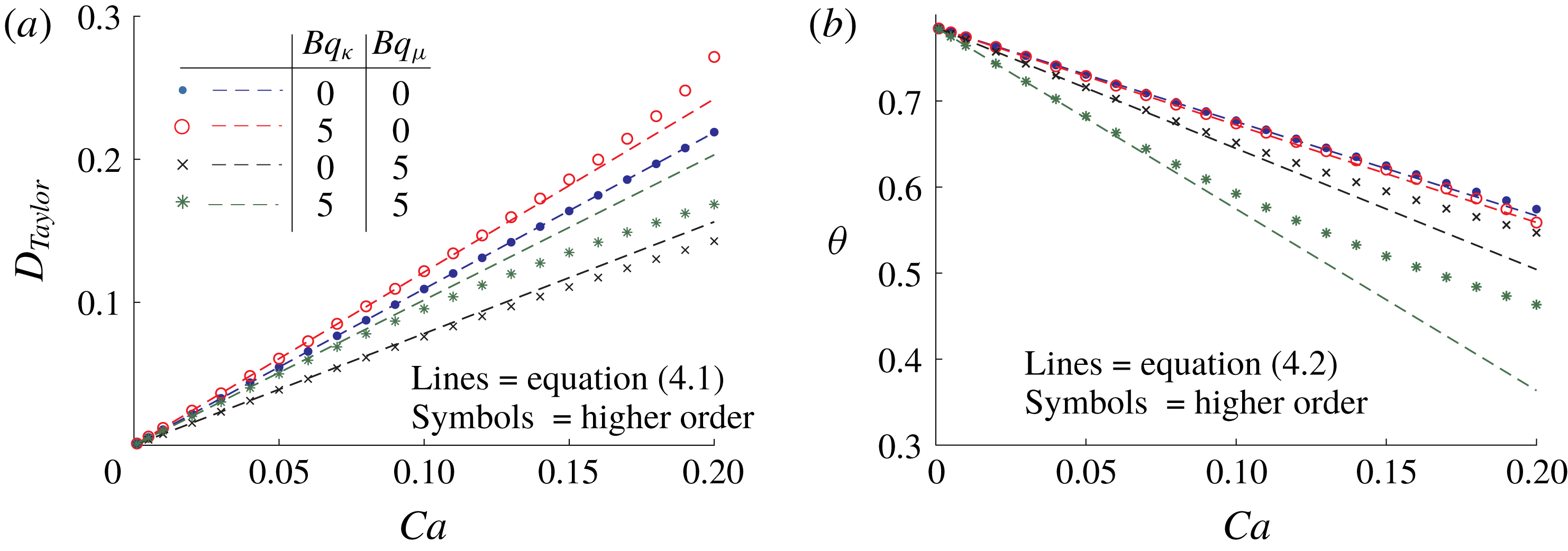
(a) Taylor deformation parameter and (b) inclination angle in steady-state shear flow for
 $Ca\ll 1$
. Lines are leading-order perturbation theories from (4.1) and (4.2). Symbols are higher-order theories from solving the nonlinear equations (3.1)–(3.2) for the steady-state droplet shape tensor
 $\unicode[STIX]{x1D60B}_{ij}$
. The viscosity ratio is
 $\unicode[STIX]{x1D706}=1$
.



In figure 2, we plot the Taylor deformation parameter
 $D_{Taylor}$
and inclination angle
 $\unicode[STIX]{x1D703}_{shear}$
in shear flow, using the lowest-order theories listed here and higher-order theories from solving the nonlinear equations (3.1)–(3.2) for the steady-state droplet shape tensor
 $\unicode[STIX]{x1D60B}_{ij}$
. Overall, we see that the first-order theory compares well with the higher-order theory for
 $Ca<0.1$
. Significant deviations between the two theories occur for
 $Ca>0.1$
when both
 $Bq_{\unicode[STIX]{x1D705}}$
and
 $Bq_{\unicode[STIX]{x1D707}}$
are significantly larger than one (in the case examined,
 $Bq_{\unicode[STIX]{x1D705}}=Bq_{\unicode[STIX]{x1D707}}=5$
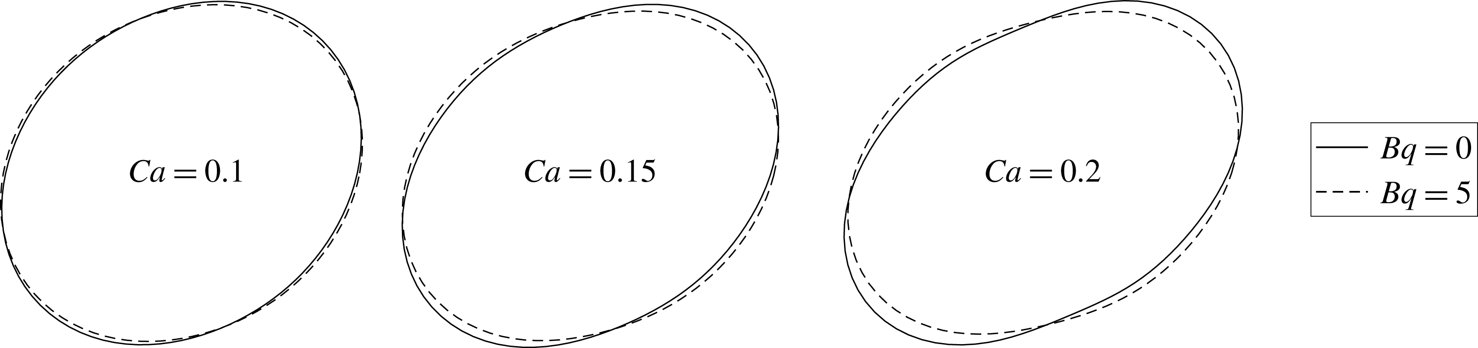
). A picture of the droplet shape as a function of capillary number is shown in figure 3. As mentioned previously, the surface moduli decreases the droplet deformation when
 $Bq_{\unicode[STIX]{x1D707}}=Bq_{\unicode[STIX]{x1D705}}$
. Departures from an ellipsoid only start becoming visually apparent for
 $Ca=0.2$
and above.
4.2 Steady-state droplet shape for
$Ca\sim O(1)$
while
$\unicode[STIX]{x1D706}\gg 1$
or
$Bq_{\unicode[STIX]{x1D705}}\sim Bq_{\unicode[STIX]{x1D707}}\gg 1$


Below are expressions for the Taylor deformation parameter
 $D_{Taylor}$
and the inclination angle
 $\unicode[STIX]{x1D703}_{shear}$
when the droplet has large viscous resistance (
 $\unicode[STIX]{x1D706}\,\gg \,1$
or
 $Bq_{\unicode[STIX]{x1D705}}\,\sim \,Bq_{\unicode[STIX]{x1D707}}\,\gg \,1$
). The results are in terms of the coefficients
 $\hat{a}_{E}$
and
 $\hat{a}_{D}$
in the droplet shape evolution (3.5) and (3.6). These coefficients are listed in (3.10) and (3.11) for the following two cases: (i)
 $\unicode[STIX]{x1D716}=\unicode[STIX]{x1D706}^{-1}\ll 1$
and
 $Bq_{\unicode[STIX]{x1D705}},Bq_{\unicode[STIX]{x1D707}}\sim O(1)$
– i.e. the droplet’s interior viscosity is the dominant resistance, and (ii)
 $\unicode[STIX]{x1D716}=Bq_{\unicode[STIX]{x1D707}}^{-1}\sim Bq_{\unicode[STIX]{x1D705}}^{-1}\ll 1$
and
 $\unicode[STIX]{x1D706}\sim O(1)$
– i.e. the interfacial viscosity is the dominant resistance. The expressions below are expanded to the appropriate power of the small parameter
 $\unicode[STIX]{x1D716}$
 $$\begin{eqnarray}D_{Taylor}={\displaystyle \frac{1}{2}}\hat{a}_{E}(1+\hat{a}_{E})+O(\unicode[STIX]{x1D716}^{3}),\quad \unicode[STIX]{x1D703}_{shear}=-{\displaystyle \frac{1}{2}}{\displaystyle \frac{\hat{a}_{D}}{Ca}}+O(\unicode[STIX]{x1D716}^{2}).\end{eqnarray}$$
When the Boussinesq numbers are large
 $(Bq_{\unicode[STIX]{x1D707}}\sim Bq_{\unicode[STIX]{x1D705}}\gg 1)$
, we find the Taylor deformation parameter decreases when either
 $Bq_{\unicode[STIX]{x1D705}}$
or
 $Bq_{\unicode[STIX]{x1D707}}$
increases. This behaviour is different than the previous subsection, where the dilational surface viscosity increases the droplet deformation. If the surface viscosities are zero, i.e.
 $Bq_{\unicode[STIX]{x1D705}}=Bq_{\unicode[STIX]{x1D707}}=0$
, we obtain the same results for a clean droplet as outlined in Rallison (Reference Rallison1980).
4.3 Interpolating between regimes and new expression for droplet inclination angle
One can develop expressions for droplet shape that interpolate between the regimes listed in the previous two subsections. The results are valid regardless of the small parameter used in the perturbation expansion, as long as the droplet’s shape departs weakly from a sphere. Below is the expression written by Flumerfelt (Reference Flumerfelt1980) for the Taylor deformation
 $D_{Taylor}$
in shear flow. This calculation agrees remarkably well with boundary element simulations (Gounley et al.
Reference Gounley, Boedec, Jaeger and Leonetti2016) over a wide range of capillary numbers, viscosity ratios, and surface moduli.
 $$\begin{eqnarray}D_{Taylor,Flum}={\displaystyle \frac{1}{2}}\unicode[STIX]{x1D6FC}_{0}Ca{\displaystyle \frac{1}{\sqrt{1+(Ca/a_{D,far})^{2}}}};\qquad a_{D,far}=\lim _{\unicode[STIX]{x1D706}\sim Bq_{\unicode[STIX]{x1D705}}\sim Bq_{\unicode[STIX]{x1D707}}\rightarrow \infty }a_{D}.\end{eqnarray}$$
In the above equation,
 $a_{D,far}$
is equal to the coefficient
 $a_{D}$
in shape equation (3.1) in the limit
 $\unicode[STIX]{x1D706}^{-1}\sim Bq_{\unicode[STIX]{x1D705}}^{-1}\sim Bq_{\unicode[STIX]{x1D707}}^{-1}\rightarrow 0$
(see (D 5) in appendix D for full expression). The coefficient
 $\unicode[STIX]{x1D6FC}_{0}$
is the Taylor deformation parameter defined in (4.1), which is equal to
 $\unicode[STIX]{x1D6FC}_{0}=-a_{E}/a_{D}$
. When
 $Ca\ll 1$
, this expression recovers the small-
 $Ca$
expansion in (4.1). When the bulk viscosity is large (
 $\unicode[STIX]{x1D706}\gg 1$
,
 $Bq_{\unicode[STIX]{x1D705}}\sim Bq_{\unicode[STIX]{x1D707}}\sim O(1)$
) or the surface viscosities are large (
 $\unicode[STIX]{x1D706}\sim O(1),Bq_{\unicode[STIX]{x1D707}}\sim Bq_{\unicode[STIX]{x1D705}}\gg 1$
), the expression recovers (4.3) to leading order. When the interfacial viscosities vanish, the above expression is the same as the clean-droplet theory described by Cox (Reference Cox1969).
Flumerfelt (Reference Flumerfelt1980) uses the small-
 $\unicode[STIX]{x1D716}$
droplet evolution equation (3.5) to calculate the inclination angle in the small-deformation regime. In shear flow, the steady-state value is:
 $$\begin{eqnarray}\unicode[STIX]{x1D703}_{shear,Flum}={\displaystyle \frac{\unicode[STIX]{x03C0}}{4}}+{\displaystyle \frac{1}{2}}\tan ^{-1}\left({\displaystyle \frac{Ca}{a_{D,far}}}\right).\end{eqnarray}$$
This expression is the same as the clean-drop result in Cox (Reference Cox1969) when
 $Bq_{\unicode[STIX]{x1D705}}=Bq_{\unicode[STIX]{x1D707}}=0$
. Unfortunately, this theory does not recover the low-
 $Ca$
expansion in (4.2). In fact, this is a well-documented shortcoming of Cox’s theory on clean drops. The above expression fails spectacularly for equiviscous droplets (
 $\unicode[STIX]{x1D706}=1,Bq_{\unicode[STIX]{x1D705}}=Bq_{\unicode[STIX]{x1D707}}=0$
) when the capillary number is beyond
 $Ca>0.01$
.
We propose another expression for the inclination angle that correctly interpolates between the regimes listed in the previous two subsections. In this derivation, we use the small-
 $\unicode[STIX]{x1D716}$
droplet evolution equation in (3.5), but replace the limiting value of coefficients
 $[\hat{a}_{E},\hat{a}_{D},\ldots ]$
with the full values
 $[a_{E},a_{D},\ldots ]$
. The rationale for this operation is that it yields an inclination angle that is valid to
 $O(\unicode[STIX]{x1D716})$
for all regimes of small deformation, i.e.
 $\unicode[STIX]{x1D716}=Ca,Bq_{\unicode[STIX]{x1D707}}^{-1}$
, or
 $\unicode[STIX]{x1D706}^{-1}$
. Solving for the inclination angle in shear flow gives:
 $$\begin{eqnarray}\unicode[STIX]{x1D703}_{shear,interp}={\displaystyle \frac{\unicode[STIX]{x03C0}}{4}}+{\displaystyle \frac{1}{2}}\tan ^{-1}\left({\displaystyle \frac{Ca}{a_{D}}}\right).\end{eqnarray}$$
This is the same result as Flumerfelt but uses the coefficient
 $a_{D}$
instead of the limiting value
 $a_{D,far}=\lim _{\unicode[STIX]{x1D706}\sim Bq_{\unicode[STIX]{x1D707}}\sim Bq_{\unicode[STIX]{x1D705}}\rightarrow \infty }a_{D}$
. As far as we are aware, researchers have not used the above equation to describe droplet inclination angle. We will first compare this expression to numerical simulations of clean droplets, and then examine a droplet with a viscous interface.
4.4 Comparison with boundary element simulations, clean droplets
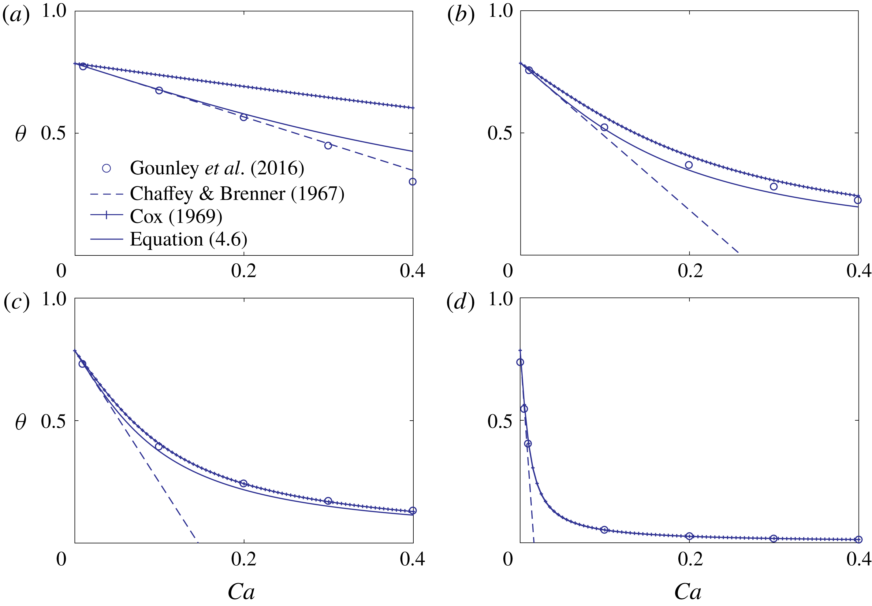
Inclination angle versus capillary number for a clean drop. (a)
 $\unicode[STIX]{x1D706}=1$
, (b)
 $\unicode[STIX]{x1D706}=5$
, (c)
 $\unicode[STIX]{x1D706}=10$
, (d)
 $\unicode[STIX]{x1D706}=100$
. Circles are boundary element simulations from Gounley et al. (Reference Gounley, Boedec, Jaeger and Leonetti2016). Dotted lines correspond to the small-
 $Ca$
theory from Chaffey & Brenner (Reference Chaffey and Brenner1967), which is equivalent to (4.2). The lines with crosses correspond to the small-deformation theory from Cox (Reference Cox1969), which is equivalent to (4.5). The solid lines correspond to our proposed model (4.6), which captures the limits
 $Ca\ll 1$
and
 $\unicode[STIX]{x1D706}\gg 1$
properly.

Figure 4 plots the inclination angle of clean droplets for a wide range of capillary numbers and viscosity ratios. The circles are boundary element simulations from Gounley et al. (Reference Gounley, Boedec, Jaeger and Leonetti2016), while the lines are three theoretical expressions for the inclination angle: (i) small-
 $Ca$
theory, which is captured by (4.2) and is equal to the expressions by Chaffey & Brenner (Reference Chaffey and Brenner1967), (ii) small-deformation theory, which is captured by (4.5) and is equal to Cox (Reference Cox1969), and (iii) the modified expression in (4.6) that correctly interpolates between the regimes
 $Ca\ll 1$
and
 $\unicode[STIX]{x1D706}\gg 1$
. The modified expression (4.6) agrees well with the boundary element simulations over a wide range of viscosity ratios (
 $1<\unicode[STIX]{x1D706}<1000$
) and capillary numbers
 $(Ca<0.3)$
. The
 $Ca\ll 1$
theory from Chaffey & Brenner (Reference Chaffey and Brenner1967) matches simulations well only for viscosity ratio
 $\unicode[STIX]{x1D706}=1$
, while the small-deformation theory from Cox (Reference Cox1969) matches well only for
 $\unicode[STIX]{x1D706}>5$
. In the next subsection, we test our modified theory on droplets with a viscous interface.
4.5 Comparison with boundary element simulations, droplets with a viscous interface
This subsection examines the deformation of a droplet in shear flow when the droplet’s surface has interfacial viscosity. We compare the results from our deformation theories to the boundary element simulations from Gounley et al. (Reference Gounley, Boedec, Jaeger and Leonetti2016).
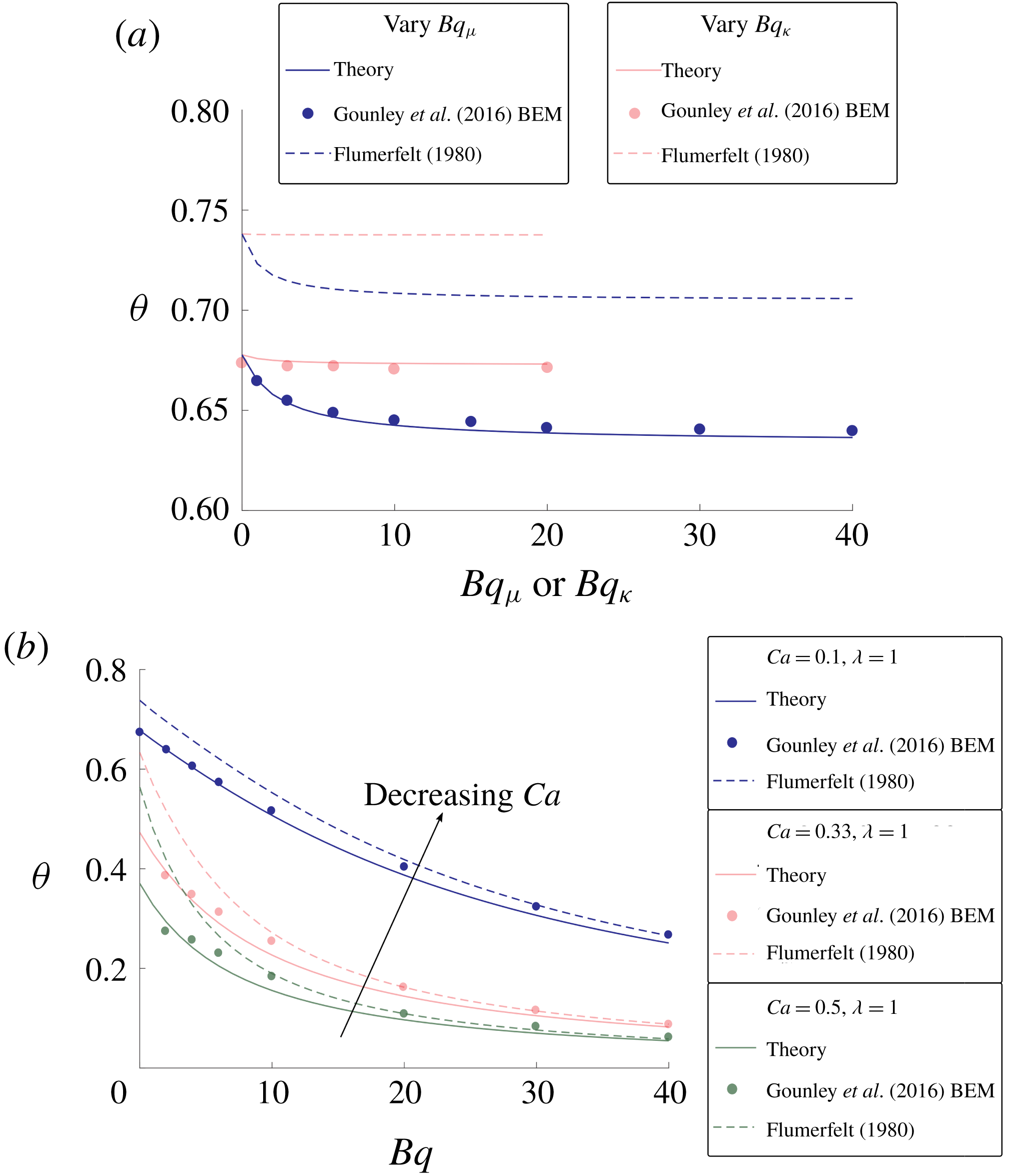
Figure 5(a) plots the inclination angle of droplets in the small-
 $Ca$
regime when
 $Bq_{\unicode[STIX]{x1D705}}$
or
 $Bq_{\unicode[STIX]{x1D707}}\sim O(1)$
. In this regime, previous theories by Flumerfelt (Reference Flumerfelt1980) (e.g. (4.5)) grossly miscalculate the inclination angle, while the expressions developed by us (4.6) agree quantitatively with simulations. Figure 5(b) plots the inclination angle when the droplet has large surface viscosity (
 $Bq_{\unicode[STIX]{x1D705}}=Bq_{\unicode[STIX]{x1D707}}=Bq\gg 1$
). Flumerfelt’s theory (4.5) was derived with this condition in mind, and hence it is no surprise that it agrees well with the simulations. However, there appears to be significant discrepancies when
 $Bq=Bq_{\unicode[STIX]{x1D705}}=Bq_{\unicode[STIX]{x1D707}}\sim O(1)$
and below. The current theory (4.6) appears to do a better job matching the simulations over the entire range of Boussinesq numbers studied.
Inclination angle versus Boussinesq number. We compare our leading-order theory that interpolates between small-deformation regimes (4.6) to boundary element simulations (Gounley et al.
Reference Gounley, Boedec, Jaeger and Leonetti2016) and older droplet deformation theories ((4.5), which is equivalent to Flumerfelt (Reference Flumerfelt1980)). (a) The blue curves vary
 $Bq_{\unicode[STIX]{x1D707}}$
while keeping
 $Bq_{\unicode[STIX]{x1D705}}=0$
. The red curves vary
 $Bq_{\unicode[STIX]{x1D705}}$
while keeping
 $Bq_{\unicode[STIX]{x1D707}}=0$
. The capillary number and viscosity ratio are
 $Ca=0.1$
and
 $\unicode[STIX]{x1D706}=1$
. (b) Vary
 $Bq=Bq_{\unicode[STIX]{x1D705}}=Bq_{\unicode[STIX]{x1D707}}$
. Here,
 $\unicode[STIX]{x1D706}=1$
and
 $Ca=0.1,$
 $0.33$
and
 $0.5$
.

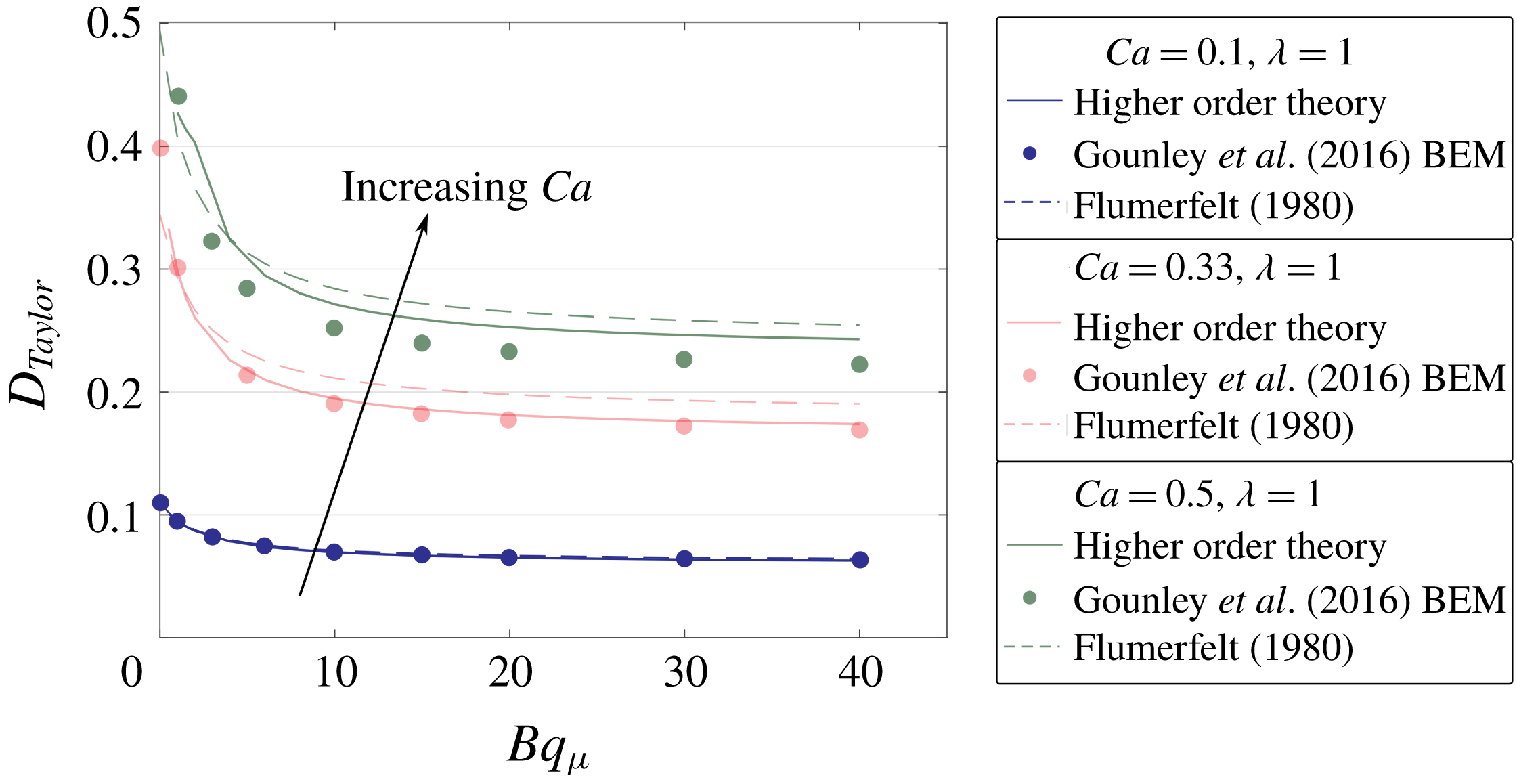
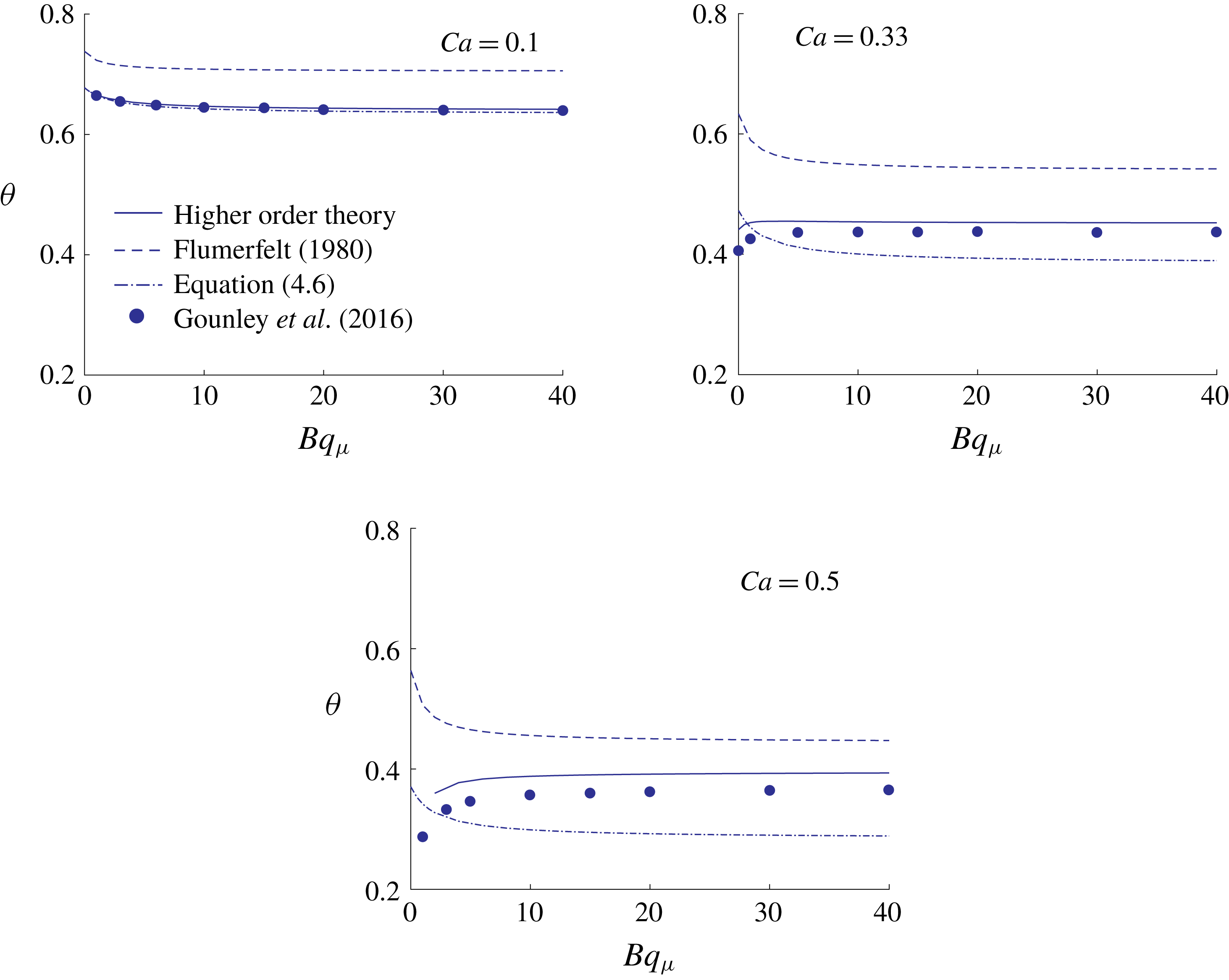
If the droplet deformation is no longer small, one will not expect the leading-order theories (i.e. (4.4) and (4.6)) to capture the Taylor deformation parameter and inclination angle quantitatively. Figures 6 and 7 demonstrate such an example. These figures examine the effect of shear surface viscosity on droplet shape for capillary numbers
 $Ca=0.1$
,
 $0.33$
and
 $0.5$
. The leading-order theories developed by us (i.e. (4.4) and (4.6)) quantitatively match the simulations at low capillary number (
 $Ca=0.1$
), but do a poor job at
 $Ca=0.33$
and
 $Ca=0.5$
, where the deformation is no longer weak. For the latter two cases, one can obtain better agreement with the simulations if one uses higher-order theories – i.e. one solves the nonlinear equations (3.1)–(3.2) for the steady-state droplet shape tensor
 $\unicode[STIX]{x1D60B}_{ij}$
. We obtain nearly quantitative agreement at
 $Ca=0.33$
, while getting reasonable agreement at
 $Ca=0.5$
.
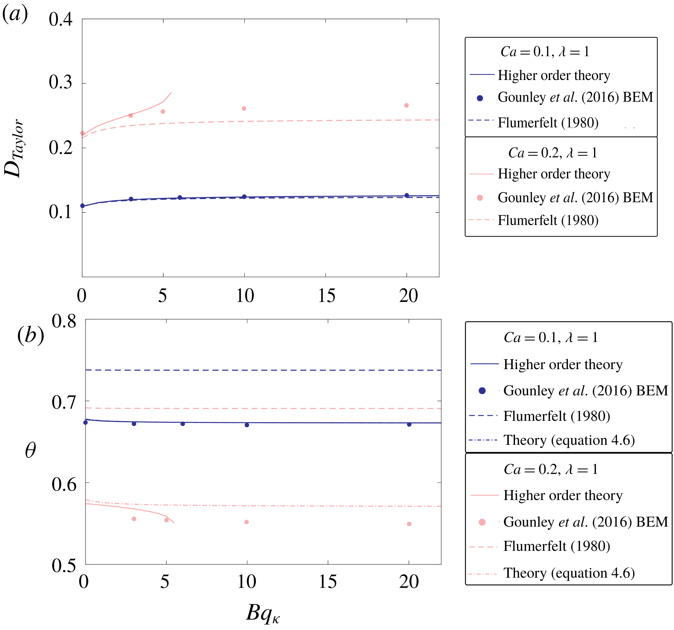
Unfortunately, the higher-order theory does not perform as well when one examines the effect of dilational viscosity only (figure 8). At low capillary numbers (
 $Ca=0.1$
), both leading-order and higher-order theories match the boundary element simulations, but the higher-order theory starts deviating from the simulations when
 $Ca\geqslant 0.2$
. In figure 8, we terminate the curves for the higher-order theory when the calculated droplet shape becomes unphysical or unsteady. We are unable to reproduce physically relevant shapes beyond a critical dilational Boussinesq number
 $Bq_{\unicode[STIX]{x1D705}}$
, probably due to the fact that we need higher-order terms in the perturbation expansion to describe the droplet shape equations (3.1) and (3.2) accurately. It will be interesting to see if one can obtain better agreement if one calculates the
 $O(Ca)$
contribution to the shape tensor
 $\unicode[STIX]{x1D60B}_{ijmn}$
as well as 6th-order harmonic contributions (i.e. a fully consistent,
 $O(Ca^{3})$
theory for the droplet radius).
Effect of
 $Bq_{\unicode[STIX]{x1D707}}$
on Taylor deformation parameter. Solid lines are higher-order theories obtained by solving the nonlinear equations (3.1) and (3.2) for the steady-state droplet shape tensor
 $\unicode[STIX]{x1D60B}_{ij}$
. The dotted lines are older theories for Taylor deformation parameter (Flumerfelt (Reference Flumerfelt1980), i.e. (4.4)). Symbols are boundary element simulations from Gounley et al. (Reference Gounley, Boedec, Jaeger and Leonetti2016). The viscosity ratio is
 $\unicode[STIX]{x1D706}=1$
and the dilational viscosity is zero (
 $Bq_{\unicode[STIX]{x1D705}}=0$
).

Effect of
 $Bq_{\unicode[STIX]{x1D707}}$
on droplet inclination angle in shear flow. Symbols are boundary element simulations from Gounley et al. (Reference Gounley, Boedec, Jaeger and Leonetti2016). Dashed lines correspond to the older theory from Flumerfelt (Reference Flumerfelt1980) (i.e. (4.5)). Dash-dotted lines correspond to the modified theory from (4.6). Solid lines are higher-order theories obtained by solving the nonlinear equations (3.1) and (3.2) for the steady-state droplet shape tensor
 $\unicode[STIX]{x1D60B}_{ij}$
. The viscosity ratio is
 $\unicode[STIX]{x1D706}=1$
and the dilational viscosity is zero (
 $Bq_{\unicode[STIX]{x1D705}}=0$
).

Effect of
 $Bq_{\unicode[STIX]{x1D705}}$
on (a) Taylor deformation parameter and (b) inclination angle in shear flow. In (a), solid lines are higher-order theories obtained by solving the nonlinear equations (3.1) and (3.2) for the steady-state droplet shape tensor
 $\unicode[STIX]{x1D60B}_{ij}$
. The dotted lines are older theories for Taylor deformation parameter (Flumerfelt (Reference Flumerfelt1980)). Symbols are boundary element simulations from Gounley et al. (Reference Gounley, Boedec, Jaeger and Leonetti2016). We use the same convention in (b), with an additional dash-dotted line that represents the modified theory for droplet inclination angle in (4.6). The viscosity ratio is
 $\unicode[STIX]{x1D706}=1$
and the shear surface viscosity is zero (
 $Bq_{\unicode[STIX]{x1D707}}=0$
).

4.6 Time-dependent deformation
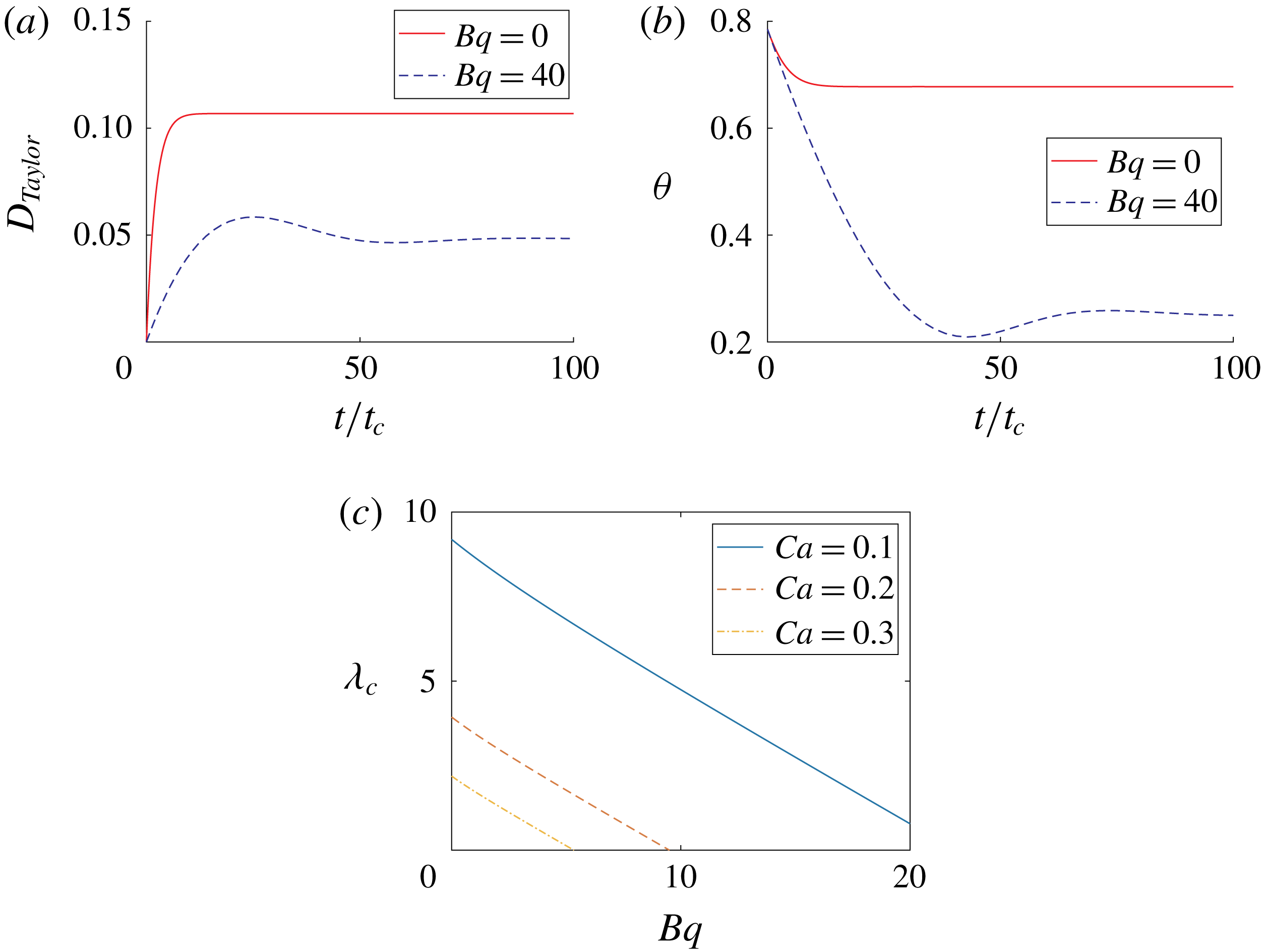
In this section, we describe the time-dependent dynamics of a droplet as it reaches its steady-state deformation. Typically, one observes two different behaviours: (i) the droplet reaches its steady shape in a seemingly monotonic fashion, or (ii) the drop undershoots and overshoots its steady deformation like a damped, harmonic oscillator (cf. figure 9
a,b for examples). The latter behaviour occurs when the viscous resistance of the droplet is significant (for a clean drop, it appears to occur when
 $\unicode[STIX]{x1D706}\geqslant 4$
for
 $Ca\approx 0.25$
, see Torza, Cox & Mason (Reference Torza, Cox and Mason1972) for details). We note that Erni, Fischer & Windhab (Reference Erni, Fischer and Windhab2005) observe this damped behaviour for droplets with a viscoelastic surface.
To develop a leading-order theory that describes these motions, we will take droplet evolution equation (3.5), replace coefficients
 $[\hat{a}_{E},\hat{a}_{D},\ldots ]$
with
 $[a_{E},a_{D},\ldots ]$
, and drop the terms that are quadratic in
 $\unicode[STIX]{x1D60B}_{ij}$
and contain
 $\unicode[STIX]{x1D60B}_{ik}\unicode[STIX]{x1D60C}_{kj}$
. These operations yield an evolution equation that correctly calculates the Taylor deformation parameter and inclination angle to
 $O(\unicode[STIX]{x1D716})$
for all regions of small deformation – i.e.
 $\unicode[STIX]{x1D716}=Ca,Bq_{\unicode[STIX]{x1D707}}^{-1}$
, or
 $\unicode[STIX]{x1D706}^{-1}$
. To be explicit, we write the evolution equation below:
 $$\begin{eqnarray}{\displaystyle \frac{\unicode[STIX]{x2202}\unicode[STIX]{x1D60B}_{ij}}{\unicode[STIX]{x2202}t_{H}}}+2Sd_{2}[\unicode[STIX]{x1D60B}_{ik}\unicode[STIX]{x1D6FA}_{kj}]={\displaystyle \frac{a_{E}}{\unicode[STIX]{x1D716}}}\unicode[STIX]{x1D60C}_{ij}+{\displaystyle \frac{a_{D}}{Ca}}\unicode[STIX]{x1D60B}_{ij}.\end{eqnarray}$$
In the above equation,
 $t_{H}=\dot{\unicode[STIX]{x1D6FE}}\tilde{t}$
is a non-dimensional time that is represents the total accumulated strain on the droplet. Expressions for coefficients
 $a_{E}$
and
 $a_{D}$
are listed in (D 3) and (D 4) in appendix D.
Time-dependent motion of droplet in shear flow. For (a) and (b), we solve the leading-order, time-dependent equations (4.7) for the shape tensor
 $\unicode[STIX]{x1D60B}_{ij}$
and plot the Taylor deformation parameter and inclination angle, respectively. The plots examine
 $Ca=0.1$
and
 $\unicode[STIX]{x1D706}=1$
for different values of
 $Bq=Bq_{\unicode[STIX]{x1D705}}=Bq_{\unicode[STIX]{x1D707}}$
. We observe two distinct types of dynamics: the droplet transitions to its steady state in a seemingly monotonic fashion, or it approaches steady state via damped oscillations. The time is normalized by the capillary time scale
 $t_{c}=\unicode[STIX]{x1D702}R/\unicode[STIX]{x1D70E}$
. (c) Critical viscosity ratio at which the decay time scale and oscillatory time scale are equal, i.e.
 $|a_{D}|=Ca$
.

In shear flow (
 $u_{1}^{\infty }=x_{2}$
,
 $u_{2}^{\infty }=u_{3}^{\infty }=0$
), the only non-zero components of the deformation tensor are
 $\unicode[STIX]{x1D60B}_{11}$
,
 $\unicode[STIX]{x1D60B}_{22}$
and
 $\unicode[STIX]{x1D60B}_{12}$
. Solving the set of linear ODEs for these components gives the following growth rates:
 $\unicode[STIX]{x1D60B}_{jk}\sim \exp (st)$
, where
 $s=\{a_{D}/Ca,a_{D}/Ca+\text{i},a_{D}/Ca-\text{i}\}$
, where
 $\text{i}=\sqrt{-1}$
is an imaginary number. The coefficient
 $a_{D}<0$
, so the linear theory always predicts a decay via damped oscillations to steady-state values. In dimensional terms, the time scale of the decay is
 $\tilde{t}_{decay}=t_{c}/|a_{D}|=\unicode[STIX]{x1D702}R/(|a_{D}|\unicode[STIX]{x1D70E})$
, i.e. the capillary time scale divided by
 $|a_{D}|$
. The time scale of the oscillations is
 $\tilde{t}_{oscill}=\dot{\unicode[STIX]{x1D6FE}}^{-1}$
, i.e. the flow time scale. In practice, one cannot experimentally observe oscillations if
 $\tilde{t}_{oscill}\gg \tilde{t}_{decay}$
, in other words
 $|a_{D}|\gg Ca$
. The oscillations become visually apparent only when
 $|a_{D}|\sim Ca$
. This latter condition allows one to develop scaling relationships to determine when the drop transitions between the regimes of damped oscillations versus exponential approach to steady state. For example, when
 $\unicode[STIX]{x1D706}\gg 1$
,
 $|a_{D}|\sim \unicode[STIX]{x1D706}^{-1}$
, and hence the critical capillary number that demarcates the two regimes scales as
 $Ca_{c}\sim \unicode[STIX]{x1D706}^{-1}$
. Similarly, when
 $Bq_{\unicode[STIX]{x1D705}}=Bq_{\unicode[STIX]{x1D707}}=Bq\gg 1$
, the critical capillary number
 $Ca_{c}\sim Bq^{-1}$
. In fact, Gounley et al. (Reference Gounley, Boedec, Jaeger and Leonetti2016) observe the latter relationship empirically through their boundary element simulations, although no explanation was provided for why this scaling exists.
To get a rough estimate for when one observes visual oscillations, we plot the critical viscosity ratio
 $\unicode[STIX]{x1D706}_{c}$
under which the two time scales match, i.e.
 $|a_{D}|=Ca$
for various values of capillary number
 $Ca$
and Boussinesq numbers
 $Bq=Bq_{\unicode[STIX]{x1D707}}=Bq_{\unicode[STIX]{x1D705}}$
(figure 9
c). The exact transition will be somewhere around this viscosity ratio, but cannot be exactly predicted from leading-order theory. Only trends can be observed. We see that larger surface viscosities leads to a smaller critical viscosity ratio. For sufficiently large Boussinesq numbers, the droplet’s deformation will always experience damped oscillation. Although not mentioned here, the effect of higher-order terms in the shape evolution equations is to dampen the oscillations slightly.
5 Results, droplet rheology and breakup
In this section, we discuss the steady-state rheology of a dilute suspension of droplets. We examine theories that solve the particle stresslet to
 $O(Ca)$
and
 $O(Ca^{2})$
through regular perturbation expansions. We denote the
 $O(Ca)$
expansion as the leading-order theory, and the
 $O(Ca^{2})$
expansion as the higher-order theory. The leading-order theory gives the normal stress differences created by droplet deformation, while the higher-order theory gives additional information such as shear thinning and breakup. The summary of the main findings are below.
5.1 Leading-order theory,
$Ca\ll 1$
while
$\unicode[STIX]{x1D706},Bq_{\unicode[STIX]{x1D705}},Bq_{\unicode[STIX]{x1D707}}\sim O(1)$


The leading-order theory predicts the steady-state, extra stress in the suspension to be:
 $$\begin{eqnarray}\displaystyle \unicode[STIX]{x1D70F}_{ij}^{extra} & = & \displaystyle \unicode[STIX]{x1D719}\unicode[STIX]{x1D60C}_{ij}{\displaystyle \frac{5\unicode[STIX]{x1D706}^{\ast }+2}{\unicode[STIX]{x1D706}^{\ast }+1}}-\unicode[STIX]{x1D719}Ca{\displaystyle \frac{16}{5}}\unicode[STIX]{x1D6FC}_{0}^{2}Sd_{2}[\unicode[STIX]{x1D60C}_{ik}\unicode[STIX]{x1D6FA}_{kj}]\nonumber\\ \displaystyle & & \displaystyle +\,\unicode[STIX]{x1D719}Ca\left[{\displaystyle \frac{6\unicode[STIX]{x1D6FC}_{0}}{35}}{\displaystyle \frac{25\unicode[STIX]{x1D706}^{\ast 2}+41\unicode[STIX]{x1D706}+24Bq_{\unicode[STIX]{x1D705}}+4}{(\unicode[STIX]{x1D706}^{\ast }+1)^{2}}}Sd_{2}[\unicode[STIX]{x1D60C}_{ik}\unicode[STIX]{x1D60C}_{kj}]\right].\end{eqnarray}$$
In the above expression,
 $\unicode[STIX]{x1D706}^{\ast }=\unicode[STIX]{x1D706}+6/5\times Bq_{\unicode[STIX]{x1D705}}+4/5\times Bq_{\unicode[STIX]{x1D707}}$
is an effective viscosity ratio, and
 $\unicode[STIX]{x1D6FC}_{0}$
is the steady-state deformation of the droplet given in (4.1). The first term is Einstein viscosity of a dilute emulsion. We see that the emulsion behaves as an emulsion of clean droplets with an effective interior viscosity
 $\unicode[STIX]{x1D706}^{\ast }\unicode[STIX]{x1D702}$
. This result was originally discovered by Oldroyd (Reference Oldroyd1955) and replicated in many other papers (Danov Reference Danov2001). As far as we are aware, the
 $O(\unicode[STIX]{x1D719}Ca)$
stress has not been reported. This is the second-order fluid correction, and it depends quadratically on the symmetric, traceless product of the rate-of-strain tensor
 $\unicode[STIX]{x1D60C}_{ij}$
with itself, as well as the symmetric, traceless product of
 $\unicode[STIX]{x1D60C}_{ij}$
with the vorticity tensor
 $\unicode[STIX]{x1D6FA}_{ij}$
. When
 $Bq_{\unicode[STIX]{x1D707}}$
and
 $Bq_{\unicode[STIX]{x1D705}}$
are zero, we recover the same expression as Schowalter, Chaffey & Brenner (Reference Schowalter, Chaffey and Brenner1968) and Vlahovska et al. (Reference Vlahovska, Bławzdziewicz and Loewenberg2009a
) for a clean interface. Below are limiting expressions for shear flow and uniaxial extensional flow. Please refer to § 2.4 for definitions of the non-dimensional extra-shear viscosity
 $[\unicode[STIX]{x1D702}]$
, normal stress coefficients
 $\unicode[STIX]{x1D713}_{1}$
and
 $\unicode[STIX]{x1D713}_{2}$
, and Trouton ratio
 $[Tr]$
.
Shear rheology: In shear flow, (i.e.
 $u_{1}^{\infty }=x_{2}$
,
 $u_{2}^{\infty }=u_{3}^{\infty }=0$
), we find the extra-shear viscosity and normal stress coefficients to be:
 $$\begin{eqnarray}\displaystyle & \displaystyle [\unicode[STIX]{x1D702}]={\displaystyle \frac{5\unicode[STIX]{x1D706}^{\ast }+2}{2\unicode[STIX]{x1D706}^{\ast }+2}}, & \displaystyle\end{eqnarray}$$
 $$\begin{eqnarray}\displaystyle & \displaystyle \unicode[STIX]{x1D713}_{1}={\textstyle \frac{8}{5}}\unicode[STIX]{x1D6FC}_{0}^{2}, & \displaystyle\end{eqnarray}$$
 $$\begin{eqnarray}\displaystyle & \displaystyle \unicode[STIX]{x1D713}_{2}={\displaystyle \frac{3\unicode[STIX]{x1D6FC}_{0}}{70}}{\displaystyle \frac{1}{(\unicode[STIX]{x1D706}^{\ast }+1)^{2}}}(25\unicode[STIX]{x1D706}^{\ast 2}+41\unicode[STIX]{x1D706}+24Bq_{\unicode[STIX]{x1D705}}+4)-{\displaystyle \frac{4}{5}}\unicode[STIX]{x1D6FC}_{0}^{2}. & \displaystyle\end{eqnarray}$$
In the above expressions,
 $\unicode[STIX]{x1D6FC}_{0}$
is a steady-state deformation parameter and
 $\unicode[STIX]{x1D706}^{\ast }$
is an effective viscosity ratio, both of which are defined in (4.1). At this level of approximation, the normal stress coefficients (5.3) and (5.4) are independent of shear rate (a.k.a., capillary number), but depend on the viscosity ratio
 $\unicode[STIX]{x1D706}$
and the Boussinesq numbers
 $Bq_{\unicode[STIX]{x1D705}}$
and
 $Bq_{\unicode[STIX]{x1D707}}$
. We find that the first normal stress coefficient
 $\unicode[STIX]{x1D713}_{1}$
is positive and the second normal stress coefficient
 $\unicode[STIX]{x1D713}_{2}$
is negative, with
 $|\unicode[STIX]{x1D713}_{1}|>|\unicode[STIX]{x1D713}_{2}|$
. In figures 10 and 11, we examine how
 $\unicode[STIX]{x1D713}_{1}$
and
 $\unicode[STIX]{x1D713}_{2}$
vary with the Boussinesq numbers
 $Bq_{\unicode[STIX]{x1D705}}$
and
 $Bq_{\unicode[STIX]{x1D707}}$
. We note that
 $\unicode[STIX]{x1D713}_{1}$
is proportional to the square of the Taylor deformation parameter
 $D_{Taylor}=\unicode[STIX]{x1D6FC}_{0}/2$
, and thus follows the same trends as
 $D_{Taylor}$
. In particular, if one increases both Boussinesq numbers while keeping the ratio
 $\unicode[STIX]{x1D6FD}=Bq_{\unicode[STIX]{x1D705}}/Bq_{\unicode[STIX]{x1D707}}$
constant, we find that both drop deformation and
 $\unicode[STIX]{x1D713}_{1}$
increase when
 $\unicode[STIX]{x1D6FD}>2$
(i.e. when surface dilational resistance dominates) and decrease when
 $\unicode[STIX]{x1D6FD}<2$
(i.e. when surface shear resistance becomes more important).
First normal stress coefficient
 $\unicode[STIX]{x1D713}_{1}=(\unicode[STIX]{x1D70F}_{11}-\unicode[STIX]{x1D70F}_{22})/(\unicode[STIX]{x1D719}Ca)$
in shear flow at steady state, using the lowest-order perturbation theories in (5.3). (a) Examine
 $Bq_{\unicode[STIX]{x1D705}}\geqslant Bq_{\unicode[STIX]{x1D707}}$
. (b) Examine
 $Bq_{\unicode[STIX]{x1D707}}\geqslant Bq_{\unicode[STIX]{x1D705}}$
. The viscosity ratio is
 $\unicode[STIX]{x1D706}=1$
for the graphs.

Second normal stress coefficient
 $\unicode[STIX]{x1D713}_{2}=(\unicode[STIX]{x1D70F}_{22}-\unicode[STIX]{x1D70F}_{33})/(\unicode[STIX]{x1D719}Ca)$
in shear flow at steady state, using the lowest-order perturbation theories in (5.4). (a) Examine
 $Bq_{\unicode[STIX]{x1D705}}\geqslant Bq_{\unicode[STIX]{x1D707}}$
. (b) Examine
 $Bq_{\unicode[STIX]{x1D707}}\geqslant Bq_{\unicode[STIX]{x1D705}}$
. The viscosity ratio is
 $\unicode[STIX]{x1D706}=1$
for the graphs.

For the most part, it appears that surface viscosity decreases the magnitude of the second normal stress coefficient
 $|\unicode[STIX]{x1D713}_{2}|$
(figure 11). The one exception we observe appears in figure 11(a) when
 $Bq_{\unicode[STIX]{x1D705}}\sim O(1)$
and the dilational resistance dominates shear resistance (
 $Bq_{\unicode[STIX]{x1D707}}/Bq_{\unicode[STIX]{x1D705}}\leqslant 0.25$
). In this region, the second normal stress coefficient has a non-monotonic dependence on the surface dilational viscosity.
We note that a droplet in wall-bound shear flow experiences a lift away from the wall due to the reflection of its force dipole (Smart & Leighton Jr Reference Smart and Leighton1991). The droplet’s lift velocity is proportional to
 $\unicode[STIX]{x1D713}_{1}-\unicode[STIX]{x1D713}_{2}$
(see (2.17)), hence we plot
 $\unicode[STIX]{x1D713}_{1}-\unicode[STIX]{x1D713}_{2}$
for different Boussinesq numbers in figure 12. Because the first normal stress coefficient
 $\unicode[STIX]{x1D713}_{1}$
is typically larger in magnitude than the second normal stress coefficient
 $\unicode[STIX]{x1D713}_{2}$
, the trends one observes for
 $\unicode[STIX]{x1D713}_{1}$
tend to hold for the lift velocity. In other words, the lift tends to increase with increasing
 $Bq_{\unicode[STIX]{x1D705}}$
, but decrease with increasing
 $Bq_{\unicode[STIX]{x1D707}}$
. If both
 $Bq_{\unicode[STIX]{x1D705}}$
and
 $Bq_{\unicode[STIX]{x1D707}}$
change equally, the lift velocity tends to decrease with increasing
 $Bq=Bq_{\unicode[STIX]{x1D705}}=Bq_{\unicode[STIX]{x1D707}}$
. Since
 $\unicode[STIX]{x1D713}_{1}-\unicode[STIX]{x1D713}_{2}$
is always greater than zero, the droplet always migrates away from the wall. We note that for the case when
 $Bq_{\unicode[STIX]{x1D707}}=0$
, the presence of surface dilational viscosity increases the lift velocity above that of a clean droplet.
Difference in normal stress coefficients
 $\unicode[STIX]{x1D713}_{1}-\unicode[STIX]{x1D713}_{2}$
for three cases: (a) vary
 $Bq_{\unicode[STIX]{x1D705}}$
while keeping
 $Bq_{\unicode[STIX]{x1D707}}=0$
, (b) vary
 $Bq=Bq_{\unicode[STIX]{x1D707}}=Bq_{\unicode[STIX]{x1D705}}$
, and (c) vary
 $Bq_{\unicode[STIX]{x1D707}}$
while keeping
 $Bq_{\unicode[STIX]{x1D705}}=0$
. The viscosity ratio is
 $\unicode[STIX]{x1D706}=1$
.

Extensional rheology: For uniaxial extensional flow (i.e.
 $u_{1}^{\infty }=-0.5~x_{1}$
,
 $u_{2}^{\infty }=-0.5~x_{2},u_{3}^{\infty }=x_{3}$
), we write the expression for the excess Trouton ratio:
 $$\begin{eqnarray}\displaystyle [Tr] & = & \displaystyle {\displaystyle \frac{3}{2}}{\displaystyle \frac{5\unicode[STIX]{x1D706}^{\ast }+2}{\unicode[STIX]{x1D706}^{\ast }+1}}+{\displaystyle \frac{9}{70}}\unicode[STIX]{x1D6FC}_{0}Ca{\displaystyle \frac{25\unicode[STIX]{x1D706}^{\ast 2}+41\unicode[STIX]{x1D706}+24Bq_{\unicode[STIX]{x1D705}}+4}{(\unicode[STIX]{x1D706}^{\ast }+1)^{2}}}\nonumber\\ \displaystyle & = & \displaystyle 3[\unicode[STIX]{x1D702}]|_{shear}+\frac{3}{2}Ca\left(\frac{1}{2}\unicode[STIX]{x1D713}_{1}|_{shear}+\unicode[STIX]{x1D713}_{2}|_{shear}\right).\end{eqnarray}$$
Here,
 $\unicode[STIX]{x1D713}_{1}$
and
 $\unicode[STIX]{x1D713}_{2}$
are the normal stress coefficients in shear flow, given by (5.3)–(5.4). We observe that
 $\unicode[STIX]{x1D713}_{1}/2+\unicode[STIX]{x1D713}_{2}$
is greater than zero, which indicates that the Trouton ratio thickens with increasing extension rate (i.e. capillary number). It appears that the dilational surface viscosity plays a more important role in thickening than the shear surface viscosity, since
 $\unicode[STIX]{x1D713}_{1}/2+\unicode[STIX]{x1D713}_{2}$
increases with increasing
 $Bq_{\unicode[STIX]{x1D705}}$
, whereas
 $\unicode[STIX]{x1D713}_{1}/2+\unicode[STIX]{x1D713}_{2}$
decreases with increasing
 $Bq_{\unicode[STIX]{x1D707}}$
. This makes intuitive sense, as one would expect dilational modes to provide the dominant resistance in uniaxial flow.
5.2 Higher-order theory,
$Ca\ll 1$
while
$\unicode[STIX]{x1D706},Bq_{\unicode[STIX]{x1D705}},Bq_{\unicode[STIX]{x1D707}}\sim O(1)$


Extra-shear viscosity of clean drops. Symbols correspond to the
 $O(Ca^{2})$
theory from this manuscript, while the lines correspond to the theories from Vlahovska et al. (Reference Vlahovska, Bławzdziewicz and Loewenberg2009a
). We observe quantitative agreement between the two theories.

Effect of interfacial viscosity on shear thinning. (a) Extra-shear viscosity versus capillary number. Dotted lines are leading-order theory (5.1) and symbols are the
 $O(Ca^{2})$
theory. The extra viscosity in the
 $O(Ca^{2})$
theory takes the form
 $[\unicode[STIX]{x1D702}]=[\unicode[STIX]{x1D702}]_{0}-\unicode[STIX]{x1D701}Ca^{2}$
, where
 $[\unicode[STIX]{x1D702}]_{0}$
is the zero-shear viscosity and
 $\unicode[STIX]{x1D701}$
is the shear thinning coefficient. In (b) and (c), we examine how the shear thinning coefficient
 $\unicode[STIX]{x1D701}$
varies with the dilational and shear Boussinesq numbers
 $Bq_{\unicode[STIX]{x1D705}}$
and
 $Bq_{\unicode[STIX]{x1D707}}$
. For all graphs, the viscosity ratio
 $\unicode[STIX]{x1D706}=1$
.

In this subsection, we numerically compute the droplet extra stress to
 $O(Ca^{2})$
. In particular, we discuss shear thinning, extensional thickening and extensional breakup in the droplet suspension.
Shear flow: In shear flow, the normal stresses are unaltered at
 $O(Ca^{2})$
. Thus, the analytical expressions for the normal stress coefficients remain the same as in (5.3) and (5.4). The primary effect of the
 $O(Ca^{2})$
extra stress is to introduce shear thinning into the suspension. Before we discuss the effect of interfacial viscosity on this phenomenon, we first compare the clean-droplet theories in this manuscript to published results in Vlahovska et al. (Reference Vlahovska, Bławzdziewicz and Loewenberg2009a
).
Figure 13 displays the extra-shear viscosity as a function of capillary number for a suspension of clean droplets (i.e.
 $Bq_{\unicode[STIX]{x1D705}}=Bq_{\unicode[STIX]{x1D707}}=0$
). The symbols are numerical results from our current theories to
 $O(Ca^{2})$
, while the solid lines are
 $O(Ca^{2})$
analytical expressions by Vlahovska et al. (Reference Vlahovska, Bławzdziewicz and Loewenberg2009a
). We see that our theories quantitatively match the known expressions for clean droplets. We thus proceed to examine the effect of surface viscosities on the suspension behaviour.
Figure 14(a) examines how interfacial viscosity alters the shear rheology of droplet suspensions, with the dotted lines representing the
 $O(Ca)$
theory (5.2) and the symbols representing the
 $O(Ca^{2})$
theory. We observe modest shear thinning, with the effect becoming more pronounced beyond
 $Ca>0.1$
. To better visualize the extent of shear thinning, we note that the extra-shear viscosity takes the form
 $$\begin{eqnarray}[\unicode[STIX]{x1D702}]=[\unicode[STIX]{x1D702}]_{0}-\unicode[STIX]{x1D701}\,Ca^{2},\end{eqnarray}$$
where
 $[\unicode[STIX]{x1D702}]_{0}$
is the zero-shear viscosity from the leading-order theory, and
 $\unicode[STIX]{x1D701}$
is the coefficient of shear thinning from the
 $O(Ca^{2})$
theory. A larger value of coefficient
 $\unicode[STIX]{x1D701}$
indicates a greater extent of shear thinning. In figure 14(b,c), we plot the coefficient of shear thinning for various values of Boussinesq numbers
 $Bq_{\unicode[STIX]{x1D707}}$
and
 $Bq_{\unicode[STIX]{x1D705}}$
. For the most part, interfacial viscosity enhances shear thinning compared to a clean droplet. The rationale for this behaviour arises from the ability of droplets to align and stretch along the flow direction. When the dilational Boussinesq number is larger than the shear Boussinesq number (i.e.
 $Bq_{\unicode[STIX]{x1D705}}>Bq_{\unicode[STIX]{x1D707}}$
), the droplet deformation increases compared to a clean droplet and the orientation angle aligns closer to the flow axis (see figure 2). Both of these effects improve shear thinning. Only when
 $Bq_{\unicode[STIX]{x1D707}}\gg Bq_{\unicode[STIX]{x1D705}}$
do we observe anomalous behaviour. In this case, the droplet deformation is reduced compared to a clean droplet, while the orientation angle aligns closer to the flow axis (see figure 2). These effects compete against each other in determining shear thinning behaviour, which leads to a non-monotonic dependence of the shear thinning coefficient with the Boussinesq number
 $Bq_{\unicode[STIX]{x1D707}}$
.
Extensional flow and droplet breakup: figure 15 plots the excess Trouton ratio as a function of capillary number. The dotted line is the
 $O(Ca)$
theory (5.5), and the symbols are the
 $O(Ca^{2})$
theory. In the limit of zero extension rate (i.e.
 $Ca\rightarrow 0$
), the effect of surface viscosity is to increase the extensional viscosity of the solution. The Trouton ratio in this limit is
 $[Tr]\rightarrow 3/2\times (5\unicode[STIX]{x1D706}^{\ast }+2)/(\unicode[STIX]{x1D706}^{\ast }+1)$
, where
 $\unicode[STIX]{x1D706}^{\ast }=\unicode[STIX]{x1D706}+6/5\times Bq_{\unicode[STIX]{x1D705}}+4/5\times Bq_{\unicode[STIX]{x1D707}}$
is an effective viscosity ratio. When the capillary number is beyond zero, the solution thickens – i.e. the Trouton ratio
 $[Tr]$
increases with increasing extension rate. Overall, the
 $O(Ca^{2})$
theory predicts stronger thickening than the leading-order theory. If we look at the rate at which the Trouton ratio increases with capillary number, we find that surface shear viscosity retards the increase of
 $[Tr]$
compared to a clean droplet, while surface dilational viscosity hastens the increase of
 $[Tr]$
. When both interfacial shear and dilational components are present (i.e.
 $Bq=Bq_{\unicode[STIX]{x1D707}}=Bq_{\unicode[STIX]{x1D705}}$
), we find the extensional thickening to be weaker than if the droplet had pure dilational surface viscosity (
 $Bq=Bq_{\unicode[STIX]{x1D705}},Bq_{\unicode[STIX]{x1D707}}=0$
).
In the rheology theories discussed so far, we do not consider the stability of the droplet. To determine the conditions under which a droplet will break up in uniaxial extensional flow, we examine the small-
 $Ca$
theories for the droplet evolution in (3.1). We consider terms up to
 $O(Ca)$
and determine the critical capillary number above which no solution exists for steady-state shape equations. This analysis is similar to the one posed by Barthés-Biesel & Acrivos (Reference Barthés-Biesel and Acrivos1973). Table 1 lists the critical capillary number for equiviscous droplets (
 $\unicode[STIX]{x1D706}=1$
) for four cases: (i) droplet is clean, (ii) droplet has only surface shear viscosity (
 $Bq_{\unicode[STIX]{x1D707}}=2$
), (iii) droplet has only surface dilational viscosity (
 $Bq_{\unicode[STIX]{x1D705}}=2$
), and (iv) droplet has equal amounts of surface shear and dilational resistance (
 $Bq_{\unicode[STIX]{x1D707}}=Bq_{\unicode[STIX]{x1D705}}=2$
). Intuitively, one would expect droplet breakup to be correlated with droplet deformation – i.e. the larger the deformation, the more facile the breakup. However, the results do not seem to suggest this trend. For example, droplets with only surface shear viscosity and droplets with equal parts shear and dilational surface viscosity experience smaller deformation than a clean droplet. However, the former case has a larger critical capillary number than a clean drop, while the latter case has a smaller value. This result seems to indicate that breakup with interfacial viscosity lends itself to rich physics that needs to be explored further. Of course, the perturbation results discussed here need to be validated with full-scale numerical simulations, which will be done in a future study.
Trouton ratio versus capillary number. Dotted lines are
 $O(Ca)$
theory (5.5) and symbols are
 $O(Ca^{2})$
theory. The viscosity ratio is
 $\unicode[STIX]{x1D706}=1$
.

Critical capillary number for breakup for equiviscous droplets,
 $O(Ca)$
theory. Results are from taking droplet evolution equation (3.1), keeping terms up to
 $O(Ca)$
, and solving the nonlinear equation for droplet shape until no steady-state solution exists.

5.3 Rheology,
$Ca\sim O(1)$
while
$\unicode[STIX]{x1D706}\gg 1$
or
$Bq_{\unicode[STIX]{x1D705}}\sim Bq_{\unicode[STIX]{x1D707}}\gg 1$


In the limit of large interior viscosity (
 $\unicode[STIX]{x1D706}\gg 1$
) or large interfacial viscosity (
 $Bq_{\unicode[STIX]{x1D707}}\gg 1$
), the droplet reaches a steady shape in shear flow but does not do so in extensional flow. We thus discuss the shear rheology below. We examine two limits: (i)
 $\unicode[STIX]{x1D716}=\unicode[STIX]{x1D706}^{-1}$
and
 $Bq_{\unicode[STIX]{x1D705}},Bq_{\unicode[STIX]{x1D707}}\sim O(1)$
– i.e. the droplet’s interior viscosity is the dominant resistance, and (ii)
 $\unicode[STIX]{x1D716}=Bq_{\unicode[STIX]{x1D707}}^{-1}$
with
 $Bq_{\unicode[STIX]{x1D705}}=\unicode[STIX]{x1D6FD}Bq_{\unicode[STIX]{x1D707}}$
and
 $\unicode[STIX]{x1D706}\sim O(1)$
– i.e. the interfacial viscosity is the dominant resistance. To
 $O(\unicode[STIX]{x1D716})$
, the extra stress of the suspension is:
 $$\begin{eqnarray}\unicode[STIX]{x1D70F}_{ij}^{extra}=\left\{\begin{array}{@{}ll@{}}5\unicode[STIX]{x1D719}\unicode[STIX]{x1D60C}_{ij}\left(1-{\displaystyle \frac{5}{2}}\unicode[STIX]{x1D716}\right),\quad & \quad \unicode[STIX]{x1D716}=\unicode[STIX]{x1D706}^{-1}\\ 5\unicode[STIX]{x1D719}\unicode[STIX]{x1D60C}_{ij}\left(1-3\unicode[STIX]{x1D716}\left(1-{\displaystyle \frac{1}{6\unicode[STIX]{x1D6FD}}}\right)\right),\quad & \quad \unicode[STIX]{x1D716}=Bq_{\unicode[STIX]{x1D707}}^{-1}.\end{array}\right.\end{eqnarray}$$
To this level of approximation, the extra viscosity is that of nearly rigid spheres. We observe no normal stresses or shear thinning.
6 Conclusions and future directions
In this paper, we examine the role that interfacial viscosity plays on the shape and rheology of droplets in a linear flow field. To accomplish this feat, we develop perturbation theories to describe the droplet shape in the limit of small deformation, to a sufficient level of approximation where one can obtain information about drop breakup, normal stresses, and shear thinning. If the capillary number is the small parameter in our perturbation expansion, our theories describe the extra stress to
 $O(Ca^{2})$
, the second-order harmonic contribution of the droplet radius to
 $O(Ca^{3})$
, and all other contributions to the droplet radius to
 $O(Ca^{2})$
. We note the methodology is similar to the clean-droplet theories of Barthés-Biesel & Acrivos (Reference Barthés-Biesel and Acrivos1973) and Rallison (Reference Rallison1980), the main difference is that we include the effect of interfacial viscosity on the droplet dynamics. We also develop similar perturbation theories when the droplet has large interior viscosity or large interfacial viscosity.
For droplet shape, we develop analytical expressions for Taylor deformation and inclination angle that resolve discrepancies between published theories (Flumerfelt Reference Flumerfelt1980) and boundary element simulations (Gounley et al.
Reference Gounley, Boedec, Jaeger and Leonetti2016). Our expressions are also able to accurately capture inclination angle for clean droplets over a wider range of viscosity ratios and capillary numbers than previous works (Chaffey & Brenner Reference Chaffey and Brenner1967; Cox Reference Cox1969). When the deformation is no longer small but
 $Ca<1$
, we find that higher-order,
 $O(Ca^{2})$
theories are also able to agree reasonably well with boundary element simulations when
 $Bq_{\unicode[STIX]{x1D707}}>Bq_{\unicode[STIX]{x1D705}}$
. This result is encouraging as it suggests that such ideas can be used to describe more complicated deformations that arise in time-dependent dynamics or droplet breakup. When the viscosity contrast
 $\unicode[STIX]{x1D706}$
and Boussinesq numbers
 $Bq_{\unicode[STIX]{x1D705}},Bq_{\unicode[STIX]{x1D707}}$
are
 $O(1)$
, we find that surface dilational viscosity increases droplet deformation, while surface shear viscosity decreases deformation. This behaviour contrasts with the situation
 $\unicode[STIX]{x1D706}\gg 1$
or
 $Bq_{\unicode[STIX]{x1D705}}\sim Bq_{\unicode[STIX]{x1D707}}\gg 1$
, where both surface viscosities reduce droplet deformation. In shear flow, we find that surface shear viscosity is more effective than surface dilational viscosity in aligning a droplet with the flow axis.
For droplet rheology, we develop analytical theories for the normal stress differences that bear resemblance to the clean-droplet theories of Schowalter et al. (Reference Schowalter, Chaffey and Brenner1968) and Vlahovska et al. (Reference Vlahovska, Bławzdziewicz and Loewenberg2009a ). The normal stress differences are intimately related to the droplet’s lift velocity away from a wall, and we discuss how this lift velocity is modified by a complex interface. We also describe how shear and dilational surface viscosities alter shear thinning and extensional thickening, as well as offer preliminary results of droplet breakup. In the future, we will examine breakup in more detail, quantifying how the critical capillary number and critical viscosity ratio depend on the interfacial viscosities and flow types.
We note that there are many other interesting avenues to pursue from this study. For example, our theories currently neglect (i) Marangoni flows due to gradients in surfactant concentration, and (ii) viscoelastic interfaces. For (i), we can lump Marangoni flows into a modified dilational viscosity when the surface convection of active species is weak and the surface tension variation across the droplet is small. One can use the our low-order deformation theories when the modified surface Péclet number
 $Pe_{mod}\ll 1$
(see appendix A), or higher-order theories if
 $Pe_{mod}\ll Ca$
. When
 $Ca\ll Pe_{mod}\ll 1$
, one can perform additional perturbation expansions in
 $Pe_{mod}$
to determine higher-order dynamics – otherwise, numerical simulations are required.
For many droplets with adsorbed proteins or polymers, the dynamics of the droplet film is observed to be viscoelastic (Georgieva et al.
Reference Georgieva, Schmitt, Leal-Calderon and Langevin2009). Unfortunately, one cannot examine viscoelastic interfaces by assigning a complex modulus
 $Bq_{\unicode[STIX]{x1D705}}(\unicode[STIX]{x1D714})$
and
 $Bq_{\unicode[STIX]{x1D707}}(\unicode[STIX]{x1D714})$
to our theories. To recover the elastic limit properly, one needs to incorporate tangential displacement of material points on the droplet surface, which is unimportant for viscous interfaces (Barthés-Biesel & Sgaier Reference Barthés-Biesel and Sgaier1985). If one performs this task in conjunction with the theories discussed here, one can develop expressions that correctly interpolate between elastic and viscous regimes, which will be important in describing droplet dynamics for a wide range of complex interfaces.
Acknowledgements
The author would like to thank the anonymous reviewers for their comments which greatly improved the manuscript. The author would also like to thank Professor P. M. Vlahovska for useful discussions.
Supplementary materials
Supplementary materials are available at https://doi.org/10.1017/jfm.2018.930.
Appendix A. Apparent dilational surface viscosity
Suppose a droplet of radius
 $R$
has surfactant on its interface with surface concentration
 $\tilde{\unicode[STIX]{x1D6E4}}$
. The equilibrium surface concentration is
 $\tilde{\unicode[STIX]{x1D6E4}}_{0}$
. Under flow, the interfacial mass balance has three contributions: (i) surface convection, (ii) surface diffusion and (iii) mass transfer or adsorption from the bulk to the interface. The surface diffusion constant is
 $D_{s}$
, and the mass transfer/adsorption coefficient is
 $k$
. If we non-dimensionalize all lengths by
 $R$
, velocities by
 $\dot{\unicode[STIX]{x1D6FE}}R$
, and surface concentrations by
 $\tilde{\unicode[STIX]{x1D6E4}}_{0}$
, the conservation equation for the surfactant takes the following form (Narsimhan & Shaqfeh Reference Narsimhan and Shaqfeh2010; Narsimhan Reference Narsimhan2018):
 $$\begin{eqnarray}Pe_{s}\left[{\displaystyle \frac{\unicode[STIX]{x2202}\unicode[STIX]{x1D6E4}}{\unicode[STIX]{x2202}t}}+{\displaystyle \frac{\unicode[STIX]{x2202}}{\unicode[STIX]{x2202}x_{i}^{S}}}(\unicode[STIX]{x1D6E4}u_{i})\right]={\displaystyle \frac{\unicode[STIX]{x2202}^{2}\unicode[STIX]{x1D6E4}}{\unicode[STIX]{x2202}x_{i}^{S}\unicode[STIX]{x2202}x_{i}^{S}}}-Da_{s}(\unicode[STIX]{x1D6E4}-1).\end{eqnarray}$$
In the above equation,
 $\unicode[STIX]{x1D6E4}=\tilde{\unicode[STIX]{x1D6E4}}/\tilde{\unicode[STIX]{x1D6E4}}_{0}$
is the non-dimensional concentration, and
 $\unicode[STIX]{x2202}/\unicode[STIX]{x2202}x_{i}^{S}$
is the non-dimensional surface gradient. The Péclet number
 $Pe_{s}=\dot{\unicode[STIX]{x1D6FE}}R^{2}/D_{s}$
is the ratio of surface convection to surface diffusion, and the Damköhler number
 $Da_{s}=kR^{2}/D_{s}$
is the ratio of mass transfer/adsorption to surface diffusion. We will examine the situation when the concentration is at steady state (i.e. time derivatives are zero) and the surface concentration inhomogeneities are small (i.e.
 $|\unicode[STIX]{x1D6E4}-1|\ll 1$
). The latter occurs when surface convection is negligible compared to surface diffusion or mass transfer from the bulk. Let
 $\unicode[STIX]{x1D6E4}=1+\unicode[STIX]{x1D6FF}\unicode[STIX]{x1D6E4}$
, where
 $\unicode[STIX]{x1D6FF}\unicode[STIX]{x1D6E4}\ll 1$
. The linearized, steady-state concentration evolution equation becomes:
 $$\begin{eqnarray}Pe_{s}{\displaystyle \frac{\unicode[STIX]{x2202}u_{i}}{\unicode[STIX]{x2202}x_{i}^{S}}}=\left[{\displaystyle \frac{\unicode[STIX]{x2202}^{2}}{\unicode[STIX]{x2202}x_{i}^{S}\unicode[STIX]{x2202}x_{i}^{S}}}-Da_{s}\right]\unicode[STIX]{x1D6FF}\unicode[STIX]{x1D6E4}.\end{eqnarray}$$
Under an
 $n\text{th}$
-order harmonic field described by a tensor
 $\unicode[STIX]{x1D613}_{ijkmn\ldots }$
, the perturbation surface concentration is linear in the external field and hence scales as
 $\unicode[STIX]{x1D6FF}\unicode[STIX]{x1D6E4}\sim \unicode[STIX]{x1D613}_{ijkmn\ldots }x_{i}x_{j}x_{k}x_{m}x_{n}\ldots$
on the surface of the unit sphere to leading order. The right-hand side of the above equation becomes
 $-[n(n+1)+Da_{s}]\unicode[STIX]{x1D6FF}\unicode[STIX]{x1D6E4}$
, and thus we obtain the surface concentration to be:
 $$\begin{eqnarray}\unicode[STIX]{x1D6FF}\unicode[STIX]{x1D6E4}=-{\displaystyle \frac{Pe_{s}}{n(n+1)+Da_{s}}}{\displaystyle \frac{\unicode[STIX]{x2202}u_{i}}{\unicode[STIX]{x2202}x_{i}^{S}}}.\end{eqnarray}$$
In the limit of small surface concentration inhomogeneities (i.e.
 $|\unicode[STIX]{x1D6FF}\unicode[STIX]{x1D6E4}|\ll 1$
), the surface tension exhibits a linear dependence on
 $\unicode[STIX]{x1D6FF}\unicode[STIX]{x1D6E4}$
, and hence is
 $\unicode[STIX]{x1D70E}=\unicode[STIX]{x1D70E}_{0}(1-El~\unicode[STIX]{x1D6FF}\unicode[STIX]{x1D6E4})$
, where
 $\unicode[STIX]{x1D70E}_{0}$
is the equilibrium surface tension and
 $El=-d(\unicode[STIX]{x1D70E}/\unicode[STIX]{x1D70E}_{0})/d(\tilde{\unicode[STIX]{x1D6E4}}/\tilde{\unicode[STIX]{x1D6E4}}_{0})$
is an elasticity number. Below, we combine this surface tension expression with (A 3) to obtain the stresses induced by capillary forces, i.e.
 $\tilde{\unicode[STIX]{x1D6F4}}_{ij}^{\unicode[STIX]{x1D70E},S}=-\unicode[STIX]{x1D70E}\unicode[STIX]{x1D617}_{ij}$
, where
 $\unicode[STIX]{x1D617}_{ij}=\unicode[STIX]{x1D6FF}_{ij}-n_{i}n_{j}$
is the surface projection operator. If we non-dimensionalize the surface stresses by
 $\unicode[STIX]{x1D702}\dot{\unicode[STIX]{x1D6FE}}R$
, where
 $\unicode[STIX]{x1D702}$
is the viscosity of the outer fluid, we obtain:
 $$\begin{eqnarray}\unicode[STIX]{x1D6F4}_{ij}^{\unicode[STIX]{x1D70E},S}=-{\displaystyle \frac{1}{Ca}}\unicode[STIX]{x1D617}_{ij}-{\displaystyle \frac{El\,Pe_{s}}{Ca[n(n+1)+Da_{s}]}}{\displaystyle \frac{\unicode[STIX]{x2202}u_{i}}{\unicode[STIX]{x2202}x_{i}^{S}}}\unicode[STIX]{x1D617}_{ij}.\end{eqnarray}$$
In the above expression,
 $Ca=\unicode[STIX]{x1D702}\dot{\unicode[STIX]{x1D6FE}}R/\unicode[STIX]{x1D70E}_{0}$
is the capillary number based on the equilibrium surface tension. The rightmost term has the same form as the dilational surface stress contribution (2.6). Thus, we can write an apparent, mode-dependent dilational Boussinesq number as:
 $$\begin{eqnarray}Bq_{\unicode[STIX]{x1D705}}^{app}=Bq_{\unicode[STIX]{x1D705}}+{\displaystyle \frac{El\,Pe_{s}}{Ca[n(n+1)+Da_{s}]}}.\end{eqnarray}$$
Thus, as long as surface convection is negligible compared to surface diffusion or adsorption/mass transfer, the results in this manuscript can be applied with this apparent, mode-dependent Boussinesq number instead of the true one. Quantitatively, this condition corresponds to
 $Pe_{mod}=Pe_{s}/(n(n+1)+Da_{s})\ll 1$
if we want to describe droplet radius to
 $O(Ca)$
(i.e. leading-order theory), and
 $Pe_{mod}=Pe_{s}/(n(n+1)+Da_{s})\ll Ca$
for higher-order deformations. In dimensional terms, the apparent surface dilational viscosity is:
 $$\begin{eqnarray}\unicode[STIX]{x1D702}_{\unicode[STIX]{x1D705}}^{app}=\unicode[STIX]{x1D702}_{\unicode[STIX]{x1D705}}-{\displaystyle \frac{\tilde{\unicode[STIX]{x1D6E4}}_{0}}{k+n(n+1)D_{s}/R^{2}}}{\displaystyle \frac{\unicode[STIX]{x2202}\unicode[STIX]{x1D70E}}{\unicode[STIX]{x2202}\tilde{\unicode[STIX]{x1D6E4}}}}.\end{eqnarray}$$
Appendix B. Tractions from surface stresses
Equations (2.4)–(2.6) list the surface stress tensors associated with capillary pressure, surface shear viscosity, and surface dilational viscosity. If we carry out the surface divergence, we get the expressions below, where
 $\unicode[STIX]{x1D609}_{ij}=\unicode[STIX]{x1D617}_{im}\unicode[STIX]{x2202}n_{j}/\unicode[STIX]{x2202}x_{m}$
is the curvature tensor,
 $H=1/2\times \unicode[STIX]{x1D609}_{ii}$
is the mean surface curvature, and
 $\unicode[STIX]{x1D617}_{im}=\unicode[STIX]{x1D6FF}_{im}-n_{i}n_{m}$
is the surface projection on the droplet surface.
 $$\begin{eqnarray}f_{m}^{\unicode[STIX]{x1D70E}}={\displaystyle \frac{\unicode[STIX]{x2202}}{\unicode[STIX]{x2202}x_{k}^{S}}}(\unicode[STIX]{x1D6F4}_{km}^{S,\unicode[STIX]{x1D70E}})={\displaystyle \frac{2}{Ca}}Hn_{m},\end{eqnarray}$$
 $$\begin{eqnarray}\displaystyle f_{m}^{\unicode[STIX]{x1D705}}={\displaystyle \frac{\unicode[STIX]{x2202}}{\unicode[STIX]{x2202}x_{k}^{S}}}\left(\unicode[STIX]{x1D6F4}_{km}^{S,\unicode[STIX]{x1D705}}\right) & = & \displaystyle Bq_{\unicode[STIX]{x1D705}}\left[2Hn_{m}\unicode[STIX]{x1D617}_{ij}{\displaystyle \frac{\unicode[STIX]{x2202}u_{i}^{in}}{\unicode[STIX]{x2202}x_{j}}}+(\unicode[STIX]{x1D609}_{im}n_{j}+\unicode[STIX]{x1D609}_{jm}n_{i}){\displaystyle \frac{\unicode[STIX]{x2202}u_{i}^{in}}{\unicode[STIX]{x2202}x_{j}}}-\unicode[STIX]{x1D617}_{nm}\unicode[STIX]{x1D617}_{ij}{\displaystyle \frac{\unicode[STIX]{x2202}^{2}u_{i}^{in}}{\unicode[STIX]{x2202}x_{j}\unicode[STIX]{x2202}x_{n}}}\right]\qquad\end{eqnarray}$$
 $$\begin{eqnarray}\displaystyle f_{m}^{\unicode[STIX]{x1D707}}={\displaystyle \frac{\unicode[STIX]{x2202}}{\unicode[STIX]{x2202}x_{k}^{S}}}\left(\unicode[STIX]{x1D6F4}_{km}^{S,\unicode[STIX]{x1D705}}\right) & = & \displaystyle Bq_{\unicode[STIX]{x1D707}}\left[2H{\displaystyle \frac{\unicode[STIX]{x2202}u_{l}^{in}}{\unicode[STIX]{x2202}x_{g}}}(n_{g}\unicode[STIX]{x1D617}_{lm}+n_{l}\unicode[STIX]{x1D617}_{mg})\right.\nonumber\\ \displaystyle & & \displaystyle \left.-\,\unicode[STIX]{x1D617}_{ng}\unicode[STIX]{x1D617}_{lm}{\displaystyle \frac{\unicode[STIX]{x2202}^{2}u_{l}^{in}}{\unicode[STIX]{x2202}x_{g}\unicode[STIX]{x2202}x_{n}}}+2n_{m}{\displaystyle \frac{\unicode[STIX]{x2202}u_{l}^{in}}{\unicode[STIX]{x2202}x_{g}}}(\unicode[STIX]{x1D609}_{gl}-H\unicode[STIX]{x1D617}_{gl})\right].\end{eqnarray}$$
In order to evaluate these equations to
 $O(Ca)$
, we need expressions for the surface normal, curvature tensor, and mean curvature. Below, we write the normal vector to
 $O(Ca)$
, curvature tensor to
 $O(Ca)$
, and mean curvature to
 $O(Ca^{2})$
. In the formulae below, we write the unit radial vector as
 $\hat{r}_{i}=x_{i}/r$
and the projection operator on the unit sphere as
 $\unicode[STIX]{x1D617}_{ij}^{sph}=\unicode[STIX]{x1D6FF}_{ij}-\hat{r}_{i}\hat{r}_{j}$
:
 $$\begin{eqnarray}n_{i}=\hat{r}_{i}-2Ca\unicode[STIX]{x1D617}_{ik}^{sph}\unicode[STIX]{x1D60B}_{kj},\end{eqnarray}$$
 $$\begin{eqnarray}\displaystyle \unicode[STIX]{x1D609}_{im} & = & \displaystyle \unicode[STIX]{x1D617}_{im}^{sph}(1+Ca\unicode[STIX]{x1D60B}_{kj}\hat{r}_{j}\hat{r}_{k})+4Ca\unicode[STIX]{x1D617}_{ik}^{sph}\unicode[STIX]{x1D60B}_{kj}\hat{r}_{j}\hat{r}_{m}\nonumber\\ \displaystyle & & \displaystyle -\,2Ca\unicode[STIX]{x1D617}_{ik}^{sph}\unicode[STIX]{x1D60B}_{km}+2Ca\hat{r}_{i}\hat{r}_{j}\unicode[STIX]{x1D60B}_{jk}\unicode[STIX]{x1D617}_{km}^{sph},\end{eqnarray}$$
 $$\begin{eqnarray}H=1+2Ca\unicode[STIX]{x1D60B}_{ij}\hat{r}_{i}\hat{r}_{j}+Ca^{2}\left[-5\unicode[STIX]{x1D60B}_{ij}\unicode[STIX]{x1D60B}_{mn}\hat{r}_{i}\hat{r}_{j}\hat{r}_{m}\hat{r}_{n}+9\unicode[STIX]{x1D60B}_{ijmn}\hat{r}_{i}\hat{r}_{j}\hat{r}_{m}\hat{r}_{n}+{\textstyle \frac{2}{15}}\unicode[STIX]{x1D60B}_{ij}\unicode[STIX]{x1D60B}_{ij}\right].\end{eqnarray}$$
Appendix C. Solutions to Stokes flow for
$n$
th-order harmonics

C.1 First-order pseudotensor
$\unicode[STIX]{x1D613}_{i}$

Below is the solution to Stokes flow bounded at infinity that is generated by a pseudovector
 $\unicode[STIX]{x1D613}_{i}$
. The coefficients
 $[F,G]$
are undetermined and must be obtained through appropriate boundary conditions.
 $$\begin{eqnarray}\displaystyle & \displaystyle u_{i}^{out,D}(\boldsymbol{x})=F\unicode[STIX]{x1D716}_{ijk}x_{j}\mathit{L}_{k}{\displaystyle \frac{1}{r^{3}}}, & \displaystyle\end{eqnarray}$$
 $$\begin{eqnarray}\displaystyle & \displaystyle u^{in,D}(\boldsymbol{x})=G\unicode[STIX]{x1D716}_{ijk}x_{j}\mathit{L}_{k}, & \displaystyle\end{eqnarray}$$
 $$\begin{eqnarray}\displaystyle & \displaystyle p^{out,D}(\boldsymbol{x})=p^{in,D}(\boldsymbol{x})=0. & \displaystyle\end{eqnarray}$$
We let
 $\hat{r}_{i}=x_{i}/r$
be the outward-pointing normal vector on the unit sphere. On this surface, the viscous tractions are:
 $$\begin{eqnarray}\displaystyle & \displaystyle \unicode[STIX]{x1D70F}_{ij}^{out,D}n_{j}=-3F\unicode[STIX]{x1D716}_{ijk}\hat{r}_{j}L_{k}, & \displaystyle\end{eqnarray}$$
 $$\begin{eqnarray}\displaystyle & \displaystyle \unicode[STIX]{x1D70F}_{ij}^{in,D}n_{j}=0. & \displaystyle\end{eqnarray}$$
On the same surface, the force densities induced by surface dilational and shear viscosities are:
 $$\begin{eqnarray}f_{i}^{\unicode[STIX]{x1D705},D}=f_{i}^{\unicode[STIX]{x1D707},D}=0.\end{eqnarray}$$
C.2 Second-order tensor
$\unicode[STIX]{x1D613}_{ij}$

Below is the solution to Stokes flow bounded at infinity that is generated by a traceless, symmetric, second-order tensor
 $\unicode[STIX]{x1D613}_{ij}$
. The coefficients [
 $A$
–
 $D$
] are undetermined and must be obtained through appropriate boundary conditions.
 $$\begin{eqnarray}\displaystyle & \displaystyle u_{i}^{out,D}(\boldsymbol{x})=\unicode[STIX]{x1D613}_{ij}x_{j}\left({\displaystyle \frac{2B}{r^{5}}}\right)+x_{i}\unicode[STIX]{x1D613}_{kj}x_{k}x_{j}\left(-{\displaystyle \frac{3A}{r^{5}}}-{\displaystyle \frac{5B}{r^{7}}}\right), & \displaystyle\end{eqnarray}$$
 $$\begin{eqnarray}\displaystyle & \displaystyle p^{out,D}(\boldsymbol{x})=-{\displaystyle \frac{6A}{r^{5}}}\unicode[STIX]{x1D613}_{ij}x_{i}x_{j}, & \displaystyle\end{eqnarray}$$
 $$\begin{eqnarray}\displaystyle & \displaystyle u^{in,D}(\boldsymbol{x})=\unicode[STIX]{x1D613}_{ij}x_{j}(5Cr^{2}+D)-2Cx_{i}\unicode[STIX]{x1D613}_{kj}x_{k}x_{j}, & \displaystyle\end{eqnarray}$$
 $$\begin{eqnarray}\displaystyle & \displaystyle p^{in,D}(\boldsymbol{x})=21\unicode[STIX]{x1D706}C\unicode[STIX]{x1D613}_{ij}x_{i}x_{j}. & \displaystyle\end{eqnarray}$$
We let
 $\hat{r}_{i}=x_{i}/r$
be the outward-pointing normal vector on the unit sphere. On this surface, the viscous tractions are:
 $$\begin{eqnarray}\displaystyle & \displaystyle \unicode[STIX]{x1D70F}_{ij}^{out,D}n_{j}=\unicode[STIX]{x1D613}_{ij}\hat{r}_{j}(-6A-16B)+\hat{r}_{i}\unicode[STIX]{x1D613}_{jk}\hat{r}_{j}\hat{r}_{k}(24A+40B), & \displaystyle\end{eqnarray}$$
 $$\begin{eqnarray}\displaystyle & \displaystyle \unicode[STIX]{x1D70F}_{ij}^{in,D}n_{j}=\unicode[STIX]{x1D613}_{ij}\hat{r}_{j}(16\unicode[STIX]{x1D706}C+2\unicode[STIX]{x1D706}D)+\hat{r}_{i}\unicode[STIX]{x1D613}_{jk}\hat{r}_{j}\hat{r}_{k}(-19\unicode[STIX]{x1D706}C). & \displaystyle\end{eqnarray}$$
On the same surface, the force densities induced by surface dilational and shear viscosities are:
 $$\begin{eqnarray}\displaystyle & \displaystyle f_{i}^{\unicode[STIX]{x1D705},D}=Bq_{\unicode[STIX]{x1D705}}(\unicode[STIX]{x1D6FF}_{ij}-2\hat{r}_{i}\hat{r}_{j})\unicode[STIX]{x1D613}_{jk}\hat{r}_{k}(18C+2D), & \displaystyle\end{eqnarray}$$
 $$\begin{eqnarray}\displaystyle & \displaystyle f_{i}^{\unicode[STIX]{x1D707},D}=Bq_{\unicode[STIX]{x1D707}}(\unicode[STIX]{x1D6FF}_{ij}-\hat{r}_{i}\hat{r}_{j})\unicode[STIX]{x1D613}_{jk}\hat{r}_{k}(20C+4D). & \displaystyle\end{eqnarray}$$
C.3 Third-order pseudotensor
$\unicode[STIX]{x1D613}_{ijk}$

Below is the solution to Stokes flow bounded at infinity that is generated by a traceless, symmetric, third-order pseudotensor
 $\unicode[STIX]{x1D613}_{ijk}$
. The coefficients
 $[J,K]$
are undetermined and must be obtained through appropriate boundary conditions.
 $$\begin{eqnarray}\displaystyle & \displaystyle u_{i}^{out,D}(\boldsymbol{x})=J\unicode[STIX]{x1D716}_{ijk}x_{j}\unicode[STIX]{x1D613}_{kpq}x_{p}x_{q}{\displaystyle \frac{1}{r^{7}}}, & \displaystyle\end{eqnarray}$$
 $$\begin{eqnarray}\displaystyle & \displaystyle u^{in,D}(\boldsymbol{x})=K\unicode[STIX]{x1D716}_{ijk}x_{j}\unicode[STIX]{x1D613}_{kpq}x_{p}x_{q}, & \displaystyle\end{eqnarray}$$
 $$\begin{eqnarray}\displaystyle & \displaystyle p^{out,D}(\boldsymbol{x})=p^{in,D}(\boldsymbol{x})=0. & \displaystyle\end{eqnarray}$$
We let
 $\hat{r}_{i}=x_{i}/r$
be the outward-pointing normal vector on the unit sphere. On this surface, the viscous tractions are:
 $$\begin{eqnarray}\displaystyle & \displaystyle \unicode[STIX]{x1D70F}_{ij}^{out,D}n_{j}=-5J\unicode[STIX]{x1D716}_{ijk}\hat{r}_{j}\unicode[STIX]{x1D613}_{kmn}\hat{r}_{m}\hat{r}_{n}, & \displaystyle\end{eqnarray}$$
 $$\begin{eqnarray}\displaystyle & \displaystyle \unicode[STIX]{x1D70F}_{ij}^{in,D}n_{j}=2K\unicode[STIX]{x1D706}\unicode[STIX]{x1D716}_{ijk}\hat{r}_{j}\unicode[STIX]{x1D613}_{kmn}\hat{r}_{m}\hat{r}_{n}. & \displaystyle\end{eqnarray}$$
On the same surface, the force densities induced by surface dilational and shear viscosities are:
 $$\begin{eqnarray}\displaystyle & \displaystyle f_{i}^{\unicode[STIX]{x1D705},D}=0, & \displaystyle\end{eqnarray}$$
 $$\begin{eqnarray}\displaystyle & \displaystyle f_{i}^{\unicode[STIX]{x1D707},D}=10KBq_{\unicode[STIX]{x1D707}}\unicode[STIX]{x1D716}_{ijk}\hat{r}_{j}\unicode[STIX]{x1D613}_{kmn}\hat{r}_{m}\hat{r}_{n}. & \displaystyle\end{eqnarray}$$
C.4 Fourth-order tensor
$\unicode[STIX]{x1D613}_{ijkl}$

Below is the solution to Stokes flow bounded at infinity that is generated by a traceless, symmetric, fourth-order tensor
 $\unicode[STIX]{x1D613}_{ijkl}$
. The coefficients [
 $P$
–
 $S$
] are undetermined and must be obtained through appropriate boundary conditions.
 $$\begin{eqnarray}\displaystyle & \displaystyle u_{i}^{out,D}(\boldsymbol{x})=\unicode[STIX]{x1D613}_{ijkl}x_{j}x_{k}x_{l}\left({\displaystyle \frac{2P}{r^{7}}}+{\displaystyle \frac{4Q}{r^{9}}}\right)+x_{i}\unicode[STIX]{x1D613}_{mjkl}x_{m}x_{j}x_{k}x_{l}\left(-{\displaystyle \frac{7P}{r^{9}}}-{\displaystyle \frac{9Q}{r^{11}}}\right), & \displaystyle\end{eqnarray}$$
 $$\begin{eqnarray}\displaystyle & \displaystyle p^{out,D}(\boldsymbol{x})=-{\displaystyle \frac{14P}{r^{9}}}\unicode[STIX]{x1D613}_{ijkl}x_{i}x_{j}x_{k}x_{l}, & \displaystyle\end{eqnarray}$$
 $$\begin{eqnarray}\displaystyle & \displaystyle u^{in,D}(\boldsymbol{x})=\unicode[STIX]{x1D613}_{ijkl}x_{j}x_{k}x_{l}(4S-28Rr^{2})+8Rx_{i}\unicode[STIX]{x1D613}_{mjkl}x_{m}x_{j}x_{k}x_{l}, & \displaystyle\end{eqnarray}$$
 $$\begin{eqnarray}\displaystyle & \displaystyle p^{in,D}(\boldsymbol{x})=-110\unicode[STIX]{x1D706}R\unicode[STIX]{x1D613}_{ijkl}x_{i}x_{j}x_{k}x_{l}. & \displaystyle\end{eqnarray}$$
We let
 $\hat{r}_{i}=x_{i}/r$
be the outward-pointing normal vector on the unit sphere. On this surface, the viscous tractions are:
 $$\begin{eqnarray}\displaystyle & \displaystyle \unicode[STIX]{x1D70F}_{ij}^{out,D}n_{j}=\unicode[STIX]{x1D613}_{ijkl}\hat{r}_{j}\hat{r}_{k}\hat{r}_{l}(-30P-48Q)+\hat{r}_{i}\unicode[STIX]{x1D613}_{mjkl}\hat{r}_{m}\hat{r}_{j}\hat{r}_{k}\hat{r}_{l}(84P+108Q), & \displaystyle\end{eqnarray}$$
 $$\begin{eqnarray}\displaystyle & \displaystyle \unicode[STIX]{x1D70F}_{ij}^{in,D}n_{j}=\unicode[STIX]{x1D613}_{ijkl}\hat{r}_{j}\hat{r}_{k}\hat{r}_{l}(-192\unicode[STIX]{x1D706}R+24\unicode[STIX]{x1D706}S)+\hat{r}_{i}\unicode[STIX]{x1D613}_{mjkl}\hat{r}_{m}\hat{r}_{j}\hat{r}_{k}\hat{r}_{l}(102\unicode[STIX]{x1D706}R). & \displaystyle\end{eqnarray}$$
On the same surface, the force densities induced by surface dilational and shear viscosities are:
 $$\begin{eqnarray}\displaystyle & \displaystyle f_{i}^{\unicode[STIX]{x1D705},D}=Bq_{\unicode[STIX]{x1D705}}(\unicode[STIX]{x1D6FF}_{im}-{\textstyle \frac{3}{2}}\hat{r}_{i}\hat{r}_{m})\unicode[STIX]{x1D613}_{mjkl}\hat{r}_{j}\hat{r}_{k}\hat{r}_{l}(48S-400R), & \displaystyle\end{eqnarray}$$
 $$\begin{eqnarray}\displaystyle & \displaystyle f_{i}^{\unicode[STIX]{x1D707},D}=Bq_{\unicode[STIX]{x1D707}}(\unicode[STIX]{x1D6FF}_{im}-\hat{r}_{i}\hat{r}_{m})\unicode[STIX]{x1D613}_{mjkl}\hat{r}_{j}\hat{r}_{k}\hat{r}_{l}(72S-504R). & \displaystyle\end{eqnarray}$$
Appendix D. Analytical solution to
$O(1)$
velocity field

At
 $O(1)$
, the velocity field consists of a straining field outside the drop, a solid-body rotation throughout the volume, and disturbance fields
 $u_{i}^{out,D}$
and
 $u_{i}^{in,D}$
:
 $$\begin{eqnarray}u_{i}^{out,(0)}=\unicode[STIX]{x1D60C}_{ij}x_{j}+\unicode[STIX]{x1D6FA}_{ij}x_{j}+u_{i}^{out,D},\quad u_{i}^{in,(0)}=\unicode[STIX]{x1D6FA}_{ij}x_{j}+u_{i}^{in,D}.\end{eqnarray}$$
The disturbance fields depend linearly on the rate-of-strain tensor
 $\unicode[STIX]{x1D60C}_{ij}$
and the deformation tensor
 $\unicode[STIX]{x1D60B}_{ij}$
. They satisfy the formulae in appendix C.2, with
 $\unicode[STIX]{x1D613}_{ij}=\unicode[STIX]{x1D60C}_{ij}$
or
 $\unicode[STIX]{x1D60B}_{ij}$
and unknown coefficients
 $[A_{L},B_{L},C_{L},D_{L}]$
(
 $L=E$
or
 $D$
). Below, we write the system of equations for these coefficients, as well as the contribution of
 $\unicode[STIX]{x1D613}_{ij}$
to the kinematic boundary condition on the droplet surface – i.e.
 $u_{i}^{in}\unicode[STIX]{x2202}(r-r_{s})/\unicode[STIX]{x2202}x_{i}=a_{L}\unicode[STIX]{x1D613}_{ij}\hat{r}_{i}\hat{r}_{j}$
, where
 $r_{s}(\unicode[STIX]{x1D703},\unicode[STIX]{x1D719})$
is given by the droplet shape (2.7). The quantities
 $a_{L}$
(
 $L=E$
or
 $D$
) are the coefficients that appear in the droplet shape evolution equation (3.1) in the main text.
The linear system we solve is
 $\unicode[STIX]{x1D648}\boldsymbol{y}=\boldsymbol{w}$
, where
 $\boldsymbol{y}=[A_{L},B_{L},C_{L},D_{L},a_{L}]$
. From top row to bottom row,
 $\unicode[STIX]{x1D648}\boldsymbol{y}$
represents the disturbance field’s contribution to the following quantities on the droplet surface: (i) kinematic boundary condition
 $u_{i}^{in}\unicode[STIX]{x2202}(r-r_{s})/\unicode[STIX]{x2202}x_{i}$
, (ii) jump in tangential velocity
 $\unicode[STIX]{x1D617}_{ij}[[u_{j}]]$
, (iii) jump in normal velocity
 $n_{i}[[u_{i}]]$
, (iv) jump in tangential tractions
 $\unicode[STIX]{x1D617}_{im}([[\unicode[STIX]{x1D70F}_{mj}n_{j}]]-f_{m}^{\unicode[STIX]{x1D707}}-f_{m}^{\unicode[STIX]{x1D705}})$
due to the bulk flow and surface viscosities, and (v) jump in normal tractions
 $n_{i}([[\unicode[STIX]{x1D70F}_{ij}n_{j}]]-f_{i}^{\unicode[STIX]{x1D707}}-f_{i}^{\unicode[STIX]{x1D705}})$
due to the bulk flow and surface viscosities. Rows 2 and 4 (vector BCs) are in units of
 $(\unicode[STIX]{x1D6FF}_{ij}-\hat{r}_{i}\hat{r}_{j})\unicode[STIX]{x1D613}_{jk}\hat{r}_{k}$
. Rows 1, 3 and 5 (scalar BCs) are in units of
 $\hat{r}_{j}\unicode[STIX]{x1D613}_{jk}\hat{r}_{k}$
. The matrix
 $\unicode[STIX]{x1D648}$
is:
 $$\begin{eqnarray}\unicode[STIX]{x1D648}=\left[\begin{array}{@{}ccccc@{}}0 & 0 & 3 & 1 & -1\\ 0 & 2 & -5 & -1 & 0\\ -3 & -3 & -3 & -1 & 0\\ -6 & -16 & -16\unicode[STIX]{x1D706}-18Bq_{\unicode[STIX]{x1D705}}-20Bq_{\unicode[STIX]{x1D707}} & -2\unicode[STIX]{x1D706}-2Bq_{\unicode[STIX]{x1D705}}-4Bq_{\unicode[STIX]{x1D707}} & 0\\ 18 & 24 & 3\unicode[STIX]{x1D706}+18Bq_{\unicode[STIX]{x1D705}} & -2\unicode[STIX]{x1D706}+2Bq_{\unicode[STIX]{x1D705}} & 0\\ \end{array}\right].\end{eqnarray}$$
To understand how this notation works, we provide two examples. The jump in tangential velocity across the interface for the disturbance field driven by
 $\unicode[STIX]{x1D613}_{ij}=\unicode[STIX]{x1D60C}_{ij}$
is
 $\unicode[STIX]{x1D617}_{ij}[[u_{j}]]=(2B_{E}-5C_{E}-D_{E})(\unicode[STIX]{x1D6FF}_{ij}-\hat{r}_{i}\hat{r}_{j})E_{jk}\hat{r}_{k}$
. Thus, it is the second row of
 $\unicode[STIX]{x1D648}$
, multiplied by
 $\boldsymbol{y}=[A_{E},B_{E},C_{E},D_{E},a_{E}]$
, multiplied by
 $(\unicode[STIX]{x1D6FF}_{ij}-\hat{r}_{i}\hat{r}_{j})E_{jk}\hat{r}_{k}$
. The jump in normal velocity is
 $n_{i}[[u_{i}]]=(-3A_{E}-3B_{E}-3C_{E}-D_{E})\hat{r}_{j}E_{jk}\hat{r}_{k}$
. This is the third row of
 $\unicode[STIX]{x1D648}$
, multiplied by
 $\boldsymbol{y}=[A_{E},B_{E},C_{E},D_{E},a_{E}]$
, multiplied by
 $\hat{r}_{j}E_{jk}\hat{r}_{k}$
.
The right-hand side in
 $\unicode[STIX]{x1D648}\boldsymbol{y}=\boldsymbol{w}$
is the contribution to the boundary conditions from the external flow and capillary forces, Taylor-expanded to
 $O(1)$
on the unit sphere. For the flow excited by the external strain rate
 $\unicode[STIX]{x1D60C}_{ij}$
, the vector
 $\boldsymbol{w}$
comes from the far-field flow
 $u_{i}^{\infty }$
and equals
 $\boldsymbol{w}=[0,-1,-1,-2,-2]^{\text{T}}$
. For the flow excited by the deformation
 $\unicode[STIX]{x1D60B}_{ij}$
, the vector
 $\boldsymbol{w}$
comes from the capillary forces
 $\unicode[STIX]{x2202}(\unicode[STIX]{x1D6F4}_{ij}^{S,\unicode[STIX]{x1D70E}})/\unicode[STIX]{x2202}x_{j}^{S}$
and equals
 $\boldsymbol{w}=[0,0,0,0,4]^{\text{T}}$
.
Solving both linear systems of equations yields coefficients
 $[A_{E},B_{E},C_{E},D_{E},a_{E}]$
and
 $[A_{D},B_{D},C_{D},D_{D},a_{D}]$
, and hence the solution to the
 $O(1)$
flow field. We explicitly write
 $a_{E},a_{D},A_{E}$
and
 $A_{D}$
below since these are used in calculations:
 $$\begin{eqnarray}\displaystyle & \displaystyle a_{E}={\displaystyle \frac{5(24Bq_{\unicode[STIX]{x1D705}}+8Bq_{\unicode[STIX]{x1D707}}+19\unicode[STIX]{x1D706}+16)}{64Bq_{\unicode[STIX]{x1D705}}+48Bq_{\unicode[STIX]{x1D707}}+89\unicode[STIX]{x1D706}+46Bq_{\unicode[STIX]{x1D705}}\unicode[STIX]{x1D706}+52Bq_{\unicode[STIX]{x1D707}}\unicode[STIX]{x1D706}+38\unicode[STIX]{x1D706}^{2}+32Bq_{\unicode[STIX]{x1D705}}Bq_{\unicode[STIX]{x1D707}}+48}}, & \displaystyle \displaystyle\end{eqnarray}$$
 $$\begin{eqnarray}\displaystyle & \displaystyle a_{D}={\displaystyle \frac{-8(6Bq_{\unicode[STIX]{x1D705}}+4Bq_{\unicode[STIX]{x1D707}}+5\unicode[STIX]{x1D706}+5)}{64Bq_{\unicode[STIX]{x1D705}}+48Bq_{\unicode[STIX]{x1D707}}+89\unicode[STIX]{x1D706}+46Bq_{\unicode[STIX]{x1D705}}\unicode[STIX]{x1D706}+52Bq_{\unicode[STIX]{x1D707}}\unicode[STIX]{x1D706}+38\unicode[STIX]{x1D706}^{2}+32Bq_{\unicode[STIX]{x1D705}}Bq_{\unicode[STIX]{x1D707}}+48}}, & \displaystyle \displaystyle\end{eqnarray}$$
 $$\begin{eqnarray}\displaystyle & \displaystyle a_{D,far}=\lim _{\unicode[STIX]{x1D706}\sim Bq_{\unicode[STIX]{x1D705}}\sim Bq_{\unicode[STIX]{x1D707}}\rightarrow \infty }a_{D}={\displaystyle \frac{-8(6Bq_{\unicode[STIX]{x1D705}}+4Bq_{\unicode[STIX]{x1D707}}+5\unicode[STIX]{x1D706})}{46Bq_{\unicode[STIX]{x1D705}}\unicode[STIX]{x1D706}+52Bq_{\unicode[STIX]{x1D707}}\unicode[STIX]{x1D706}+38\unicode[STIX]{x1D706}^{2}+32Bq_{\unicode[STIX]{x1D705}}Bq_{\unicode[STIX]{x1D707}}}}, & \displaystyle \displaystyle\end{eqnarray}$$
 $$\begin{eqnarray}\displaystyle & \displaystyle A_{E}={\displaystyle \frac{5}{3}}{\displaystyle \frac{16Bq_{\unicode[STIX]{x1D707}}-16Bq_{\unicode[STIX]{x1D705}}-3\unicode[STIX]{x1D706}+23Bq_{\unicode[STIX]{x1D705}}\unicode[STIX]{x1D706}+26Bq_{\unicode[STIX]{x1D707}}\unicode[STIX]{x1D706}+19\unicode[STIX]{x1D706}^{2}+16Bq_{\unicode[STIX]{x1D705}}Bq_{\unicode[STIX]{x1D707}}-16}{64Bq_{\unicode[STIX]{x1D705}}+48Bq_{\unicode[STIX]{x1D707}}+89\unicode[STIX]{x1D706}+46Bq_{\unicode[STIX]{x1D705}}\unicode[STIX]{x1D706}+52Bq_{\unicode[STIX]{x1D707}}\unicode[STIX]{x1D706}+38\unicode[STIX]{x1D706}^{2}+32Bq_{\unicode[STIX]{x1D705}}Bq_{\unicode[STIX]{x1D707}}+48}},\qquad & \displaystyle\end{eqnarray}$$
 $$\begin{eqnarray}\displaystyle & \displaystyle A_{D}={\displaystyle \frac{4}{3}}{\displaystyle \frac{24Bq_{\unicode[STIX]{x1D705}}+8Bq_{\unicode[STIX]{x1D707}}+19\unicode[STIX]{x1D706}+16}{64Bq_{\unicode[STIX]{x1D705}}+48Bq_{\unicode[STIX]{x1D707}}+89\unicode[STIX]{x1D706}+46Bq_{\unicode[STIX]{x1D705}}\unicode[STIX]{x1D706}+52Bq_{\unicode[STIX]{x1D707}}\unicode[STIX]{x1D706}+38\unicode[STIX]{x1D706}^{2}+32Bq_{\unicode[STIX]{x1D705}}Bq_{\unicode[STIX]{x1D707}}+48}}.\qquad & \displaystyle\end{eqnarray}$$
Appendix E. Analytical solution to
$O(Ca)$
velocity field

E.1 Notation
In the following subsections, we will solve for the
 $O(Ca)$
velocity field driven by the following irreducible tensors:
(i) First-order pseudotensor:
$\unicode[STIX]{x1D60E}_{ipp}$
, where
$\unicode[STIX]{x1D60E}_{ijk}=\unicode[STIX]{x1D716}_{imn}\unicode[STIX]{x1D60C}_{mj}\unicode[STIX]{x1D60B}_{nk}$
.(ii) Second-order tensor:
$Sd_{2}[\unicode[STIX]{x1D60C}_{ik}\unicode[STIX]{x1D60B}_{kj}]$
and
$Sd_{2}[\unicode[STIX]{x1D60B}_{ik}\unicode[STIX]{x1D60B}_{kj}]$
.(iii) Third-order pseudotensor:
$Sd_{3}[\unicode[STIX]{x1D60E}_{ijk}]$
.(iv) Fourth-order tensor:
$Sd_{4}[\unicode[STIX]{x1D60C}_{ij}\unicode[STIX]{x1D60B}_{kl}]$
,
$Sd_{4}[\unicode[STIX]{x1D60B}_{ij}\unicode[STIX]{x1D60B}_{kl}]$
and
$\unicode[STIX]{x1D60B}_{ijkl}$
.


These velocity fields satisfy the formulae in appendix C with unknown coefficients [
 $F$
–
 $G$
] for first-order pseudotensors, [
 $A$
–
 $D$
] for second-order tensors, [
 $J$
–
 $K$
] for third-order pseudotensors, and [
 $P$
–
 $S$
] for fourth-order tensors. The linear system of equations for these coefficients are listed in the subsections below. Here we discuss the notation implied in our linear algebra expressions.
First-order pseudotensor. The coefficients [
 $F$
–
 $G$
] are determined by two boundary conditions on the droplet surface that are Taylor-expanded to
 $O(Ca)$
on the unit sphere: (i) continuity of velocity
 $[[u_{i}]]=0$
, and (ii) force balance
 $[[\unicode[STIX]{x1D70F}_{ij}n_{j}]]-f_{i}^{\unicode[STIX]{x1D707}}-f_{i}^{\unicode[STIX]{x1D705}}-f_{i}^{\unicode[STIX]{x1D70E}}=0$
. In the matrix-vector expressions written in the following subsections, the two rows correspond to these boundary conditions, respectively. Both rows are in units of
 $\unicode[STIX]{x1D716}_{ijk}\hat{r}_{j}L_{k}$
, where
 $L_{k}$
is the pseudovector of interest. For example, if we let
 $L_{k}=\unicode[STIX]{x1D60E}_{kpp}$
and write a vector
 $\boldsymbol{w}=[5,3]^{\text{T}}$
, this indicates that
 $\boldsymbol{w}$
contributes
 $5\unicode[STIX]{x1D716}_{ijk}\hat{r}_{j}\unicode[STIX]{x1D60E}_{kpp}$
to the continuity of velocity and
 $3\unicode[STIX]{x1D716}_{ijk}\hat{r}_{j}\unicode[STIX]{x1D60E}_{kpp}$
to the force balance.
Third-order pseudotensor. The coefficients [
 $J$
–
 $K$
] are determined by two boundary conditions on the droplet surface that are Taylor-expanded to
 $O(Ca)$
on the unit sphere: (i) continuity of velocity
 $[[u_{i}]]=0$
, and (ii) force balance
 $[[\unicode[STIX]{x1D70F}_{ij}n_{j}]]-f_{i}^{\unicode[STIX]{x1D707}}-f_{i}^{\unicode[STIX]{x1D705}}-f_{i}^{\unicode[STIX]{x1D70E}}=0$
. In the matrix-vector expressions written in the following subsections, the two rows correspond to these boundary conditions respectively. Both rows are in units of
 $\unicode[STIX]{x1D716}_{ijk}\hat{r}_{j}\unicode[STIX]{x1D613}_{kpq}\hat{r}_{p}\hat{r}_{q}$
, where
 $\unicode[STIX]{x1D613}_{kpq}$
is the pseudotensor of interest. For example, if we let
 $\unicode[STIX]{x1D613}_{kpq}=Sd_{3}[\unicode[STIX]{x1D60E}_{kpq}]$
and write a vector
 $\boldsymbol{w}=[5,3]^{\text{T}}$
, this indicates that
 $\boldsymbol{w}$
contributes
 $5\unicode[STIX]{x1D716}_{ijk}\hat{r}_{j}Sd_{3}[\unicode[STIX]{x1D60E}_{kpq}]\hat{r}_{p}\hat{r}_{q}$
to the continuity of velocity and
 $3\unicode[STIX]{x1D716}_{ijk}\hat{r}_{j}Sd_{3}[\unicode[STIX]{x1D60E}_{kpq}]\hat{r}_{p}\hat{r}_{q}$
to the force balance.
Second-order tensor. We let the coefficients associated with tensors
 $\unicode[STIX]{x1D613}_{ij}=Sd_{2}[\unicode[STIX]{x1D60C}_{ik}\unicode[STIX]{x1D60B}_{kj}]$
or
 $Sd_{2}[\unicode[STIX]{x1D60B}_{ik}\unicode[STIX]{x1D60B}_{kl}]$
be
 $[A_{L},B_{L},C_{L},D_{L}]$
(
 $L=DE$
or
 $DD$
). We furthermore write the contribution to the kinematic boundary condition to be
 $u_{i}^{in}\unicode[STIX]{x2202}(r-r_{s})/\unicode[STIX]{x2202}x_{i}=a_{L}\unicode[STIX]{x1D613}_{ij}\hat{r}_{i}\hat{r}_{j}$
. The quantity
 $a_{L}$
(
 $L=ED$
or
 $DD$
) corresponds to the coefficients that appear in the droplet shape evolution equation (3.1) in the main text. The system of equations we develop solves for
 $[A_{L},B_{L},C_{L},D_{L},a_{L}]$
.
The coefficients
 $[A_{L},B_{L},C_{L},D_{L},a_{L}]$
are determined by five boundary conditions on the droplet surface that are Taylor-expanded to
 $O(Ca)$
on the unit sphere: (i) kinematic boundary condition
 $u_{i}^{in}\unicode[STIX]{x2202}(r-r_{s})/\unicode[STIX]{x2202}x_{i}=a_{L}\unicode[STIX]{x1D613}_{ij}\hat{r}_{i}\hat{r}_{j}$
, (ii) continuity of tangential velocity:
 $\unicode[STIX]{x1D617}_{ij}[[u_{j}]]=0$
, (iii) continuity of normal velocity:
 $n_{i}[[u_{i}]]=0$
, (iv) tangential force balance
 $\unicode[STIX]{x1D617}_{im}([[\unicode[STIX]{x1D70F}_{mj}n_{j}]]-f_{m}^{\unicode[STIX]{x1D707}}-f_{m}^{\unicode[STIX]{x1D705}}-f_{m}^{\unicode[STIX]{x1D70E}})=0$
, and (v) normal force balance
 $n_{m}([[\unicode[STIX]{x1D70F}_{mj}n_{j}]]-f_{m}^{\unicode[STIX]{x1D707}}-f_{m}^{\unicode[STIX]{x1D705}}-f_{m}^{\unicode[STIX]{x1D70E}})=0$
. In the matrix-vector expressions written in the following subsections, the five rows correspond to these boundary conditions respectively. Rows 1, 3 and 5 are in units of
 $\unicode[STIX]{x1D613}_{ij}\hat{r}_{i}\hat{r}_{j}$
, while rows 2 and 4 are in units of
 $(\unicode[STIX]{x1D6FF}_{im}-\hat{r}_{i}\hat{r}_{m})\unicode[STIX]{x1D613}_{mj}\hat{r}_{j}$
. For example, if we let
 $\unicode[STIX]{x1D613}_{ij}=Sd_{2}[\unicode[STIX]{x1D60C}_{ik}\unicode[STIX]{x1D60B}_{kj}]$
and write a vector
 $\boldsymbol{w}=[1,7,2,8,5]^{\text{T}}$
, this indicates that
 $\boldsymbol{w}$
contributes
 $1\,Sd_{2}[\unicode[STIX]{x1D60C}_{ik}\unicode[STIX]{x1D60B}_{kj}]\hat{r}_{i}\hat{r}_{j}$
to the kinematic boundary condition,
 $2\,Sd_{2}[\unicode[STIX]{x1D60C}_{ik}\unicode[STIX]{x1D60B}_{kj}]\hat{r}_{i}\hat{r}_{j}$
to continuity of normal velocity, and
 $5\,Sd_{2}[\unicode[STIX]{x1D60C}_{ik}\unicode[STIX]{x1D60B}_{kj}]\hat{r}_{i}\hat{r}_{j}$
to the normal force balance. The vector
 $\boldsymbol{w}$
contributes
 $7\,(\unicode[STIX]{x1D6FF}_{im}-\hat{r}_{i}\hat{r}_{m})Sd_{2}[E_{mk}\unicode[STIX]{x1D60B}_{kj}]\hat{r}_{j}$
to continuity of tangential velocity and
 $8\,(\unicode[STIX]{x1D6FF}_{im}-\hat{r}_{i}\hat{r}_{m})Sd_{2}[E_{mk}\unicode[STIX]{x1D60B}_{kj}]\hat{r}_{j}$
to the tangential force balance.
Fourth-order tensor. We let coefficients associated with tensors
 $\unicode[STIX]{x1D613}_{ijkl}=Sd_{4}[\unicode[STIX]{x1D60C}_{ij}\unicode[STIX]{x1D60B}_{kl}]$
,
 $Sd_{4}[\unicode[STIX]{x1D60B}_{ij}\unicode[STIX]{x1D60B}_{kl}]$
, or
 $\unicode[STIX]{x1D60B}_{ijkl}$
be
 $[P_{L},Q_{L},R_{L},S_{L}]$
(
 $L=DE,DD$
or
 $D$
). We furthermore write the contribution to the kinematic boundary condition to be
 $u_{i}^{in}\unicode[STIX]{x2202}(r-r_{s})/\unicode[STIX]{x2202}x_{i}=b_{L}\unicode[STIX]{x1D613}_{ijkl}\hat{r}_{i}\hat{r}_{j}\hat{r}_{k}\hat{r}_{l}$
. The quantity
 $b_{L}$
(
 $L=ED,DD$
or
 $D$
) corresponds to the coefficients that appear in the droplet shape evolution equation (3.2) in the main text. The system of equations we develop solves for
 $[P_{L},Q_{L},R_{L},S_{L},b_{L}]$
.
The coefficients
 $[P_{L},Q_{L},R_{L},S_{L},b_{L}]$
are determined by five boundary conditions on the droplet surface that are Taylor-expanded to
 $O(Ca)$
on the unit sphere: (i) kinematic boundary condition
 $u_{i}^{in}\unicode[STIX]{x2202}(r-r_{s})/\unicode[STIX]{x2202}x_{i}=b_{L}\unicode[STIX]{x1D613}_{ijkl}\hat{r}_{i}\hat{r}_{j}\hat{r}_{k}\hat{r}_{l}$
, (ii) continuity of tangential velocity:
 $\unicode[STIX]{x1D617}_{ij}[[u_{j}]]=0$
, (iii) continuity of normal velocity:
 $n_{i}[[u_{i}]]=0$
, (iv) tangential force balance
 $\unicode[STIX]{x1D617}_{im}([[\unicode[STIX]{x1D70F}_{mj}n_{j}]]-f_{m}^{\unicode[STIX]{x1D707}}-f_{m}^{\unicode[STIX]{x1D705}}-f_{m}^{\unicode[STIX]{x1D70E}})=0$
, and (v) normal force balance
 $n_{m}([[\unicode[STIX]{x1D70F}_{mj}n_{j}]]-f_{m}^{\unicode[STIX]{x1D707}}-f_{m}^{\unicode[STIX]{x1D705}}-f_{m}^{\unicode[STIX]{x1D70E}})=0$
. In the matrix-vector expressions written in the following subsections, the five rows correspond to these boundary conditions respectively. Rows 1, 3 and 5 are in units of
 $\unicode[STIX]{x1D613}_{ijkl}\hat{r}_{i}\hat{r}_{j}\hat{r}_{k}\hat{r}_{l}$
, while rows 2 and 4 are in units of
 $(\unicode[STIX]{x1D6FF}_{im}-\hat{r}_{i}\hat{r}_{m})\unicode[STIX]{x1D613}_{mjkl}\hat{r}_{j}\hat{r}_{k}\hat{r}_{l}$
. For example, if we let
 $\unicode[STIX]{x1D613}_{ijkl}=\unicode[STIX]{x1D60B}_{ijkl}$
and write a vector
 $\boldsymbol{w}=[1,7,2,8,5]^{\text{T}}$
, this indicates that
 $\boldsymbol{w}$
contributes
 $1\,\unicode[STIX]{x1D60B}_{ijkl}\hat{r}_{i}\hat{r}_{j}\hat{r}_{k}\hat{r}_{l}$
to the kinematic boundary condition,
 $2\,\unicode[STIX]{x1D60B}_{ijkl}\hat{r}_{i}\hat{r}_{j}\hat{r}_{k}\hat{r}_{l}$
to continuity of normal velocity, and
 $5\,\unicode[STIX]{x1D60B}_{ijkl}\hat{r}_{i}\hat{r}_{j}\hat{r}_{k}\hat{r}_{l}$
to the normal force balance. The vector
 $\boldsymbol{w}$
contributes
 $7\,(\unicode[STIX]{x1D6FF}_{im}-\hat{r}_{i}\hat{r}_{m})\unicode[STIX]{x1D60B}_{ijkl}\hat{r}_{j}\hat{r}_{k}\hat{r}_{l}$
to continuity of tangential velocity and
 $8\,(\unicode[STIX]{x1D6FF}_{im}-\hat{r}_{i}\hat{r}_{m})\unicode[STIX]{x1D60B}_{ijkl}\hat{r}_{j}\hat{r}_{k}\hat{r}_{l}$
to the tangential force balance.
E.2 Overall structure of linear equations
After Taylor expanding the boundary conditions to
 $O(Ca)$
on the unit sphere, the linear systems we solve are of the form
 $\unicode[STIX]{x1D648}\boldsymbol{y}=\unicode[STIX]{x1D655}\boldsymbol{c}+\boldsymbol{w}$
, where
 $\boldsymbol{y}$
is a set of unknown coefficients. The term
 $\unicode[STIX]{x1D648}\boldsymbol{y}$
is the contribution to the boundary conditions from the
 $O(Ca)$
disturbance field. The term
 $\boldsymbol{w}$
is the contribution from the far-field flow and capillary forces. The term
 $\unicode[STIX]{x1D655}\boldsymbol{c}$
is the contribution from the
 $O(1)$
disturbance fields calculated in appendix D, where
 $\boldsymbol{c}=\boldsymbol{c}_{E}=[A_{E},B_{E},C_{E},D_{E}]$
if we are examining the disturbance flow from
 $\unicode[STIX]{x1D60C}_{ij}$
, or
 $\boldsymbol{c}=\boldsymbol{c}_{D}=[A_{D},B_{D},C_{D},D_{D}]$
if we are examining the disturbance flow from
 $\unicode[STIX]{x1D60B}_{ij}$
. We write values for
 $\unicode[STIX]{x1D648}$
,
 $\unicode[STIX]{x1D655}$
,
 $\boldsymbol{c}$
and
 $\boldsymbol{w}$
for different situations below.
E.3 System of linear equations for first-order pseudotensor
For the flow driven by pseudovector
 $L_{i}=\unicode[STIX]{x1D60E}_{ipp}$
(where
 $\unicode[STIX]{x1D60E}_{ijk}=\unicode[STIX]{x1D716}_{imn}\unicode[STIX]{x1D60C}_{mj}\unicode[STIX]{x1D60B}_{nk}$
), the linear system we solve for the unknown coefficients
 $\boldsymbol{y}=[F,G]^{\text{T}}$
is
 $\unicode[STIX]{x1D648}\boldsymbol{y}=\unicode[STIX]{x1D655}\boldsymbol{c}+\boldsymbol{w}$
. The matrices
 $\unicode[STIX]{x1D648}$
and
 $\unicode[STIX]{x1D655}$
are:
 $$\begin{eqnarray}\displaystyle & \displaystyle \unicode[STIX]{x1D648}=\left[\begin{array}{@{}cc@{}}1 & -1\\ 3 & 0\end{array}\right], & \displaystyle\end{eqnarray}$$
 $$\begin{eqnarray}\displaystyle & \displaystyle \unicode[STIX]{x1D655}={\displaystyle \frac{1}{5}}\left[\begin{array}{@{}cccc@{}}0 & 8 & 15 & 1\\ -18 & -48 & -48\unicode[STIX]{x1D706}-60Bq_{\unicode[STIX]{x1D707}}-54Bq_{\unicode[STIX]{x1D705}} & -6\unicode[STIX]{x1D706}-12Bq_{\unicode[STIX]{x1D707}}-6Bq_{\unicode[STIX]{x1D705}}\end{array}\right]. & \displaystyle\end{eqnarray}$$
The vector
 $\boldsymbol{w}=1/5\times [-1,6]^{\text{T}}$
. The vector
 $\boldsymbol{c}=\boldsymbol{c}_{E}=[A_{E},B_{E},C_{E},D_{E}]^{\text{T}}$
is calculated in appendix D.
E.4 System of linear equations for third-order pseudotensor
For the flow driven by pseudotensor
 $\unicode[STIX]{x1D613}_{ijk}=Sd_{3}[\unicode[STIX]{x1D60E}_{ijk}]$
(where
 $\unicode[STIX]{x1D60E}_{ijk}=\unicode[STIX]{x1D716}_{imn}\unicode[STIX]{x1D60C}_{mj}\unicode[STIX]{x1D60B}_{nk}$
), the linear system we solve for the unknown coefficients
 $\boldsymbol{y}=[J,K]^{\text{T}}$
is
 $\unicode[STIX]{x1D648}\boldsymbol{y}=\unicode[STIX]{x1D655}\boldsymbol{c}+\boldsymbol{w}$
. The matrices
 $\unicode[STIX]{x1D648}$
and
 $\unicode[STIX]{x1D655}$
are:
 $$\begin{eqnarray}\displaystyle & \displaystyle \unicode[STIX]{x1D648}=\left[\begin{array}{@{}cc@{}}1 & -1\\ -5 & -2\unicode[STIX]{x1D706}-10Bq_{\unicode[STIX]{x1D707}}\end{array}\right], & \displaystyle\end{eqnarray}$$
 $$\begin{eqnarray}\displaystyle & \displaystyle \unicode[STIX]{x1D655}={\displaystyle \frac{1}{2}}\left[\begin{array}{@{}cccc@{}}0 & 8 & 15 & 1\\ -18 & -68 & 2\unicode[STIX]{x1D706}+140Bq_{\unicode[STIX]{x1D707}}-54Bq_{\unicode[STIX]{x1D705}} & 4\unicode[STIX]{x1D706}+8Bq_{\unicode[STIX]{x1D707}}-6Bq_{\unicode[STIX]{x1D705}}\end{array}\right]. & \displaystyle\end{eqnarray}$$
The vector
 $\boldsymbol{w}=1/2\times [-1,-4]^{\text{T}}$
. The vector
 $\boldsymbol{c}=\boldsymbol{c}_{E}=[A_{E},B_{E},C_{E},D_{E}]^{\text{T}}$
is calculated in appendix D.
E.5 Systems of linear equations for second-order tensor
For the flow driven by tensors
 $\unicode[STIX]{x1D613}_{ij}=Sd_{2}[\unicode[STIX]{x1D60C}_{ik}\unicode[STIX]{x1D60B}_{kj}]$
or
 $Sd_{2}[\unicode[STIX]{x1D60B}_{ik}\unicode[STIX]{x1D60B}_{kj}]$
, the linear system for the unknown coefficients
 $\boldsymbol{y}=[A_{L},B_{L},C_{L},D_{L},a_{L}]$
(
 $L=ED$
or
 $DD$
) is
 $\unicode[STIX]{x1D648}\boldsymbol{y}=\unicode[STIX]{x1D655}\boldsymbol{c}+\boldsymbol{w}$
. The matrices
 $\unicode[STIX]{x1D648}$
and
 $\unicode[STIX]{x1D655}$
are:
 $$\begin{eqnarray}\displaystyle & \displaystyle \unicode[STIX]{x1D648}=\!\left[\begin{array}{@{}ccccc@{}}\!0 & 0 & 3 & 1 & -1\\ 0 & 2 & -5 & -1 & 0\\ -3 & -3 & -3 & -1 & 0\\ -6 & -16 & -16\unicode[STIX]{x1D706}-18Bq_{\unicode[STIX]{x1D705}}-20Bq_{\unicode[STIX]{x1D707}} & -2\unicode[STIX]{x1D706}-2Bq_{\unicode[STIX]{x1D705}}-4Bq_{\unicode[STIX]{x1D707}} & 0\\ 18 & 24 & 3\unicode[STIX]{x1D706}+18Bq_{\unicode[STIX]{x1D705}} & -2\unicode[STIX]{x1D706}+2Bq_{\unicode[STIX]{x1D705}} & 0\end{array}\right]\!,\quad & \displaystyle\end{eqnarray}$$
 $$\begin{eqnarray}\displaystyle & \displaystyle \unicode[STIX]{x1D655}={\displaystyle \frac{2}{7}}\left[\begin{array}{@{}cccc@{}}0 & 0 & -3 & 1\\ 6 & 14 & 21 & 3\\ -12 & -18 & 3 & -1\\ -54 & -128 & 26\unicode[STIX]{x1D706}-42Bq_{\unicode[STIX]{x1D705}}-28Bq_{\unicode[STIX]{x1D707}} & -6\unicode[STIX]{x1D706}-14Bq_{\unicode[STIX]{x1D705}}-4Bq_{\unicode[STIX]{x1D707}}\\ 72 & 144 & -108\unicode[STIX]{x1D706}-48Bq_{\unicode[STIX]{x1D705}}+120Bq_{\unicode[STIX]{x1D707}} & -12\unicode[STIX]{x1D706}+4Bq_{\unicode[STIX]{x1D705}}+24Bq_{\unicode[STIX]{x1D707}}\end{array}\right]\!.\quad & \displaystyle\end{eqnarray}$$
The vectors
 $\boldsymbol{w}$
and
 $\boldsymbol{c}$
depend on the specific tensor we examine. If
 $\unicode[STIX]{x1D613}_{ij}=Sd_{2}[\unicode[STIX]{x1D60C}_{ik}\unicode[STIX]{x1D60B}_{kj}]$
, the vectors are
 $\boldsymbol{c}=\boldsymbol{c}_{E}=[A_{E},B_{E},C_{E},D_{E}]$
and
 $\boldsymbol{w}=2/7\times [0,-3,1,6,12]^{\text{T}}$
. If
 $\unicode[STIX]{x1D613}_{ij}=Sd_{2}[\unicode[STIX]{x1D60B}_{ik}\unicode[STIX]{x1D60B}_{kj}]$
, the vectors are
 $\boldsymbol{c}=\boldsymbol{c}_{D}=[A_{D},B_{D},C_{D},D_{D}]$
and
 $\boldsymbol{w}=2/7\times [0,0,0,0,-20]^{\text{T}}$
.
E.6 Systems of linear equations for fourth-order tensor
For the flow driven by tensors
 $\unicode[STIX]{x1D613}_{ij}=Sd_{4}[\unicode[STIX]{x1D60C}_{ij\unicode[STIX]{x1D60B}_{kl}}]$
,
 $Sd_{4}[\unicode[STIX]{x1D60B}_{ij}\unicode[STIX]{x1D60B}_{kl}]$
, or
 $\unicode[STIX]{x1D60B}_{ijkl}$
, the linear system for the unknown coefficients
 $\boldsymbol{y}=[P_{L},Q_{L},R_{L},S_{L},b_{L}]$
(
 $L=ED,DD$
, or
 $D$
) is
 $\unicode[STIX]{x1D648}\boldsymbol{y}=\unicode[STIX]{x1D655}\boldsymbol{c}+\boldsymbol{w}$
. The matrices
 $\unicode[STIX]{x1D648}$
and
 $\unicode[STIX]{x1D655}$
are:
 $$\begin{eqnarray}\displaystyle & \displaystyle \unicode[STIX]{x1D648}=\!\left[\begin{array}{@{}ccccc@{}}\!0 & 0 & -20 & 4 & -1\\ 2 & 4 & 28 & -4 & 0\\ -5 & -5 & 20 & -4 & 0\\ -30 & -48 & 192\unicode[STIX]{x1D706}+400Bq_{\unicode[STIX]{x1D705}}+504Bq_{\unicode[STIX]{x1D707}}\!\! & -24\unicode[STIX]{x1D706}-48Bq_{\unicode[STIX]{x1D705}}-72Bq_{\unicode[STIX]{x1D707}}\!\!\! & 0\\ 54 & 60 & 90\unicode[STIX]{x1D706}-200Bq_{\unicode[STIX]{x1D705}} & -24\unicode[STIX]{x1D706}+24Bq_{\unicode[STIX]{x1D705}} & 0\\ \end{array}\right]\!,\quad & \displaystyle\end{eqnarray}$$
 $$\begin{eqnarray}\displaystyle & \displaystyle \unicode[STIX]{x1D655}=\left[\begin{array}{@{}cccc@{}}0 & 0 & -19 & -3\\ 6 & 14 & 21 & 3\\ -6 & -16 & 19 & 3\\ -54 & -156 & 96\unicode[STIX]{x1D706}+182Bq_{\unicode[STIX]{x1D705}}+252Bq_{\unicode[STIX]{x1D707}} & 8\unicode[STIX]{x1D706}+14Bq_{\unicode[STIX]{x1D705}}+24Bq_{\unicode[STIX]{x1D707}}\\ 78 & 184 & 58\unicode[STIX]{x1D706}-136Bq_{\unicode[STIX]{x1D705}}-10Bq_{\unicode[STIX]{x1D707}} & 8\unicode[STIX]{x1D706}-12Bq_{\unicode[STIX]{x1D705}}-2Bq_{\unicode[STIX]{x1D707}}\\ \end{array}\right]\!.\quad & \displaystyle\end{eqnarray}$$
The vectors
 $\boldsymbol{w}$
and
 $\boldsymbol{c}$
depend on the specific tensor we are examining. If
 $\unicode[STIX]{x1D613}_{ijkl}=Sd_{4}[\unicode[STIX]{x1D60C}_{ij}\unicode[STIX]{x1D60B}_{kl}]$
, the vectors are
 $\boldsymbol{c}=\boldsymbol{c}_{E}=[A_{E},B_{E},C_{E},D_{E}]$
and
 $\boldsymbol{w}=[0,-3,-3,-8,-8]^{\text{T}}$
. If
 $\unicode[STIX]{x1D613}_{ijkl}=Sd_{4}[\unicode[STIX]{x1D60B}_{ij}\unicode[STIX]{x1D60B}_{kl}]$
, the vectors are
 $\boldsymbol{c}=\boldsymbol{c}_{D}=[A_{D},B_{D},C_{D},D_{D}]$
and
 $\boldsymbol{w}=[0,0,0,0,-10]^{\text{T}}$
. If
 $\unicode[STIX]{x1D613}_{ijkl}=\unicode[STIX]{x1D60B}_{ijkl}$
, the vectors are
 $\boldsymbol{c}=\pmb{{\it 0}}$
and
 $\boldsymbol{w}=[0,0,0,0,18]^{\text{T}}$
.
Appendix F. Solving velocity field to
$O(Ca^{2})$

The supporting information contains MATLAB routines to calculate the velocity field to
 $O(Ca^{2})$
. The routines do the following:
(i) Calculate the analytical velocity and pressure fields up to
$O(Ca)$
using the expressions listed in the previous sections.(ii) Use these velocity fields to evaluate the boundary conditions on the surface of the droplet.
(iii) Taylor expand the boundary conditions to
$O(Ca^{2})$
on the unit sphere and project onto vector harmonics.(iv) Use the projected boundary conditions to solve the harmonic contributions to the flow at
$O(Ca^{2})$
.


Once one obtains the harmonic contributions to the
 $O(Ca^{2})$
flow, one can use the kinematic boundary condition to obtain the
 $O(Ca^{2})$
contribution to the droplet evolution equation (3.1). Details of these routines are documented in the code, and validation code is provided to compare the results to the clean-droplet theories discussed in Vlahovska et al. (Reference Vlahovska, Bławzdziewicz and Loewenberg2009a
) and Barthés-Biesel & Acrivos (Reference Barthés-Biesel and Acrivos1973).