

1. Introduction
In an increasingly globalized and networked world, trade costs matter as a determinant of the pattern of bilateral trade and investment, as well as of the geographical distribution of production. Although tariffs in many countries are now at historical lows, the evidence suggests that overall trade costs remain high. One well-known estimate based on an exhaustive review of research findings suggests that representative rich country trade costs might be as high as 170% ad valorem – far in excess of the 5% or so accounted for by tariffs (Anderson and Van Wincoop, Reference Anderson and Van Wincoop2004). Trade costs in the developing world are likely to be even higher, as tariffs and non-tariff barriers remain substantial, as do other sources of trade costs such as poor infrastructure and dysfunctional transport and logistics services markets, both of which contribute to high transport costs facing importers and exporters.
Trade costs are therefore of great importance from a trade policy and competitiveness perspective, all the more so since they are an important determinant of a country's ability to take part in regional and global value chains. Ma and Van Assche (Reference Ma, Van Assche, Haddad and Shepherd2011), for example, find that upstream and downstream trade costs are important determinants of China's export processing trade, which is a typical part of a global or regional value chain. Understanding the sources of trade costs, and in particular the types of policies that can reduce them, such as trade facilitation, is thus a key part of discussions over value chains going forward.
Despite the importance of trade costs as drivers of the geographical pattern of economic activity around the globe, most contributions to their understanding remain piecemeal. Typically, the trade costs literature focuses on identifying one or more previously understudied elements and demonstrating that they have a significant impact on bilateral trade flows as captured through the standard gravity model of international trade. We refer to that approach as ‘bottom up’ (or direct), in the sense that it starts from the fundamental factors believed to influence trade costs and can ultimately produce an estimate of the overall level of trade costs facing exporters and importers by summing the parts together. Anderson and Van Wincoop (Reference Anderson and Van Wincoop2004), in addition to setting out a gravity model with strong theoretical underpinnings, have undertaken such a summing exercise, and their total number cited above – 170% ad valorem – is of major economic significance.
More recently, another strand of the literature has turned the gravity model on its head in order to obtain ‘top down’ (or indirect) estimates of trade costs, by inferring them from the observed pattern of production and trade across countries (Novy, Reference Novy2013). The result is a convenient proxy for unobservable total trade costs. We follow such an approach, and extend existing work by focusing on trade costs in the developing world over the period 1995‒2012, with a consistent sample for 1996‒2010. Existing ‘top‒down’ measures of trade costs have been computed for major economies for which data on production and trade are readily available, but ours is the first contribution to include a wide range of both developing and developed countries. Our database includes 167 countries, compared with a maximum of 27 covered by Jacks et al. (Reference Jacks, Meissner and Novy2011).
Our paper also adds to the literature by disaggregating trade into two macro-sectors, agriculture and manufacturing. Existing estimates largely use total trade only, without providing any sectoral details (e.g., Jacks et al., Reference Jacks, Meissner and Novy2011). An exception is Chen and Novy (Reference Chen and Novy2011), who use industry-level data, but they only cover European countries and thus do not address the issue of trade costs in the developing world. Although it would obviously be desirable to extend the sectoral classification even further, we explain in Section 3 that data constraints for many developing countries are formidable when it comes to obtaining the disaggregated production data that our approach requires.
Following Chen and Novy (Reference Chen and Novy2011), we also provide a decomposition of our ‘top down’ measure of trade costs into a range of component parts. We extend their work by applying such a decomposition of trade costs to data for developing countries, whereas they use data for the European Union only. In addition, we also include a range of other possible sources of trade costs, including transport connectivity, trade facilitation, and behind-the-border regulatory barriers.
Our paper provides at least three new pieces of evidence. First, we find that trade costs are much higher in the developing world than they are for developed countries. This finding is in line with, but much broader than, Kee et al. (Reference Kee, Nicita and Olarreaga2009), who show that tariff rates, as well as selected non-tariff barriers, generally remain higher in developing countries than in the developed world. Our analysis, however, takes in the full range of trade costs, not just the selection of measures considered by Kee et al. (Reference Kee, Nicita and Olarreaga2009). Results are comparable in a qualitative sense to those obtained by Waugh (Reference Waugh2010), who uses an approach based on Eaton and Kortum (Reference Eaton and Kortum2002) to develop an inferred measure of trade costs in developed and developing countries.
Second, we find evidence of a trend towards lower trade costs around the world. However, among developing countries, it is only the upper middle income countries that have succeeded in reducing trade costs more quickly than developed countries, and thus improving their relative position in terms of global market integration. Of course, experiences vary greatly from one developing region to another, and we indeed find that East Asia and the Pacific is experiencing changes in trade costs of a completely different magnitude from what is happening in Sub-Saharan Africa.
Third, the econometric decomposition of the trade costs generated by the model shows that in addition to traditional sources of trade costs, such as tariffs and transportation charges, and largely exogenous factors, such as geographical and historical links, a range of additional policy factors are now affecting the pattern of trade and production in the developing world. Two sets of measures stand out. One is transport connectivity and trade facilitation. This is an important finding from a policy perspective, since it suggests that a significant part of the trade isolation of some developing countries may be due to policy factors within their governments’ control. The second group of factors is the so-called ‘behind-the-border’ measures, in the sense of deep regulatory and institutional features of countries that affect all firms operating there and do not necessarily discriminate in law – although they usually do in fact – against foreign firms. Issues such as barriers to entry loom large as sources of trade costs for developing countries, and thus highlight the need for the trade policy agenda to expand and deepen in the future.
Against this background, the paper proceeds as follows. The next section introduces our methodology for measuring trade costs, and situates it within the broader gravity model literature. Section 3 presents our dataset and discusses the main issues faced in compiling it. The first part of Section 4 provides some initial results on trade costs in the developing world, focusing on differences across countries, sectors, and time periods. To better understand the determinants of trade costs, the second part of Section 4 conducts an econometric decomposition based on standard gravity data as well as relevant policy variables. Section 5 concludes with a discussion of policy implications.
2. Measuring trade costs
The applied international trade literature has traditionally focused on using the gravity model to identify particular factors, such as geographical distance, as sources of trade costs. The literature is necessarily piecemeal, with each paper dealing with at best a subset of the factors believed to influence trade costs. This ‘bottom up’ approach has two drawbacks. The first is that it does not produce an overall estimate of the level of trade costs between countries, of the type that is frequently included in theoretical models of trade (‘iceberg’ trade costs). Second, inclusion of some variables but not others immediately gives rise to concerns about omitted variables bias, to the extent that omitted trade costs are correlated with variables included in the model.
Another strand of the literature has focused on the problem of aggregating product-line measures of trade policies into summary measures – Trade Restrictiveness Indices – that satisfy desirable criteria (e.g., Anderson and Neary, Reference Anderson and Neary2003). The World Bank has produced a number of such measures, including tariff (TTRI) and non-tariff barriers (OTRI) (Kee et al., Reference Kee, Nicita and Olarreaga2009). Although useful indicators of trade policy settings, these TRIs suffer from the limitation that they are still ‘bottom up’ measures: they take account of those sources of trade costs included in the datasets used to build them, but not other potential sources. For instance, the OTRI relies heavily on TRAINS and other datasets of non-tariff measures, which are well known to provide only partial coverage at best, particularly in the developing world. Furthermore, these indices leave out other major sources of trade costs, such as transport costs, and differences in cultural or legal heritage between countries, which magnify the costs of doing business across borders.
The only attempt to unify the literature on the various determinants of trade costs is Anderson and Van Wincoop (Reference Anderson and Van Wincoop2004). Those authors review a variety of papers and sum together the trade costs found to result from a range of factors including tariffs and non-tariff measures, transport costs, and domestic distribution costs. Their approach is again ‘bottom up’, in the sense that it builds up an estimate of the overall level of trade costs based on assumptions as to what the likely components of the total are. Their representative figure for a typical developed country is 170%, which consists of 21% transportation costs, 44% border-related trade barriers, and 55% wholesale and retail distribution costs (2.70 = 1.21 * 1.44 * 1.55). Given that the same authors report average industrialized country tariffs of around 5%, we can see that the overall level of trade costs is likely to be more than an order of magnitude different from the applied rates of protection that trade economists are used to dealing with.
Novy (Reference Novy2013), following Head and Ries (Reference Head and Ries2001), takes a different approach to trade costs, starting from a ‘top down’ perspective.Footnote 1 In other words, he derives an all-inclusive measure of trade costs based on the observed pattern of trade and production, without the need to work up from individual policy measures as in other work. His methodology is simple, and is based on the standard gravity equation familiar from the applied international trade literature. Although a similar measure can be derived from any gravity model that can be estimated consistently with exporter and importer fixed effects, we focus on the special case of the Anderson and Van Wincoop (Reference Anderson and Van Wincoop2003) ‘gravity with gravitas’ model, which is the benchmark in much applied work. We do not derive the model in full, because its structure is well known and is set out in detail in Anderson and Van Wincoop (Reference Anderson and Van Wincoop2003). It is important to note, however, that this approach to measuring trade costs reflects the deep structure of the gravity model, and does not depend on an assumption of CES preferences, which is the basis of the Anderson and Van Wincoop (Reference Anderson and Van Wincoop2003) model. It is possible to start from much more general assumptions, such as those used in the regional science literature, and still arrive at the same result provided that the relationship between trade costs and trade follows the same basic form.
Considering two countries, i and j, we can write down four gravity relationships for intra- and international trade:
 $${X_{ij}} = \displaystyle{{{Y_i}{Y_j}} \over Y}{\left( {\displaystyle{{{t_{ij}}} \over {{{\rm \Pi} _i}{P_j}}}} \right)^{1 - \sigma}};$$
 $$\; {X_{\,ji}} = \displaystyle{{{Y_j}{Y_i}} \over Y}{\left( {\displaystyle{{{t_{\,ji}}} \over {{{\rm \Pi} _{\rm j}}{P_i}}}} \right)^{1 - \sigma}};$$
 $${X_{ii}} = \displaystyle{{{Y_i}{Y_i}} \over Y}{\left( {\displaystyle{{{t_{ii}}} \over {{{\rm \Pi} _i}{P_i}}}} \right)^{1 - \sigma}};$$
 $${X_{\,jj}} = \displaystyle{{{Y_j}{Y_j}} \over Y}{\left( {\displaystyle{{{t_{\,jj}}} \over {{{\rm \Pi} _{\rm j}}{P_j}}}} \right)^{1 - \sigma}} $$
where X represents trade between two countries (i to j or j to i) or within countries (goods produced and sold in i and goods produced and sold in j); Y represents total production in a country, and without a subscript, it represents total world production; t represents ‘iceberg’ trade costs; and σ is the intra-sectoral elasticity of substitution (among varieties within a sector). The two terms Π and P represent multilateral resistance. From the expressions:
 $${\rm \; \Pi} _i^{1 - \sigma} = \mathop \sum \limits_{\,j = 1}^C {\left\{ {\displaystyle{{{t_{ij}}} \over {{P_j}}}} \right\}^{1 - \sigma}} \displaystyle{{{Y_j}} \over Y}$$
and
 $$P_{\rm j}^{1 - \sigma} = \mathop \sum \limits_{i = 1}^C {\left\{ {\displaystyle{{{t_{ij}}} \over {{{\rm \Pi} _i}}}} \right\}^{1 - \sigma}} \displaystyle{{{Y_i}} \over Y}$$
we can see that outward multilateral resistance Π captures the fact that trade flows between i and j depend on trade costs across all potential markets for i's exports, and that inward multilateral resistance P captures the fact that bilateral trade depends on trade costs across all potential import markets too. The two indices thus summarize average trade resistance between a country and its trading partners.
Novy (Reference Novy2013) shows that some simple algebra makes it possible to eliminate the multilateral resistance terms from the gravity equations, and in so doing derives an expression for trade costs. Multiplying equation (1) and equation (2), and then equation (3) and equation (4) gives:
 $$\; {X_{ij}}{X_{\,ji}} = \displaystyle{{{Y_i}{Y_j}} \over Y}\displaystyle{{{Y_j}{Y_i}} \over Y}{\left( {\displaystyle{{{t_{ij}}{t_{\,ji}}} \over {{{\rm \Pi} _i}{P_j}{{\rm \Pi} _{\rm j}}{P_i}}}} \right)^{1 - \sigma}} $$
and
 $${X_{ii}}{X_{\,jj}} = \displaystyle{{{Y_i}{Y_i}} \over Y}\displaystyle{{{Y_j}{Y_j}} \over Y}{\left( {\displaystyle{{{t_{ii}}{t_{\,jj}}} \over {{{\rm \Pi} _i}{P_i}{{\rm \Pi} _{\rm j}}{P_j}}}} \right)^{1 - \sigma}} $$
Dividing equation (7) by equation (8) eliminates terms and allows us to derive an expression for trade costs in terms of intra- and international trade flows:
 $${\left( {\displaystyle{{{X_{ij}}{X_{\,ji}}} \over {{X_{ii}}{X_{\,jj}}}}} \right)^{\textstyle{1 \over {1 - \sigma}}}} = \displaystyle{{{t_{ij}}{t_{\,ji}}} \over {{t_{ii}}{t_{\,jj}}}}$$
Taking the geometric average of trade costs in both directions and converting to an ad valorem equivalent by subtracting unity gives:
 $$\; {\tau _{ij}} = {\tau _{\,ji}} = {\left( {\displaystyle{{{t_{ij}}{t_{\,ji}}} \over {{t_{ii}}{t_{\,jj}}}}} \right)^{\textstyle{1 \over 2}}} - 1 = {\left( {\displaystyle{{{X_{ii}}{X_{\,jj}}} \over {{X_{ij}}{X_{\,ji}}}}} \right)^{\textstyle{1 \over {2\left( {\sigma - 1} \right)}}}} - 1$$
Our final measure of trade costs τ
ij
thus represents the geometric average of international trade costs between countries i and j relative to domestic trade costs within each country. Intuitively, trade costs are higher when countries tend to trade more with themselves than they do with each other, i.e. as the ratio
 $\displaystyle{{{X_{ii}}{X_{jj}}} \over {{X_{ij}}{X_{ji}}}}$
increases. As the ratio falls and countries trade more internationally than domestically, international trade costs must be falling relative to domestic trade costs. Because trade costs are derived from a ratio with trade flows in the denominator, country pairs that do not trade at all record infinite trade costs. Such observations are treated as missing in our dataset.
τ ij provides a useful summary indicator of the overall level of trade costs between countries i and j. Importantly, it is a ‘top down’ measure, in the sense that it uses theory to infer trade costs from the observed pattern of trade and production across countries. Unlike the ‘bottom up’ measures referred to above, it includes all factors that contribute to the standard definition of iceberg trade costs in trade models, namely anything that drives a wedge between the producer price in the exporting country and the consumer price in the importing country. Trade costs as we have defined them therefore include both observable and unobservable factors. Because this measure of trade costs is based on mathematical operations and theoretical identities, it is not subject to the usual problems that plague econometric estimates, such as omitted variable bias or endogeneity bias. Of course, no measure is free from drawbacks, and it is important to be up front about the limitations of the current approach (see further below). One important issue is that the measure relies on a series of assumptions as to functional forms and parameter values. A second is that costs cannot easily be separated from preferences. On balance, however, the inverse gravity methodology has much to commend it as a supplement to more traditional approaches.
In light of its structure, a measure like τ ij needs to be interpreted cautiously for a number of reasons. First, it is the geometric average of trade costs in both directions, i.e. those facing exports from country i to j and those facing exports from country j to country i. From a policy perspective, it is therefore impossible to say without further analysis whether a change in trade costs between two countries is due to actions taken by one government or the other, or both together. More broadly, further analysis is required – such as the decomposition undertaken below – before it is even possible to identify the sources of trade costs and their relative contributions to the overall number. Trade costs measured in this way therefore need to be interpreted as an all-inclusive estimate, while recognizing that only part of the total will be amenable to direct policy action by governments.
A second limitation on the extent to which τ ij can be interpreted for policy purposes is that it measures international relative to domestic trade costs. A change in τ ij might be due to a change in either component, or both simultaneously. As a result, it is again difficult to disentangle the effects of particular policy actions without further analysis. This link between domestic and international trade costs also raises particular issues of interpretation for policies that are de jure non-discriminatory between foreign and domestic firms, but are applied in a de facto discriminatory way. Examples include product standards and other regulations, for which the information costs are greatly reduced for domestic firms due to their assumed familiarity with the national regulatory system. Such measures are captured by τ ij because of its all-inclusive nature, but the precise effects on international versus domestic trade costs can be difficult to identify.
Third, the interpretation of τ ij depends to some extent on the theoretical model from which it is derived. In the Anderson and Van Wincoop (Reference Anderson and Van Wincoop2003) model, trade costs are variable only, which means that t ij can be given a standard ‘iceberg’ interpretation. In other models of trade, such as Chaney (Reference Chaney2008), a similar expression for trade costs can be derived, but it represents a mixture of fixed and variable components.
Following from this point is the fact that the numerical value of τ ij is sensitive to the choice of parameter value for σ, the intra-sectoral elasticity of substitution. Moreover, the possibility that different countries and sectors might exhibit different elasticities gives some cause for concern at the level of interpreting τ ij across countries and through time. Nonetheless, on the assumption that the elasticity is constant, the choice of parameter value only affects the level of ad valorem trade costs, but hardly their relative values across countries and through time. Indexing trade costs on a base country-year combination reduces the problem of sensitivity to negligible proportions, although it does not totally eliminate it as trade costs are a nonlinear function of the elasticity of substitution (Novy, Reference Novy2013).
The Novy (Reference Novy2013) methodology has been applied in a number of published papers, though none has the geographical, sectoral, or temporal scope of the present one. Jacks et al. (Reference Jacks, Meissner and Novy2008) use it to track trade costs in the first wave of globalization (1870‒1914) using data on GDP and total trade flows for major economies. More recently, the same authors have applied the same technique to examine the role of changes in trade costs as drivers of trade booms and busts in major economies over the long term (Jacks et al., Reference Jacks, Meissner and Novy2011). Similarly, Chen and Novy (Reference Chen and Novy2011) analyze trade costs among European countries using detailed trade and production data that distinguish between sectors, and in addition provide an econometric decomposition of trade costs that highlights the role played by factors such as distance, non-tariff measures, and membership in particular European initiatives, e.g. the Schengen Agreement. Although we deal only with merchandise trade, Miroudot et al. (Reference Miroudot, Sauvage and Shepherd2013) apply the same methodology to services trade; however, their sample is much more restricted than ours, due to the general lack of availability of high quality data on services trade.
2.1 Aggregating trade costs
The methodology described above produces inferred estimates of bilateral trade costs, τ
ij
For purposes of policy-relevance and presentation, it would be desirable to aggregate across partner countries to produce a single consistent measure of trade costs for each country. By analogy with the mercantilist trade restrictiveness index of Anderson and Neary (Reference Anderson and Neary2003), one desirable measure is the constant level of trade costs across all partners
 $\overline {{\tau _{\iota}}} $
that best reproduces observed total trade.
To construct such a measure, which is an extension of Novy (Reference Novy2013), we start by rearranging equation (10) to produce a symmetrized gravity equation with trade in both directions set to be equal to the geometric average of actual trade, i.e.
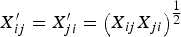 $X_{ij}^{\prime} = X_{ji}^{\prime} = {\left( {{X_{ij}}{X_{ji}}} \right)^{\textstyle{1 \over 2}}}$
:
 $$X_{ij}^{\prime} = X_{ii}^{\textstyle{1 \over 2}} X_{\,jj}^{\textstyle{1 \over 2}} {\left( {1 + {\tau _{ij}}} \right)^{1 - \sigma}} $$
where all terms are as defined above, and (11) follows directly from (10).
To derive
 $\overline {{\tau _{\iota}}} $
, we set:
 $$\mathop \sum \limits_{\,j \ne i} X_{ij}^{\prime} = \mathop \sum \limits_{\,j \ne i} {\left( {1 + {\tau _{ij}}} \right)^{1 - \sigma}} X_{ii}^{\textstyle{1 \over 2}} X_{\,jj}^{\textstyle{1 \over 2}} = \mathop \sum \limits_{\,j \ne i} {\left( {1 + \overline {{\tau _{\iota}}}} \right)^{1 - \sigma}} X_{ii}^{\textstyle{1 \over 2}} X_{\,jj}^{\textstyle{1 \over 2}} $$
Solving gives:
 $$\overline {{\tau _{\iota}}} = {\left( {\displaystyle{{\mathop \sum \nolimits_{\,j \ne i} X_{ij}^{\prime}} \over {X_{ii}^{\textstyle{1 \over 2}} \mathop \sum \nolimits_{\,j \ne i} X_{\,jj}^{\textstyle{1 \over 2}}}}} \right)^{\textstyle{1 \over {1 - \sigma}}}} - 1$$
The resulting measure will be referred to in this paper as ‘average’ trade costs. It represents a model-based aggregation of trade costs across bilateral pairs that is superior to either a simple or trade-weighted average, because it is model-based (cf. simple average) and does not underweight high levels of trade costs (cf. trade-weighted average).
3. Data treatment
This section describes the main sources used in construction of our trade costs dataset, covering production and export data. We also outline the main treatments applied to the raw data in order to construct the final dataset. After assembling all components, our dataset covers up to 167 countries for the period 1995‒2012. In sectoral terms, we cover trade in agricultural products and trade in manufactured goods, as well as total goods trade (the sum of the two sectors).
To implement equation (10) in practice, we need data on the value of bilateral trade in each direction (X ij and X ji ), and data on intra-national trade in each country (X ii and X jj ). The former data are readily available from standard sources, but the latter are more difficult to obtain. Importantly, intra-national trade needs to be measured as gross shipments, not value added, as that is the same basis on which trade values are measured. Our approach, discussed in more detail below, is to use national accounts data and to proxy intra-national trade by total production less total exports. To deal with missing observations, we use linear interpolation to calculate trade costs for country-sector-year combinations where the dataset contains missing values. Given that we are interested primarily in the developing country context, there is a necessarily a certain degree of measurement error in our data. However, as Novy (Reference Novy2013) demonstrates, our methodological approach is quite robust to reasonable assumptions concerning measurement error.
3.1 International trade data
Our bilateral trade data are sourced from the WITS-Comtrade database. We use reported export data because the model is couched in terms of export values. However, all results are robust to the use of inverse (mirror) data instead. The original data are reported in the 1988/1992 Harmonized System classification scheme, and we convert them to the ISIC Rev. 3 classification using a concordance. Total trade represents the total of agriculture and manufactured goods exports, whereas agriculture represents the total of ISIC sectors A and B and manufactured products cover ISIC sector D. These definitions correspond to the relevant sectoral definitions in the national accounts. Activities such as mining are therefore excluded from our analysis. All trade data are expressed in value terms in nominal US dollars, so no further conversions are necessary.
The main issue that arises in our trade data is in relation to re-exports. To apply equation (10), we need each country's ‘true’ (i.e., net) exports. Our dataset is therefore based on Comtrade's reported net exports for each country pair, but we are aware that not all countries properly account for re-exports in the original data. In 2012, for example, only 15% of country pairs reported bilateral re-exports for total trade. Many of these instances of missing observations in fact represent zeros, but it is not always the case.Footnote 2
3.2 Gross output and value added data
The most challenging part of this exercise from a data point of view is obtaining information on gross domestic usage, i.e. production made and sold within each country. Our starting point is the United Nations National Accounts Database. That source provides total output on a gross shipments basis disaggregated by ISIC sector for up to 137 countries. We use these data whenever available, converting them to US dollars using the nominal exchange rate applied by the World Development Indicators to convert GDP from local currency into US dollars.
When gross output data are unavailable, we take an alternative approach. We obtain data on value added by ISIC aggregate – agriculture and manufactures – from the World Development Indicators, in US dollars. Where value added data are missing from the World Development Indicators, we fill them in using the UN National Accounts Database, converting from local currency to US dollars in the same way as above. Value added data cannot be directly used in the calculation of trade costs because they net out intermediate goods and therefore tend to understate the level of production. We therefore apply a scaling up factor equal to the average sectoral ratio between value added and gross output for those countries where both sets of data are available in any given year. The annual ratios we find in the data range from 1.74 to 1.93 for agriculture, and from 3.08 to 3.75 for manufacturing. Multiplying these ratios by the value added data allows us to produce estimated gross output data for the remaining countries in our dataset. In all cases, we compute total gross output as the sum of manufactured goods and agriculture.Footnote 3
The final stage in the treatment of these data is to calculate the value of domestic production usage, i.e. intra-national trade. To do this, we follow the existing literature in taking the gross output data – actual and estimated – and subtracting the total value of exports to the rest of the world from the Comtrade data, to give the amount of total production that was both made and consumed domestically.
3.3 Parameter assumptions
As noted above, calculations of the level of trade costs are sensitive to the choice of parameter value for the intra-sectoral elasticity of substitution. We follow Novy (Reference Novy2013) in assuming that the elasticity is constant across sectors, countries, and years.Footnote 4 In all calculations, we therefore set it equal to 8, which represents about the mid-point of available estimates. In any case, as noted above, it is essentially the level of ad valorem equivalent trade costs that is sensitive to this assumption. It has hardly any impact on inferences we draw as to changes in trade costs across countries and time periods. In particular, as Novy (Reference Novy2013) shows, index numbers based on the trade costs ratio – on which our analysis focuses – are relatively insensitive to the choice of parameter assumption.
4. Results and discussion
4.1 Descriptive analysis
To give an idea of the evolution of trade costs in the developing world over recent years, we examine average trade costs by World Bank income group and region, following the methodology set out above. In doing so, we are careful to use a constant balanced sample for all calculations, i.e. we only include country-sector combinations for which trade costs can be calculated or interpolated for all years in the sample.Footnote 5 To maximize the number of countries included in this way – 76 for manufactured goods and 91 for agriculture – we eliminate the first and last years of the full sample to focus on the period from 1996 to 2010. Finally, we avoid additional composition effects by using the current (2014) World Bank income group classification and applying it to all years in the sample.Footnote 6 China, for example, is thus considered an upper middle income country for the full sample period, although it belonged to a different group at the beginning of the sample.
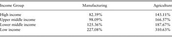
Table 1 presents average ad valorem equivalent trade costs by World Bank income group for 2010, to give an idea of the current relative levels of trade costs observed around the world. All calculations are based on the formula in equation (13).Footnote 7 Three patterns are apparent. First, trade costs in agriculture are much higher than in manufacturing, typically in the range of 50% higher to double. This finding is consistent with the fact that agricultural trade remains subject to more trade restrictions, and higher tariffs, than does trade in manufactured goods. The second broad finding to emerge from Table 1 is that trade costs in both sectors are decreasing in per capita income: there is a strict ordering from lowest trade costs (high income) to highest (low income). This finding is consistent with the historically greater degree of liberalization that has taken place in developed countries. We note that the finding stands even though trade costs as we measure them are a ratio with intra-national trade costs in the denominator, and they are typically higher in developing than in developed countries. Third, and related to the second point, is that the most striking contrast in terms of the level of trade costs is between the low income countries and the other groups, rather than among the other groups. The difference between trade costs in manufacturing for low and lower middle income countries is just over 80%, whereas the difference between the lower middle income group and the high income group is around 50%. It is therefore clear that trade costs are generally higher in the developing world than in the developed world, but that the problem is particularly severe for the poorest developing countries.
Trade costs in ad valorem equivalent terms, by sector and World Bank income group, 2010

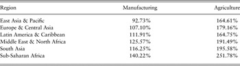
To expand on this point, Table 2 presents trade costs for 2010 by World Bank region. These regions exclude high income countries, i.e. they are limited to developing countries only (taking a broad definition of that term). There is considerable evidence of heterogeneity across developing country regions. For manufacturing, the level of trade costs in East Asia and the Pacific in 2010 was 93%, a number that was not too much higher than the high income average (82%). By contrast, Sub-Saharan Africa had average trade costs of 140%, or more than 50% higher than the East Asia and the Pacific result. Again, Table 2 shows that trade costs in agriculture are much higher than in manufacturing, a result that holds across all regions; however, the finding depends to some degree on the assumption of a common elasticity of substitution for both sectors. In particular, in the approach we have adopted it is difficult to disentangle pure differences in trade costs from differences in preferences that lead to greater or lesser tradability of certain commodities, an issue that is of particular importance in agriculture where some products tend to be traded only locally. Although trade costs might be part of the story behind that pattern of production and consumption, preferences also play a role. As a result, it is necessary to interpret our finding on the difference between trade costs in agriculture and manufacturing with appropriate caution.
Trade costs in ad valorem equivalent terms, by sector and World Bank developing country region, 2010

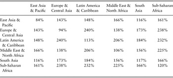
Table 3 analyzes a different split of the data. It uses our aggregation technique described in Section 2 to calculate intra- and extra-regional trade costs. The diagonal of the table is intra-regional trade costs in ad valorem equivalent terms, and the off diagonal elements are extra-regional trade costs. A number of findings stand out. First, intra-regional trade costs are generally much lower than extra-regional trade costs, as is to be expected. The exception is South Asia, where the two are roughly equivalent. This finding sits well with anecdotal evidence to the effect that it is often more cost effective to ship goods via Singapore than it is to send them directly between two points in South Asia. Second, intra-regional trade costs in East Asia and the Pacific are the lowest of any region; those in Sub-Saharan Africa are highest, at about 40% more than the East Asia and the Pacific number. Third, extra-regional trade costs with East Asia and the Pacific, or Europe and Central Asia, are typically the lowest observed region by region. In interpreting this result, it is important to recall that our trade costs measure is bilateral (the geometric average of costs to export and costs to import). As a result, the consistency of East Asia and the Pacific's results suggests that it is primarily trade cost reductions there, the benefits of which accrue in part to other regions, which are driving the results. By contrast, trade costs between some other regions can be very high, up to around 240% in the cases of Sub-Saharan Africa-Europe and Central Asia trade, and Latin America and the Caribbean‒Europe and Central Asia trade. The bilateral nature of the measure is again important in interpreting these results. Although high trade costs in Latin America and the Caribbean and Sub-Saharan Africa tell part of the story, it is also the case that many Central Asian countries are landlocked, and therefore subject to high trade costs themselves, as shown above.
Regional trade costs matrix for manufactured goods, ad valorem equivalent terms, by World Bank developing country region, 2010

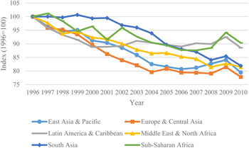
As noted in the methodological discussion above, the ad valorem equivalents presented in Table 1 are sensitive to parameter choice. Novy (Reference Novy2013), however, shows that indices based on our measure of trade costs are largely invariant to the initial choice of parameter. To examine trends over time, we therefore use index numbers. For each group of interest, we set the index equal to 100 at the beginning of the sample (1996), and then proceed to calculate changes through time for each group, and compare the resulting indices across groups. In doing so, it is very important to recall the different baselines from which different country groups start. The use of a common benchmark of 100 in 1996 is designed to make it possible to compare changes over time across groups, and does not suggest an equal level of trade costs for all groups at the beginning of the sample. In the interest of brevity, we focus on trade in manufactured goods from this point onwards.
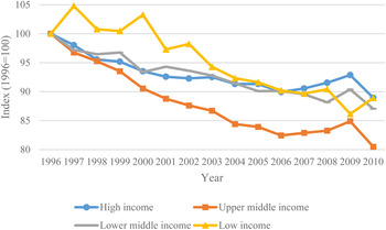
Figure 1 presents results by World Bank income group. The figure is notable for the relatively similar end points reached by three of the four groups. In other words, the high income, lower middle income, and low income groups have all seen relative reductions in trade costs that are approximately similar over the course of the sample period, albeit with a noticeable lag in the case of the low income countries. In all three cases, the country groups in question have seen trade cost reductions on the order of 12% over the sample period. Of course, the baselines and end points are very different in ad valorem equivalent terms, as demonstrated by the previous discussion. The net result of the two pieces of analysis taken together is that developing country trade costs are higher than those in developed countries, and generally are not declining any faster. This finding suggests that trade costs continue to represent a serious impediment to increased integration of developing countries into the world trading system.
Trade costs indices for manufactured goods, by World Bank income group, 1996 = 100

The obvious exception to the pattern discussed in the previous paragraph is the upper middle income group. Trade costs in that group have fallen noticeably faster than in the high income countries. This finding is consistent with the emergence of important middle income trading economies, such as Brazil, China, and South Africa, and the increasing importance of South‒South trade (Kowalski and Shepherd, Reference Kowalski and Shepherd2005; Hanson, Reference Hanson, Haddad and Shepherd2011). Our data are suggestive of a significant difference in experience across developing countries: those in the upper middle income group are catching up and increasing their level of integration into the global trading system, as their trade costs are falling faster than in high income countries (although they started from, and remain at, higher absolute levels than those countries). That is not true of any other developing country group.
Figure 2 breaks the results out by World Bank region, again excluding high income countries from the analysis. It discloses two groups of developing countries. The first – South Asia, East Asia and the Pacific, the Middle East and North Africa, and Europe and Central Asia – has seen relatively rapid reductions in trade costs, on the order of 15%‒20% over the sample period. The second group, Latin America and the Caribbean and Sub-Saharan Africa, has seen much slower falls in trade costs, of only around 10%. Of course, the baseline and end point for each region is significantly different, as discussed above, but the dynamic is nonetheless interesting. The figure strongly suggests that developing countries in some regions have been more successful than others in reducing trade costs in relative terms. In addition to the split between upper middle income countries and other developing countries referred to in the previous paragraph, this figure discloses a different dynamic path for trade costs in some developing regions as opposed to others. Of particular concern is the situation of Sub-Saharan Africa, given the development challenges it faces, and its stated desire to increase integration into the world trading system. Based on the data presented here, Sub-Saharan Africa is losing ground in relative terms to other developing country regions.
Trade costs indices for manufactured goods, by World Bank developing country region, 1996 = 100

Another important development issue in which trade costs play a role is the position of landlocked developing countries. Those countries are hampered in their integration into the global trading system by the need to rely on transit connections through third countries to access global markets. They therefore depend for their trade relations not only on the state of their own infrastructure and regulations, but on the state of those variables in neighboring countries – in addition to the application of specific rules regarding freedom of transit. It is therefore useful to break out the data for developing countries into landlocked and coastal countries.
The data tell a striking story in this case. In 2010, trade costs in manufactured goods for coastal developing countries were 123%, but they were 163% for landlocked developing countries, or nearly one-third higher. More importantly, the dynamics of trade costs over time indicate that severe problems persist for landlocked developing countries. Whereas coastal countries decreased their trade costs by nearly 25% over the sample period – from an already lower level – the corresponding change in landlocked countries was just over 10%. Despite the many initiatives that have been undertaken with regards to the special position of landlocked developing countries, there is still good reason to believe they are at a special disadvantage when it comes to trade integration, and that disadvantage is getting worse, not better, in relative terms over time, although the absolute position is improving.
4.2 Determinants of trade costs
In addition to providing descriptive statistics showing the pattern of trade costs across countries and through time, our dataset can also be used to examine the factors that contribute to the levels of trade costs observed around the world. We follow Chen and Novy (Reference Chen and Novy2011) in using a regression approach to analyze the determinants of bilateral trade costs. We include a wide range of variables familiar from the gravity model literature, covering both policy and ‘natural’ factors. As in Chen and Novy (Reference Chen and Novy2011), we focus on factors that are primarily sources of international, as opposed to domestic, trade costs.Footnote 8 One of our variables, the Logistics Performance Index, is available for 2007, 2010, 2012, and 2014; since trade costs data are not available for 2014, we limit the sample to a panel consisting of country-pair dyads for the first three years.
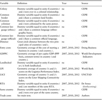
Full details of data and sources are in Table 4. Our trade costs data are symmetric, so we drop half of the sample observations to avoid understated standard errors stemming from country pair repetition. The trade costs index provides a geometric average of trade costs in both directions, so we transform the independent variables that are country specific so that they vary bilaterally. We achieve that by taking the logarithm of the geometric average of the exporter and importer values. Regression results are presented for manufactured goods only. Belgium, the Netherlands, and Singapore are excluded from the estimation sample due to the issues with re-exports identified above.
Data and sources

Using the data set out in Table 4, our regression equation takes the following form (where e is a standard error term) and is estimated by OLS:Footnote 9
 $$\eqalign{& \log \left( {trade\; cost{s_{ij}}} \right) = {b_0} + {b_1}\log \left( {distanc{e_{ij}}} \right) + {b_2}common\; borde{r_{ij}} \cr & + {b_3}common\; language\; ethno{._{ij}} + {b_4}common\; language\; officia{l_{ij}} \cr & + {b_5}colon{y_{ij}} + {b_6}common\; colonize{r_{ij}} + {b_7}same\; countr{y_{ij}} \cr & + {b_8}landlocke{d_{ij}} + {b_9}RT{A_{ij}} + {b_{10}}\log (LSC{I_{ij}}) + {b_{11}}\log (LP{I_{ij}}) \cr & + {b_{12}}\log \left( {entry\; cost{s_{ij}}} \right) + {e_{ij}}} $$
where distance is the geodesic distance between the exporting and importing countries, using the largest (by population) city in each; common border is a dummy variable equal to 1 if the two countries are geographically contiguous; the two common language variables are dummies equal to 1 if the two countries share a common language, either on an ethnographic or official basis; colony is a dummy variable equal to 1 if one of the countries was once a colony of the other; common colonizer is a dummy variable equal to 1 if the two countries were once colonized by the same power; same country is a dummy equal to 1 if the two countries were once part of the same country; landlocked is a dummy variable equal to 1 if either country is landlocked; RTA is a dummy variable equal to 1 if there is a regional trade agreement in force between the two countries; LSCI is the UNCTAD Liner Shipping Connectivity Index, as a proxy for international transport connectivity;Footnote 10 LPI is the World Bank Logistics Performance Index, as a proxy for trade facilitation performance; and entry costs are the cost of starting a business, from the World Bank's Doing Business project, as a proxy for the costs of market entry.
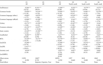
Regression results are in Table 5, with baseline results in column 1. All of the geographical variables have parameters with the expected signs and statistical significance, and sensible magnitudes. For example, a 10% increase in the distance between two countries is associated with a nearly 3% increase in trade costs. This coefficient is smaller than in typical gravity regressions where the dependent variable is trade flows, rather than trade costs, because parameter estimates in standard gravity conflate the elasticity of trade costs with respect to distance and the intrasectoral elasticity of substitution. Assuming an elasticity of eight, as above, the implied coefficient for the elasticity of trade flows with respect to distance is 2.0, which is somewhat high. However, the difference from traditional gravity estimates is perhaps not surprising when it is considered that our approach relies on a transformation of the trade data, and covers a wide variety of products and countries. In any case, the implied distance elasticity is sensitive to the choice of intra-sectoral elasticity of substitution, which is subject to considerable uncertainty.
Regression results

Note: The dependent variable is log(trade costs) for manufactured goods in all cases. Estimation is by OLS. T-statistics based on robust standard errors adjusted for clustering by country pair appear in parentheses below the parameter estimates. Statistical significance is indicated by: * (10%), ** (5%), and *** (1%).
The first trade policy variable of interest is the RTA dummy. It is negatively signed, and statistically significant at the 1% level. By exponentiation, countries that are both members of an RTA exhibit trade costs that are around 16% lower than those that are not. Comparing this result with the distance elasticity suggests that policy is extremely important for trade costs: existence of an RTA is equivalent to reducing bilateral distance by around 50%. Signing RTAs may therefore be an effective way of inducing reductions in bilateral trade costs among partners, although we are careful not to draw any normative conclusions about welfare because of the possibility of trade diversion, which cannot be captured in this kind of model.
The LSCI and the LPI both have negative parameters that are statistically significant at the 1% level. Improvements of 10% in these indices are associated with 2.5% and 16.2% reductions in trade costs respectively. Again, these are economically significant numbers, which suggest that international transport connectivity and trade facilitation performance can be effective levers in reducing trade costs.
The final policy variable, Doing Business market entry costs as a proxy for the fixed costs of entering a foreign market, has the expected positive coefficient estimate that is statistically significant at the 1% level. However, the magnitude of the effect is relatively small: a 10% decrease in market entry costs is associated with a 0.2% decrease in trade costs.
A limitation of the baseline results is that they do not exploit the panel nature of the dataset to control for unobserved heterogeneity that could be driving trade costs. Column 2 accounts for this possibility by including exporter, importer, and year fixed effects.Footnote 11 While it is important to estimate this model as a robustness check, its structure means that we must exclude the bilateralized policy variables because they are collinear with the fixed effects in this log-log model. Results on the remaining variables are remarkably stable to the introduction of fixed effects: the coefficients on the geographical variables and the RTA dummy change only slightly, and always retain their signs and statistical significance. We can therefore be confident that our results are not being driven by unobserved heterogeneity by importer, exporter, or time period.
An additional limitation of the baseline results is that they do not account for per capita income effects (development level). It could be argued that a country's level of development is strongly correlated with policy variables, and thus its omission could lead to biased estimates. Column 3 of Table 5 shows that that contention does not hold up. Results are almost identical to column 1, and the coefficients on per capita GDP are statistically insignificant. It is therefore highly unlikely that income effects are driving the associations we have observed in the data between policy variables and trade costs.
The regression results presented in the first three columns of Table 5 pool all countries together. As a result, they do not take account of the specificity of different types of trade relations, such as those between countries at different levels of development. To investigate whether this issue makes any difference to the results, the last three columns of Table 5 present regression results for split samples. Using the World Bank's country classification, countries are divided into the ‘North’ (high income countries) and the ‘South’ (low and middle income countries), and regressions with bilateralized policy variables are estimated separately for each sample.
Results for the geographical variables are reasonably consistent across the last three columns of Table 5 in terms of magnitude, sign, and statistical significance. Common ethnographic language only has a statistically significant coefficient for North–North and South–North trade, while the colony dummy unsurprisingly has a statistically insignificant coefficient for South–South trade, as does the dummy variable for countries that were once part of the same country.
Results for the policy variables are interesting. The RTA dummy has a negative and statistically significant coefficient in all three regressions, but its magnitude changes noticeably: North–North and South–South RTAs tend to reduce trade costs more than do North–South RTAs. This finding may be indicative of a lack of ambition or coverage in North–South RTAs, or the fact that they are sometimes unbalanced in terms of the effective liberalization undertaken, in the sense that the Southern partner may benefit from very long phase-in periods.
As in the baseline regression, the LSCI has a negative and statistically significant coefficient in all three models, and magnitudes are relatively similar in the three cases.
The LPI also has negative and statistically significant coefficients in all three regressions. However, the absolute value of the coefficient is largest in the South–South regression. This finding indicates that logistics and trade facilitation are particularly important for South–South trade.
5. Conclusion and policy implications
In this paper, we have used newly collected data on international trade and production to infer estimates of trade costs for up to 167 countries over the period 1995–2012. Our estimates distinguish between trade in manufactured goods and trade in agricultural products. In both cases, we find that absolute levels of trade costs are highly significant in ad valorem equivalent terms, ranging from an average of just over 80% for high income countries in manufactures, to over 300% for low income countries in agriculture. Our results suggest that although the international economy has integrated considerably in recent decades, there remain potentially large unexploited gains to be reaped from further reducing the wedge between export and import prices.
From a policy point of view, our results are significant because they show that trade costs fall disproportionately on developing countries. Low income countries face high absolute levels of trade costs, but their relative position has not been improving in recent years. Only the upper middle income countries have succeeded in reducing trade costs at a faster rate than other income groups, albeit from a higher starting point. Similarly, we find considerable geographical disparity among developing countries with some regions – particularly East Asia and the Pacific – exhibiting much lower levels of trade costs than others, such as Sub-Saharan Africa.
In addition to mapping out the level and direction of change of trade costs in the developing world over recent decades, we have used econometric methods to decompose trade costs into various policy and geographical/historical components. Our findings clearly suggest that policy matters for trade costs. Initiatives such as regional trade agreements, improving transport connectivity, and, in some cases, boosting trade facilitation performance are important ways of reducing trade costs. The relative effectiveness of these policy levers differs according to the country income group under consideration, which means that a differentiated approach may be appropriate.
In interpreting our results, it is important to keep in mind that our trade costs estimates are model-based, and therefore depend on a series of assumptions. Although the general framework within which our approach can be applied is broad – any model that produces a gravity model with importer and exporter fixed effects can be manipulated in the same way – it is possible that future work using different theoretical assumptions will lay stress on other factors that lead to observed changes in the pattern of trade and production. One issue future research can usefully examine is the role value chains play in contemporary trade, and the interaction between trade costs and other factors influencing firm sourcing decisions that the business model implies.
Appendix: Descriptive statistics for the regression sample