1. Introduction
Balance control of quadruped robots has a significant impact on stable and fast locomotion [Reference Gor, Pathak, Samantaray, Yang and Kwak1]. Balance control algorithms have been studied for several decades, which were verified with quadruped robots under different gaits [Reference Biswal and Mohanty2]. Mainstream algorithms include Model Predictive Control (MPC), Whole Body Control (WBC), Central Pattern Generator (CPG), Virtual Model Control (VMC), and Zero Moment Point (ZMP), which achieve balance control for quadruped robots successfully. However, the algorithms mentioned have their limitations. MPC, WBC, and CPG all involve complex mathematical calculations and parameter adjustments. Pure VMC limits the most accurate balance control to some extent. ZMP is not conducive to balance control for dynamics.
MPC is a method to calculate forces of supporting foot in each controlling cycle by model prediction and convex optimization [Reference Di Carlo, Wensing, Katz, Bledt and Kim3]. The MPC process includes the establishment of state-space expressions, predictions of several future states based on current states, creation of Quadratic Programming (QP) expression combining prediction states and planned trajectory, weights distribution about states and input parameters, and solution of the cost function [Reference Bledt, Powell, Katz, Di Carlo, Wensing and Kim4, Reference Horvat, Melo and Ijspeert5]. The forces calculated can be converted to joint torques by the Jacobian matrix. MPC achieves body balance control during high-speed locomotion, which simultaneously considers the whole states of the robot, adjusting weights to control some critical states [Reference Rutschmann, Satzinger, Byl and Byl6–Reference Wieber8]. However, the solving process of the cost function is complex due to enormous prediction states and iterations, resulting in a long calculating period. What is more difficult is that modulation of any weight will influence other states, which demands the high accuracy of robotic physical parameters.
WBC is a method considering the control of all body states [Reference Saab, Ramos, Keith, Mansard, Soueres and Fourquet9]. WBC divides control tasks and assigns different priorities to realize the overall control due to the strong coupling system [Reference Kim, Jorgensen, Lee, Ahn, Luo and Sentis10, Reference Saputra, Ijspeert and Kubota11]. Pseudo-inverse operation is carried out on Jacobian matrix based on null space method, and tasks with lower priority are filtered by multiplying pseudo-inverse matrix and original matrix, ensuring the execution of tasks with higher priority [Reference Lee, Hwang and Park12]. WBC based on quadratic programming (QP) considers all dynamic states by assigning the same priorities to each task [Reference Kuindersma, Permenter and Tedrake13]. However, only WBC will lose accurate control on the states with lower priority while controlling the states with higher priority.
CPG is a distributed neural network control method based on animal movement rhythm [Reference Ijspeert14, Reference Wu, Liu, Zhang and Chen15]. Neural vibrators are designed on each joint according to the distribution principle, the neural vibrators are associated with each other according to the overall robot structure, and feedback signals from external sensors are imported simultaneously. Each neural oscillator outputs specific waveforms related to joint angle, joint velocity, and joint torque to control joint motions based on upper motion planning, feedback information, and other neural oscillator status signals. CPG connects each joint of the robot and introduces feedback mechanisms, which improve the terrain adaptability and dynamic balancing ability of the robot. The distributed neural oscillator network realizes the motion control of the quadruped robot under different gaits [Reference Rutishauser, Sprowitz, Righetti and Ijspeert16, Reference Billard and Ijspeert17] and adjusts the corresponding model parameters during the motion to finish the smooth transition of different gaits while flexibly performing the all-around motion such as side shift and turn [Reference Nagashino, Nomura and Kinouchi18–Reference Santos and Matos20]. However, upper control tasks are converted into joint instructions through multiple links, which occupies a large number of computing resources of the computer, resulting in a long control cycle and low task execution efficiency.
VMC provides virtual forces and torques by exerting fictitious spring or damping on the center of mass (CoM) [Reference Raibert and Tello21–Reference Raibert23]. The forces and torques can be adjusted by changing the stiffness coefficient and damping coefficient. Horizontal virtual forces control forward and lateral movement, vertical virtual force controls the altitude of the body, and virtual torques control the attitude of the body [Reference Pratt, Chew, Torres, Dilworth and Pratt24, Reference Pratt25]. All virtual forces and torques are converted into joint torques. Many mainstream gaits, including trot, bounce, gallop, are successfully studied based on VMC criterion [Reference Marhefka, Orin, Schmiedeler and Waldron26–Reference Estremera and Waldron28]. VMC is a direct method based on intuitive control, which responds fast without complex calculations. However, pure VMC is not able to guarantee accurate control.
ZMP was first used in static balance control [Reference Yang29]. For biped robots, static and quasi-static posture balance can be achieved because the sole has a supporting area [Reference Dimas Pristovani, Rindo, Henfri, Subhan and Pramadihanto30]. For quadruped robots, at least three legs are required to maintain static balance due to the point contact [Reference Kim31]. However, the kinematic moving speed is limited. Along with the deeper study of ZMP, compensating swing trajectory is introduced to develop dynamic ZMP, keeping the CoM on the diagonal line of supporting foot by deliberately swinging the body from side to side [Reference Pongas, Mistry and Schaal32–Reference Zhiqiang, Yuanbing, Xiuli and Yun34]. Dynamic ZMP achieves balance control during slow dynamic motion by establishing ZMP region and torque compensation [Reference Prahlad, Dip and Meng-Hwee35, Reference Kalakrishnan, Buchli, Pastor, Mistry and Schaal36]. Nevertheless, it is difficult to accurately control the ZMP projection on the diagonal line due to the inertial force in the fast movement, causing the robot to fall down.
The balance control of trot gait enhances the practical applicability of quadruped robot, which involves many meaningful tasks such as global mapping and valuables handling. When the quadruped robot is equipped with radar or laser for mapping, the stable balanced attitude can suppress the vibration, reduce the dependence on filtering, and improve the mapping efficiency and accuracy [Reference Liu, Jiang, Zou, Xing, Wang and Su37]. Although the current algorithms achieve stability control, there is space for optimization to improve practicability.
Therefore, this paper proposes a six-dimensional spatial mechanics decoupling algorithm. The algorithm describes and solves the mathematic relationship between six ground reaction forces of the diagonal supporting leg and six spatial forces and torques controlling robot degrees of freedom (DoF), achieving body balance control during trot gait. VMC with impedance control is applied to CoM to analyze the virtual forces and torques. A matrix
 $ \in {\mathbb{R}}^{6\times 6}$
is established to describe the relationship between ground reaction forces and virtual forces and torques. The ground reaction forces are then calculated by matrix inversion, and forces are converted to joint torques through the Jacobian matrix. However, the initial matrix fails to reach full rank due to the physical structure of the quadruped robot itself. The maximum rank of the matrix is five, so some physical parameters in the matrix should be amended by temporarily sacrificing the accurate control of one of the six DoFs. VMC with impedance control is also applied to the swinging foot, and the foot trajectory is generated through cubic interpolation. In addition, if accurate control of locomotive speed is sacrificed, the selection of landing point of swing leg should be considered for adjusting the velocity effectively. Moreover, an intervention control method based on center of mass (CoM) projection is introduced to regulate locomotive speed. Advantages of the theoretical algorithm proposed in this paper include the following:
-
1. small amount calculation without iteration calculations,
-
2. high accuracy of balance control, and
-
3. newly available adjusting method of locomotive velocity.
This paper is organized into the following section to address. In Section 2, the six-dimensional spatial mechanics matrix and solution are described in detail. In Section 3, locomotive velocity adjustment based on selection of landing point and region intervention control (RIC) are described in detail. In Section 4, simulations are launched to verify the feasibility of the proposed algorithm with and without intervention control in Webots software. In Section 5, relative conclusions are drawn to summarize the effectiveness of the algorithm. In Section 6, further outlooks about balance control are discussed.
2. Six-Dimensional Spatial Mechanics Matrix and Solution
2.1. Convention
Matrix
 $ \in {\mathbb{R}}^{n\times m}$
is represented with uppercase, upright, and bold letter(A). Matrix
 $ \in {\mathbb{R}}^{n\times 1}/{\mathbb{R}}^{1\times n}$
is represented with uppercase, italicized, and bold letter(
A
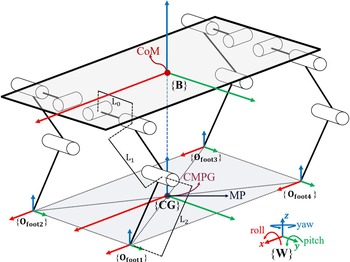
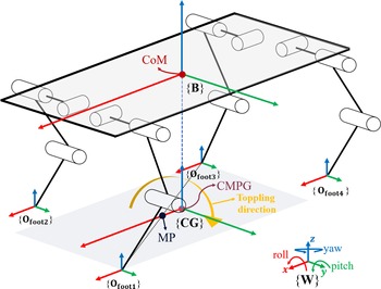
). Scalar is represented with uppercase or lowercase and upright letter(A, a). This paper includes four different coordinates, as shown in Fig. 1, and symbols in different coordinates will attach an identifier on them. As an example, all quantities in the body coordinate system have a left subscript B(
 $^{\textrm{B}}\textrm{A}$
). Coordinate is represented with an uppercase, upright, and bold letter within brace({A}).
Coordinates systems. {W} is world coordinate, which works as a reference coordinate. {B} is a body coordinate, which is established in CoM. {CG} is a coordinate established in the point where CoM is projected on the ground. {Ofooti} is a coordinate established in the foot of each leg. L0 is the length from hip roll joint axis to hip pitch joint axis. L1 is the length of upper leg. L2 is the length of lower leg.

2.2. Model of quadruped robot and analysis of six-dimensional spatial mechanics
As shown in Fig. 1, the research in this paper is conducted based on a quadruped robot with twelve DoFs, including four legs. Leg 1, leg 2, leg 3, and leg 4 correspond to left front leg, right front leg, right hind leg, and left hind leg, respectively. Every leg has three DoFs, including hip roll DoF, hip pitch DoF, and knee pitch DoF. The robot itself has six DoFs, including three translational DoFs and three rotational DoFS [Reference Kazemi, Majd and Moghaddam38]. Four coordinates are used for describing various physical quantities and state quantities. The main task of the paper is to maintain body balanced during trot gait, so the orientation of the four coordinates is identical. The unique posture shown in Fig. 1 indicates that CoM projected on the ground (CMPG) overlaps the middle point (MP) in the line connecting foot 1 and foot 3 or the line connecting foot 2 and foot 4. The posture is considered as the most balanced state, and the positions of feet in {B} are recorded.
 \begin{align}^{\bf{B}}{{\bf{P}}_{{\bf{footi}}}} = {{[^{\textrm{B}}}{{\textrm{O}}_{{\textrm{fxi}}}}{\,^{\textrm{B}}}{{\textrm{O}}_{{\textrm{fyi}}}}\,{\,^{\textrm{B}}}{{\textrm{O}}_{{\textrm{fzi}}}}]^{\textrm{T}}}\end{align}
where i stands for leg i.
 $^{\textrm{B}}{\textrm{O}}_{\textrm{f}\textrm{*}\textrm{i}}$
are positions of foot coordinate origin in x, y, and z directions in body coordinate.
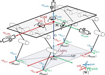
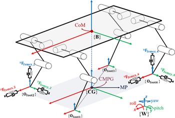
As shown in Fig. 2, the ground reaction forces are distributed in each foot. According to VMC criterion, the robot is considered as a rigid body with the mass of four legs much less than the total mass, so the ground reaction forces can be equivalent to acting on the CoM [Reference Di Carlo, Wensing, Katz, Bledt and Kim3]. Therefore, the virtual forces and torques are generated from ground reaction forces.
 \begin{align} {}_{}{}^{B}{F}_{CoM}=\textrm{}{\textrm{}\left[{}_{\textrm{}}{}^{\textrm{B}}{\textrm{F}}_{\textrm{C}\textrm{o}\textrm{M}\textrm{x}\textrm{}\textrm{}}\textrm{}{{}_{\textrm{}}{}^{\textrm{B}}{\textrm{F}}_{\textrm{C}\textrm{o}\textrm{M}\textrm{y}\textrm{}\textrm{}}}_{\textrm{}\textrm{}}{}_{\textrm{}}{}^{\textrm{B}}{\textrm{F}}_{\textrm{C}\textrm{o}\textrm{M}\textrm{z}\textrm{}\textrm{}}\textrm{}{}_{\textrm{}}{}^{\textrm{B}}{\textrm{}\textrm{T}}_{\textrm{C}\textrm{o}\textrm{M}\textrm{x}\textrm{}\textrm{}}{}_{\textrm{}}{}^{\textrm{B}}{\textrm{}\textrm{T}}_{\textrm{C}\textrm{o}\textrm{M}\textrm{y}\textrm{}\textrm{}}{}_{\textrm{}}{}^{\textrm{B}}{\textrm{}\textrm{T}}_{\textrm{C}\textrm{o}\textrm{M}\textrm{z}\textrm{}\textrm{}}\right]}^{\textrm{T}}\end{align}
Ground reaction forces and virtual forces and torques.

where
 $^{\textrm{B}}{\textrm{F}}_{\textrm{C}\textrm{o}\textrm{M}\textrm{}\textrm{}}$
and
 $^{\textrm{B}}{\textrm{}\textrm{T}}_{\textrm{C}\textrm{o}\textrm{M}\textrm{}\textrm{}}$
are virtual forces and torques in body coordinate, respectively.
 \begin{align} \left\{\begin{array}{@{}l}{}_{\textrm{}}{}^{\textrm{B}}{\textrm{F}}_{\textrm{C}\textrm{o}\textrm{M}\textrm{x}\textrm{}\textrm{}}={}_{\textrm{}}{}^{\textrm{W}}{\textrm{F}}_{\textrm{C}\textrm{o}\textrm{M}\textrm{x}}={\textrm{K}}_{\textrm{p}\textrm{x}}\!\left({}_{\textrm{}}{}^{\textrm{W}}{\textrm{P}}_{\textrm{X}\textrm{C}\textrm{o}\textrm{M}\_{\textrm{d}}}-{}_{\textrm{}}{}^{\textrm{W}}{\textrm{P}}_{\textrm{X}\textrm{C}\textrm{o}\textrm{M}}\right)+{\textrm{B}}_{\textrm{p}\textrm{x}}({}_{\textrm{}}{}^{\textrm{W}}{\textrm{V}}_{\textrm{X}\textrm{C}\textrm{o}\textrm{M}\_{\bf{d}}}-{}_{\textrm{}}{}^{\textrm{W}}{\textrm{V}}_{\textrm{X}\textrm{C}\textrm{o}\textrm{M}})\\ \\[-7pt] ^{\textrm{B}}{\textrm{F}}_{\textrm{C}\textrm{o}\textrm{M}\textrm{y}\textrm{}\textrm{}}={}_{\textrm{}}{}^{\textrm{W}}{\textrm{F}}_{\textrm{C}\textrm{o}\textrm{M}\textrm{y}}={\textrm{K}}_{\textrm{p}\textrm{y}}\!\left({}_{\textrm{}}{}^{\textrm{W}}{\textrm{P}}_{\textrm{Y}\textrm{C}\textrm{o}\textrm{M}\_{\bf{d}}}-{}_{\textrm{}}{}^{\textrm{W}}{\textrm{P}}_{\textrm{Y}\textrm{C}\textrm{o}\textrm{M}}\right)+{\textrm{B}}_{\textrm{p}\textrm{y}}({}_{\textrm{}}{}^{\textrm{W}}{\textrm{V}}_{\textrm{Y}\textrm{C}\textrm{o}\textrm{M}\_{\bf{d}}}-{}_{\textrm{}}{}^{\textrm{W}}{\textrm{V}}_{\textrm{Y}\textrm{C}\textrm{o}\textrm{M}})\\ \\[-7pt] ^{\textrm{B}}{\textrm{F}}_{\textrm{C}\textrm{o}\textrm{M}\textrm{z}\textrm{}\textrm{}}={}_{\textrm{}}{}^{\textrm{W}}{\textrm{F}}_{\textrm{C}\textrm{o}\textrm{M}\textrm{z}}={\textrm{K}}_{\textrm{p}\textrm{z}}\!\left({}_{\textrm{}}{}^{\textrm{W}}{\textrm{P}}_{\textrm{Z}\textrm{C}\textrm{o}\textrm{M}\_{\bf{d}}}-{}_{\textrm{}}{}^{\textrm{W}}{\textrm{P}}_{\textrm{Z}\textrm{C}\textrm{o}\textrm{M}}\right)+{\textrm{}\textrm{B}}_{\textrm{p}\textrm{z}}({}_{\textrm{}}{}^{\textrm{W}}{\textrm{V}}_{\textrm{Z}\textrm{C}\textrm{o}\textrm{M}\_{\bf{d}}}-{}_{\textrm{}}{}^{\textrm{W}}{\textrm{V}}_{\textrm{Z}\textrm{C}\textrm{o}\textrm{M}})-mg\\ \\[-7pt] ^{\textrm{B}}{\textrm{T}}_{\textrm{C}\textrm{o}\textrm{M}\textrm{x}}={}_{\textrm{}}{}^{\textrm{W}}{\textrm{T}}_{\textrm{C}\textrm{o}\textrm{M}\textrm{x}}={\textrm{K}}_{{\theta }\textrm{x}}\!\left({}_{\textrm{}}{}^{\textrm{W}}{{\theta }}_{\textrm{X}\textrm{C}\textrm{o}\textrm{M}\_{\bf{d}}}-{}_{\textrm{}}{}^{\textrm{W}}{{\theta }}_{\textrm{X}\textrm{C}\textrm{o}\textrm{M}}\right)+{\textrm{B}}_{{\theta }\textrm{x}}({}_{\textrm{}}{}^{\textrm{W}}{{\omega }}_{\textrm{X}\textrm{C}\textrm{o}\textrm{M}\_{\bf{d}}}-{}_{\textrm{}}{}^{\textrm{W}}{{\omega }}_{\textrm{X}\textrm{C}\textrm{o}\textrm{M}})\\ \\[-7pt] ^{\textrm{B}}{\textrm{T}}_{\textrm{C}\textrm{o}\textrm{M}\textrm{y}}={}_{\textrm{}}{}^{\textrm{W}}{\textrm{T}}_{\textrm{C}\textrm{o}\textrm{M}\textrm{y}}={\textrm{K}}_{{\theta }\textrm{y}}\!\left({}_{\textrm{}}{}^{\textrm{W}}{{\theta }}_{\textrm{Y}\textrm{C}\textrm{o}\textrm{M}\_{\bf{d}}}-{}_{\textrm{}}{}^{\textrm{W}}{{\theta }}_{\textrm{Y}\textrm{C}\textrm{o}\textrm{M}}\right)+{\textrm{B}}_{{\theta }\textrm{y}}({}_{\textrm{}}{}^{\textrm{W}}{{\omega }}_{\textrm{Y}\textrm{C}\textrm{o}\textrm{M}\_{\bf{d}}}-{}_{\textrm{}}{}^{\textrm{W}}{{\omega }}_{\textrm{Y}\textrm{C}\textrm{o}\textrm{M}})\\ \\[-7pt] ^{\textrm{B}}{\textrm{T}}_{\textrm{C}\textrm{o}\textrm{M}\textrm{z}}={}_{\textrm{}}{}^{\textrm{W}}{\textrm{T}}_{\textrm{C}\textrm{o}\textrm{M}\textrm{z}}={\textrm{K}}_{{\theta }\textrm{z}}\!\left({}_{\textrm{}}{}^{\textrm{W}}{{\theta }}_{\textrm{Z}\textrm{C}\textrm{o}\textrm{M}\_{\bf{d}}}-{}_{\textrm{}}{}^{\textrm{W}}{{\theta }}_{\textrm{Z}\textrm{C}\textrm{o}\textrm{M}}\right)+{\textrm{B}}_{{\theta }\textrm{z}}({}_{\textrm{}}{}^{\textrm{W}}{{\omega }}_{\textrm{Z}\textrm{C}\textrm{o}\textrm{M}\_{\bf{d}}}-{}_{\textrm{}}{}^{\textrm{W}}{{\omega }}_{\textrm{Z}\textrm{C}\textrm{o}\textrm{M}})\end{array}\right.\end{align}
where
 $^{\textrm{W}}{\textrm{F}}_{\textrm{C}\textrm{o}\textrm{M}}$
and
 $^{\textrm{W}}{\textrm{T}}_{\textrm{C}\textrm{o}\textrm{M}}$
are virtual forces and torques in world coordinate, respectively.
 $ {\textrm{K}}_{\textrm{*}\textrm{*}}$
and
 $ {\textrm{B}}_{\textrm{*}\textrm{*}}$
are stiffness coefficient and damping coefficient, respectively.$
 $^{\textrm{W}}{\textrm{P}}_{\textrm{*}\textrm{C}\textrm{o}\textrm{M}}$
,
 $^{\textrm{W}}{\textrm{V}}_{\textrm{*}\textrm{C}\textrm{o}\textrm{M}}$
,
 $^{\textrm{W}}{{\theta }}_{\textrm{*}\textrm{C}\textrm{o}\textrm{M}}$
, and
 $^{\textrm{W}}{{\omega }}_{\textrm{*}\textrm{C}\textrm{o}\textrm{M}}$
are position, velocity, angle, and angular velocity of robot, respectively.$
 $^{\textrm{W}}{\textrm{P}}_{\textrm{*}\textrm{C}\textrm{o}\textrm{M}}{\_}_{\textrm{d}}$
,
 $^{\textrm{W}}{\textrm{V}}_{\textrm{*}\textrm{C}\textrm{o}\textrm{M}}{\_}_{\textrm{d}}$
,
 $^{\textrm{W}}{{\theta }}_{\textrm{*}\textrm{C}\textrm{o}\textrm{M}}{\_}_{\textrm{d}}$
, and
 $^{\textrm{W}}{{\omega }}_{\textrm{*}\textrm{C}\textrm{o}\textrm{M}}{\_}_{\textrm{d}}$
are desired position, velocity, angle, and angular velocity of robot, respectively. m is the mass of the robot, and if it carries load, m is amended to compensate the z virtual force.
 $ g$
is the gravitational acceleration, 9.81 m/
 $ {\textrm{s}}^{2}$
.
The ground reaction forces are represented as
 \begin{align} {}_{}{}^{\bf{W}}{\bf{F}}_{\bf{footi}}=\textrm{}{\textrm{}\left[{}_{\textrm{}}{}^{\textrm{W}}{\textrm{F}}_{\textrm{f}\textrm{x}\_{\bf{i}}\quad \textrm{}\textrm{}}{}_{\textrm{}}{}^{\textrm{W}}{\textrm{F}}_{\textrm{f}\textrm{y}\_{\bf{i}}\quad \textrm{}\textrm{}}{}_{\textrm{}}{}^{\textrm{W}}{\textrm{F}}_{\textrm{f}\textrm{z}\_{\bf{i}}\textrm{}\textrm{}}\right]}^{\textrm{T}}\end{align}
where
 $^{\textrm{W}}{\textrm{F}}_{\textrm{f}\textrm{*}\_{\bf{i}}}$
is ground reaction forces from x, y, and z directions of leg i.
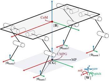
This paper focuses on balance control when only diagonal legs support the robot during trot gait. As shown in Fig. 3, the control of six virtual forces and torques is achieved by six ground reaction forces. Furthermore, virtual forces in x, y, and z axes are controlled by ground reaction forces of supporting feet in x, y, and z directions, respectively. Virtual torques around x, y, and z axes are controlled by the combined torque consisting of ground reaction forces in the other two axes. For instance, virtual torque around x axis is controlled by the combined torque consisting of ground reaction forces in y and z axes.
Diagonal legs support the robot.

The total ground reaction forces are represented as
 \begin{align} {}_{}{}^{\bf{W}}{\bf{F}}_{\bf{foot}}=\textrm{}{\textrm{}\left[{{}_{}{}^{{\bf{W}}}{{\bf{F}}}_{{\bf{footi}}}}^{T}{}{}{{}_{}{}^{\bf{W}}{\bf{F}}_{\bf{{footi+2}}}}^{T}\right]}^{\textrm{T}}={\textrm{}\left[{}_{\textrm{}}{}^{\textrm{W}}{\textrm{F}}_{\textrm{f}\textrm{x}\_{\bf{i}}\textrm{}\textrm{}}{}_{\textrm{}}{}^{\textrm{W}}{\textrm{F}}_{\textrm{f}\textrm{y}\_{\bf{i}}\textrm{}\textrm{}}{}_{\textrm{}}{}^{\textrm{W}}{\textrm{F}}_{\textrm{f}\textrm{z}\_{\bf{i}}\textrm{}\textrm{}}{}_{\textrm{}}{}^{\textrm{W}}{\textrm{F}}_{\textrm{f}\textrm{x}\_{\bf{i}}+2\textrm{}\textrm{}}{}_{\textrm{}}{}^{\textrm{W}}{\textrm{F}}_{\textrm{f}\textrm{y}\_{\bf{i}}+2\textrm{}\textrm{}}{}_{\textrm{}}{}^{\textrm{W}}{\textrm{F}}_{\textrm{f}\textrm{z}\_{\bf{i}}\textrm{}+2\textrm{}}\right]}^{\textrm{T}}\end{align}
The relationship between ground reaction forces and virtual forces and torques is established as
 \begin{align} {}_{}{}^{\bf{B}}{{\bf{F}}}_{{\bf{C}}{\bf{o}}{\bf{M}}}={\bf{\bf{M}}}_{\bf{1}}{}_{}{}^{{\bf{W}}}{{\bf{F}}}_{{\bf{f}}{\bf{o}}{\bf{o}}{\bf{t}}}\end{align}
where
 $ {\bf{M}}_{1}$
is matrix
 $ \in {\mathbb{R}}^{6\times 6}$
,
 \begin{align*} {\bf{M}}_{1}&=\left[\begin{array}{c@{\quad}c}{\bf{I}}_{\bf{i}}& {\bf{I}}_{\bf{i}+2}\\ \\[-7pt] {}_{\bf{}}{}^{\bf{B}}{\bf{D}}_{\bf{i}} &{}_{\bf{}}{}^{\bf{B}}{\bf{D}}_{\bf{i}+2}\end{array}\right]\\[4pt] {\bf{I}}_{\bf{i}}&=\textrm{}\left[\begin{array}{c}\begin{array}{c@{\quad}c@{\quad}c}1 & 0& 0\end{array}\\ \\[-7pt] \begin{array}{c@{\quad}c@{\quad}c}0& 1& 0\end{array}\\ \\[-7pt] \begin{array}{c@{\quad}c@{\quad}c}0& 0& 1\end{array}\end{array}\right] {}_{\bf{}}{}^{\bf{B}}{\bf{D}}_{\bf{i}}=\textrm{}\left[\begin{array}{c}\begin{array}{c@{\quad}c@{\quad}c}0 &-{}_{\textrm{}}{}^{\textrm{B}}{\textrm{d}}_{\textrm{z}\textrm{i}}&{}^{\textrm{B}}{\textrm{d}}_{\textrm{y}\textrm{i}}\end{array}\\ \\[-7pt] \begin{array}{c@{\quad}c@{\quad}c}{}_{\textrm{}}{}^{\textrm{B}}{\textrm{d}}_{\textrm{z}\textrm{i}}& 0& -{}_{\textrm{}}{}^{\textrm{B}}{\textrm{d}}_{\textrm{x}\textrm{i}}\end{array}\\ \\[-7pt] \begin{array}{c@{\quad}c@{\quad}c}-{}_{\textrm{}}{}^{\textrm{B}}{\textrm{d}}_{\textrm{y}\textrm{i}} &^{\textrm{B}}{\textrm{d}}_{\textrm{x}\textrm{i}} &0\end{array}\end{array}\right]\end{align*}
where
 $ {\bf{I}}_{\bf{i}}$
is diagonal matrix
 $ \in {\mathbb{R}}^{3\times 3}$
.
 $^{\bf{B}}{\bf{D}}_{\bf{i}}$
is the matrix
 $ \in {\mathbb{R}}^{3\times 3}$
containing the distances from each foot to CoM.
 $^{\textrm{B}}{\textrm{d}}_{\textrm{*}\textrm{i}}$
are positions of each foot in body coordinate.
Denavit–Hartenberg parameters are used for establishing coordinate transformation matrix.
 \begin{align} {{}_{\bf{}}{}^{\bf{j}-\bf{1}}\bf{T}}_{\bf{j}\_{\bf{i}}}=\left[\begin{array}{c@{\quad}c}{{}_{\bf{}}{}^{\bf{j}-\bf{1}}\bf{R}}_{\bf{j}\_{\bf{i}}} & {{}_{\bf{}}{}^{\bf{j}-\bf{1}}\bf{P}}_{\bf{j}\_{\bf{i}}}\\ \\[-7pt] 0\,0\,0& 1\end{array}\right]\end{align}
where
 $ {{}_{\textrm{}}{}^{\bf{j}-\bf{1}}\bf{T}}_{\bf{j}\_{\bf{i}}}$
 $ \in \textrm{}{\mathbb{R}}^{4\times 4}$
is the coordinate transformation matrix.
 $ {{}_{\textrm{}}{}^{\bf{j}-\bf{1}}\bf{R}}_{\bf{j}\_{\bf{i}}}$
and
 $ {{}_{\textrm{}}{}^{\bf{j}-\bf{1}}\bf{P}}_{\bf{j}\_{\bf{i}}}$
 $ \textrm{}\in \textrm{}{\mathbb{R}}^{3\times 3}$
are rotational and translational transformation matrixes, respectively.
The parameters of distance matrix
 $^{\bf{B}}{\bf{D}}_{\bf{i}}$
are obtained as follows:
 \begin{align} \left[\begin{array}{c}{}_{\textrm{}}{}^{\textrm{B}}{\textrm{d}}_{\textrm{x}\textrm{i}}\\ \\[-7pt] ^{\textrm{B}}{\textrm{d}}_{\textrm{y}\textrm{i}}\\ \\[-7pt] ^{\textrm{B}}{\textrm{d}}_{\textrm{x}\textrm{i}}\\ \\[-7pt] 0\end{array}\right]={{}_{\bf{}}{}^{\bf{0}}\bf{T}}_{\bf{1}\_{\bf{i}}}{\boldsymbol\cdot} {{}_{\bf{}}{}^{\bf{1}}\bf{T}}_{{\bf{2}\_{\bf{i}}}_{}}{\boldsymbol\cdot} {{}_{\bf{}}{}^{\bf{2}}\bf{T}}_{{\bf{3}\_{\bf{i}}}_{\bf{}}}{\boldsymbol\cdot} {{}_{\bf{}}{}^{\bf{3}}\bf{T}}_{{\bf{4}\_{\bf{i}}}_{\bf{}}}{\boldsymbol\cdot} \left[\begin{array}{c}0\\ \\[-7pt] 0\\ \\[-7pt] 0\\ \\[-7pt] 1\end{array}\right]=\textrm{W}({{\theta }}_{0},{{\theta }}_{1},{{\theta }}_{2})\end{align}
where
 $ \textrm{W}({{\theta }}_{0},{{\theta }}_{1},{{\theta }}_{2})$
is the function describing the transformation matrix between foot and origin in body coordinate.
 $ {{\theta }}_{0},{{\theta }}_{1},{{\theta }}_{2}$
are angles of hip roll joint, hip pitch joint, and knee pitch joint, respectively.
2.3. Decoupling solution of ground reaction forces
However, if the matrix inverse operation in Eq. (6) is executed directly, incorrect ground reaction forces will be obtained. As analyzed before, the maximum rank of
 $ {\bf{M}}_{1}$
is five, so one of the virtual forces or torques should be set as a passive control state, and the corresponding DoF is controlled indirectly. But not all virtual forces or torques can be set as passive control states. Two directional ground reaction forces influence each virtual torque on CoM, e.g., virtual torque on the z-axis is the superposition based on ground reaction forces in the x and y directions. The control of virtual force in the z-axis is important due to gravity. Therefore, only virtual forces in the x or y direction can be set as passive control state, which indicates the locomotion in x or y is controlled indirectly. All DoFs can be accurately controlled except indirectly controlled DoF.
When the quadruped robot moves along the x direction, the indispensable balance control of the body includes zero translational motion in the y and z directions and zero rotation around the x, y, and z axes. Ground reaction forces are obtained by matrix inverse operation:
 \begin{align} {}_{}{}^{{\bf{W}}}{{\bf{F}}}_{\bf{foot}}={}{{\bf{M}}_{\bf{1}}}^{-\bf{1}}\boldsymbol{\cdot} {}_{}{}^{{\bf{B}}}{{\bf{F}}}_{{\bf{C}}{\bf{o}}{\bf{M}}}\end{align}
Where some quantities in the matrixes of the equations are amended to set virtual force in x as passive control state:
 \begin{align} {}_{}{}^{{\bf{B}}}{{\bf{F}}}_{{\bf{C}}{\bf{o}}{\bf{M}}}=\textrm{}{\textrm{}\left[0\quad \textrm{}{{}_{\textrm{}}{}^{\textrm{B}}{\textrm{F}}_{\textrm{C}\textrm{o}\textrm{M}\textrm{y}\textrm{}\textrm{}}}_{\textrm{}\textrm{}}\quad {}_{\textrm{}}{}^{\textrm{B}}{\textrm{F}}_{\textrm{C}\textrm{o}\textrm{M}\textrm{z}\textrm{}\textrm{}}\textrm{}{}_{\textrm{}}\quad {}^{\textrm{B}}{\textrm{}\textrm{T}}_{\textrm{C}\textrm{o}\textrm{M}\textrm{x}\textrm{}\textrm{}}{}_{\textrm{}}\quad {}^{\textrm{B}}{\textrm{}\textrm{T}}_{\textrm{C}\textrm{o}\textrm{M}\textrm{y}\textrm{}\textrm{}}{}_{\textrm{}}\quad {}^{\textrm{B}}{\textrm{}\textrm{T}}_{\textrm{C}\textrm{o}\textrm{M}\textrm{z}\textrm{}\textrm{}}\right]}^{\textrm{T}}\end{align}
 \begin{align} \left\{\begin{array}{c}{\bf{I}}_{\bf{i}}=\left[\begin{array}{c@{\quad}c@{\quad}c}1& 0& 0\\ \\[-7pt] 0 &1& 0\\ \\[-7pt] 0& 0 &1\end{array} \right]\\ {\bf{I}}_{\bf{i}+2}=\left[\begin{array}{c@{\quad}c@{\quad}c}-1& 0& 0\\ 0& 1& 0\\ 0& 0& 1\end{array}\right]\end{array}\right.\end{align}
In above Eqs. (10) and (11),
 $^{\textrm{B}}{\textrm{F}}_{\textrm{C}\textrm{o}\textrm{M}\textrm{x}\textrm{}\textrm{}}$
is set to zero, to make
 $^{\textrm{W}}{\textrm{F}}_{\textrm{f}\textrm{x}\_{\bf{i}}\textrm{}\textrm{}}$
=
 $^{\textrm{W}}{\textrm{F}}_{\textrm{f}\textrm{x}\_{\bf{i}}+2}$
.
 $ {\bf{M}}_{\bf{1}}$
reaches full rank after the adjustment.
Joint torques are obtained:
 \begin{align} {{\boldsymbol\tau }}_{{\bf{i}}}=-{}_{}{}^{\bf{B}}{\bf{J}}_{\bf{i}}^{\bf{T}}\boldsymbol{\cdot} {}_{}{}^{{\bf{W}}}{{\bf{F}}}_{\bf{footi}}^{}\end{align}
where
 $ {{\boldsymbol\tau }}_{i}$
 $ \in {\mathbb{R}}^{3\times 1}$
is the matrix containing three joint torques of leg i.
 $^{\bf{B}}{\bf{J}}_{\bf{i}}^{\bf{T}}$
is
 $ {\mathbb{R}}^{3\times 3}$
is the Jacobian matrix.
Six ground reaction forces accurately control five DoFs and inaccurately control x virtual force. Further analysis about x virtual force will be developed.
3. Locomotive Velocity Adjustment
3.1. Analysis of passive control state
In Section 2, x virtual force is set as the passive control state to ensure the balance control of the rest of the five DoFs, and x position and x velocity of CoM are controlled by inaccurate x virtual force, which is
 \begin{align} {{{}_{\textrm{}}{}^{\textrm{B}}{\textrm{F}}_{\textrm{C}\textrm{o}\textrm{M}\textrm{x}}}^{{\prime}}={}_{\textrm{}}{}^{\textrm{W}}{\textrm{F}}_{\textrm{f}\textrm{x}\_{\bf{i}}\textrm{}\textrm{}}+}_{\textrm{}\textrm{}}{}_{\textrm{}}{}^{\textrm{W}}{\textrm{F}}_{\textrm{f}\textrm{x}\_{\bf{i}}+2\textrm{}\textrm{}}\ne^{\textrm{B}}{\textrm{F}}_{\textrm{C}\textrm{o}\textrm{M}\textrm{x}}\end{align}
where
 $ {{}_{\textrm{}}{}^{\textrm{B}}{\textrm{F}}_{\textrm{C}\textrm{o}\textrm{M}\textrm{x}}}^{{{\prime}}}$
is the passive control force which is not equal to the required
 $^{\textrm{B}}{\textrm{F}}_{\textrm{C}\textrm{o}\textrm{M}\textrm{x}}$
, and robot will move in the x direction at an uncertain velocity.
The ground reaction force in the x axis is obtained by further calculation:
 \begin{align}^{\textrm{W}}{\textrm{F}}_{\textrm{f}\textrm{x}\_{\bf{i}}\textrm{}\textrm{}}&=\textrm{}{}_{\textrm{}}{}^{\textrm{W}}{\textrm{F}}_{\textrm{f}\textrm{x}\_{\bf{i}}+2\textrm{}\textrm{}} \nonumber\\[3pt]&\quad=({}_{\textrm{}}{}^{\textrm{B}}{\textrm{T}}_{\textrm{C}\textrm{o}\textrm{M}\textrm{x}\textrm{}\textrm{}}{\boldsymbol\cdot}^{\textrm{B}}{\textrm{d}}_{\textrm{x}\textrm{i}}-{}_{\textrm{}}{}^{\textrm{B}}{\textrm{T}}_{\textrm{C}\textrm{o}\textrm{M}\textrm{x}\textrm{}\textrm{}}{\boldsymbol\cdot}^{\textrm{B}}{\textrm{d}}_{\textrm{x}\textrm{i}+2}+{}_{\textrm{}}{}^{\textrm{B}}{\textrm{T}}_{\textrm{C}\textrm{o}\textrm{M}\textrm{y}\textrm{}\textrm{}}{\boldsymbol\cdot}^{\textrm{B}}{\textrm{d}}_{\textrm{y}\textrm{i}}-{}_{\textrm{}}{}^{\textrm{B}}{\textrm{T}}_{\textrm{C}\textrm{o}\textrm{M}\textrm{y}\textrm{}\textrm{}}{\boldsymbol\cdot}^{\textrm{B}}{\textrm{d}}_{\textrm{y}\textrm{i}+2}\nonumber\\[3pt]&\qquad +{}_{\textrm{}}{}^{\textrm{B}}{\textrm{T}}_{\textrm{C}\textrm{o}\textrm{M}\textrm{z}\textrm{}\textrm{}}{\boldsymbol\cdot}^{\textrm{B}}{\textrm{d}}_{\textrm{z}\textrm{i}}-{}_{\textrm{}}{}^{\textrm{B}}{\textrm{T}}_{\textrm{C}\textrm{o}\textrm{M}\textrm{z}\textrm{}\textrm{}}{\boldsymbol\cdot}^{\textrm{B}}{\textrm{d}}_{\textrm{z}\textrm{i}+2}+{}_{\textrm{}}{}^{\textrm{B}}{\textrm{F}}_{\textrm{C}\textrm{o}\textrm{M}\textrm{y}\textrm{}\textrm{}}{\boldsymbol\cdot}^{\textrm{B}}{\textrm{d}}_{\textrm{x}\textrm{i}}{\boldsymbol\cdot}^{\textrm{B}}{\textrm{d}}_{\textrm{z}\textrm{i}+2}-{}_{\textrm{}}{}^{\textrm{B}}{\textrm{F}}_{\textrm{C}\textrm{o}\textrm{M}\textrm{y}\textrm{}\textrm{}}{\boldsymbol\cdot}^{\textrm{B}}{\textrm{d}}_{\textrm{x}\textrm{i}+2}\nonumber\\[3pt]&\qquad{\boldsymbol\cdot}^{\textrm{B}}{\textrm{d}}_{\textrm{z}\textrm{i}}-{}_{\textrm{}}{}^{\textrm{B}}{\textrm{F}}_{\textrm{C}\textrm{o}\textrm{M}\textrm{z}\textrm{}\textrm{}}\textrm{}{\boldsymbol\cdot}^{\textrm{B}}{\textrm{d}}_{\textrm{x}\textrm{i}}{\boldsymbol\cdot}^{\textrm{B}}{\textrm{d}}_{\textrm{y}\textrm{i}+2}+{}_{\textrm{}}{}^{\textrm{B}}{\textrm{F}}_{\textrm{C}\textrm{o}\textrm{M}\textrm{z}\textrm{}\textrm{}}\textrm{}{\boldsymbol\cdot}^{\textrm{B}}{\textrm{d}}_{\textrm{x}\textrm{i}+2}{\boldsymbol\cdot}^{\textrm{B}}{\textrm{d}}_{\textrm{y}\textrm{i}})/\left(2\right({}_{\textrm{}}{}^{\textrm{B}}{\textrm{d}}_{\textrm{y}\textrm{i}} {\boldsymbol\cdot}^{\textrm{B}}{\textrm{d}}_{\textrm{z}\textrm{i}+2}\nonumber\\[3pt]&\qquad -{}_{\textrm{}}{}^{\textrm{B}}{\textrm{d}}_{\textrm{y}\textrm{i}+2}{\boldsymbol\cdot}^{\textrm{B}}{\textrm{d}}_{\textrm{z}\textrm{i}}\left)\right)\end{align}
When CMPG overlaps MP, the robot is kept in balance. The required y virtual force is approximately equal to zero, the required z virtual force is roughly equal to gravity, and the required virtual torques around three axes are approximately equal to zero.
 \begin{align}\left[ {^{\textrm{B}}{{\textrm{F}}_{{\textrm{CoMy}}}}\,{\,^{\textrm{B}}}{{\textrm{F}}_{{\textrm{CoMz}}}}{\,^{\textrm{B}}}{{\textrm{T}}_{{\textrm{CoMx}}}}\,{\,^{\textrm{B}}}{{\textrm{T}}_{{\textrm{CoMy}}}}{\,^{\textrm{B}}}{{\textrm{T}}_{{\textrm{CoMz}}}}} \right] = \left[ {0\,\,{\textrm{Mg}}\,\,0\,\,0\,\,0} \right]\end{align}
The relationship between foot positions in body coordinate is
 \begin{align} \left\{\begin{array}{c}{}_{\textrm{}}{}^{\textrm{B}}{\textrm{d}}_{\textrm{x}\textrm{i}}=-{}_{\textrm{}}{}^{\textrm{B}}{\textrm{d}}_{\textrm{x}\textrm{i}+2}\\ \\[-7pt] ^{\textrm{B}}{\textrm{d}}_{\textrm{y}\textrm{i}}=-{}_{\textrm{}}{}^{\textrm{B}}{\textrm{d}}_{\textrm{y}\textrm{i}+2}\\ \\[-7pt] ^{\textrm{B}}{\textrm{d}}_{\textrm{z}\textrm{i}}={}_{\textrm{}}{}^{\textrm{B}}{\textrm{d}}_{\textrm{z}\textrm{i}+2}\end{array}\right.\end{align}
Eq. (9) is applied to calculate the ground reaction forces, and x ground reaction forces are obtained:
 \begin{align}^{\textrm{W}}{\textrm{F}}_{\textrm{f}\textrm{x}\_{\bf{i}}\textrm{}\textrm{}}=\textrm{}{}_{\textrm{}}{}^{\textrm{W}}{\textrm{F}}_{\textrm{f}\textrm{x}\_{\bf{i}}+2\textrm{}\textrm{}}=0\end{align}
The result shows that x virtual force will generate zero velocity, which maintains the robot in the most balanced state.
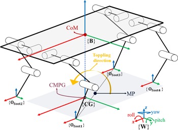
Since the expected displacement of the robot in the y direction is zero, and the virtual force in the y direction is precisely controlled, the displacement of the CoM in the y axis is almost zero. Therefore, when CMPG is before or behind MP in the X direction, two more situations are analyzed. One of the situations is shown in Fig. 4. When CMPG is in front of MP on the x axis, the gravity of CoM will cause the robot to topple around the line connecting diagonal supporting feet, i.e., the robot will rotate clockwise around the x and y axes. Therefore, virtual torques
 $^{\textrm{B}}{\textrm{}\textrm{T}}_{\textrm{C}\textrm{o}\textrm{M}\textrm{x}\textrm{}\textrm{}}$
and
 $^{\textrm{B}}{\textrm{}\textrm{T}}_{\textrm{C}\textrm{o}\textrm{M}\textrm{y}\textrm{}\textrm{}}$
should be counterclockwise. So
 \begin{align}\left[ {^{\textrm{B}}{{\textrm{F}}_{{\textrm{CoMy}}}}\,{\,^{\textrm{B}}}{{\textrm{F}}_{{\textrm{CoMz}}}}\,{\,^{\textrm{B}}}{{\textrm{T}}_{{\textrm{CoMx}}}}\,{\,^{\textrm{B}}}{{\textrm{T}}_{{\textrm{CoMy}}}}\,{\,^{\textrm{B}}}{{\textrm{T}}_{{\textrm{CoMz}}}}} \right] = {\textrm{[}}0\,\,{\textrm{Mg}}\, \lt \,0\, \lt \,0\,\,0]\end{align}
CMPG is in front of MP.

The relationship between foot positions in body coordinate is
 \begin{align} \left\{\begin{array}{c}{}_{\textrm{}}{}^{\textrm{B}}{\textrm{d}}_{\textrm{x}\textrm{i}} \lt -{}_{\textrm{}}{}^{\textrm{B}}{\textrm{d}}_{\textrm{x}\textrm{i}+2}\\ \\[-7pt] ^{\textrm{B}}{\textrm{d}}_{\textrm{y}\textrm{i}}=-{}_{\textrm{}}{}^{\textrm{B}}{\textrm{d}}_{\textrm{y}\textrm{i}+2}\\ \\[-7pt] ^{\textrm{B}}{\textrm{d}}_{\textrm{z}\textrm{i}}={}_{\textrm{}}{}^{\textrm{B}}{\textrm{d}}_{\textrm{z}\textrm{i}+2}\end{array}\right.\end{align}
Eq. (9) is applied to calculate the ground reaction forces, and x ground reaction forces are obtained:
 \begin{align} \left\{\begin{array}{l}{}_{\textrm{}}{}^{\textrm{W}}{\textrm{F}}_{\textrm{f}\textrm{x}\_{\bf{i}}\textrm{}\textrm{}}={}_{\textrm{}}{}^{\textrm{W}}{\textrm{F}}_{\textrm{f}\textrm{x}\_{\bf{i}}+2\textrm{}\textrm{}} \gt 0\\ \\[-7pt] ^{\textrm{B}}{\textrm{F}}_{\textrm{C}\textrm{o}\textrm{M}\textrm{x}\textrm{}\textrm{}}={}_{\textrm{}}{}^{\textrm{W}}{\textrm{F}}_{\textrm{f}\textrm{x}\_{\bf{i}}\textrm{}\textrm{}}+{}_{\textrm{}}{}^{\textrm{W}}{\textrm{F}}_{\textrm{f}\textrm{x}\_{\bf{i}}+2\textrm{}\textrm{}} \gt 0\end{array}\right.\end{align}
The result shows that the robot will generate positive locomotion on the x axis with a balanced body. Furthermore, the far CMPG is from MP, the fast the robot moves along the x positive axis.
MP is in front of CMPG.

Another situation is shown in Fig. 5. When MP is in front of CMPG on the x axis, the gravity of CoM will cause the robot to topple around the line connecting diagonal supporting feet, i.e., the robot will rotate counterclockwise around the x and y axes. Therefore, virtual torques
 $^{\textrm{B}}{\textrm{}\textrm{T}}_{\textrm{C}\textrm{o}\textrm{M}\textrm{x}\textrm{}\textrm{}}$
and
 $^{\textrm{B}}{\textrm{}\textrm{T}}_{\textrm{C}\textrm{o}\textrm{M}\textrm{y}\textrm{}\textrm{}}$
should be clockwise. So
 \begin{align}\left[ {^{\textrm{B}}{{\textrm{F}}_{{\textrm{CoMy}}}}\quad {\,^{\textrm{B}}}{{\textrm{F}}_{{\textrm{CoMz}}}}{\quad ^{\textrm{B}}}{{\textrm{T}}_{{\textrm{CoMx}}}}{\quad ^{\textrm{B}}}{{\textrm{T}}_{{\textrm{CoMy}}}}{\quad ^{\textrm{B}}}{{\textrm{T}}_{{\textrm{CoMz}}}}} \right] = \left[ {0\,\,{\textrm{Mg}} \gt 0 \gt 0\,\,0} \right]\end{align}
The relationship between foot positions in body coordinate is
 \begin{align} \left\{\begin{array}{c}{}_{\textrm{}}{}^{\textrm{B}}{\textrm{d}}_{\textrm{x}\textrm{i}} \gt -{}_{\textrm{}}{}^{\textrm{B}}{\textrm{d}}_{\textrm{x}\textrm{i}+2}\\ \\[-7pt] ^{\textrm{B}}{\textrm{d}}_{\textrm{y}\textrm{i}}=-{}_{\textrm{}}{}^{\textrm{B}}{\textrm{d}}_{\textrm{y}\textrm{i}+2}\\ \\[-7pt] ^{\textrm{B}}{\textrm{d}}_{\textrm{z}\textrm{i}}={}_{\textrm{}}{}^{\textrm{B}}{\textrm{d}}_{\textrm{z}\textrm{i}+2}\end{array}\right.\end{align}
Eq. (9) is applied to calculate the ground reaction forces, and x ground reaction force is obtained:
 \begin{align} \left\{\begin{array}{c}{}_{\textrm{}}{}^{\textrm{W}}{\textrm{F}}_{\textrm{f}\textrm{x}\_{\bf{i}}\textrm{}\textrm{}}={}_{\textrm{}}{}^{\textrm{W}}{\textrm{F}}_{\textrm{f}\textrm{x}\_{\bf{i}}+2\textrm{}\textrm{}} \lt 0\\ \\[-7pt] ^{\textrm{B}}{\textrm{F}}_{\textrm{C}\textrm{o}\textrm{M}\textrm{x}\textrm{}\textrm{}}={}_{\textrm{}}{}^{\textrm{W}}{\textrm{F}}_{\textrm{f}\textrm{x}\_{\bf{i}}\textrm{}\textrm{}}+{}_{\textrm{}}{}^{\textrm{W}}{\textrm{F}}_{\textrm{f}\textrm{x}\_{\bf{i}}+2\textrm{}\textrm{}} \lt 0\end{array}\right.\end{align}
The result shows that the robot will generate negative locomotion on the x axis with a balanced body. Furthermore, the far MP is from CMPG, the fast the robot moves along the x negative axis.
Although x virtual force can be changed by adjusting the position of CMPG with respect to MP, there is still a difference between passive x virtual force and required x virtual force. Fortunately, based on the changing trend of passive x virtual force, rough x velocity control can be achieved.
3.2. Selection of foot landing point
The relative position between CMPG and MP can change the passive x virtual force. The position adjustment can be executed before starting, getting an initial passive x virtual force. The velocity during locomotion can be adjusted by selecting the landing point of the swinging leg. As the theory proposed by Raibert, selections of the landing point of the swinging leg will change the forward velocity of the robot [Reference Raibert and Tello21]. The theory is implemented in this paper after reasonable modifications. A new form is proposed:
 \begin{align}^{\textrm{B}}{\textrm{X}}_{\textrm{f}\textrm{o}\textrm{o}\textrm{t}\textrm{T}\_{\bf{i}}}=\textrm{S}({}_{\textrm{}}{}^{\textrm{B}}{\textrm{V}}_{\textrm{X}\textrm{C}\textrm{o}\textrm{M}}{\boldsymbol\cdot} {\textrm{T}}_{\textrm{s}\textrm{t}\textrm{a}\textrm{n}\textrm{c}\textrm{e}}/2)\end{align}
where S is the distance regulating factor,
 $ {\textrm{T}}_{\textrm{s}\textrm{t}\textrm{a}\textrm{n}\textrm{c}\textrm{e}}$
is the stance period, and
 $^{\textrm{B}}{\textrm{X}}_{\textrm{f}\textrm{o}\textrm{o}\textrm{t}\textrm{T}\_{\bf{i}}}$
is the position of the landing point relative to BOfxi in Eq. (1).
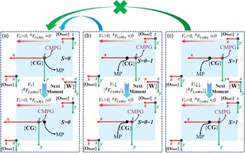
Assume that the robot moves along x axis with positive velocity. The analysis is carried out as shown in Fig. 6. If S equals 0 as shown in Fig. 6(a), the moment when legs status switch, i.e., stance leg becomes swing leg while swing leg becomes stance leg, CMPG overlaps MP, which indicates that the robot will move at the same speed until the next moment. Once CMPG surpasses MP, the robot will accelerate due to x positive virtual force. If S is within 0∼1 shown as Fig. 6(b), the moment when legs status switch, CMPG is behind MP, which indicates that the robot will slow down due to the x negative virtual force with decreasing x negative virtual force. After a while, CMPG will reach MP and become a situation as shown in Fig. 6(a). Furthermore, the robot is bound to move forward until the next switch of the legs before velocity reduces to zero. If S is greater than 1 as shown in Fig. 6(c), the moment when legs status switch, CMPG is far behind MP, so the robot will decelerate with a large x negative acceleration due to large x negative virtual force. However, CMPG will never reach MP to become a situation as shown in Fig. 6(a). The robot will fail to move forward to reach the next switch of the legs before velocity reduces to zero, and the locomotion of the robot will be converted into x negative direction. Therefore, the selection of landing point for the swing leg can adjust an average velocity of the robot.
A diagram about influence of S factor, where CMPG overlaps CoM.

3.3. Trajectory of foot of swing leg
This paper focuses on locomotion on flat ground without considering obstacles and irregular terrains. Therefore, the trajectories of the foot of the swinging leg in the x and z direction are generated by cubic interpolation, and the trajectory of the foot in the y direction is kept zero due to zero lateral displacement.
Trajectory of foot in x direction is as follows:
 \begin{align}^{\textrm{B}}{\textrm{X}}_{\textrm{f}\textrm{o}\textrm{o}\textrm{t}\_{\bf{i}}}\left(\textrm{t}\right)=\left\{\begin{array}{c@{\quad}l}-\dfrac{4{}_{\textrm{}}{}^{\textrm{W}}{\textrm{V}}_{\textrm{C}\textrm{o}\textrm{M}\textrm{x}0}}{{\textrm{T}}_{\textrm{f}\textrm{l}\textrm{y}}}{\textrm{t}}^{2}+{}_{\textrm{}}{}^{\textrm{W}}{\textrm{V}}_{\textrm{C}\textrm{o}\textrm{M}\textrm{x}0}t&0\le t \lt \dfrac{{\textrm{T}}_{\textrm{f}\textrm{l}\textrm{y}}}{4}\\ \\[-9pt] \dfrac{-4{\textrm{T}}_{\textrm{f}\textrm{l}\textrm{y}}{}_{\textrm{}}{}^{\textrm{W}}{\textrm{V}}_{\textrm{C}\textrm{o}\textrm{M}\textrm{x}0}-16{}_{\textrm{}}{}^{\textrm{B}}{\textrm{X}}_{\textrm{f}\textrm{o}\textrm{o}\textrm{t}\textrm{T}\_{\bf{i}}}}{{\textrm{T}}_{\textrm{f}\textrm{l}\textrm{y}}^{3}}{\textrm{t}}^{3}+\dfrac{7{\textrm{T}}_{\textrm{f}\textrm{l}\textrm{y}}{}_{\textrm{}}{}^{\textrm{W}}{\textrm{V}}_{\textrm{C}\textrm{o}\textrm{M}\textrm{x}0}-24{}_{\textrm{}}{}^{\textrm{B}}{\textrm{X}}_{\textrm{f}\textrm{o}\textrm{o}\textrm{t}\textrm{T}\_{\bf{i}}}\textrm{}}{{\textrm{T}}_{\textrm{f}\textrm{l}\textrm{y}}^{2}}{\textrm{t}}^{2}+&\\ \\[-9pt] \dfrac{-15{\textrm{T}}_{\textrm{f}\textrm{l}\textrm{y}}{}_{\textrm{}}{}^{\textrm{W}}{\textrm{V}}_{\textrm{C}\textrm{o}\textrm{M}\textrm{x}0}-36{}_{\textrm{}}{}^{\textrm{B}}{\textrm{X}}_{\textrm{f}\textrm{o}\textrm{o}\textrm{t}\textrm{T}\_{\bf{i}}}\textrm{}}{4{\textrm{T}}_{\textrm{f}\textrm{l}\textrm{y}}}t+\dfrac{9{\textrm{T}}_{\textrm{f}\textrm{l}\textrm{y}}{}_{\textrm{}}{}^{\textrm{W}}{\textrm{V}}_{\textrm{C}\textrm{o}\textrm{M}\textrm{x}0}+16{}_{\textrm{}}{}^{\textrm{B}}{\textrm{X}}_{\textrm{f}\textrm{o}\textrm{o}\textrm{t}\textrm{T}\_{\bf{i}}}\textrm{}}{16}\dfrac{{\textrm{T}}_{\textrm{f}\textrm{l}\textrm{y}}}{4}& \le t \lt \dfrac{{3\textrm{T}}_{\textrm{f}\textrm{l}\textrm{y}}}{4}\\ \\[-9pt] ^{\textrm{B}}{\textrm{X}}_{\textrm{f}\textrm{o}\textrm{o}\textrm{t}\textrm{T}\_{\bf{i}}}& t\ge \dfrac{{3\textrm{T}}_{\textrm{f}\textrm{l}\textrm{y}}}{4}\end{array}\right.\end{align}
where
 $ {\textrm{T}}_{\textrm{f}\textrm{l}\textrm{y}}$
is the swing period.
 $^{\textrm{W}}{\textrm{V}}_{\textrm{C}\textrm{o}\textrm{M}\textrm{x}0}$
is the velocity of CoM when foot status switches.
The position of the landing point in body coordinate is
 \begin{align}^{\textrm{B}}{\textrm{X}}_{\textrm{f}\textrm{o}\textrm{o}\textrm{t}\_{\bf{i}}}\left({\textrm{T}}_{\textrm{f}\textrm{l}\textrm{y}}\right)={}_{\textrm{}}{}^{\textrm{B}}{\textrm{X}}_{\textrm{f}\textrm{o}\textrm{o}\textrm{t}\textrm{T}\_{\bf{i}}}+{{}_{\textrm{}}{}^{\textrm{B}}\textrm{O}}_{\textrm{f}\textrm{x}\textrm{i}}\end{align}
Trajectory of foot in z direction is as follows:
 \begin{align} {\textrm{Z}}_{\textrm{f}\textrm{o}\textrm{o}\textrm{t}\_{\bf{i}}}\left(\textrm{t}\right)=\left\{\begin{array}{c@{\quad}l}\dfrac{16{}_{\textrm{}}{}^{\textrm{B}}{\textrm{Z}}_{\textrm{f}\textrm{o}\textrm{o}\textrm{t}0\_{\bf{i}}}-16{}_{\textrm{}}{}^{\textrm{B}}{\textrm{Z}}_{\textrm{f}\textrm{o}\textrm{o}\textrm{T}\textrm{t}\_{\bf{i}}}}{{\textrm{T}}_{\textrm{f}\textrm{l}\textrm{y}}^{3}}{\textrm{t}}^{2}+\dfrac{12{}_{\textrm{}}{}^{\textrm{B}}{\textrm{Z}}_{\textrm{f}\textrm{o}\textrm{o}\textrm{T}\textrm{t}\_{\bf{i}}}-12{}_{\textrm{}}{}^{\textrm{B}}{\textrm{Z}}_{\textrm{f}\textrm{o}\textrm{o}\textrm{t}0\_{\bf{i}}}}{{\textrm{T}}_{\textrm{f}\textrm{l}\textrm{y}}^{2}}+{}_{\textrm{}}{}^{\textrm{B}}{\textrm{Z}}_{\textrm{f}\textrm{o}\textrm{o}\textrm{t}0\_{\bf{i}}}&0\le t \lt \dfrac{{\textrm{T}}_{\textrm{f}\textrm{l}\textrm{y}}}{2}\\ \\[-7pt] \dfrac{4{}_{\textrm{}}{}^{\textrm{B}}{\textrm{Z}}_{\textrm{f}\textrm{o}\textrm{o}\textrm{t}0\_{\bf{i}}}-4{}_{\textrm{}}{}^{\textrm{B}}{\textrm{Z}}_{\textrm{f}\textrm{o}\textrm{o}\textrm{T}\textrm{t}\_{\bf{i}}}}{{\textrm{T}}_{\textrm{f}\textrm{l}\textrm{y}}^{2}}{\textrm{t}}^{2}+\dfrac{4{}_{\textrm{}}{}^{\textrm{B}}{\textrm{Z}}_{\textrm{f}\textrm{o}\textrm{o}\textrm{T}\textrm{t}\_{\bf{i}}}-4{}_{\textrm{}}{}^{\textrm{B}}{\textrm{Z}}_{\textrm{f}\textrm{o}\textrm{o}\textrm{t}0\_{\bf{i}}}}{{\textrm{T}}_{\textrm{f}\textrm{l}\textrm{y}}}+{}_{\textrm{}}{}^{\textrm{B}}{\textrm{Z}}_{\textrm{f}\textrm{o}\textrm{o}\textrm{t}0\_{\bf{i}}}&\dfrac{{\textrm{T}}_{\textrm{f}\textrm{l}\textrm{y}}}{2}\le t \lt Q{\textrm{T}}_{\textrm{f}\textrm{l}\textrm{y}}\\ \\[-7pt] ^{\textrm{B}}{\textrm{Z}}_{\textrm{f}\textrm{o}\textrm{o}\textrm{t}0\_{\bf{i}}}&t\ge Q{\textrm{T}}_{\textrm{f}\textrm{l}\textrm{y}}\end{array}\right.\end{align}
where
 $^{\textrm{B}}{\textrm{Z}}_{\textrm{f}\textrm{o}\textrm{o}\textrm{t}0\_{\bf{i}}}$
equals$
 $ {{}_{\textrm{}}{}^{\textrm{B}}\textrm{O}}_{\textrm{f}\textrm{z}\textrm{i}}$
.
 $^{\textrm{B}}{\textrm{Z}}_{\textrm{f}\textrm{o}\textrm{o}\textrm{t}0\_{\bf{i}}}$
is the z position of foot when foot status switches.
 $^{\textrm{B}}{\textrm{Z}}_{\textrm{f}\textrm{o}\textrm{o}\textrm{T}\textrm{t}\_{\bf{i}}}$
is the height which the swinging leg lifts. Q is time adjusting factor with range from 0.9∼1. The larger the Q is, the slower the landing time of the foot is, which brings less impulsive force to the foot.
VMC for foot of swing leg.

VMC is also implemented in foot shown as Fig. 7.
 \begin{align}\left\{ {\begin{array}{*{20}{c}}{{}_{{\;}}^{\textrm{B}}{{\textrm{F}}_{{\textrm{fvmcx}}\_{\textrm{i\;}}}} = \;{{\textrm{K}}_{{\textrm{pfx}}}}\!\left( {{}_{{\;}}^{\textrm{B}}{{\textrm{X}}_{{\textrm{foot}}\_{\textrm{i}}}}({\textrm{t}}) - {}_{{\;}}^{\textrm{B}}{{\textrm{X}}_{{\textrm{foot}}\_{\textrm{i}}}}} \right) + {{\textrm{B}}_{{\textrm{pfx}}}}\!\left(\dfrac{{{\textrm{d}}{}_{{\;}}^{\textrm{B}}{{\textrm{X}}_{{\textrm{foot}}\_{{\textrm{i}}_{{\;}}}}}({\textrm{t}})}}{{{\textrm{dt}}}} - \dfrac{{{\textrm{d}}{}_{{\;}}^{\textrm{B}}{{\textrm{X}}_{{\textrm{foot}}\_{{\textrm{i}}_{{\;}}}}}}}{{{\textrm{dt}}}}\right)}\\ \\[-7pt] {{}_{{\;}}^{\textrm{B}}{{\textrm{F}}_{{\textrm{fvmcy}}\_{\textrm{i\;}}}} = \;{{\textrm{K}}_{{\textrm{pfy}}}}\!\left( {{}_{{\;}}^{\textrm{B}}{{\textrm{Y}}_{{\textrm{foot}}\_{\textrm{i}}}}({\textrm{t}}) - {}_{{\;}}^{\textrm{B}}{{\textrm{Y}}_{{\textrm{foot}}\_{\textrm{i}}}}} \right) + {{\textrm{B}}_{{\textrm{pfy}}}}\!\left(\dfrac{{{\textrm{d}}{}_{{\;}}^{\textrm{B}}{{\textrm{Y}}_{{\textrm{foot}}\_{{\textrm{i}}_{{\;}}}}}({\textrm{t}})}}{{{\textrm{dt}}}} - \dfrac{{{\textrm{d}}{}_{{\;}}^{\textrm{B}}{{\textrm{Y}}_{{\textrm{foot}}\_{{\textrm{i}}_{{\;}}}}}}}{{{\textrm{dt}}}}\right)}\\ \\[-7pt] {{}_{{\;}}^{\textrm{B}}{{\textrm{F}}_{{\textrm{fvmcz}}\_{\textrm{i\;}}}} = \;{{\textrm{K}}_{{\textrm{pfz}}}}\!\left( {{}_{{\;}}^{\textrm{B}}{{\textrm{Z}}_{{\textrm{foot}}\_{\textrm{i}}}}({\textrm{t}}) - {}_{{\;}}^{\textrm{B}}{{\textrm{Z}}_{{\textrm{foot}}\_{\textrm{i}}}}} \right) + {{\textrm{B}}_{{\textrm{pfz}}}}\!\left(\dfrac{{{\textrm{d}}{}_{{\;}}^{\textrm{B}}{{\textrm{Z}}_{{\textrm{foot}}\_{{\textrm{i}}_{{\;}}}}}({\textrm{t}})}}{{{\textrm{dt}}}} - \dfrac{{{\textrm{d}}{}_{{\;}}^{\textrm{B}}{{\textrm{Z}}_{{\textrm{foot}}\_{{\textrm{i}}_{{\;}}}}}}}{{{\textrm{dt}}}}\right)}\end{array}} \right.\end{align}
where
 $^{\textrm{B}}{{\textrm{F}}_{{\textrm{fvmcx}}\_{\textrm{i}}}}$
,
 $^{\textrm{B}}{{\textrm{F}}_{{\textrm{fvmcy}}\_{\textrm{i}}}}$
, and
 $^{\textrm{B}}{{\textrm{F}}_{{\textrm{fvmcz}}\_{\textrm{i}}}}$
are virtual forces of foot of leg i.
 ${{\textrm{K}}_{{\textrm{***}}}}$
and
 ${{\textrm{B}}_{{\textrm{***}}}}$
are stiffness coefficient and damping coefficient, respectively.
 $^{\textrm{B}}{{\textrm{X}}_{{\textrm{foot}}\_{\textrm{i}}}}({\textrm{t}})$
and
 $^{\textrm{B}}{{\textrm{Z}}_{{\textrm{foot}}\_{\textrm{i}}}}({\textrm{t}})$
are position changes over time, and
 $^{\textrm{B}}{{\textrm{Y}}_{{\textrm{foot}}\_{\textrm{i}}}}({\textrm{t}})$
is set as zero.
 $^{\textrm{B}}{{\textrm{X}}_{{\textrm{foot}}\_{\textrm{i}}}}$
,
 $^{\textrm{B}}{{\textrm{Y}}_{{\textrm{foot}}\_{\textrm{i}}}}$
, and
 $^{\textrm{B}}{{\textrm{Z}}_{{\textrm{foot}}\_{\textrm{i}}}}$
are initial positions of foot when foot status switch.
Joint torques of swing legs can be calculated as
 \begin{align}{\boldsymbol\tau _{i}} = {}^{\bf{B}}{\bf{J}}_{\bf{i}}^{\bf{T}}{}^B{\bf{F}_{\bf{fvm}{{\bf{c}}_{\bf{i}}}}}\end{align}
where
 ${}^B{F_{fvmc\_i}} = {\left[ {{}_{{\;}}^{\textrm{B}}{{\textrm{F}}_{{\textrm{fvmcx}}\_{\textrm{i}}}}\;{}_{{\;}}^{\textrm{B}}{{\textrm{F}}_{{\textrm{fvmcy}}\_{\textrm{i}}}}\;{}_{{\;}}^{\textrm{B}}{{\textrm{F}}_{{\textrm{fvmcz}}\_{\textrm{i}}}}} \right]^{\textrm{T}}}$
.
3.4. Active intervention of passive control state
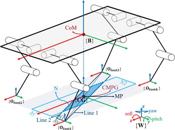
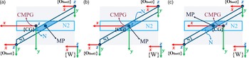
In order to compensate for the rough control of velocity mentioned above, the RIC is proposed in this paper. It is known that the robot keeps balanced when CMPG overlaps MP, i.e., lateral displacement will be zero even if y virtual force is set as passive control state. Based on the analysis, a tiny area around PM is planned for RIC. If CMPG is within the tiny area, y virtual force is set as passive control state, and x virtual force is accurately controlled to adjust x velocity, which only generates slight lateral displacement. The tiny area N is planned as Fig. 8, e.g., the N area here is associated with leg 1 and leg 3.
Tiny area for RIC.

N1 area is a parallelogram consisting of Line 1, Line 2, and Δy. Line 1 and Line 2 are represented as
 \begin{align}\left\{ {\begin{array}{*{20}{c}}{{}_{{\;}}^{\textrm{B}}{{\textrm{y}}_{{\textrm{l}}1}} = \;\dfrac{{{}_{{\;}}^{\textrm{B}}{{\textrm{d}}_{{\textrm{y}}3}} - {}_{{\;}}^{\textrm{B}}{{\textrm{d}}_{{\textrm{y}}1'}}}}{{{}_{{\;}}^{\textrm{B}}{{\textrm{d}}_{{\textrm{x}}3}} - {}_{{\;}}^{\textrm{B}}{{\textrm{d}}_{{\textrm{x}}1'}}}}\left( {{}_{{\;}}^{\textrm{B}}{{\textrm{x}}_{{\textrm{l}}1}} - {}_{{\;}}^{\textrm{B}}{{\textrm{d}}_{{\textrm{x}}1'}}} \right) + {}_{{\;}}^{\textrm{B}}{{\textrm{d}}_{{\textrm{y}}1'}}}\\ \\[-7pt] {{}_{{\;}}^{\textrm{B}}{{\textrm{y}}_{{\textrm{l}}2}} = \;\dfrac{{{}_{{\;}}^{\textrm{B}}{{\textrm{d}}_{{\textrm{y}}3'}} - {}_{{\;}}^{\textrm{B}}{{\textrm{d}}_{{\textrm{y}}{1^{{\;}}}}}}}{{{}_{{\;}}^{\textrm{B}}{{\textrm{d}}_{{\textrm{x}}3'}} - {}_{{\;}}^{\textrm{B}}{{\textrm{d}}_{{\textrm{x}}{1^{{\;}}}}}}}\left( {{}_{{\;}}^{\textrm{B}}{{\textrm{x}}_{{\textrm{l}}2}} - {}_{{\;}}^{\textrm{B}}{{\textrm{d}}_{{\textrm{x}}{1^{{\;}}}}}} \right) + {}_{{\;}}^{\textrm{B}}{{\textrm{d}}_{{\textrm{y}}{1^{{\;}}}}}}\end{array}} \right.\end{align}
where
 $^{\textrm{B}}{{\textrm{d}}_{{\textrm{y}}3}} + \Delta {\textrm{y}} = {{\;}}{}_{{\;}}^{\textrm{B}}{{\textrm{d}}_{{\textrm{y}}3'}}$
,
 $^{\textrm{B}}{{\textrm{d}}_{{\textrm{y}}1'}} + \Delta {\textrm{y}} = {{\;}}{}_{{\;}}^{\textrm{B}}{{\textrm{d}}_{{\textrm{y}}{1^{{\;}}}}}$
.
N2 area is a rectangle that can be defined as {
 $^{\textrm{B}}{{\textrm{d}}_{{\textrm{x}}{1^{{\;}}}}} \lt x \lt {}_{{\;}}^{\textrm{B}}{{\textrm{d}}_{{\textrm{x}}{3^{{\;}}}}}$
∩
 $ - \Delta y' \lt y \lt \Delta y'$
}.
N area is the intersection of N1 and N2. If CMPG is contained inside N area, x virtual force is contained in the control list and y virtual force is set as passive control state. Virtual forces and torques are
 \begin{align}{}^{\bf{B}}{{\bf{F}}_{{\bf{CoM}}}} = {{}}{\left[ {\;{}_{{\;}}^{\textrm{B}}{{\textrm{F}}_{{\textrm{CoMx}}}}\;{0_{{{}}}}\;{}_{{\;}}^{\textrm{B}}{{\textrm{F}}_{{\textrm{CoMz}}}}{{\;}}{}_{{\;}}^{\textrm{B}}{{\;}}{{\textrm{T}}_{{\textrm{CoMx}}}}{}_{{\;}}^{\textrm{B}}{{\;}}{{\textrm{T}}_{{\textrm{CoMy}}}}{}_{{\;}}^{\textrm{B}}{{\;}}{{\textrm{T}}_{{\textrm{CoMz}}}}} \right]^T}\end{align}
Eq. (19) and Eq. (22) are amended for the analysis of passive y virtual force:
 \begin{align}\left\{ {\begin{array}{*{20}{c}}{\;{}_{{\;}}^{\textrm{B}}{{\textrm{d}}_{{\textrm{xi}}}} = \; - {}_{{\;}}^{\textrm{B}}{{\textrm{d}}_{{\textrm{xi}} + 2}}}\\ \\[-7pt] {{}_{{\;}}^{\textrm{B}}{{\textrm{d}}_{{\textrm{yi}}}}\;( \gt or \lt )\; - {}_{{\;}}^{\textrm{B}}{{\textrm{d}}_{{\textrm{yi}} + 2}}}\\ \\[-7pt] {{}_{{\;}}^{\textrm{B}}{{\textrm{d}}_{{\textrm{zi}}}} = \;{}_{{\;}}^{\textrm{B}}{{\textrm{d}}_{{\textrm{zi}} + 2}}}\end{array}} \right.\end{align}
The size of the N area determines the degree of control of x virtual force. The larger the N area is, the stronger the intervention is, causing more accurate x velocity but larger lateral displacement. The attitude of the robot keeps balanced under the different sizes of the N area.
Fig. 9 is a detailed diagram showing the working theory of the N area intervention. In Fig. 9(a), x virtual force is passive control, which causes the robot to accelerate forward. In Fig. 9(b), x virtual force is actively controlled to adjust velocity, and y virtual force is set as passive control, bringing tiny lateral displacement. In Fig. 9(c), passive control of x virtual force results in acceleration at the x negative axis.
Top view of the robot about the relationship between CMPG and N area, where CMPG overlaps CoM. (a) CMPG is outside and before N area. (b) CMPG is inside N area. (c) CMPG is outside and behind N area.

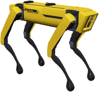
Spotmini model in Webots.

4. Verification Simulation
4.1. Parameter setting
Simulation is conducted based on open source software Webots, with the free model Spotmini provided by Webots shown in Fig. 10. Some parameters are changed, including model size, mass, maximum motor torque, maximum motor speed, and position of CoM.
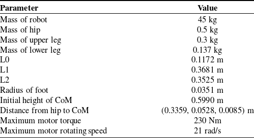
Parameters of the robot.

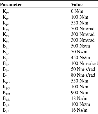
Parameters of K and D.

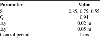
Table I demonstrates that the total mass of legs accounts for only eight percent of the robot mass, which accords with the requirements of the method proposed in this paper. CoM is located at the center of four hip joints. Table II shows all the stiffness coefficients and damping coefficients of the controller. S in Table III is used for adjusting the landing point, and the value decreases along with the decreasing speed. Δy and Δy’ are related to the N area.
As mentioned before, this research focuses on the balance control when the robot moves in the x axis in trot gait, so x virtual force is set as a passive control state in most of the period except for RIC, ensuring body balanced. The average locomotive speed is set to 0.5 m/s since the quadruped robot moves at a low speed to keep highly balanced for some critical tasks including transporting precious goods, mapping with radars or cameras, and so on. In order to quickly start the robot, CMPG is 0.03 m ahead of MP initially. The operating period of the legs is 1 s.
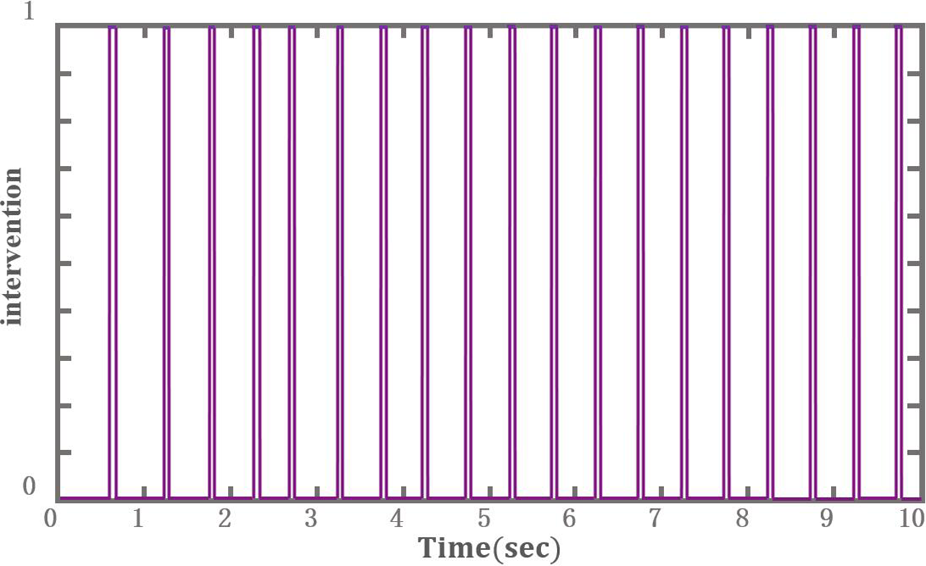
Adjusting intervention of x virtual force. 0 and 1 are without and with intervention, respectively.

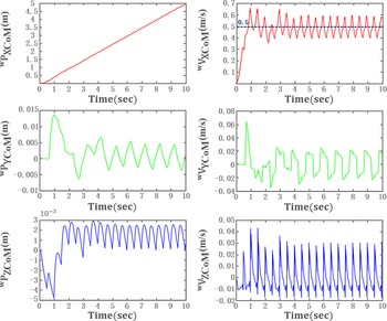
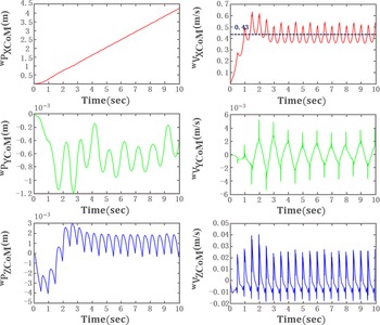
Variation of displacements and velocities of CoM along with time with intervention.

4.2. Motion simulation of the robot with intervention
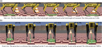
Figure 11 shows that twice interventions are applied within a period except for the first period. Because of the relative position between CMPG and MP at the beginning, intervention in the first half period fails to activate. When the robot enters the stable condition, intervention happens when CMPG is within the N area.
Parameters of adjusting factors.

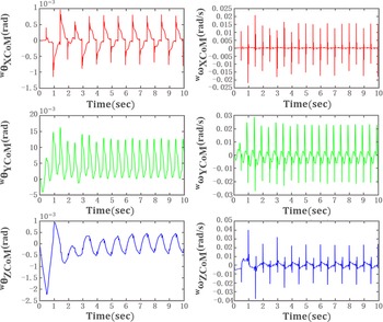
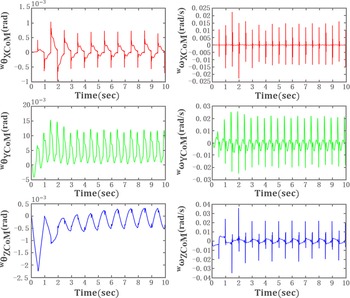
Variation of angles and angular speed of the robot along with time with intervention.

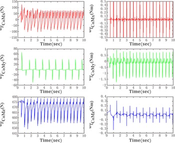
Figures 12 and 13 demonstrate the variation of 12 states of the robot with the intervention. All status of the robot fluctuate significantly at the beginning due to intrinsic inertial force, but only the steady condition is studied. Figure 12 shows that an average speed in the x axis is 0.5 m/s, with a fluctuating range within 0.19 m/s. The lateral displacement is from −0.004 m to 0.005 m for the reason that y virtual force is set as passive control during the intervention. The displacement fluctuation in the z axis is less than 0.003 m, with the velocity fluctuating range less than 0.05 m/s. Meanwhile, as shown in Fig. 13, the fluctuating range of angles around the x, y, and z axes are less than 0.0036 rad, 0.0013 rad, and 0.001 rad, respectively. The fluctuating ranges of angular velocities are less than 0.035 rad/s, 0.045 rad/s, and 0.047 rad/s, respectively. The change rules of virtual forces and torques completely match the 12 states. As shown in Fig. 14, the fluctuating range of x and y virtual forces are less than 200 N and 80 N, respectively, with the fluctuating range of z virtual force within 30 N.
Variation of visual forces and torques along with time with intervention.

Therefore, the intervention that occurs twice a period effectively adjusts x velocity by allowing a tiny lateral displacement. Furthermore, the operation that sets x virtual force as passive control state ensures considerably balanced control of the rest DoFs of the robot.
4.3. Motion simulation of the robot without intervention
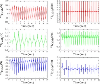
Figures 15 and 16 demonstrate the variation of twelve states of the robot without intervention. Figure 15 shows that an average speed in the x axis is 0.43 m/s, with the fluctuating range within 0.2 m/s. The fluctuating range of lateral displacement is within 0.0012 m without intervention. The displacement in the z axis is less than 0.003 m, with velocity fluctuating range less than 0.05 m/s. Meanwhile, as shown in Fig. 16, the fluctuating ranges of angles around the x, y, and z axes are less than 0.002 rad, 0.0013 rad, and 0.0009 rad, respectively. The fluctuating ranges of angular velocities are less than 0.03 rad/s, 0.043 rad/s, and 0.045 rad/s, respectively. As shown in Fig. 17, the change rules of virtual forces and torques completely match the twelve states. The fluctuating range of x and y virtual forces is less than 200 N and 0.6 N, respectively, with fluctuating range of z virtual force within 30 N.
Variation of displacements and velocities of CoM along with time without intervention.

Variation of angles and angular speed of the robot along with time without intervention.

Variation of visual forces and torques along with time without intervention.

Therefore, the balance control without intervention can guarantee that the robot is under the most balanced status. However, the difference between actual x velocity and desired x velocity is distinct.
4.4. Precision evaluation
According to the data in Figs. 12–17, the six-dimensional mechanical decoupling algorithm proposed in this paper achieves the excellent balance control of quadruped robots during trot. Without RIC, the attitude changes are extremely small, and the changes of height and lateral displacement are millimeter level. The average locomotive velocity approaches the expected value but fails to reach it. After RIC is implemented, the variations of attitude and height are still tiny. The maximum lateral displacement increases from 0.0012 m to 0.005 m, and the average locomotive velocity achieves the expected velocity of 0.5 m/s. The result indicates that the tiny sacrifice of accurate control of lateral displacement effectively enhances the accurate control of the average locomotive velocity. Moreover, the evaluation of control accuracy of the whole quadruped robot is required to carry out.
Since the rotations around three axes and height are precisely controlled, the variations of the average locomotive velocity and the maximum lateral displacement with and without RIC are the critical evaluating parameters. The evaluation function is utilized:
 \begin{align}{\textrm{E}} = 1 - \frac{{\sqrt {{{\left( {{}_{{\;}}^{\textrm{W}}{{\textrm{V}}_{{\textrm{XCoM}}\_{\textrm{ave}}}} - {}_{{\;}}^{\textrm{W}}{{\textrm{V}}_{{\textrm{XCoM}}\_{\textrm{exp}}}}} \right)}^2} + {{\left( {{}_{{\;}}^{\textrm{W}}{{\textrm{P}}_{{\textrm{YCoM}}\_{\textrm{max}}}} - {}_{{\;}}^{\textrm{W}}{{\textrm{P}}_{{\textrm{YCoM}}\_{\textrm{exp}}}}} \right)}^2}} }}{{\sqrt {\left| {{}_{{\;}}^{\textrm{W}}{{\textrm{V}}_{{\textrm{XCoM}}\_{\textrm{exp}}}}} \right| + \left| {{}_{{\;}}^{\textrm{W}}{{\textrm{P}}_{{\textrm{YCoM}}\_{\textrm{exp}}}}} \right|} }}\end{align}
where E is the evaluating index between 0 and 1, the larger the E is, the higher the accuracy is.
 $^{\textrm{W}}{{\textrm{V}}_{{\textrm{XCoM}}\_{\textrm{ave}}}}$
and
 $^{\textrm{W}}{{\textrm{V}}_{{\textrm{XCoM}}\_{\textrm{exp}}}}$
are the practical average and expected average locomotive velocity, respectively.
 $^{\textrm{W}}{{\textrm{P}}_{{\textrm{YCoM}}\_{\textrm{max}}}}$
and
 $^{\textrm{W}}{{\textrm{P}}_{{\textrm{YCoM}}\_{\textrm{exp}}}}$
are the maximum and expected lateral displacement, respectively.
 $\left| * \right|$
is the absolute value.
As mentioned above,
 $^{\textrm{W}}{{\textrm{V}}_{{\textrm{XCoM}}\_{\textrm{exp}}}}$
and
 $^{\textrm{W}}{{\textrm{P}}_{{\textrm{YCoM}}\_{\textrm{exp}}}}$
are 0.5 m/s and 0, respectively.
 $^{\textrm{W}}{{\textrm{V}}_{{\textrm{XCoM}}\_{\textrm{ave}}}}$
are 0.5 m/s and 0.43 m/s with and without RIC.
 $^{\textrm{W}}{{\textrm{P}}_{{\textrm{YCoM}}\_{\textrm{max}}}}$
are 0.005 m and 0.0012 m with and without RIC. After calculation, E are 0.9929 and 0.9010 with and without RIC. The result shows that the whole accuracy is increased distinctly with RIC.
4.5. Snapshots at critical moments
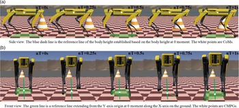
Snapshots of quadruped robot at every 0.25 s in steady moving status are demonstrated in Figs. 18 and 19. The robot body is maintained in super balance based on the method proposed in the paper. Moreover, no distinct fluctuations can be observed in the pictures, which further verifies that the method is available. In addition, at moments of 0.25 s and 0.75 s, CMPG is within the N area shown as the green area in Fig. 18, which means that the intervention is activated to adjust x velocity.
Snapshots of quadruped robot while moving in X axis with intervention. (a) Side view: the blue dash line is the reference line of the body height established based on the body height at 0 moment. The white points are CoMs. (b) Front view: the green line is a reference line extending from the Y-axis origin at 0 moment along the X-axis on the ground. The white points are CMPGs.

Snapshots of quadruped robot while moving in x axis without intervention. (a) Side view: the blue dash line is the reference line of the body height established based on the body height at 0 moment. The white points are CoMs. (b) Front view: the green line is a reference line extending from the Y-axis origin at 0 moment along the X-axis on the ground. The white points are CMPGs.

5. Conclusion
This paper proposes six-dimensional spatial mechanics decoupling algorithm to address balance control when the quadruped robot moves in trot gait. Compared to the current complex algorithm applied to the quadruped robot, the method proposed simplifies the calculating process, which only contains a 6 × 6 matrix inverse, cubic product, and other simple mathematic operations without any iteration calculations. By establishing of the matrix, which connects virtual forces and torques of CoM to ground reaction forces of the supporting legs, body balance control during trot gait is achieved after setting a passive control state. The trajectory of the foot of the swing leg is generated by cubic interpolation, and the landing point of the foot is selected to adjust the moving speed. Moreover, the intervention area is planned for compensating the adjustment of moving speed without influencing the balance of the body. Simulation results show that the quadruped robot has achieved balance during trot gait. The average speed of the robot is the same as desired speed when the intervention of x virtual force is implemented.
6. Discussion
This paper mainly focuses on the body balanced control while trotting by simplifying the calculation process, neglecting the accurate real-time speed control. The method proposed provides a new available strategy for the quadruped robot in balance control. What is more, the method proposed can be applied to other gaits by modifying some parameters in the 6 × 6 matrix. Further work should be done to accurately adjust moving speed without influencing balance.
Acknowledgments
The author is grateful to the predecessors who have made great efforts in the research of quadruped robot. The author also thanks Xiaoxiao Wen in South China University of Technology, Kun Wang in Zhejiang University, and Tianhai Wang in China Agricultural University for their friendly help. The author declares that there is no conflict of interest.