1 Introduction
As the Arctic region may become a possible shipping route (Smith & Stephenson Reference Smith and Stephenson2013), there has been an increasing interest in understanding the behaviour of a ship or other structure in water covered by an ice sheet over a large extent. The motion of a ship in such an environment is expected to be very different from that of a ship in the open sea. One of the main reasons is that the geophysical condition in the Arctic is different, or the typical wave which the ship encounters is different. Another reason is that when the ship is set into motion by an incoming wave, its radiated wave will be reflected by the ice sheet. It will propagate back to the ship and have further interactions with the ship. This makes interactions of a ship with the external environment more complex.
The work on wave/ice interactions without a floating body in the context of geophysics started very early. Following the work of Greenhill (Reference Greenhill1887), when the horizontal dimension of the ice sheet is much larger than its vertical dimension, it is very common to use the elastic plate model for the sea ice. In many cases, the fluid flow due to wave/ice interaction can be modelled by the linear velocity potential theory. These assumptions are valid for a wide range of problems in the polar region, as explained in the review papers by Squire et al. (Reference Squire, Dugan, Wadhams, Rottier and Liu1995) and Squire (Reference Squire2007, Reference Squire2011). Based on this model, Fox & Squire (Reference Fox and Squire1990) considered the problem of wave propagating from open sea to the shore fast ice. They obtained the reflection and transmission coefficients for a wave into a semi-infinite ice sheet. The wave direction was normal to the edge of ice sheet, and the problem was two-dimensional and was solved through matched eigenfunction expansions (MEE), in which the unknowns were found by numerically minimizing the errors in the matching conditions and edge conditions. This was then extended to the oblique incident wave by Fox & Squire (Reference Fox and Squire1994). A similar problem was considered by Sahoo, Yip & Chwang (Reference Sahoo, Yip and Chwang2001), where the unknowns in the eigenfunction expansions were found through introducing an inner product of orthogonality. The problem was also solved through the Wiener–Hopf method initiated by Evans & Davies (Reference Evans and Davies1968), as done by Balmforth & Craster (Reference Balmforth and Craster1999), Chung & Fox (Reference Chung and Fox2002) and Tkacheva (Reference Tkacheva2004). For an ice sheet of finite length or an ice floe, Meylan & Squire (Reference Meylan and Squire1993) obtained an approximate solution based on the large length assumption. They provided an explicit equation which showed that there would be an infinite number of discrete frequencies at which the reflection coefficient would be zero or perfect transmission would occur. The problem was also solved without the large length assumption by Meylan & Squire (Reference Meylan and Squire1994) through the Green function method. Chung & Linton (Reference Chung and Linton2005) considered an open lead or polynya, while Williams & Squire (Reference Williams and Squire2006) considered the case in which the surface of polynya was refrozen. Zero reflection was also found in these cases. For an infinite ice sheet with a crack, Barrett & Squire (Reference Barrett and Squire1996) solved the wave reflection problem of finite depth through an MEE method similar to that in Fox & Squire (Reference Fox and Squire1994). For infinite water depth, by using the Green function for the ice sheet without crack, Squire & Dixon (Reference Squire and Dixon2000) solved the problem for the normal incident wave, while Williams & Squire (Reference Williams and Squire2002) did the same for the oblique incident wave. By separating the problem into the symmetric and antisymmetric parts, Evans & Porter (Reference Evans and Porter2003) obtained the solution for an oblique wave in a series form for finite water depth, and localized edge waves travelling along the crack were found to be possible. The problem was further extended to the multiple parallel cracks of infinite length by Porter & Evans (Reference Porter and Evans2006), and to cracks of finite length by Porter & Evans (Reference Porter and Evans2007).
The work with the body present in the wave/ice interaction problem started relatively later. Das & Mandal (Reference Das and Mandal2006) used the multipole expansion method for wave scattering by a circular cylinder submerged below a surface entirely covered by an ice sheet. Wave reflection and transmission coefficients were obtained for various ice flexural stiffnesses. Sturova (Reference Sturova2014b ) obtained the Green function for the water surface covered by a semi-infinite ice sheet through the MEE method. The unknown coefficients were found through a matrix equation which was resolved for different source positions. The wave radiation problem by a submerged cylinder was solved through the boundary element method. This was further extended to the problem for infinitely extended ice sheet with a crack (Sturova Reference Sturova2015a ), and an ice floe or a polynya (Sturova Reference Sturova2015b ). The effect of an ice floe on the hydrodynamic coefficients of a submerged body was also considered by Tkacheva (Reference Tkacheva2015), in which the Green function was obtained through the Wiener–Hopf technique. For a body floating on a polynya, Ren, Wu & Thomas (Reference Ren, Wu and Thomas2016) solved the problem for a rectangular body using the MEE method, while Li, Shi & Wu (Reference Li, Shi and Wu2018) used a hybrid eigenfunction expansion and boundary element method and solved the problem for a floating body of arbitrary shape. Using the wide polynya approximation, Li, Shi & Wu (Reference Li, Shi and Wu2017a ) solved the problem of a body floating on polynya based on the solutions for polynya without a body and a floating body without ice. Explicit equations were derived, which uncovered the mechanism for the oscillatory behaviours of the hydrodynamic force and the body motion. The nonlinear effect of the body position during its motion was considered by Li, Shi & Wu (Reference Li, Shi and Wu2017b ) through using the multipole expansion for a circular cylinder.
In this paper, we consider the problem of wave interaction with a circular cylinder submerged in water covered by an ice sheet with a crack. Although the problem is two-dimensional (2-D), as in common in other physical problem, such a simplification is appropriate when the variation of the physical parameters in the third dimension is much smaller than that in the other two. Also the obtained results often shed some important insights into general three-dimensional problems. For this reason, the 2-D problem has been considered widely in the context of wave/ice interaction (Squire Reference Squire2007). For the problems in naval architecture, the 2-D solution for each cross-section of a ship can be incorporated into the strip method (Newman Reference Newman1977) and the so-called 2-D+t method (Faltinsen Reference Faltinsen2005) used as a practical design tool.
There are some significantly different features between the present work and those done previously. Firstly, we shall derive the Green function, or the potential due to a single source, which satisfies both the ice sheet and crack condition. This allows us to obtain the solution for wave diffraction by the ice crack directly, while this problem was solved by Evans & Porter (Reference Evans and Porter2003) using the Green function for the ice sheet without a crack. We shall show that our result is identical to theirs for this particular case. Secondly, we should mention that the Green function which satisfies both the ice sheet and crack condition was obtained by Sturova (Reference Sturova2015a ). She started the solution from the Green function without the crack. To satisfy the condition at the crack, expansions of the potential based on MEE were used on both sides of the crack. The series was then truncated at a finite number. The coefficients in the expansions were found through the solution of the matrix equation obtained from matching conditions at the interface. This is different from the free surface problem where the coefficients are given explicitly. The procedure was repeated for each different location of the source whose horizontal coordinate should not be the same as that of the crack. Here we shall use Fourier transform and the Green function is obtained in a simple integral form, which does not require re-derivation when the source is at a different point. Also infinite water depth is merely a special case of the present formation, for which the MEE is no longer applicable. It should be emphasized that the integral form of the Green function may be standard for a homogenous upper surface condition, as in Evans & Porter (Reference Evans and Porter2003) for an infinite ice sheet without a crack. However its derivation for the ice sheet with a crack is less straightforward and therefore it is one of the principal contributions of the present paper. Thirdly, in addition to being used more efficiently than the series form of Sturova (Reference Sturova2015a ) in the boundary element method for a body of arbitrary shape, from the derived Green function, we may obtain the potential due to multipoles through direct differentiation with respect to the position of the source. The method was initiated by Ursell (Reference Ursell1949, Reference Ursell1950) to solve the water wave interaction problem with a floating semi-circular cylinder and a submerged circular cylinder. His pioneering work had a major impact in naval architecture, especially in the development of strip theory for ship motion in waves. However, the equivalent multipole expansion method has not been developed in the problem of an ice sheet with a crack. Some attempts were made to use the multipole expansion method for a circular cylinder near the edge of a semi-infinite sheet (Sturova Reference Sturova2014a ). However, the coefficients in the series expansion for each multipole were obtained separately. Here by taking the advantage of the simple form of the newly derived Green function, the multipole is constructed directly through differentiation of the Green function with respect to the source position. Finally, a wide spacing approximation method (Srokosz & Evans Reference Srokosz and Evans1979) is adopted for this type of problem. This enables us to obtain accurate results from the solution for a cylinder without the crack and the solution for a crack without the cylinder, similar to that for a body in a wide polynya (Li et al. Reference Li, Shi and Wu2017a ). It also enables us to have some deep understanding of physical nature of the problem.
The paper is organized as follows. A description of the linearized velocity potential problem for the ice sheet with a crack is presented in § 2. The Green function, or the potential due to an oscillating source, is derived in § 3.1, from which the multipole expansion is constructed in § 3.2. The potentials for the radiation and diffraction problems of a submerged circular cylinder are then constructed in §§ 3.3 and 3.4 respectively. Special cases including the wide spacing approximation and deep water limit are considered in § 3.5. Results are presented and discussed in § 4, followed by the conclusion in § 5. In appendices A and B, the far field formulas for damping coefficient and wave exciting force are presented respectively, while in appendix C the Haskind relation for the wave exciting force is derived.
2 Mathematical model
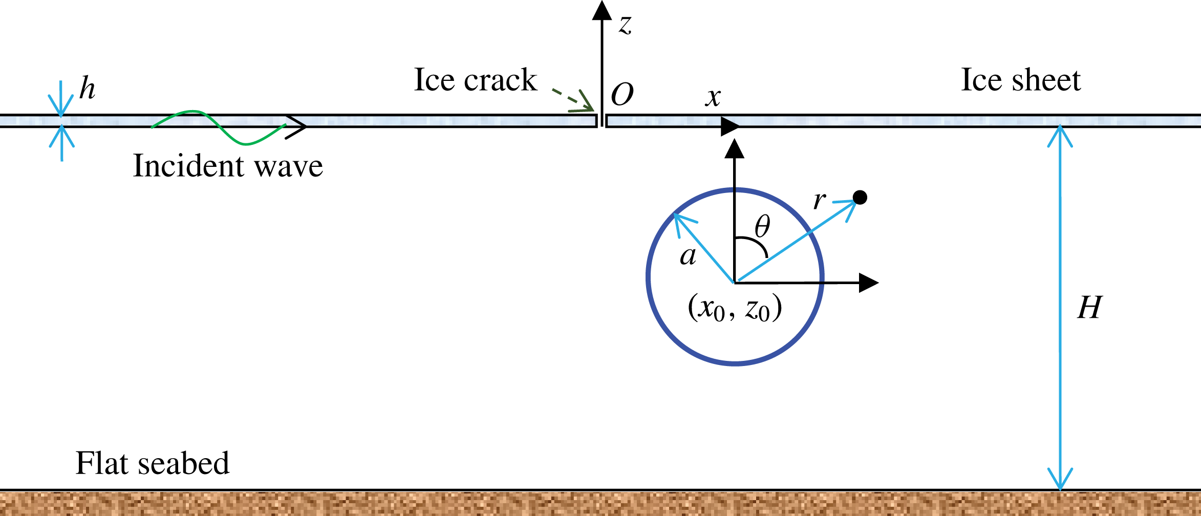
We consider the problem of wave interaction with a circular cylinder of radius
 $a$
submerged in water covered by an ice sheet with a crack, as sketched in figure 1. A Cartesian coordinate system
 $O{-}xz$
is defined, with the
 $x$
-axis along the undisturbed mean upper surface, and the
 $z$
-axis pointing vertically upwards. The ice sheet with uniform properties is extended from
 $x=-\infty$
to
 $x=+\infty$
. Its draught is assumed to be zero, and the crack is assumed to be located at
 $x=0$
, as shown in the figure.
Coordinate system and sketch of the problem.

The fluid with density
 $\unicode[STIX]{x1D70C}$
and depth
 $H$
is assumed to be inviscid, incompressible and homogeneous, and its motion to be irrotational. Thus the velocity potential
 $\unicode[STIX]{x1D6F7}$
can be introduced to describe the fluid flow. Under the assumption that the amplitude of the wave motion is small compared to its length and the dimension of the body, the linearized velocity potential theory can be further used. Based on the assumption that the motion is sinusoidal in time with frequency
 $\unicode[STIX]{x1D714}$
, the total velocity potential can be written in the following form
 $$\begin{eqnarray}\unicode[STIX]{x1D6F7}(x,z,t)=\text{Re}\left[\unicode[STIX]{x1D6FC}_{0}\unicode[STIX]{x1D719}_{0}(x,z)\text{e}^{\text{i}\unicode[STIX]{x1D714}t}+\mathop{\sum }_{j=1}^{2}\text{i}\unicode[STIX]{x1D714}\unicode[STIX]{x1D6FC}_{j}\unicode[STIX]{x1D719}_{j}(x,z)\text{e}^{\text{i}\unicode[STIX]{x1D714}t}\right],\end{eqnarray}$$
where the scattering potential
 $\unicode[STIX]{x1D719}_{0}$
contains the incident potential
 $\unicode[STIX]{x1D719}_{I}$
and diffracted potential
 $\unicode[STIX]{x1D719}_{D}$
,
 $\unicode[STIX]{x1D6FC}_{0}$
is the amplitude of the incident wave;
 $\unicode[STIX]{x1D719}_{j}$
 $(j=1,2)$
is the radiation potential due to body oscillation with complex amplitude
 $\unicode[STIX]{x1D6FC}_{j}$
in the
 $x$
and
 $z$
directions respectively. The rotational mode is not included in (2.1) as the rotation of a circular cylinder about its centre does not disturb the fluid. Mass conservation requires that the potential
 $\unicode[STIX]{x1D719}_{j}$
satisfies the Laplace’s equation
 $$\begin{eqnarray}\unicode[STIX]{x1D6FB}^{2}\unicode[STIX]{x1D719}_{j}=0,\quad (j=0,1,2),\end{eqnarray}$$
throughout the fluid. The ice sheet is modelled as a continuous elastic plate with uniform properties, i.e. thickness
 $h$
, density
 $\unicode[STIX]{x1D70C}_{0}$
, Young’s modulus
 $E$
, Poisson’s ratio
 $\unicode[STIX]{x1D708}$
are all constant. Thus the boundary condition on the ice sheet can be written as (Fox & Squire Reference Fox and Squire1990)
 $$\begin{eqnarray}\left(L\frac{\unicode[STIX]{x2202}^{4}}{\unicode[STIX]{x2202}x^{4}}-m\unicode[STIX]{x1D714}^{2}+\unicode[STIX]{x1D70C}g\right)\frac{\unicode[STIX]{x2202}\unicode[STIX]{x1D719}_{j}}{\unicode[STIX]{x2202}z}-\unicode[STIX]{x1D70C}\unicode[STIX]{x1D714}^{2}\unicode[STIX]{x1D719}_{j}=0,\quad (|x|>0,z=0),\end{eqnarray}$$
where
 $L=Eh^{3}/[12(1-\unicode[STIX]{x1D708}^{2})]$
is the effective flexural rigidity of the ice sheet, and
 $m=h\unicode[STIX]{x1D70C}_{0}$
is its mass per unit area. As the ice sheet has a crack at
 $x=0$
, zero bending moment and shear force are assumed there (Squire Reference Squire2007). This leads to the following two conditions
 $$\begin{eqnarray}\frac{\unicode[STIX]{x2202}^{2}}{\unicode[STIX]{x2202}x^{2}}\left(\frac{\unicode[STIX]{x2202}\unicode[STIX]{x1D719}_{j}}{\unicode[STIX]{x2202}z}\right)=0\quad \text{and}\quad \frac{\unicode[STIX]{x2202}^{3}}{\unicode[STIX]{x2202}x^{3}}\left(\frac{\unicode[STIX]{x2202}\unicode[STIX]{x1D719}_{j}}{\unicode[STIX]{x2202}z}\right)=0,\quad (x=0,z=0).\end{eqnarray}$$
It may be noticed that we can also impose other conditions at the crack, e.g. the two semi-infinite sheets are hinged or connected by springs. These can be done through specifying proper combinations of the displacements, slopes, bending moments and shear forces, on both sides of the crack. The impermeable condition on the body surface is
 $$\begin{eqnarray}\frac{\unicode[STIX]{x2202}\unicode[STIX]{x1D719}_{0}}{\unicode[STIX]{x2202}n}=0\quad \text{and}\quad \frac{\unicode[STIX]{x2202}\unicode[STIX]{x1D719}_{j}}{\unicode[STIX]{x2202}n}=n_{j},\quad (j=1,2),\end{eqnarray}$$
where
 $n_{1}$
and
 $n_{2}$
are the
 $x$
,
 $z$
components of the unit normal vector
 $\boldsymbol{n}$
pointing into the body. On the flat seabed, the following condition should be also enforced
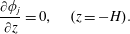 $$\begin{eqnarray}\frac{\unicode[STIX]{x2202}\unicode[STIX]{x1D719}_{j}}{\unicode[STIX]{x2202}z}=0,\quad (z=-H).\end{eqnarray}$$
The radiation condition at infinity requires the wave to propagate outwards
 $$\begin{eqnarray}\lim _{x\rightarrow \pm \infty }\left(\frac{\unicode[STIX]{x2202}\unicode[STIX]{x1D719}_{D}}{\unicode[STIX]{x2202}x}\pm \text{i}\unicode[STIX]{x1D706}\unicode[STIX]{x1D719}_{D}\right)=0\quad \text{and}\quad \lim _{x\rightarrow \pm \infty }\left(\frac{\unicode[STIX]{x2202}\unicode[STIX]{x1D719}_{j}}{\unicode[STIX]{x2202}x}\pm \text{i}\unicode[STIX]{x1D706}\unicode[STIX]{x1D719}_{j}\right)=0,\quad (j=1,2),\end{eqnarray}$$
where
 $\unicode[STIX]{x1D706}$
is the purely positive real root of the dispersion equation for a flexural gravity wave in the ice sheet, or
 $$\begin{eqnarray}K(\unicode[STIX]{x1D714},\unicode[STIX]{x1D706})\equiv (L\unicode[STIX]{x1D706}^{4}+\unicode[STIX]{x1D70C}g-m\unicode[STIX]{x1D714}^{2})\unicode[STIX]{x1D706}\tanh (\unicode[STIX]{x1D706}H)-\unicode[STIX]{x1D70C}\unicode[STIX]{x1D714}^{2}=0.\end{eqnarray}$$
3 Solution procedures
3.1 Velocity potential due to a single source: the Green function
The Green function
 $G(x,z;x_{0},z_{0})$
is defined as the velocity potential at point
 $p(x,z)$
due to a source at
 $q(x_{0},z_{0})$
. It then satisfies the following equation
 $$\begin{eqnarray}\unicode[STIX]{x1D6FB}^{2}G=2\unicode[STIX]{x03C0}\unicode[STIX]{x1D6FF}(x-x_{0})\unicode[STIX]{x1D6FF}(z-z_{0}),\end{eqnarray}$$
and the same boundary conditions as those in (2.3), (2.4), (2.6) and (2.7). Here,
 $\unicode[STIX]{x1D6FF}(x)$
is the Dirac delta function. In order to derive
 $G$
, we shall use the Fourier transform
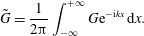 $$\begin{eqnarray}\tilde{G}=\frac{1}{2\unicode[STIX]{x03C0}}\int _{-\infty }^{+\infty }G\text{e}^{-\text{i}kx}\,\text{d}x.\end{eqnarray}$$
We may replace
 $\unicode[STIX]{x1D714}$
in (2.1) with
 $\unicode[STIX]{x1D6FE}=\unicode[STIX]{x1D714}-\text{i}\unicode[STIX]{x1D716}$
, where
 $\unicode[STIX]{x1D716}\rightarrow 0^{+}$
(Lighthill Reference Lighthill1978). For a non-zero
 $\unicode[STIX]{x1D716}$
,
 $G\rightarrow 0$
when
 $|x|\rightarrow \infty$
, and the radiation condition in (2.7) will be satisfied when
 $\unicode[STIX]{x1D716}$
is taken to be zero. Applying (3.2) to (3.1), we obtain
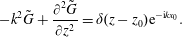 $$\begin{eqnarray}-k^{2}\tilde{G}+\frac{\unicode[STIX]{x2202}^{2}\tilde{G}}{\unicode[STIX]{x2202}z^{2}}=\unicode[STIX]{x1D6FF}(z-z_{0})\text{e}^{-\text{i}kx_{0}}.\end{eqnarray}$$
Here we introduce
 $$\begin{eqnarray}z_{{>}}=\max (z,z_{0})\quad \text{and}\quad z_{{<}}=\min (z,z_{0}).\end{eqnarray}$$
Then the solution for (3.3) with the boundary condition in (2.6) can be written in the following form
 $$\begin{eqnarray}\tilde{G}=\frac{\text{e}^{-\text{i}kx_{0}}}{k}[\unicode[STIX]{x1D6FC}k\cosh (kz_{{>}})+\unicode[STIX]{x1D6FD}\sinh (kz_{{>}})]Z(z_{{<}}),\end{eqnarray}$$
where
 $\unicode[STIX]{x1D6FC}$
and
 $\unicode[STIX]{x1D6FD}$
are two unknown constants to be solved,
 $$\begin{eqnarray}Z(z)=\cosh [k(z+H)].\end{eqnarray}$$
Integrating (3.3) with respect to
 $z$
from
 $z_{0}^{-}$
to
 $z_{0}^{+}$
, we have
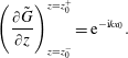 $$\begin{eqnarray}\left(\frac{\unicode[STIX]{x2202}\tilde{G}}{\unicode[STIX]{x2202}z}\right)_{z=z_{0}^{-}}^{z=z_{0}^{+}}=\text{e}^{-\text{i}kx_{0}}.\end{eqnarray}$$
Substituting (3.5) into (3.7), we obtain
 $$\begin{eqnarray}-\unicode[STIX]{x1D6FC}k\sinh (kH)+\unicode[STIX]{x1D6FD}\cosh (kH)=1.\end{eqnarray}$$
Fourier transform can also be applied to the boundary condition on the ice sheet in (2.3). We have
 $$\begin{eqnarray}\tilde{U} +(\unicode[STIX]{x1D70C}g-m\unicode[STIX]{x1D6FE}^{2})\frac{\unicode[STIX]{x2202}\tilde{G}}{\unicode[STIX]{x2202}z}-\unicode[STIX]{x1D70C}\unicode[STIX]{x1D6FE}^{2}\tilde{G}=0,\end{eqnarray}$$
where
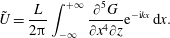 $$\begin{eqnarray}\tilde{U} =\frac{L}{2\unicode[STIX]{x03C0}}\int _{-\infty }^{+\infty }\frac{\unicode[STIX]{x2202}^{5}G}{\unicode[STIX]{x2202}x^{4}\unicode[STIX]{x2202}z}\text{e}^{-\text{i}kx}\,\text{d}x.\end{eqnarray}$$
Through integrating by parts and using the condition of
 $G\rightarrow 0$
at
 $|x|\rightarrow \infty$
when
 $\unicode[STIX]{x1D716}$
is non-zero, (3.10) can be given as
 $$\begin{eqnarray}\tilde{U} =\frac{L}{2\unicode[STIX]{x03C0}}\left[\left(\frac{\unicode[STIX]{x2202}^{4}G}{\unicode[STIX]{x2202}x^{3}\unicode[STIX]{x2202}z}+\text{i}k\frac{\unicode[STIX]{x2202}^{3}G}{\unicode[STIX]{x2202}x^{2}\unicode[STIX]{x2202}z}-k^{2}\frac{\unicode[STIX]{x2202}^{2}G}{\unicode[STIX]{x2202}x\unicode[STIX]{x2202}z}-\text{i}k^{3}\frac{\unicode[STIX]{x2202}G}{\unicode[STIX]{x2202}z}\right)\text{e}^{-\text{i}kx}\right]_{x=0^{+}}^{x=0^{-}}+Lk^{4}\frac{\unicode[STIX]{x2202}\tilde{G}}{\unicode[STIX]{x2202}z}.\end{eqnarray}$$
At the ice crack, we have condition (2.4). It is expected that the displacements and the slopes on both sides of the crack are discontinuous. Thus we may write
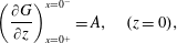 $$\begin{eqnarray}\displaystyle & \displaystyle \left(\frac{\unicode[STIX]{x2202}G}{\unicode[STIX]{x2202}z}\right)_{x=0^{+}}^{x=0^{-}}=A,\quad (z=0), & \displaystyle\end{eqnarray}$$
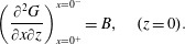 $$\begin{eqnarray}\displaystyle & \displaystyle \left(\frac{\unicode[STIX]{x2202}^{2}G}{\unicode[STIX]{x2202}x\unicode[STIX]{x2202}z}\right)_{x=0^{+}}^{x=0^{-}}=B,\quad (z=0). & \displaystyle\end{eqnarray}$$
Then (3.11) can be written as
 $$\begin{eqnarray}\tilde{U} =-\frac{L}{2\unicode[STIX]{x03C0}}(\text{i}k^{3}A+k^{2}B)+Lk^{4}\frac{\unicode[STIX]{x2202}\tilde{G}}{\unicode[STIX]{x2202}z}.\end{eqnarray}$$
It may be noticed that for crack conditions different from those in (3.12) and (3.13), a similar procedure may be followed, leading to a different form of (3.14). Substituting (3.5) together with (3.14) into (3.9) and invoking (3.8), we obtain
 $$\begin{eqnarray}\displaystyle & \displaystyle \unicode[STIX]{x1D6FC}=\frac{L}{2\unicode[STIX]{x03C0}}\frac{\text{i}k^{3}A+k^{2}B}{K(\unicode[STIX]{x1D6FE},k)Z(z_{0})}\text{e}^{\text{i}kx_{0}}-\frac{Lk^{4}+\unicode[STIX]{x1D70C}g-m\unicode[STIX]{x1D6FE}^{2}}{K(\unicode[STIX]{x1D6FE},k)Z(0)}, & \displaystyle\end{eqnarray}$$
 $$\begin{eqnarray}\displaystyle & \displaystyle \unicode[STIX]{x1D6FD}=\frac{L}{2\unicode[STIX]{x03C0}}\frac{(\text{i}k^{3}A+k^{2}B)Z^{\prime }(0)}{K(\unicode[STIX]{x1D6FE},k)Z(z_{0})Z(0)}\text{e}^{\text{i}kx_{0}}-\frac{\unicode[STIX]{x1D70C}\unicode[STIX]{x1D6FE}^{2}}{K(\unicode[STIX]{x1D6FE},k)Z(0)}, & \displaystyle\end{eqnarray}$$
where the prime denotes partial derivative with respect to
 $z$
. Substituting (3.15) and (3.16) into (3.5), we have
 $$\begin{eqnarray}\displaystyle \tilde{G} & = & \displaystyle -\frac{\text{e}^{-\text{i}kx_{0}}}{k}\frac{(Lk^{4}+\unicode[STIX]{x1D70C}g-m\unicode[STIX]{x1D6FE}^{2})k\cosh (kz_{{>}})+\unicode[STIX]{x1D70C}\unicode[STIX]{x1D6FE}^{2}\sinh (kz_{{>}})}{K(\unicode[STIX]{x1D6FE},k)Z(0)}Z(z_{{<}})\nonumber\\ \displaystyle & & \displaystyle +\,\frac{L}{2\unicode[STIX]{x03C0}}\frac{(\text{i}k^{3}A+k^{2}B)[\cosh (kz_{{>}})+\tanh (kH)\sinh (kz_{{>}})]}{K(\unicode[STIX]{x1D6FE},k)Z(z_{0})}Z(z_{{<}}).\end{eqnarray}$$
Using
 $$\begin{eqnarray}\displaystyle & \displaystyle \ln \left(\frac{r_{1}}{H}\right)=\int _{0}^{+\infty }\frac{\text{e}^{-kH}-\text{e}^{-k(z_{{>}}-z_{{<}})}\cos [k(x-x_{0})]}{k}\,\text{d}k, & \displaystyle\end{eqnarray}$$
 $$\begin{eqnarray}\displaystyle & \displaystyle \ln \left(\frac{r_{2}}{H}\right)=\int _{0}^{+\infty }\frac{\text{e}^{-kH}-\text{e}^{-k(z_{{>}}+z_{{<}}+2H)}\cos [k(x-x_{0})]}{k}\,\text{d}k, & \displaystyle\end{eqnarray}$$
where
 $r_{1}$
is the distance between
 $p$
and
 $q$
, and
 $r_{2}$
is the distance between
 $p$
and the mirror image of
 $q$
about the flat seabed
 $z=-H$
, and then performing the inverse Fourier transform of
 $\tilde{G}$
, the solution due to a single source can be written as
 $$\begin{eqnarray}G=G_{ice}(x,z;x_{0},z_{0})+A\times \frac{\unicode[STIX]{x2202}G_{1}(x,z)}{\unicode[STIX]{x2202}x}+B\times G_{1}(x,z),\end{eqnarray}$$
where
 $$\begin{eqnarray}G_{ice}=\ln \left(\frac{r_{1}}{H}\right)+\ln \left(\frac{r_{2}}{H}\right)-2\int _{0}^{+\infty }\frac{\text{e}^{-kH}}{k}\{P(k)Z(z)Z(z_{0})\cos [k(x-x_{0})]+1\}\,\text{d}k,\end{eqnarray}$$
with
 $$\begin{eqnarray}P(k)=\frac{(Lk^{4}+\unicode[STIX]{x1D70C}g-m\unicode[STIX]{x1D6FE}^{2})k+\unicode[STIX]{x1D70C}\unicode[STIX]{x1D6FE}^{2}}{K(\unicode[STIX]{x1D6FE},k)Z(0)},\end{eqnarray}$$
and
 $$\begin{eqnarray}G_{1}=\frac{L}{\unicode[STIX]{x03C0}}\int _{0}^{+\infty }\frac{Z(z)}{K(\unicode[STIX]{x1D6FE},k)Z(0)}k^{2}\cos (kx)\,\text{d}k.\end{eqnarray}$$
We may notice that
 $G_{ice}$
is in fact the Green function without the crack (Evans & Porter Reference Evans and Porter2003). We may also notice that
 $G_{1}$
satisfies (2.3) and
 $$\begin{eqnarray}G_{1}(x,z)=\frac{L}{2\unicode[STIX]{x03C0}\unicode[STIX]{x1D70C}\unicode[STIX]{x1D6FE}^{2}}\left(\frac{\unicode[STIX]{x2202}^{3}G_{ice}(x_{0},z_{0};x,z)}{\unicode[STIX]{x2202}z_{0}\unicode[STIX]{x2202}x_{0}^{2}}\right)_{x_{0}=0,z_{0}=0}.\end{eqnarray}$$
For the current problem with a crack, there are still two unknown coefficients,
 $A$
and
 $B$
in (3.20), which can be determined by the condition in (2.4). The zero bending moment and shear force conditions respectively give
 $$\begin{eqnarray}\displaystyle & \displaystyle \lim _{x,z\rightarrow 0}G_{zxx}=\frac{2\unicode[STIX]{x03C0}\unicode[STIX]{x1D70C}\unicode[STIX]{x1D6FE}^{2}}{L}G_{1}(x_{0},z_{0})+A\lim _{x,z\rightarrow 0}\frac{\unicode[STIX]{x2202}^{4}G_{1}(x,z)}{\unicode[STIX]{x2202}z\unicode[STIX]{x2202}x^{3}}+B\lim _{x,z\rightarrow 0}\frac{\unicode[STIX]{x2202}^{3}G_{1}(x,z)}{\unicode[STIX]{x2202}z\unicode[STIX]{x2202}x^{2}}=0,\qquad & \displaystyle\end{eqnarray}$$
 $$\begin{eqnarray}\displaystyle & \displaystyle \lim _{x,z\rightarrow 0}G_{zxxx}=-\frac{2\unicode[STIX]{x03C0}\unicode[STIX]{x1D70C}\unicode[STIX]{x1D6FE}^{2}}{L}\frac{\unicode[STIX]{x2202}G_{1}(x_{0},z_{0})}{\unicode[STIX]{x2202}x_{0}}+A\lim _{x,z\rightarrow 0}\frac{\unicode[STIX]{x2202}^{5}G_{1}(x,z)}{\unicode[STIX]{x2202}z\unicode[STIX]{x2202}x^{4}}+B\lim _{x,z\rightarrow 0}\frac{\unicode[STIX]{x2202}^{4}G_{1}(x,z)}{\unicode[STIX]{x2202}z\unicode[STIX]{x2202}x^{3}}=0,\qquad & \displaystyle\end{eqnarray}$$
where (3.24) has been used. We then notice that when
 $x=r\sin \unicode[STIX]{x1D6E9}$
and
 $z=-r\cos \unicode[STIX]{x1D6E9}$
we have at
 $z<0$
 $$\begin{eqnarray}\frac{\text{e}^{\text{i}(m+1)\unicode[STIX]{x1D6E9}}}{r^{m+1}}=\frac{1}{m!}\int _{0}^{+\infty }\text{e}^{kz}k^{m}\text{e}^{\text{i}kx}\,\text{d}k.\end{eqnarray}$$
This means that when
 $\unicode[STIX]{x1D6E9}\rightarrow \unicode[STIX]{x03C0}/2$
, or
 $z\rightarrow 0$
, we have
 $$\begin{eqnarray}\lim _{z\rightarrow 0}\int _{0}^{+\infty }\text{e}^{kz}k^{m}\cos (kx)\,\text{d}k=0\quad \text{for an even }m,\end{eqnarray}$$
and
 $$\begin{eqnarray}\lim _{z\rightarrow 0}\int _{0}^{+\infty }\text{e}^{kz}k^{m}\sin (kx)\,\text{d}k=0\quad \text{for an odd }m.\end{eqnarray}$$
Equations (3.28) and (3.29) further provide
 $$\begin{eqnarray}\lim _{z\rightarrow 0}\int _{0}^{+\infty }\frac{Z^{\prime }(z)}{Z^{\prime }(0)}k^{m}\cos (kx)\,\text{d}k=0\quad \text{for an even }m,\end{eqnarray}$$
and
 $$\begin{eqnarray}\lim _{z\rightarrow 0}\int _{0}^{+\infty }\frac{Z^{\prime }(z)}{Z^{\prime }(0)}k^{m}\sin (kx)\,\text{d}k=0\quad \text{for an odd }m.\end{eqnarray}$$
Using these two equations, we have
 $$\begin{eqnarray}\displaystyle & \displaystyle \lim _{z\rightarrow 0}\frac{\unicode[STIX]{x2202}^{3}G_{1}(x,z)}{\unicode[STIX]{x2202}z\unicode[STIX]{x2202}x^{2}}=-\frac{1}{\unicode[STIX]{x03C0}}\int _{0}^{+\infty }\frac{\unicode[STIX]{x1D70C}\unicode[STIX]{x1D6FE}^{2}-(\unicode[STIX]{x1D70C}g-m\unicode[STIX]{x1D6FE}^{2})k\tanh (kH)}{K(\unicode[STIX]{x1D6FE},k)}\cos (kx)\,\text{d}k, & \displaystyle\end{eqnarray}$$
 $$\begin{eqnarray}\displaystyle & \displaystyle \lim _{z\rightarrow 0}\frac{\unicode[STIX]{x2202}^{4}G_{1}(x,z)}{\unicode[STIX]{x2202}z\unicode[STIX]{x2202}x^{3}}=\frac{1}{\unicode[STIX]{x03C0}}\int _{0}^{+\infty }\frac{\unicode[STIX]{x1D70C}\unicode[STIX]{x1D6FE}^{2}-(\unicode[STIX]{x1D70C}g-m\unicode[STIX]{x1D6FE}^{2})k\tanh (kH)}{K(\unicode[STIX]{x1D6FE},k)}k\sin (kx)\,\text{d}k, & \displaystyle\end{eqnarray}$$
 $$\begin{eqnarray}\displaystyle & \displaystyle \lim _{z\rightarrow 0}\frac{\unicode[STIX]{x2202}^{5}G_{1}(x,z)}{\unicode[STIX]{x2202}z\unicode[STIX]{x2202}x^{4}}=\frac{1}{\unicode[STIX]{x03C0}}\int _{0}^{+\infty }\frac{\unicode[STIX]{x1D70C}\unicode[STIX]{x1D6FE}^{2}-(\unicode[STIX]{x1D70C}g-m\unicode[STIX]{x1D6FE}^{2})k\tanh (kH)}{K(\unicode[STIX]{x1D6FE},k)}k^{2}\cos (kx)\,\text{d}k. & \displaystyle\end{eqnarray}$$
Through these results, (3.26) and (3.25) then respectively give
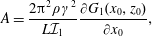 $$\begin{eqnarray}A=\frac{2\unicode[STIX]{x03C0}^{2}\unicode[STIX]{x1D70C}\unicode[STIX]{x1D6FE}^{2}}{L{\mathcal{I}}_{1}}\frac{\unicode[STIX]{x2202}G_{1}(x_{0},z_{0})}{\unicode[STIX]{x2202}x_{0}},\end{eqnarray}$$
and
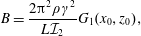 $$\begin{eqnarray}B=\frac{2\unicode[STIX]{x03C0}^{2}\unicode[STIX]{x1D70C}\unicode[STIX]{x1D6FE}^{2}}{L{\mathcal{I}}_{2}}G_{1}(x_{0},z_{0}),\end{eqnarray}$$
where
 $$\begin{eqnarray}\displaystyle & \displaystyle {\mathcal{I}}_{1}=\unicode[STIX]{x03C0}\lim _{x,z\rightarrow 0}\frac{\unicode[STIX]{x2202}^{5}G_{1}(x,z)}{\unicode[STIX]{x2202}z\unicode[STIX]{x2202}x^{4}}=\int _{0}^{+\infty }\frac{\unicode[STIX]{x1D70C}\unicode[STIX]{x1D6FE}^{2}-(\unicode[STIX]{x1D70C}g-m\unicode[STIX]{x1D6FE}^{2})k\tanh (kH)}{K(\unicode[STIX]{x1D6FE},k)}k^{2}\,\text{d}k, & \displaystyle\end{eqnarray}$$
 $$\begin{eqnarray}\displaystyle & \displaystyle {\mathcal{I}}_{2}=-\unicode[STIX]{x03C0}\lim _{x,z\rightarrow 0}\frac{\unicode[STIX]{x2202}^{3}G_{1}(x,z)}{\unicode[STIX]{x2202}z\unicode[STIX]{x2202}x^{2}}=\int _{0}^{+\infty }\frac{\unicode[STIX]{x1D70C}\unicode[STIX]{x1D6FE}^{2}-(\unicode[STIX]{x1D70C}g-m\unicode[STIX]{x1D6FE}^{2})k\tanh (kH)}{K(\unicode[STIX]{x1D6FE},k)}\,\text{d}k. & \displaystyle\end{eqnarray}$$
 $$\begin{eqnarray}G=G_{ice}(x,z;x_{0},z_{0})+\frac{2\unicode[STIX]{x03C0}^{2}\unicode[STIX]{x1D70C}\unicode[STIX]{x1D6FE}^{2}}{L}\left[\frac{1}{{\mathcal{I}}_{1}}\frac{\unicode[STIX]{x2202}G_{1}(x,z)}{\unicode[STIX]{x2202}x}\frac{\unicode[STIX]{x2202}G_{1}(x_{0},z_{0})}{\unicode[STIX]{x2202}x_{0}}+\frac{G_{1}(x,z)G_{1}(x_{0},z_{0})}{{\mathcal{I}}_{2}}\right].\end{eqnarray}$$
The replacement of
 $\unicode[STIX]{x1D714}$
with
 $\unicode[STIX]{x1D6FE}=\unicode[STIX]{x1D714}-\text{i}\unicode[STIX]{x1D716}$
in (2.8) during the derivation moves the pole
 $k=\unicode[STIX]{x1D706}$
off the real axis of
 $k$
. Letting
 $\unicode[STIX]{x1D716}\rightarrow 0^{+}$
, the Taylor expansion of the dispersion equation
 $K(\unicode[STIX]{x1D6FE},k)$
with respect to
 $\unicode[STIX]{x1D716}$
provides the root at
 $$\begin{eqnarray}k=\unicode[STIX]{x1D706}-\text{i}\unicode[STIX]{x1D716}^{\prime },\end{eqnarray}$$
where
 $$\begin{eqnarray}\unicode[STIX]{x1D716}^{\prime }=\frac{\unicode[STIX]{x1D716}}{\unicode[STIX]{x1D714}}\frac{L\unicode[STIX]{x1D706}^{4}+\unicode[STIX]{x1D70C}g}{L\unicode[STIX]{x1D706}^{4}+\unicode[STIX]{x1D70C}g-m\unicode[STIX]{x1D714}^{2}}\left/\left[\frac{1}{2\unicode[STIX]{x1D706}}+\frac{H}{\sinh (2\unicode[STIX]{x1D706}H)}+\frac{2L\unicode[STIX]{x1D706}^{3}}{L\unicode[STIX]{x1D706}^{4}+\unicode[STIX]{x1D70C}g-m\unicode[STIX]{x1D714}^{2}}\right]\right..\end{eqnarray}$$
Thus when
 $\unicode[STIX]{x1D716}\rightarrow 0^{+}$
, the pole will approach the real axis of
 $k$
from below. Therefore, the integration route
 ${\mathcal{D}}$
in (3.38) from
 $0$
to
 $+\infty$
should pass over the pole at
 $k=\unicode[STIX]{x1D706}$
, which is consistent with the radiation condition, i.e. the wave will propagate away from the source into infinity. With such a definition of
 ${\mathcal{D}}$
,
 $\unicode[STIX]{x1D6FE}$
in (3.38) can be replaced by
 $\unicode[STIX]{x1D714}$
. We may notice that (3.38) is a summation of the Green function
 $G_{ice}$
for the ice sheet without the crack and two additional terms equivalent to the loads applied at the crack to ensure that the shear force and bending moment there are zero. We may also notice that the integrand of
 $G$
in (3.38) has only a simple pole at
 $k=\unicode[STIX]{x1D706}$
where
 $K(\unicode[STIX]{x1D714},k)=0$
. The integration may be calculated by using the Gauss–Legendre principal value integration procedure (Noble Reference Noble2000). This may also be done by following the numerical procedure in Wu & Eatock Taylor (Reference Wu and Eatock Taylor1987), which effectively removes the singularity.
3.2 Multipole expansion
Potentials due to multipoles or singularities of higher order may be found by differentiating (3.38) with respect to the position of the source point. In such a way, none of the boundary conditions will be affected and will be still satisfied. As shown in figure 1, we have
 $x-x_{0}=r\sin \unicode[STIX]{x1D703}$
and
 $z-z_{0}=r\cos \unicode[STIX]{x1D703}$
. Similar to Wu (Reference Wu1998), we may apply the operator
 $$\begin{eqnarray}(D_{\pm })^{n}=-\frac{1}{2^{n-1}(n-1)!}\left(\frac{\unicode[STIX]{x2202}}{\unicode[STIX]{x2202}z_{0}}\pm \text{i}\frac{\unicode[STIX]{x2202}}{\unicode[STIX]{x2202}x_{0}}\right)^{n}\end{eqnarray}$$
to (3.38). Using the result
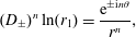 $$\begin{eqnarray}(D_{\pm })^{n}\ln (r_{1})=\frac{\text{e}^{\pm \text{i}n\unicode[STIX]{x1D703}}}{r^{n}},\end{eqnarray}$$
and noticing
 $(D_{+})\exp (\pm kz_{0}\pm \text{i}kx_{0})=0$
and
 $(D_{-})\exp (\pm kz_{0}\mp \text{i}kx_{0})=0$
, we have
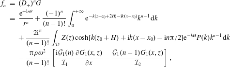 $$\begin{eqnarray}\displaystyle f_{n} & = & \displaystyle (D_{+})^{n}G\nonumber\\ \displaystyle & = & \displaystyle \frac{\text{e}^{+\text{i}n\unicode[STIX]{x1D703}}}{r^{n}}+\frac{(-1)^{n}}{(n-1)!}\int _{0}^{+\infty }\text{e}^{-k(z+z_{0}+2H)-\text{i}k(x-x_{0})}k^{n-1}\,\text{d}k\nonumber\\ \displaystyle & & \displaystyle +\,\frac{2\text{i}^{n}}{(n-1)!}\int _{{\mathcal{D}}}Z(z)\cosh [k(z_{0}+H)+\text{i}k(x-x_{0})-\text{i}n\unicode[STIX]{x03C0}/2]\text{e}^{-kH}P(k)k^{n-1}\,\text{d}k\nonumber\\ \displaystyle & & \displaystyle -\,\frac{\unicode[STIX]{x03C0}\unicode[STIX]{x1D70C}\unicode[STIX]{x1D714}^{2}}{(n-1)!}\left[\frac{\text{i}{\mathcal{G}}_{1}(n)}{{\mathcal{I}}_{1}}\frac{\unicode[STIX]{x2202}G_{1}(x,z)}{\unicode[STIX]{x2202}x}-\frac{{\mathcal{G}}_{1}(n-1)G_{1}(x,z)}{{\mathcal{I}}_{2}}\right],\end{eqnarray}$$
and
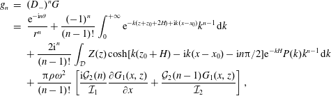 $$\begin{eqnarray}\displaystyle g_{n} & = & \displaystyle (D_{-})^{n}G\nonumber\\ \displaystyle & = & \displaystyle \frac{\text{e}^{-\text{i}n\unicode[STIX]{x1D703}}}{r^{n}}+\frac{(-1)^{n}}{(n-1)!}\int _{0}^{+\infty }\text{e}^{-k(z+z_{0}+2H)+\text{i}k(x-x_{0})}k^{n-1}\,\text{d}k\nonumber\\ \displaystyle & & \displaystyle +\,\frac{2\text{i}^{n}}{(n-1)!}\int _{{\mathcal{D}}}Z(z)\cosh [k(z_{0}+H)-\text{i}k(x-x_{0})-\text{i}n\unicode[STIX]{x03C0}/2]\text{e}^{-kH}P(k)k^{n-1}\,\text{d}k\nonumber\\ \displaystyle & & \displaystyle +\,\frac{\unicode[STIX]{x03C0}\unicode[STIX]{x1D70C}\unicode[STIX]{x1D714}^{2}}{(n-1)!}\left[\frac{\text{i}{\mathcal{G}}_{2}(n)}{{\mathcal{I}}_{1}}\frac{\unicode[STIX]{x2202}G_{1}(x,z)}{\unicode[STIX]{x2202}x}+\frac{{\mathcal{G}}_{2}(n-1)G_{1}(x,z)}{{\mathcal{I}}_{2}}\right],\end{eqnarray}$$
where
 $$\begin{eqnarray}\displaystyle & \displaystyle {\mathcal{G}}_{1}(n)=\int _{{\mathcal{D}}}\frac{(-1)^{n}\text{e}^{-k(z_{0}+H)+\text{i}kx_{0}}-\text{e}^{k(z_{0}+H)-\text{i}kx_{0}}}{K(\unicode[STIX]{x1D714},k)Z(0)}k^{n+3}\,\text{d}k, & \displaystyle\end{eqnarray}$$
 $$\begin{eqnarray}\displaystyle & \displaystyle {\mathcal{G}}_{2}(n)=\int _{{\mathcal{D}}}\frac{(-1)^{n}\text{e}^{-k(z_{0}+H)-\text{i}kx_{0}}-\text{e}^{k(z_{0}+H)+\text{i}kx_{0}}}{K(\unicode[STIX]{x1D714},k)Z(0)}k^{n+3}\,\text{d}k. & \displaystyle\end{eqnarray}$$
 $\text{i}$
in (3.43) is replaced by
 $-\text{i}$
,
 $f_{n}$
becomes
 $g_{n}$
.
3.3 Solution for the radiation problem
Here we consider the wave radiation due to the body undergoing sinusoidal oscillation with frequency
 $\unicode[STIX]{x1D714}$
. By using (3.43) and (3.44), we can write the potentials
 $\unicode[STIX]{x1D719}_{j}$
in terms of multipole expansions in the polar coordinate system as
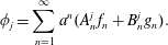 $$\begin{eqnarray}\unicode[STIX]{x1D719}_{j}=\mathop{\sum }_{n=1}^{\infty }a^{n}(A_{n}^{j}\,f_{n}+B_{n}^{j}g_{n}).\end{eqnarray}$$
 $\unicode[STIX]{x1D719}_{j}$
now satisfies the governing equation and all the boundary conditions apart from that on the body surface, which is to be used to obtain the coefficients
 $A_{n}^{j}$
and
 $B_{n}^{j}$
. When
 $j=1,2$
, we respectively have
 $$\begin{eqnarray}\frac{\unicode[STIX]{x2202}\unicode[STIX]{x1D719}_{1}}{\unicode[STIX]{x2202}r}=-\frac{\unicode[STIX]{x2202}\unicode[STIX]{x1D719}_{1}}{\unicode[STIX]{x2202}n}=\sin \unicode[STIX]{x1D703}\quad \text{and}\quad \frac{\unicode[STIX]{x2202}\unicode[STIX]{x1D719}_{2}}{\unicode[STIX]{x2202}r}=-\frac{\unicode[STIX]{x2202}\unicode[STIX]{x1D719}_{2}}{\unicode[STIX]{x2202}n}=\cos \unicode[STIX]{x1D703},\quad (r=a),\end{eqnarray}$$
where the minus sign is due to the fact that
 $\boldsymbol{n}$
points into the body. Since
 $$\begin{eqnarray}\text{e}^{kz\pm \text{i}kx}=\exp (kz_{0}\pm \text{i}kx_{0}+kr\text{e}^{\pm \text{i}\unicode[STIX]{x1D703}})=\text{e}^{kz_{0}\pm \text{i}kx_{0}}\mathop{\sum }_{l=0}^{\infty }\frac{k^{l}r^{l}\text{e}^{\pm \text{i}l\unicode[STIX]{x1D703}}}{l!},\end{eqnarray}$$
 $\unicode[STIX]{x1D719}_{j}$
can be expressed in the polar coordinate system as
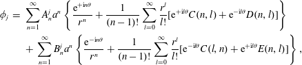 $$\begin{eqnarray}\displaystyle \unicode[STIX]{x1D719}_{j} & = & \displaystyle \mathop{\sum }_{n=1}^{\infty }A_{n}^{j}a^{n}\left\{\frac{\text{e}^{+\text{i}n\unicode[STIX]{x1D703}}}{r^{n}}+\frac{1}{(n-1)!}\mathop{\sum }_{l=0}^{\infty }\frac{r^{l}}{l!}[\text{e}^{+\text{i}l\unicode[STIX]{x1D703}}C(n,l)+\text{e}^{-\text{i}l\unicode[STIX]{x1D703}}D(n,l)]\right\}\nonumber\\ \displaystyle & & \displaystyle +\,\mathop{\sum }_{n=1}^{\infty }B_{n}^{j}a^{n}\left\{\frac{\text{e}^{-\text{i}n\unicode[STIX]{x1D703}}}{r^{n}}+\frac{1}{(n-1)!}\mathop{\sum }_{l=0}^{\infty }\frac{r^{l}}{l!}[\text{e}^{-\text{i}l\unicode[STIX]{x1D703}}C(l,n)+\text{e}^{+\text{i}l\unicode[STIX]{x1D703}}E(n,l)]\right\},\end{eqnarray}$$
where
 $$\begin{eqnarray}\displaystyle & \displaystyle C(n,l)=(-1)^{n+l}{\mathcal{J}}_{1}(n+l)+\frac{{\mathcal{J}}_{3}(n+l)}{2}-\frac{L\unicode[STIX]{x1D70C}\unicode[STIX]{x1D714}^{2}}{4}\left[\frac{{\mathcal{G}}_{1}(n){\mathcal{G}}_{2}(l)}{{\mathcal{I}}_{1}}+\frac{{\mathcal{G}}_{1}(n-1){\mathcal{G}}_{2}(l-1)}{{\mathcal{I}}_{2}}\right], & \displaystyle \nonumber\\ \displaystyle & & \displaystyle\end{eqnarray}$$
 $$\begin{eqnarray}\displaystyle & \displaystyle D(n,l)=[(-1)^{l}+(-1)^{n}]\frac{{\mathcal{J}}_{2}(n+l)}{2}+\frac{L\unicode[STIX]{x1D70C}\unicode[STIX]{x1D714}^{2}}{4}\left[\frac{{\mathcal{G}}_{1}(n){\mathcal{G}}_{1}(l)}{{\mathcal{I}}_{1}}-\frac{{\mathcal{G}}_{1}(n-1){\mathcal{G}}_{1}(l-1)}{{\mathcal{I}}_{2}}\right], & \displaystyle \nonumber\\ \displaystyle & & \displaystyle\end{eqnarray}$$
 $$\begin{eqnarray}\displaystyle & \displaystyle E(n,l)=[(-1)^{l}+(-1)^{n}]\frac{{\mathcal{J}}_{2}(n+l)}{2}+\frac{L\unicode[STIX]{x1D70C}\unicode[STIX]{x1D714}^{2}}{4}\left[\frac{{\mathcal{G}}_{2}(n){\mathcal{G}}_{2}(l)}{{\mathcal{I}}_{1}}-\frac{{\mathcal{G}}_{2}(n-1){\mathcal{G}}_{2}(l-1)}{{\mathcal{I}}_{2}}\right], & \displaystyle \nonumber\\ \displaystyle & & \displaystyle\end{eqnarray}$$
 $$\begin{eqnarray}\displaystyle & \displaystyle {\mathcal{J}}_{1}(n)=\unicode[STIX]{x1D6E4}(n)/[2(z_{0}+H)]^{n}, & \displaystyle\end{eqnarray}$$
 $$\begin{eqnarray}\displaystyle & \displaystyle {\mathcal{J}}_{2}(n)=\int _{{\mathcal{D}}}\text{e}^{-kH}P(k)k^{n-1}\,\text{d}k, & \displaystyle\end{eqnarray}$$
 $$\begin{eqnarray}\displaystyle & \displaystyle {\mathcal{J}}_{3}(n)=\int _{{\mathcal{D}}}[(-1)^{n}\text{e}^{-2k(z_{0}+H)}+\text{e}^{2k(z_{0}+H)}]\text{e}^{-kH}P(k)k^{n-1}\,\text{d}k. & \displaystyle\end{eqnarray}$$
 $\unicode[STIX]{x1D6E4}(n)$
is the gamma function (Abramowitz & Stegun Reference Abramowitz and Stegun1965). Invoking (3.47), then using the orthogonality of trigonometric function, we have
 $$\begin{eqnarray}-l\frac{A_{l}^{j}}{a}+\mathop{\sum }_{n=1}^{\infty }\frac{A_{n}^{j}a^{n+l-1}C(n,l)}{(n-1)!(l-1)!}+\mathop{\sum }_{n=1}^{\infty }\frac{B_{n}^{j}a^{n+l-1}E(n,l)}{(n-1)!(l-1)!}=u_{l}(j),\end{eqnarray}$$
and
 $$\begin{eqnarray}-l\frac{B_{l}^{j}}{a}+\mathop{\sum }_{n=1}^{\infty }\frac{B_{n}^{j}a^{n+l-1}C(l,n)}{(n-1)!(l-1)!}+\mathop{\sum }_{n=1}^{\infty }\frac{A_{n}^{j}a^{n+l-1}D(n,l)}{(n-1)!(l-1)!}=v_{l}(j),\end{eqnarray}$$
for
 $l=1,2,\ldots \,$
, where
 $$\begin{eqnarray}u_{l}(1)={\textstyle \frac{1}{2\text{i}}}\unicode[STIX]{x1D6FF}_{l1},\quad v_{l}(1)=-u_{l}(1),\end{eqnarray}$$
and
 $$\begin{eqnarray}u_{l}(2)={\textstyle \frac{1}{2}}\unicode[STIX]{x1D6FF}_{l1},\quad v_{l}(2)=u_{l}(2).\end{eqnarray}$$
Here
 $\unicode[STIX]{x1D6FF}_{l1}$
is the Kronecker delta function, and
 $j=1,2$
in (3.52) and (3.53) correspond to
 $\unicode[STIX]{x1D719}_{1}$
and
 $\unicode[STIX]{x1D719}_{2}$
respectively. For each
 $l$
, (3.52) and (3.53) provide two linear equations for
 $A_{n}^{j}$
and
 $B_{n}^{j}$
. Thus when the infinite summation is truncated at a finite number, we can obtain a matrix equation, from which
 $A_{n}^{j}$
and
 $B_{n}^{j}$
can be solved. When the solutions for
 $\unicode[STIX]{x1D719}_{1}$
and
 $\unicode[STIX]{x1D719}_{2}$
have been obtained, the added mass
 $\unicode[STIX]{x1D707}_{js}$
and damping coefficients
 $\unicode[STIX]{x1D706}_{js}$
can be computed through (Newman Reference Newman1977)
 $$\begin{eqnarray}\unicode[STIX]{x1D70F}_{js}=\unicode[STIX]{x1D707}_{js}-\text{i}\frac{\unicode[STIX]{x1D706}_{js}}{\unicode[STIX]{x1D714}}=\unicode[STIX]{x1D70C}\int _{S_{0}}\unicode[STIX]{x1D719}_{s}n_{j}\,\text{d}S,\end{eqnarray}$$
for
 $j,s=1,2$
, where
 $S_{0}$
represents the body surface. Multiplying both sides of (3.52) and (3.53) respectively by
 $\text{e}^{+\text{i}l\unicode[STIX]{x1D703}}$
and
 $\text{e}^{-\text{i}l\unicode[STIX]{x1D703}}$
, then taking summation with respect to
 $l$
from
 $1$
to
 $+\infty$
, substituting the obtained results into (3.49), and letting
 $r=a$
, we have (Wu Reference Wu1993)
 $$\begin{eqnarray}\unicode[STIX]{x1D719}_{s}=2\mathop{\sum }_{n=1}^{\infty }[A_{n}^{s}\text{e}^{+\text{i}n\unicode[STIX]{x1D703}}+B_{n}^{s}\text{e}^{-\text{i}n\unicode[STIX]{x1D703}}]+a\mathop{\sum }_{n=1}^{\infty }\frac{1}{n}[\text{e}^{+\text{i}n\unicode[STIX]{x1D703}}u_{n}(s)+\text{e}^{-\text{i}n\unicode[STIX]{x1D703}}v_{n}(s)]+\unicode[STIX]{x1D719}_{c}^{s},\end{eqnarray}$$
where
 $$\begin{eqnarray}\unicode[STIX]{x1D719}_{c}^{s}=\mathop{\sum }_{n=1}^{\infty }\frac{A_{n}^{s}a^{n}}{(n-1)!}[C(n,0)+D(n,0)]+\mathop{\sum }_{n=1}^{\infty }\frac{B_{n}^{s}a^{n}}{(n-1)!}[C(0,n)+E(n,0)].\end{eqnarray}$$
Substituting (3.57) into (3.56), we obtain
 $$\begin{eqnarray}\unicode[STIX]{x1D70F}_{1s}=-\text{i}2\unicode[STIX]{x03C0}\unicode[STIX]{x1D70C}a(A_{1}^{s}-B_{1}^{s})-\unicode[STIX]{x1D6FF}_{1s}\unicode[STIX]{x03C0}\unicode[STIX]{x1D70C}a^{2},\end{eqnarray}$$
and
 $$\begin{eqnarray}\unicode[STIX]{x1D70F}_{2s}=-2\unicode[STIX]{x03C0}\unicode[STIX]{x1D70C}a(A_{1}^{s}+B_{1}^{s})-\unicode[STIX]{x1D6FF}_{2s}\unicode[STIX]{x03C0}\unicode[STIX]{x1D70C}a^{2}.\end{eqnarray}$$
3.4 Solution for the diffraction problem
Wave diffraction potential consists of two parts and the total diffraction potential
 $\unicode[STIX]{x1D719}_{D}$
can be written as
 $$\begin{eqnarray}\unicode[STIX]{x1D719}_{D}=\unicode[STIX]{x1D719}_{D}^{1}+\unicode[STIX]{x1D719}_{D}^{2},\end{eqnarray}$$
where
 $\unicode[STIX]{x1D719}_{D}^{1}$
is the diffraction potential by the crack to
 $\unicode[STIX]{x1D719}_{I}$
, and
 $\unicode[STIX]{x1D719}_{D}^{2}$
is the diffraction potential by the cylinder to
 $\unicode[STIX]{x1D711}=\unicode[STIX]{x1D719}_{I}+\unicode[STIX]{x1D719}_{D}^{1}$
. For a periodic wave from
 $x=-\infty$
to
 $x=+\infty$
,
 $\unicode[STIX]{x1D719}_{I}$
can be given as
 $$\begin{eqnarray}\unicode[STIX]{x1D719}_{I}=I\text{e}^{-\text{i}\unicode[STIX]{x1D706}x}\unicode[STIX]{x1D713}(z),\end{eqnarray}$$
with
 $$\begin{eqnarray}\unicode[STIX]{x1D713}(z)=\cosh [\unicode[STIX]{x1D706}(H+z)]/\text{cosh}(\unicode[STIX]{x1D706}H),\end{eqnarray}$$
and
 $I=g/\text{i}\unicode[STIX]{x1D714}$
. Applying the Green’s second identity to
 $\unicode[STIX]{x1D719}_{D}^{1}$
and
 $G$
in (3.38) over the fluid boundary
 $S$
, we have
 $$\begin{eqnarray}2\unicode[STIX]{x03C0}\unicode[STIX]{x1D719}_{D}^{1}(x,z)=\int _{S}\left[\unicode[STIX]{x1D719}_{D}^{1}(\unicode[STIX]{x1D709},\unicode[STIX]{x1D701})\frac{\unicode[STIX]{x2202}G(x,z;\unicode[STIX]{x1D709},\unicode[STIX]{x1D701})}{\unicode[STIX]{x2202}n}-G(x,z;\unicode[STIX]{x1D709},\unicode[STIX]{x1D701})\frac{\unicode[STIX]{x2202}\unicode[STIX]{x1D719}_{D}^{1}(\unicode[STIX]{x1D709},\unicode[STIX]{x1D701})}{\unicode[STIX]{x2202}n}\right]\,\text{d}S,\end{eqnarray}$$
where the derivative and integration are with respect to
 $(\unicode[STIX]{x1D709},\unicode[STIX]{x1D701})$
. Invoking the boundary conditions for
 $\unicode[STIX]{x1D719}_{D}^{1}$
and
 $G$
, only the ice sheet will remain on the right-hand side of (3.64). Using condition (2.3) and through integrating by parts, this equation can be further written as
 $$\begin{eqnarray}2\unicode[STIX]{x03C0}\unicode[STIX]{x1D719}_{D}^{1}=\frac{L}{\unicode[STIX]{x1D70C}\unicode[STIX]{x1D714}^{2}}\left[\left(\frac{\unicode[STIX]{x2202}^{4}\unicode[STIX]{x1D719}_{D}^{1}}{\unicode[STIX]{x2202}\unicode[STIX]{x1D709}^{3}\unicode[STIX]{x2202}\unicode[STIX]{x1D701}}\frac{\unicode[STIX]{x2202}G}{\unicode[STIX]{x2202}\unicode[STIX]{x1D701}}-\frac{\unicode[STIX]{x2202}^{3}\unicode[STIX]{x1D719}_{D}^{1}}{\unicode[STIX]{x2202}\unicode[STIX]{x1D709}^{2}\unicode[STIX]{x2202}\unicode[STIX]{x1D701}}\frac{\unicode[STIX]{x2202}^{2}G}{\unicode[STIX]{x2202}\unicode[STIX]{x1D709}\unicode[STIX]{x2202}\unicode[STIX]{x1D701}}\right)_{\unicode[STIX]{x1D709}=0^{+}}^{\unicode[STIX]{x1D709}=0^{-}}\right]_{\unicode[STIX]{x1D701}=0}.\end{eqnarray}$$
Noticing that
 $\unicode[STIX]{x1D711}=\unicode[STIX]{x1D719}_{I}+\unicode[STIX]{x1D719}_{D}^{1}$
should satisfy the crack condition in (2.4), then
 $\unicode[STIX]{x1D719}_{D}^{1}(x,z)$
can be obtained directly through the Green function as
 $$\begin{eqnarray}\unicode[STIX]{x1D719}_{D}^{1}=-\unicode[STIX]{x03C0}I\unicode[STIX]{x1D706}^{3}\tanh (\unicode[STIX]{x1D706}H)\left[\frac{\text{i}\unicode[STIX]{x1D706}}{{\mathcal{I}}_{1}}\frac{\unicode[STIX]{x2202}G_{1}(x,z)}{\unicode[STIX]{x2202}x}+\frac{G_{1}(x,z)}{{\mathcal{I}}_{2}}\right].\end{eqnarray}$$
To obtain the solution for
 $\unicode[STIX]{x1D719}_{D}^{2}$
,
 $\unicode[STIX]{x1D711}=\unicode[STIX]{x1D719}_{I}+\unicode[STIX]{x1D719}_{D}^{1}$
can be expressed in the polar coordinate system through using (3.48)
 $$\begin{eqnarray}\unicode[STIX]{x1D711}=I\mathop{\sum }_{n=0}^{\infty }\frac{r^{n}}{4n!}[\text{e}^{+\text{i}n\unicode[STIX]{x1D703}}{\mathcal{F}}_{1}(n)+\text{e}^{-\text{i}n\unicode[STIX]{x1D703}}{\mathcal{F}}_{2}(n)],\end{eqnarray}$$
where
 $$\begin{eqnarray}\displaystyle & \displaystyle {\mathcal{F}}_{1}(n)=\frac{2(-\unicode[STIX]{x1D706})^{n}\text{e}^{-\unicode[STIX]{x1D706}(z_{0}+H)-\text{i}\unicode[STIX]{x1D706}x_{0}}}{\cosh (\unicode[STIX]{x1D706}H)}-L\unicode[STIX]{x1D706}^{3}\tanh (\unicode[STIX]{x1D706}H)\left[\frac{\unicode[STIX]{x1D706}{\mathcal{G}}_{2}(n)}{{\mathcal{I}}_{1}}-\frac{{\mathcal{G}}_{2}(n-1)}{{\mathcal{I}}_{2}}\right], & \displaystyle\end{eqnarray}$$
 $$\begin{eqnarray}\displaystyle & \displaystyle {\mathcal{F}}_{2}(n)=\frac{2\unicode[STIX]{x1D706}^{n}\text{e}^{\unicode[STIX]{x1D706}(z_{0}+H)-\text{i}\unicode[STIX]{x1D706}x_{0}}}{\cosh (\unicode[STIX]{x1D706}H)}+L\unicode[STIX]{x1D706}^{3}\tanh (\unicode[STIX]{x1D706}H)\left[\frac{\unicode[STIX]{x1D706}{\mathcal{G}}_{1}(n)}{{\mathcal{I}}_{1}}+\frac{{\mathcal{G}}_{1}(n-1)}{{\mathcal{I}}_{2}}\right]. & \displaystyle\end{eqnarray}$$
 $\unicode[STIX]{x1D719}_{D}^{2}$
 $$\begin{eqnarray}\frac{\unicode[STIX]{x2202}\unicode[STIX]{x1D719}_{D}^{2}}{\unicode[STIX]{x2202}n}=-\frac{\unicode[STIX]{x2202}\unicode[STIX]{x1D711}}{\unicode[STIX]{x2202}n},\end{eqnarray}$$
we have
 $$\begin{eqnarray}u_{l}(0)=-\frac{Ia^{l-1}{\mathcal{F}}_{1}(l)}{4(l-1)!},\quad v_{l}(0)=-\frac{Ia^{l-1}{\mathcal{F}}_{2}(l)}{4(l-1)!},\end{eqnarray}$$
for
 $j=0$
in (3.52) and (3.53) respectively. Invoking (3.57) we further have at
 $r=a$
 $$\begin{eqnarray}\unicode[STIX]{x1D719}_{D}^{2}=2\mathop{\sum }_{n=1}^{\infty }[A_{n}^{0}\text{e}^{+\text{i}n\unicode[STIX]{x1D703}}+B_{n}^{0}\text{e}^{-\text{i}n\unicode[STIX]{x1D703}}]+a\mathop{\sum }_{n=1}^{\infty }\frac{1}{n}[\text{e}^{+\text{i}n\unicode[STIX]{x1D703}}u_{n}(0)+\text{e}^{-\text{i}n\unicode[STIX]{x1D703}}v_{n}(0)]+\unicode[STIX]{x1D719}_{c}^{0}.\end{eqnarray}$$
When the solution for
 $\unicode[STIX]{x1D719}_{D}^{2}$
has been obtained, the wave exciting force can be computed through (Newman Reference Newman1977)
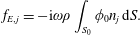 $$\begin{eqnarray}f_{E,j}=-\text{i}\unicode[STIX]{x1D714}\unicode[STIX]{x1D70C}\int _{S_{0}}\unicode[STIX]{x1D719}_{0}n_{j}\,\text{d}S.\end{eqnarray}$$
Substituting (3.71) together with (3.67) into (3.72), we have
 $$\begin{eqnarray}\displaystyle & \displaystyle f_{E,1}=-2\unicode[STIX]{x03C0}a\unicode[STIX]{x1D70C}\unicode[STIX]{x1D714}(A_{1}^{0}-B_{1}^{0}), & \displaystyle\end{eqnarray}$$
 $$\begin{eqnarray}\displaystyle & \displaystyle f_{E,2}=\text{i}2\unicode[STIX]{x03C0}a\unicode[STIX]{x1D70C}\unicode[STIX]{x1D714}(A_{1}^{0}+B_{1}^{0}). & \displaystyle\end{eqnarray}$$
We may notice that
 $f_{E,j}$
in (3.72) can be also computed through
 $\unicode[STIX]{x1D711}$
and
 $\unicode[STIX]{x1D719}_{j}$
by using the Haskind relation (C 5).
3.5 Some special cases
3.5.1 Simplified solution procedure at large
 $|x_{0}/a|$

When the circular cylinder is located far away from the crack, or
 $|x_{0}/a|\gg 1$
, the problems in §§ 3.3 and 3.4 can be solved by using the wide spacing approximation, based on the assumption that the mutual effects of evanescent waves between the crack and the body can be neglected. Without losing generality, here we may assume
 $x_{0}>0$
and the incoming wave is from
 $x=-\infty$
. We denote the radiation and scattering potentials of the body, with its centre at
 $x=0$
and submerged below the ice sheet without the crack, as
 $\unicode[STIX]{x1D713}_{j}^{r}$
and
 $\unicode[STIX]{x1D713}_{0}$
respectively. The solutions of these potentials can be obtained by dropping the terms of
 ${\mathcal{I}}_{1}$
and
 ${\mathcal{I}}_{2}$
in (3.43) and (3.44), and the procedure will be much simpler. We further define the velocity potentials
 $\unicode[STIX]{x1D713}_{L}$
and
 $\unicode[STIX]{x1D713}_{R}$
for ice sheet with a crack but without the body. They correspond to incoming waves from
 $x=-\infty$
and
 $x=+\infty$
respectively, and contain both the incident and diffracted potentials. These two potentials can be obtained directly from (3.62) and (3.66). Using these results the solution for the current problem of a body submerged beneath an ice sheet with a crack can be easily constructed for
 $|x_{0}/a|\gg 1$
, following the method used for multiple bodies with a large gap (Srokosz & Evans Reference Srokosz and Evans1979) and a floating body in a wide polynya (Li et al.
Reference Li, Shi and Wu2017a
).
We may notice that the transmission coefficient
 $T_{c}$
and reflection coefficient
 $R_{c}$
corresponding to
 $\unicode[STIX]{x1D713}_{L}$
and
 $\unicode[STIX]{x1D713}_{R}$
are the same, which can be easily confirmed through reversing the direction of the
 $x$
axis. At infinity, the evanescent waves will tend to zero and the velocity potentials defined above will have the following asymptotic forms
 $$\begin{eqnarray}\displaystyle & \displaystyle \unicode[STIX]{x1D713}_{j}^{r}=A_{j}^{\pm }\text{e}^{\mp \text{i}\unicode[STIX]{x1D706}x}\unicode[STIX]{x1D713}(z)\text{ as }x\rightarrow \pm \infty ,\quad (j=1,2), & \displaystyle\end{eqnarray}$$
 $$\begin{eqnarray}\displaystyle & \displaystyle \unicode[STIX]{x1D713}_{0}=t_{0}\text{e}^{-\text{i}\unicode[STIX]{x1D706}x}\unicode[STIX]{x1D713}(z)\text{ as }x\rightarrow +\infty , & \displaystyle\end{eqnarray}$$
 $$\begin{eqnarray}\displaystyle & \displaystyle \unicode[STIX]{x1D713}_{0}=(\text{e}^{-\text{i}\unicode[STIX]{x1D706}x}+r_{0}\text{e}^{+\text{i}\unicode[STIX]{x1D706}x})\unicode[STIX]{x1D713}(z)\text{ as }x\rightarrow -\infty , & \displaystyle\end{eqnarray}$$
 $$\begin{eqnarray}\displaystyle & \displaystyle \unicode[STIX]{x1D713}_{L}=T_{c}\text{e}^{-\text{i}\unicode[STIX]{x1D706}x}\unicode[STIX]{x1D713}(z)\text{ as }x\rightarrow +\infty , & \displaystyle\end{eqnarray}$$
 $$\begin{eqnarray}\displaystyle & \displaystyle \unicode[STIX]{x1D713}_{L}=(\text{e}^{-\text{i}\unicode[STIX]{x1D706}x}+R_{c}\text{e}^{+\text{i}\unicode[STIX]{x1D706}x})\unicode[STIX]{x1D713}(z)\text{ as }x\rightarrow -\infty , & \displaystyle\end{eqnarray}$$
 $$\begin{eqnarray}\displaystyle & \displaystyle \unicode[STIX]{x1D713}_{R}=(\text{e}^{+\text{i}\unicode[STIX]{x1D706}x}+R_{c}\text{e}^{-\text{i}\unicode[STIX]{x1D706}x})\unicode[STIX]{x1D713}(z)\text{ as }x\rightarrow +\infty , & \displaystyle\end{eqnarray}$$
 $$\begin{eqnarray}\displaystyle & \displaystyle \unicode[STIX]{x1D713}_{R}=T_{c}\text{e}^{+\text{i}\unicode[STIX]{x1D706}x}\unicode[STIX]{x1D713}(z)\text{ as }x\rightarrow -\infty . & \displaystyle\end{eqnarray}$$
 $j$
th mode, by following the procedure in Srokosz & Evans (Reference Srokosz and Evans1979), the velocity potential near the body can be written as a summation of the potential without a crack and the potential due to the wave reflected by the crack
 $$\begin{eqnarray}\unicode[STIX]{x1D719}_{j}(x,z)=\unicode[STIX]{x1D713}_{j}^{r}(x-x_{0},z)+\unicode[STIX]{x1D716}_{j}\unicode[STIX]{x1D713}_{0}(x-x_{0},z).\end{eqnarray}$$
Near the crack we may write the velocity potential as
 $$\begin{eqnarray}\unicode[STIX]{x1D719}_{j}(x,z)=\unicode[STIX]{x1D702}_{j}\unicode[STIX]{x1D713}_{R}(x,z),\end{eqnarray}$$
which is due to the incoming wave to the crack generated by the body motion and its reflection by the crack.
 $\unicode[STIX]{x1D716}_{j}$
and
 $\unicode[STIX]{x1D702}_{j}$
in the two equations are two unknown coefficients to be determined.
 $x-x_{0}$
in (3.76) reflects the fact that the solutions for
 $\unicode[STIX]{x1D713}_{j}^{r}$
and
 $\unicode[STIX]{x1D713}_{0}$
correspond to the cylinder with centre located at
 $(0,z_{0})$
, which in the current problem is at
 $(x_{0},z_{0})$
.
The solution has now been constructed based on results which could be obtained much more easily. The only task is to find the two unknown coefficients. We may consider (3.76) and (3.77) at a vertical line at
 $x=x_{I}$
between the crack and cylinder. On this vertical interface, the continuity conditions of pressure and normal velocity may be enforced, i.e.
 $$\begin{eqnarray}\unicode[STIX]{x1D719}_{j}(x_{I-},z)=\unicode[STIX]{x1D719}_{j}(x_{I+},z),\quad \frac{\unicode[STIX]{x2202}\unicode[STIX]{x1D719}_{j}(x_{I-},z)}{\unicode[STIX]{x2202}x}=\frac{\unicode[STIX]{x2202}\unicode[STIX]{x1D719}_{j}(x_{I+},z)}{\unicode[STIX]{x2202}x},\end{eqnarray}$$
where the subscripts
 $+$
and
 $-$
mean that the potentials should be taken from the solutions on the right- and left-hand sides of the vertical line, or (3.76) and (3.77), respectively. On the basis
 $0\ll x_{I}\ll x_{0}$
, (3.75a
)–(3.75g
) become applicable at
 $x=x_{I}$
. Substituting (3.76) and (3.77), and the corresponding asymptotic expansions into (3.78), we can obtain
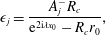 $$\begin{eqnarray}\displaystyle & \displaystyle \unicode[STIX]{x1D716}_{j}=\frac{A_{j}^{-}R_{c}}{\text{e}^{2\text{i}\unicode[STIX]{x1D706}x_{0}}-R_{c}r_{0}}, & \displaystyle\end{eqnarray}$$
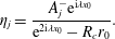 $$\begin{eqnarray}\displaystyle & \displaystyle \unicode[STIX]{x1D702}_{j}=\frac{A_{j}^{-}\text{e}^{\text{i}\unicode[STIX]{x1D706}x_{0}}}{\text{e}^{2\text{i}\unicode[STIX]{x1D706}x_{0}}-R_{c}r_{0}}. & \displaystyle\end{eqnarray}$$
Substituting (3.76) into (3.56), we can obtain the added mass and damping coefficient as
 $$\begin{eqnarray}\unicode[STIX]{x1D70F}_{js}=\unicode[STIX]{x1D70F}_{js}^{o}-\unicode[STIX]{x1D716}_{s}f_{E,j}^{o}/g,\end{eqnarray}$$
where the superscript
 $o$
means that the results are from the ice sheet without crack.
Similarly, for the diffraction problem, near the body we may write the potential as
 $$\begin{eqnarray}\unicode[STIX]{x1D719}_{0}(x,z)=\unicode[STIX]{x1D716}_{0}\unicode[STIX]{x1D713}_{0}(x-x_{0},z),\end{eqnarray}$$
and near the crack we may write the potential as
 $$\begin{eqnarray}\unicode[STIX]{x1D719}_{0}(x,z)=\unicode[STIX]{x1D713}_{L}(x,z)+\unicode[STIX]{x1D702}_{0}\unicode[STIX]{x1D713}_{R}(x,z).\end{eqnarray}$$
Using the asymptotic expansion and imposing the continuity condition (3.78) at
 $x=x_{I}$
, we have
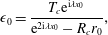 $$\begin{eqnarray}\displaystyle & \displaystyle \unicode[STIX]{x1D716}_{0}=\frac{T_{c}\text{e}^{\text{i}\unicode[STIX]{x1D706}x_{0}}}{\text{e}^{2\text{i}\unicode[STIX]{x1D706}x_{0}}-R_{c}r_{0}}, & \displaystyle\end{eqnarray}$$
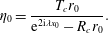 $$\begin{eqnarray}\displaystyle & \displaystyle \unicode[STIX]{x1D702}_{0}=\frac{T_{c}r_{0}}{\text{e}^{2\text{i}\unicode[STIX]{x1D706}x_{0}}-R_{c}r_{0}}. & \displaystyle\end{eqnarray}$$
Substituting (3.82) into (3.72), we can obtain the wave exciting force on the cylinder below the ice sheet with a crack from the result without the crack
 $$\begin{eqnarray}f_{E,j}=\unicode[STIX]{x1D716}_{0}f_{E,j}^{o}.\end{eqnarray}$$
We should notice that (3.81) and (3.86) are not limited to a circular cylinder and they are applicable for a body of arbitrary shape.
3.5.2 Solution for infinite water depth
When the water depth tends to infinity or
 $H\rightarrow +\infty$
,
 $G_{ice}$
and
 $G_{1}$
in the Green function (3.38) respectively become
 $$\begin{eqnarray}G_{ice}=\ln (r_{1})-\ln (r_{1}^{\prime })-2\int _{{\mathcal{D}}}\frac{Lk^{4}+\unicode[STIX]{x1D70C}g-m\unicode[STIX]{x1D714}^{2}}{K(\unicode[STIX]{x1D714},k)}\text{e}^{k(z+z_{0})}\cos [k(x-x_{0})]\,\text{d}k,\end{eqnarray}$$
and
 $$\begin{eqnarray}G_{1}=\frac{L}{\unicode[STIX]{x03C0}}\int _{{\mathcal{D}}}\frac{\text{e}^{kz}}{K(\unicode[STIX]{x1D714},k)}k^{2}\cos (kx)\,\text{d}k,\end{eqnarray}$$
together with
 ${\mathcal{I}}_{1}$
and
 ${\mathcal{I}}_{2}$
simplified as
 $$\begin{eqnarray}\displaystyle & \displaystyle {\mathcal{I}}_{1}=\int _{{\mathcal{D}}}\frac{\unicode[STIX]{x1D70C}\unicode[STIX]{x1D714}^{2}-(\unicode[STIX]{x1D70C}g-m\unicode[STIX]{x1D714}^{2})k}{K(\unicode[STIX]{x1D714},k)}k^{2}\,\text{d}k, & \displaystyle\end{eqnarray}$$
 $$\begin{eqnarray}\displaystyle & \displaystyle {\mathcal{I}}_{2}=\int _{{\mathcal{D}}}\frac{\unicode[STIX]{x1D70C}\unicode[STIX]{x1D714}^{2}-(\unicode[STIX]{x1D70C}g-m\unicode[STIX]{x1D714}^{2})k}{K(\unicode[STIX]{x1D714},k)}\,\text{d}k, & \displaystyle\end{eqnarray}$$
 $r_{1}^{\prime }$
is the distance between
 $p$
and the mirror image of
 $q$
about the mean upper surface
 $z=0$
, and
 $$\begin{eqnarray}K(\unicode[STIX]{x1D714},k)=(Lk^{4}+\unicode[STIX]{x1D70C}g-m\unicode[STIX]{x1D714}^{2})k-\unicode[STIX]{x1D70C}\unicode[STIX]{x1D714}^{2}.\end{eqnarray}$$
For the multipole expansions, (3.45a ) and (3.45b ) become
 $$\begin{eqnarray}\displaystyle & \displaystyle {\mathcal{G}}_{1}(n)=-2\int _{{\mathcal{D}}}\frac{\text{e}^{kz_{0}-\text{i}kx_{0}}}{K(\unicode[STIX]{x1D714},k)}k^{n+3}\,\text{d}k, & \displaystyle\end{eqnarray}$$
 $$\begin{eqnarray}\displaystyle & \displaystyle {\mathcal{G}}_{2}(n)=-2\int _{{\mathcal{D}}}\frac{\text{e}^{kz_{0}+\text{i}kx_{0}}}{K(\unicode[STIX]{x1D714},k)}k^{n+3}\,\text{d}k, & \displaystyle\end{eqnarray}$$
 $$\begin{eqnarray}\displaystyle & \displaystyle {\mathcal{J}}_{1}(n)=0, & \displaystyle\end{eqnarray}$$
 $$\begin{eqnarray}\displaystyle & \displaystyle {\mathcal{J}}_{2}(n)=0, & \displaystyle\end{eqnarray}$$
 $$\begin{eqnarray}\displaystyle & \displaystyle {\mathcal{J}}_{3}(n)=2\int _{{\mathcal{D}}}\left[1+\frac{2\unicode[STIX]{x1D70C}\unicode[STIX]{x1D714}^{2}}{K(\unicode[STIX]{x1D714},k)}\right]\text{e}^{2kz_{0}}k^{n-1}\,\text{d}k. & \displaystyle\end{eqnarray}$$
For the problem of wave propagation across the crack,
 ${\mathcal{F}}_{1}(n)$
and
 ${\mathcal{F}}_{2}(n)$
in (3.67) respectively become
 $$\begin{eqnarray}\displaystyle & \displaystyle {\mathcal{F}}_{1}(n)=-L\unicode[STIX]{x1D706}^{3}\left[\frac{\unicode[STIX]{x1D706}{\mathcal{G}}_{2}(n)}{{\mathcal{I}}_{1}}-\frac{{\mathcal{G}}_{2}(n-1)}{{\mathcal{I}}_{2}}\right], & \displaystyle\end{eqnarray}$$
 $$\begin{eqnarray}\displaystyle & \displaystyle {\mathcal{F}}_{2}(n)=4\unicode[STIX]{x1D706}^{4}\text{e}^{\unicode[STIX]{x1D706}z_{0}-\text{i}\unicode[STIX]{x1D706}x_{0}}+L\unicode[STIX]{x1D706}^{3}\left[\frac{\unicode[STIX]{x1D706}{\mathcal{G}}_{1}(n)}{{\mathcal{I}}_{1}}+\frac{{\mathcal{G}}_{1}(n-1)}{{\mathcal{I}}_{2}}\right]. & \displaystyle\end{eqnarray}$$
The simplified solution in § 3.5.1 can be also extended to infinite water depth. This is obtained by setting
 $\unicode[STIX]{x1D713}(z)$
in (3.75a–g
) as
 $\text{e}^{\unicode[STIX]{x1D706}z}$
, while the other equations remain the same.
When there is no ice crack, i.e. removing the terms
 ${\mathcal{I}}_{1}$
and
 ${\mathcal{I}}_{2}$
,
 ${\mathcal{F}}_{1}(n)$
in (3.93a
) and
 $E(n,l)$
in (3.50c
) become zero. Then (3.52) provides
 $A_{l}^{0}=0$
. By letting
 $H\rightarrow +\infty$
in (3.44), we obtain
 $\lim _{x\rightarrow -\infty }g_{n}=0$
. Thus according to (3.46), we can conclude that there is no wave reflection by the circular cylinder. If the ice thickness is taken to be zero, this becomes the well-known case for a free surface, as has been shown by Dean (Reference Dean1948) and Ursell (Reference Ursell1950). When the ice sheet has a crack, this conclusion is not true in general. However (3.91b
) provides
 $\lim _{x_{0}\rightarrow +\infty }{\mathcal{G}}_{2}(n)=0$
and we can also obtain
 $A_{l}^{0}=0$
. Thus there will be no reflection in such a case. This is of course quite obvious as the wave due to
 $\unicode[STIX]{x1D711}=\unicode[STIX]{x1D719}_{I}+\unicode[STIX]{x1D719}_{D}^{1}$
becomes the normal incident wave when
 $x_{0}\rightarrow +\infty$
, or the cylinder is infinitely far away from the crack.
4 Numerical results
The typical physical parameters of the ice sheet are chosen to be the same as those in Sturova (Reference Sturova2015b ), i.e.
 $$\begin{eqnarray}E=5~\text{Gpa},\quad \unicode[STIX]{x1D708}=0.3,\quad \unicode[STIX]{x1D70C}_{0}=922.5~\text{kg}\,\text{m}^{-3},\quad \unicode[STIX]{x1D70C}=1025~\text{kg}\,\text{m}^{-3},\quad H=100~\text{m}.\end{eqnarray}$$
Numerical results are obtained by truncating the infinite series of the multipole expansions at a finite number
 $n=N$
, and they are presented in the dimensionless form, based on a characteristic length scale, the density of water
 $\unicode[STIX]{x1D70C}$
and acceleration due to gravity
 $g=9.80~\text{m}~\text{s}^{-2}$
.
4.1 Wave scattering by an ice crack
We may use the problem of wave propagation beneath an ice sheet with a crack to first verify the present formulation. The case has been considered by Evans & Porter (Reference Evans and Porter2003). In that work, the problem was first divided into the symmetric and antisymmetric parts, and then Green’s identity was applied to each part together with the Green function satisfying the condition on the ice sheet without a crack. Thus the result for each part turned out to be a single series multiplied by an unknown constant which was further determined by the condition at the crack. Here, by taking the advantage of the Green function in (3.38), which itself already satisfies the ice crack condition, the solution can be obtained directly through the Green identity, as shown in (3.66). If we convert the integration in (3.66) into series form, it can be found that the solution is identical to that of Evans & Porter (Reference Evans and Porter2003). Taking
 $x\leqslant 0$
as an example, we first extend the route of integrations in (3.66) to
 $k\in (-\infty ,+\infty )$
, and add an integration along a semicircle of infinite radius in the lower half-complex plane of
 $k$
. The latter does not affect the result as it is in fact a zero term, which follows Jordan’s lemma. Then using residue theorem and noticing the poles at
 $-k_{n}$
,
 $n=-2,-1,0,1,\ldots$
in the lower half-plane, the potential
 $\unicode[STIX]{x1D711}$
can be expressed in the series form as
 $$\begin{eqnarray}\unicode[STIX]{x1D711}=\frac{I}{Z_{0}(0)}\unicode[STIX]{x1D711}_{0},\end{eqnarray}$$
where
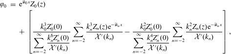 $$\begin{eqnarray}\displaystyle \unicode[STIX]{x1D711}_{0} & = & \displaystyle \text{e}^{\text{i}k_{0}x}Z_{0}(z)\nonumber\\ \displaystyle & & \displaystyle +\,\left[\frac{k_{0}^{3}Z_{0}^{\prime }(0)}{\displaystyle \mathop{\sum }_{n=-2}^{\infty }\frac{k_{n}^{6}Z_{n}^{\prime }(0)}{{\mathcal{X}}^{\prime }(k_{n})}}\mathop{\sum }_{n=-2}^{\infty }\frac{k_{n}^{3}Z_{n}(z)\text{e}^{-\text{i}k_{n}x}}{{\mathcal{X}}^{\prime }(k_{n})}-\frac{k_{0}^{2}Z_{0}^{\prime }(0)}{\displaystyle \mathop{\sum }_{n=-2}^{\infty }\frac{k_{n}^{4}Z_{n}^{\prime }(0)}{{\mathcal{X}}^{\prime }(k_{n})}}\mathop{\sum }_{n=-2}^{\infty }\frac{k_{n}^{2}Z_{n}(z)\text{e}^{-\text{i}k_{n}x}}{{\mathcal{X}}^{\prime }(k_{n})}\right],\qquad\end{eqnarray}$$
and
 $$\begin{eqnarray}\displaystyle & \displaystyle {\mathcal{X}}(k)=(L\unicode[STIX]{x1D706}^{4}+\unicode[STIX]{x1D70C}g-m\unicode[STIX]{x1D714}^{2})k\sinh (kH)-\unicode[STIX]{x1D70C}\unicode[STIX]{x1D714}^{2}\cosh (kH), & \displaystyle\end{eqnarray}$$
 $$\begin{eqnarray}\displaystyle & \displaystyle Z_{n}(z)=\cosh [k_{n}(z+H)]. & \displaystyle\end{eqnarray}$$
Here,
 $k_{0}=-\unicode[STIX]{x1D706}$
,
 $k_{n}$
with
 $n=1,2,\ldots$
are the purely positive imaginary roots of (2.8),
 $k_{-1}$
and
 $k_{-2}$
are the corresponding two complex roots with positive imaginary parts. It can be seen that (4.3) is identical to (2.17) in Evans & Porter (Reference Evans and Porter2003) for the normal incident case, by noticing that the time factor adopted by them is
 $\text{e}^{-\text{i}\unicode[STIX]{x1D714}t}$
, while
 $\text{e}^{+\text{i}\unicode[STIX]{x1D714}t}$
is used in (2.1) here.
At
 $x\rightarrow \pm \infty$
, by applying the Fourier integrals (13.16) in Wehausen & Laitone (Reference Wehausen and Laitone1960) to
 $\unicode[STIX]{x1D719}_{D}^{1}$
in (3.66), the potential
 $\unicode[STIX]{x1D711}$
can be given as
 $$\begin{eqnarray}\unicode[STIX]{x1D711}=\left\{\begin{array}{@{}ll@{}}\displaystyle I\times T_{c}\text{e}^{-\text{i}\unicode[STIX]{x1D706}x}\unicode[STIX]{x1D713}(z) & \text{at }x\rightarrow +\infty \\ \displaystyle I(\text{e}^{-\text{i}\unicode[STIX]{x1D706}x}+R_{c}\text{e}^{+\text{i}\unicode[STIX]{x1D706}x})\unicode[STIX]{x1D713}(z) & \text{at }x\rightarrow -\infty ,\end{array}\right.\end{eqnarray}$$
with transmission coefficient
 $T_{c}$
and reflection coefficient
 $R_{c}$
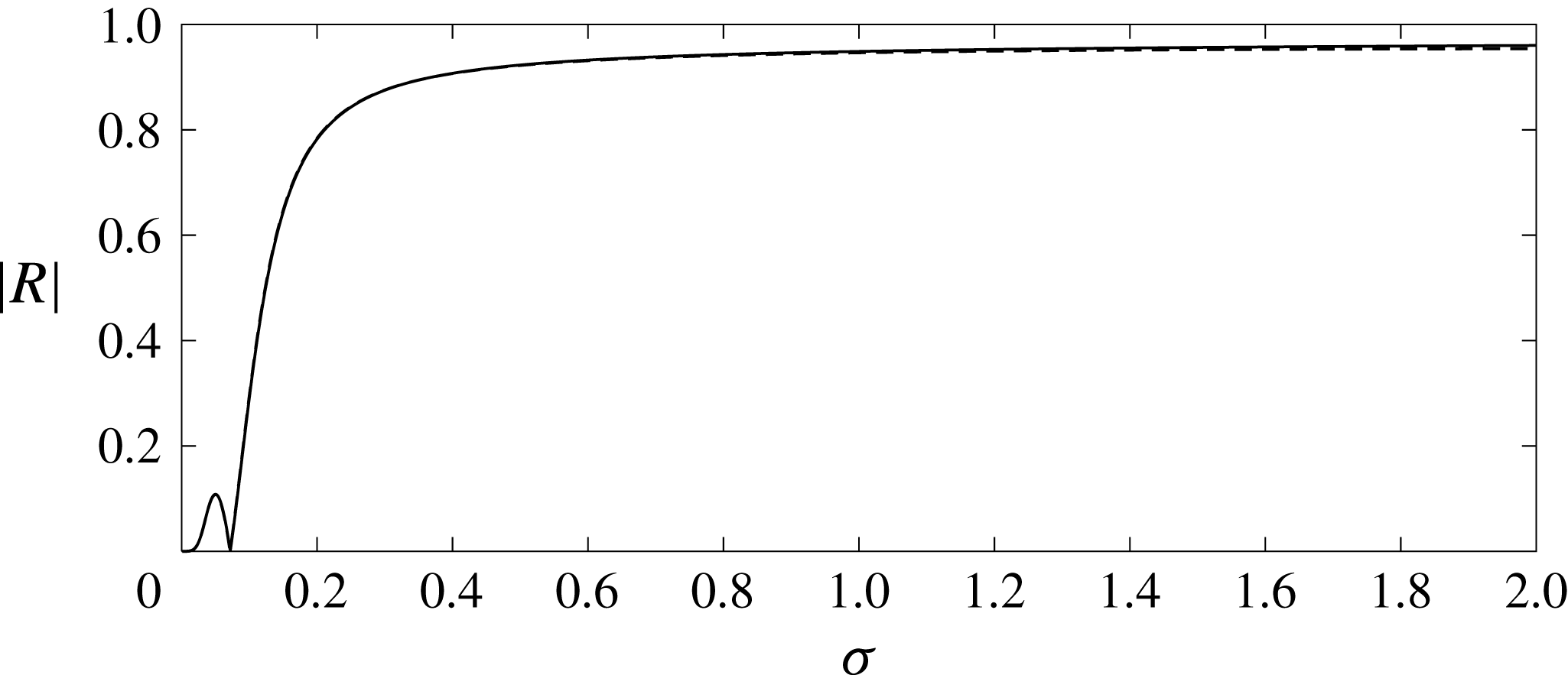
given in (B 7) and (B 8) respectively. It may be interesting to compare these results for wave propagation below an ice sheet with a crack and those through a polynya confined between two semi-infinite ice sheets. When the polynya width
 $b$
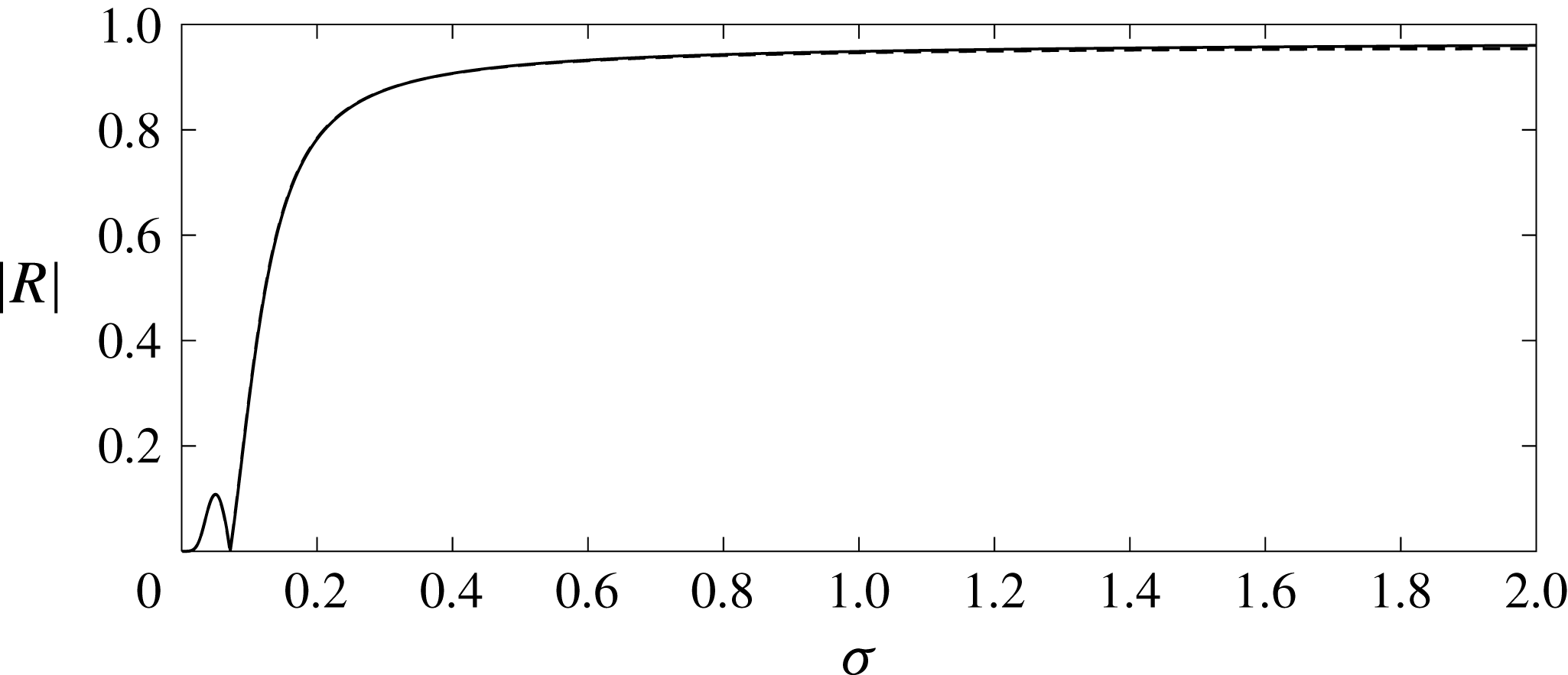
tends to zero, the result is expected to tend to that of an ice sheet with a crack. Comparison of the reflection coefficients is shown in figure 2, where
 $\unicode[STIX]{x1D70E}=\unicode[STIX]{x1D714}^{2}h/g$
, and
 $|R_{p}|$
for polynya with
 $b=0.05$
is computed by MEE (Ren et al.
Reference Ren, Wu and Thomas2016). From the figure, it can be seen that
 $|R_{p}|$
and
 $|R_{c}|$
agree with each other very well within the frequency range calculated.
Comparison of reflection coefficients. Solid line:
 $R_{c}$
for a crack; dashed line:
 $R_{p}$
for a polynya with
 $b=0.05$
. (
 $H=100$
,
 $h=1$
,
 $m=0.9$
,
 $L=45582$
.)
4.2 The radiation problem
We consider the radiation problem of a submerged circular cylinder, with its radius
 $a$
taken as the characteristic length. The convergence study with
 $N$
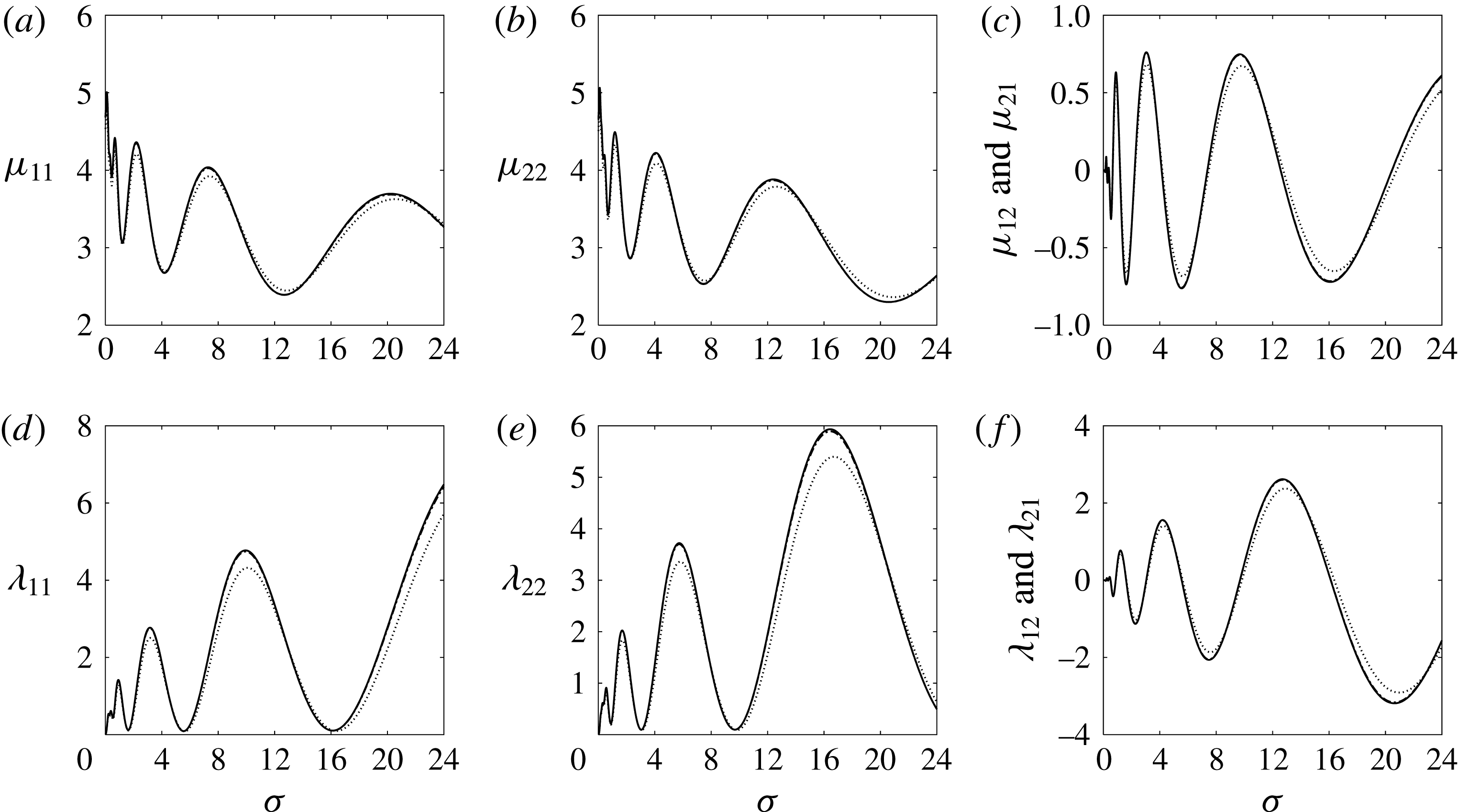
is first carried out through the hydrodynamic coefficients against
 $\unicode[STIX]{x1D70E}=\unicode[STIX]{x1D714}^{2}a/g$
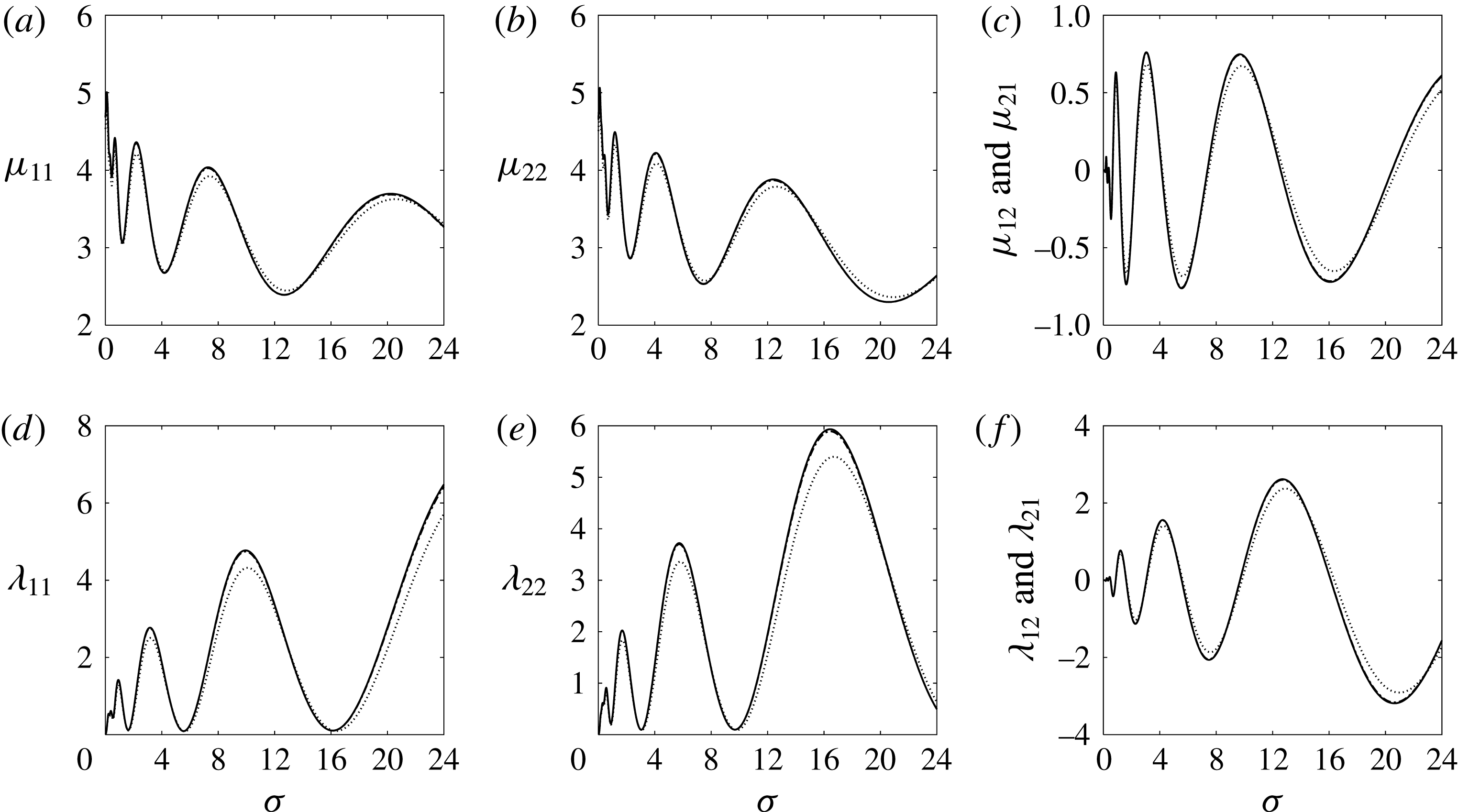
, as presented in figure 3. It can be seen that the numerical results converge very rapidly, and
 $N=5$
and
 $N=7$
give graphically indistinguishable results in the figure. The far field formula in the appendix has been used for calculating the damping coefficient and excellent agreement with the near field result has been found. For the results obtained subsequently we have taken
 $N=5$
.
Hydrodynamic coefficients of a submerged circular cylinder against
 $\unicode[STIX]{x1D70E}$
with different
 $N$
. Solid lines:
 $N=7$
; dashed lines:
 $N=5$
; dash-dotted lines:
 $N=3$
; dotted lines:
 $N=1$
. (
 $a=1$
,
 $x_{0}=20$
,
 $z_{0}=-1.2$
,
 $H=20$
,
 $h=0.2$
,
 $m=0.18$
,
 $L=72.932$
.)
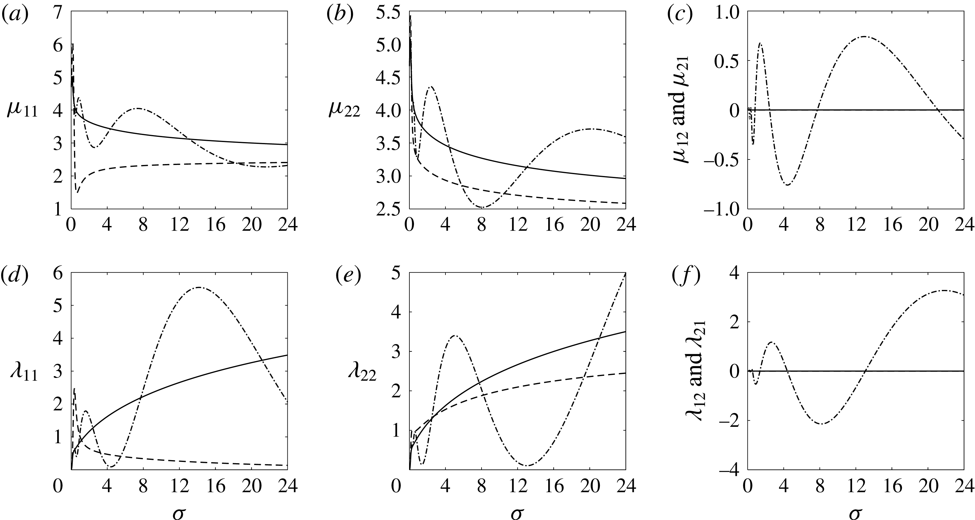
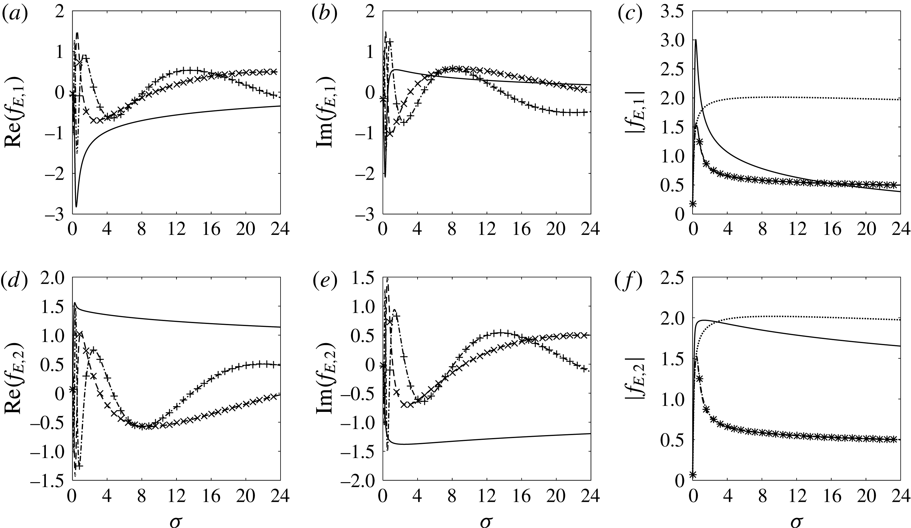
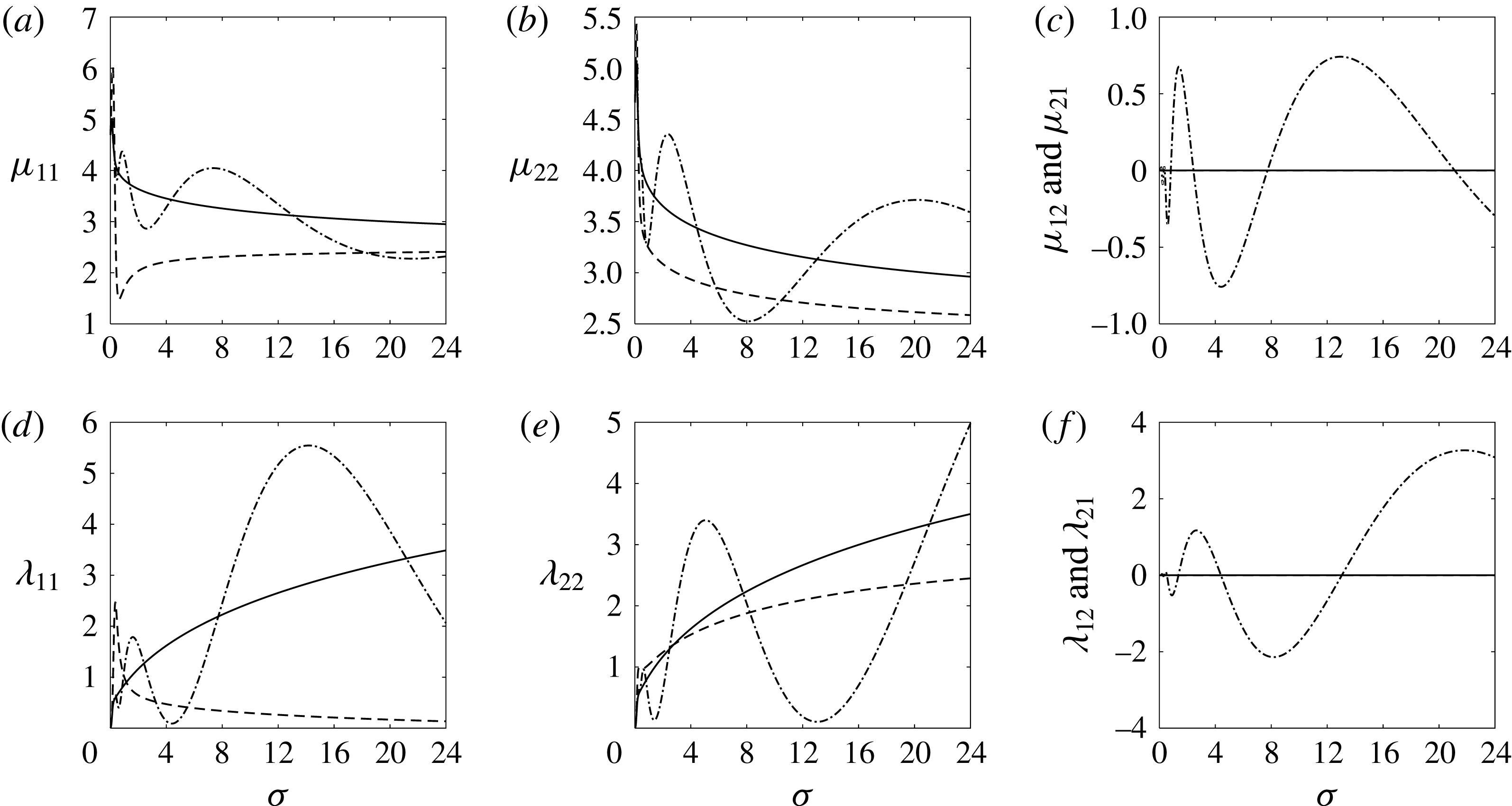
In figure 4 we show the hydrodynamic coefficients at different
 $x_{0}$
. As can be observed in this figure, when
 $\unicode[STIX]{x1D70E}\rightarrow 0$
, the results with the crack will tend to those without the crack. This is due to the fact that at very small
 $\unicode[STIX]{x1D70E}$
, the condition in (2.3) tends to
 $\unicode[STIX]{x2202}\unicode[STIX]{x1D719}_{j}/\unicode[STIX]{x2202}z=0$
on
 $z=0$
, which means
 $\unicode[STIX]{x2202}^{3}\unicode[STIX]{x1D719}_{j}/\unicode[STIX]{x2202}z\unicode[STIX]{x2202}x^{2}\rightarrow 0$
and
 $\unicode[STIX]{x2202}^{4}\unicode[STIX]{x1D719}_{j}/\unicode[STIX]{x2202}z\unicode[STIX]{x2202}x^{3}\rightarrow 0$
on the whole ice sheet. Therefore, the conditions at the crack will be automatically satisfied. Also as
 $\unicode[STIX]{x1D70E}\rightarrow 0$
, the effect of the position of
 $x_{0}$
diminishes. When
 $x_{0}=0$
, we have
 ${\mathcal{G}}_{1}(n)={\mathcal{G}}_{2}(n)$
in (3.45a
) and (3.45b
), which means in (3.50a
)–(3.50c
)
 $C(n,l)=C(l,n)$
and
 $D(n,l)=E(n,l)$
. Then (3.52) and (3.53) give
 $$\begin{eqnarray}A_{l}^{1}+B_{l}^{1}=0,\quad A_{l}^{2}-B_{l}^{2}=0.\end{eqnarray}$$
This suggests that
 $\unicode[STIX]{x1D719}_{1}$
and
 $\unicode[STIX]{x1D719}_{2}$
in (3.46) are antisymmetric and symmetric about the body centre respectively, as fully expected. Therefore, we have
 $\unicode[STIX]{x1D70F}_{js}$
equal to zero when
 $j\neq s$
.
Hydrodynamic coefficients of a submerged circular cylinder against
 $\unicode[STIX]{x1D70E}$
at different
 $x_{0}$
. Solid lines: ice sheet without crack; dashed lines:
 $x_{0}=0$
; dash-dotted lines:
 $x_{0}=10$
. (
 $a=1$
,
 $z_{0}=-1.2$
,
 $H=20$
,
 $h=0.2$
,
 $m=0.18$
,
 $L=72.932$
.)
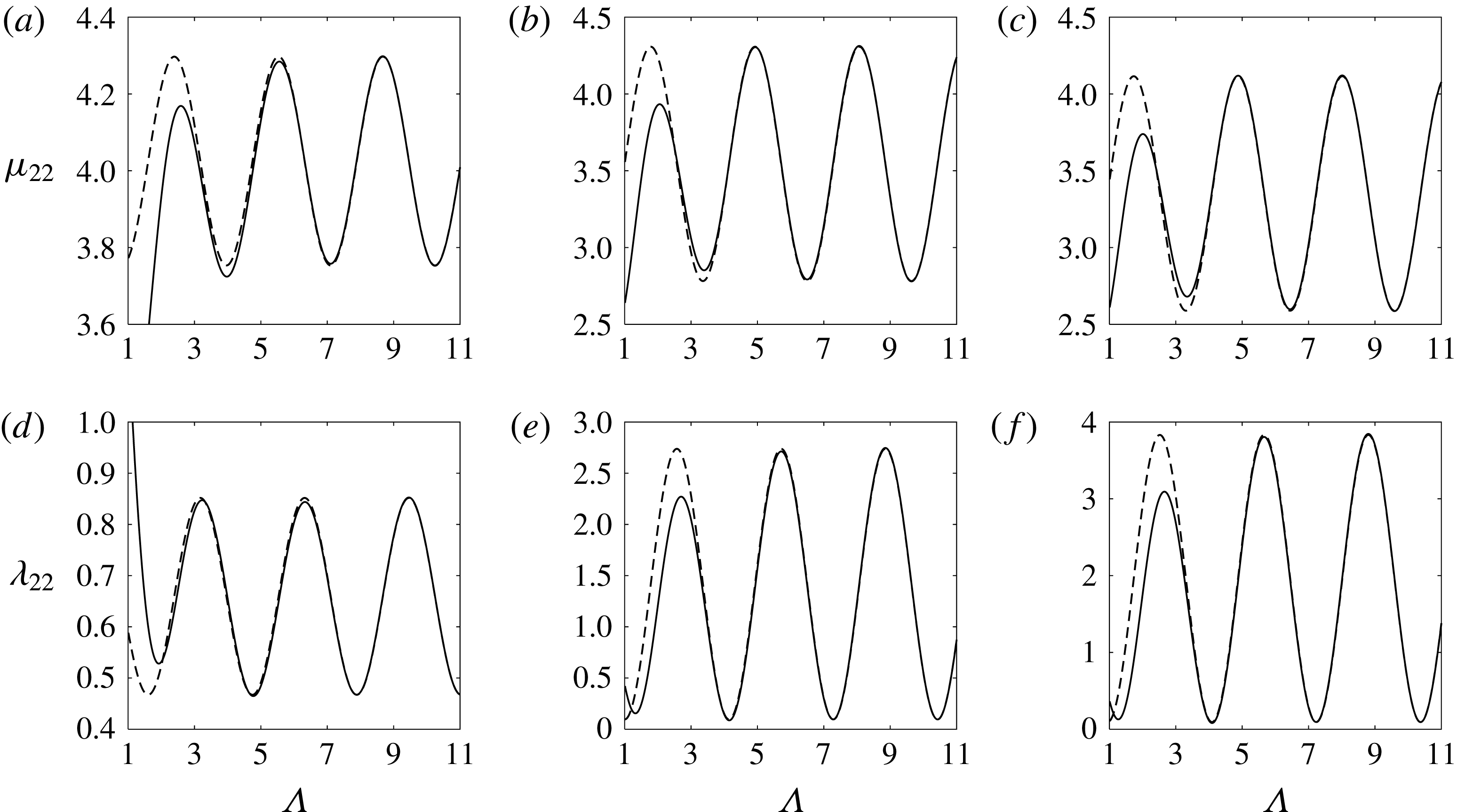
Hydrodynamic coefficients of a submerged circular cylinder against
 $\unicode[STIX]{x1D6EC}$
in heave mode. In (a) and (d),
 $\unicode[STIX]{x1D70E}=0.50$
; in (b) and (e),
 $\unicode[STIX]{x1D70E}=3.00$
; in (c) and (f),
 $\unicode[STIX]{x1D70E}=6.00$
. Solid line is for the exact results, while dashed line denotes the results from wide spacing approximation. (
 $a=1$
,
 $z_{0}=-1.2$
,
 $H=20$
,
 $h=0.2$
,
 $m=0.18$
,
 $L=72.932$
.)
We may notice in figure 4 that when
 $x_{0}\neq 0$
, the results are oscillatory with the frequency. Obviously, this is due to the fact that the wave generated by the body motion will arrive at the crack and then be reflected back to the body. This process is very much frequency dependent. Also we may infer that if we move the body position from
 $x_{0}$
to
 $x_{0}+\ell /2$
, where
 $\ell =2\unicode[STIX]{x03C0}/\unicode[STIX]{x1D706}$
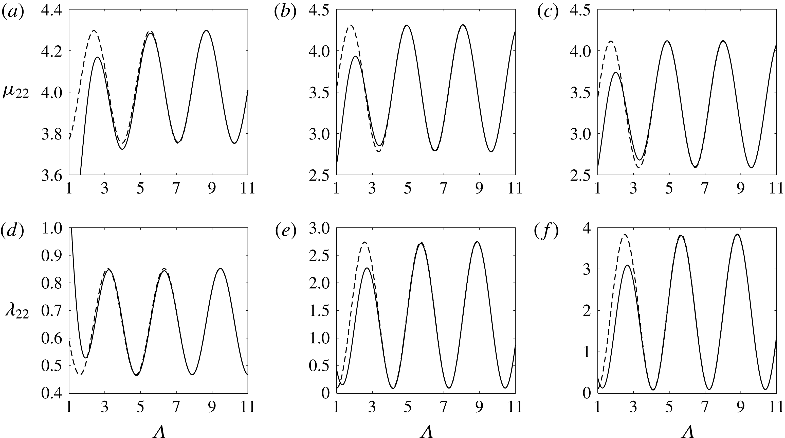
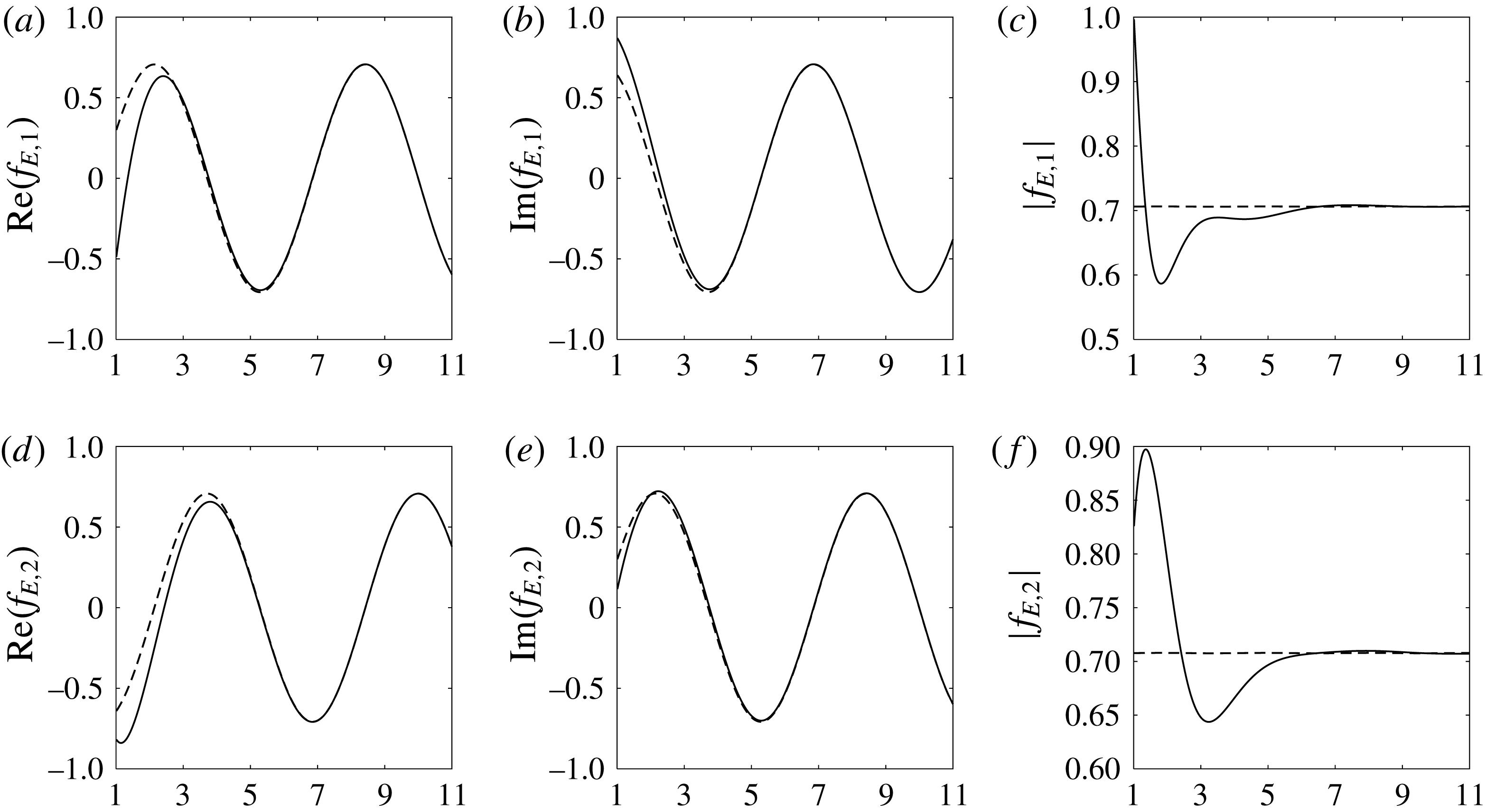
is the wavelength of the travelling wave generated by the body, the effect of the crack may be almost the same. To verify that, in figure 5 we plot
 $\unicode[STIX]{x1D707}_{22}$
and
 $\unicode[STIX]{x1D706}_{22}$
against
 $\unicode[STIX]{x1D6EC}=\unicode[STIX]{x1D706}x_{0}$
at various
 $\unicode[STIX]{x1D70E}$
, or a fixed
 $\unicode[STIX]{x1D706}$
when
 $x_{0}$
varies. It can be seen that the results become virtually periodic with
 $x_{0}$
when
 $\unicode[STIX]{x1D6EC}>4$
and they also become graphically indistinguishable to those from wide approximation method. To provide further insight into what has been observed in figure 5, we may follow the procedure in Li et al. (Reference Li, Shi and Wu2017a
) and use the equations in § 3.5.1.
Similar to (B 4),
 $f_{E,j}^{o}$
for the ice sheet without the crack can be expressed through the far field formula as
 $$\begin{eqnarray}f_{E,j}^{o}=2I\unicode[STIX]{x1D70C}\unicode[STIX]{x1D714}Q_{0}C_{g}A_{j}^{-},\end{eqnarray}$$
where
 $Q_{0}$
and
 $C_{g}$
are given in (A 7) and (A 8) respectively. Then invoking (3.81), we have
 $$\begin{eqnarray}\unicode[STIX]{x1D70F}_{js}=\unicode[STIX]{x1D70F}_{js}^{o}+2\text{i}\unicode[STIX]{x1D70C}Q_{0}C_{g}A_{js},\end{eqnarray}$$
where
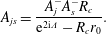 $$\begin{eqnarray}A_{js}=\frac{A_{j}^{-}A_{s}^{-}R_{c}}{\text{e}^{2\text{i}\unicode[STIX]{x1D6EC}}-R_{c}r_{0}}.\end{eqnarray}$$
For a given
 $\unicode[STIX]{x1D70E}$
, (4.10) shows that
 $A_{js}$
is periodic against
 $x_{0}$
with period of
 $\ell /2$
. This means that
 $\unicode[STIX]{x1D707}_{js}$
and
 $\unicode[STIX]{x1D706}_{js}$
both will respectively have the same values at
 $x_{0}+n\ell /2$
, where
 $n$
includes all integers to ensure that
 $x_{0}$
is positive. From (4.10) it can be also seen that
 $A_{js}$
maps the unit circle
 $\text{e}^{2\text{i}\unicode[STIX]{x1D6EC}}$
to a circle with centre at
 $$\begin{eqnarray}y_{c,r}=x_{c,r}+\text{i}z_{c,r}=-|R_{c}r_{0}|r_{r}\text{e}^{\text{i}\unicode[STIX]{x1D717}_{r}},\end{eqnarray}$$
and radius as
 $$\begin{eqnarray}r_{r}=\frac{|A_{j}^{-}A_{s}^{-}R_{c}|}{1-|R_{c}r_{0}|^{2}},\end{eqnarray}$$
where
 $$\begin{eqnarray}\text{e}^{\text{i}\unicode[STIX]{x1D717}_{r}}=\frac{A_{j}^{-}A_{s}^{-}\bar{r_{0}}}{|A_{j}^{-}A_{s}^{-}\bar{r_{0}}|}.\end{eqnarray}$$
From (4.11) and (4.12), (4.10) can be rewritten as
 $$\begin{eqnarray}A_{js}=y_{c,r}+r_{r}\text{e}^{\text{i}\unicode[STIX]{x1D70F}_{r}}.\end{eqnarray}$$
This indicates that the peak (
 $+$
) and trough (
 $-$
) of
 $\unicode[STIX]{x1D707}_{js}$
respectively equal
 $$\begin{eqnarray}\unicode[STIX]{x1D707}_{js}^{\pm }=\unicode[STIX]{x1D707}_{js}^{o}-2\unicode[STIX]{x1D70C}Q_{0}C_{g}(z_{c,r}\mp r_{r}),\end{eqnarray}$$
and they occur respectively when
 $\unicode[STIX]{x1D70F}_{r}$
equals
 $-\unicode[STIX]{x03C0}/2$
or
 $\unicode[STIX]{x03C0}/2$
. Similarly, the peak (
 $+$
) and trough (
 $-$
) of
 $\unicode[STIX]{x1D706}_{js}$
respectively equal
 $$\begin{eqnarray}\unicode[STIX]{x1D706}_{js}^{\pm }=\unicode[STIX]{x1D706}_{js}^{o}-2\unicode[STIX]{x1D714}\unicode[STIX]{x1D70C}Q_{0}C_{g}(x_{c,r}\mp r_{r}),\end{eqnarray}$$
and they occur respectively when
 $\unicode[STIX]{x1D70F}_{r}$
equals
 $\unicode[STIX]{x03C0}$
or
 $0$
. We may notice that the corresponding
 $\unicode[STIX]{x1D6EC}$
for
 $\unicode[STIX]{x1D707}_{js}^{\pm }$
and
 $\unicode[STIX]{x1D706}_{js}^{\pm }$
can be further obtained from (4.10) and (4.14).
The above discussions are valid for a body of general shape. For the circular cylinder, (4.10) may be further simplified. As shown in § 3.5.2,
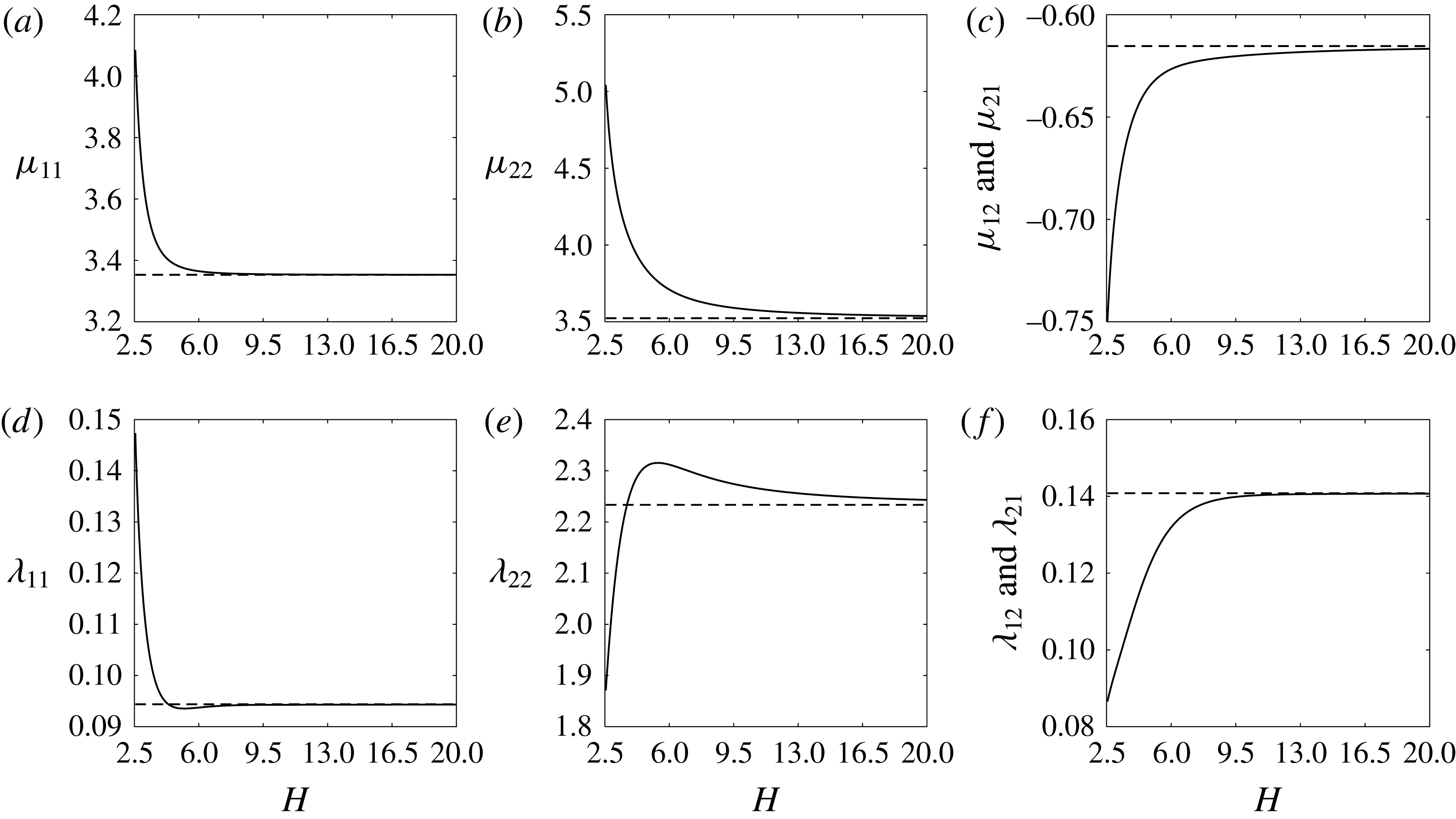
 $|r_{0}|$
is zero for infinite water depth. For the finite water depth neither
 $\unicode[STIX]{x1D707}_{l}(0)$
nor
 $E(n,l)$
is zero, and
 $|r_{0}|$
will not exactly be zero. However,
 $|r_{0}|$
is still much smaller than
 $|t_{0}|$
. In fact it has been found that
 $|r_{0}|<0.01$
over the range of
 $\unicode[STIX]{x1D70E}$
in figures 4 and 5. Thus (4.10) can be approximated as
 $$\begin{eqnarray}A_{js}\approx A_{j}^{-}A_{s}^{-}R_{c}\text{e}^{-2\text{i}\unicode[STIX]{x1D6EC}},\end{eqnarray}$$
which gives
 $y_{c,r}\approx 0$
and
 $r_{r}\approx |A_{j}^{-}A_{s}^{-}R_{c}|$
. These indicate that the local extrema of
 $\unicode[STIX]{x1D707}_{js}$
and
 $\unicode[STIX]{x1D706}_{js}$
will appear when
 $A_{js}$
respectively becomes a purely imaginary or real number, and if one of them reaches a local extremum, the other will reach the value for ice sheet without the crack.
Hydrodynamic coefficients of a submerged circular cylinder against
 $H$
. Solid line represents the results by the method for finite water depth, while dashed line represents those by the method for infinite water depth. (
 $a=1$
,
 $(x_{0},z_{0})=(5.0,-1.2)$
,
 $\unicode[STIX]{x1D70E}=3.00$
,
 $h=0.2$
,
 $m=0.18$
,
 $L=72.932$
.)
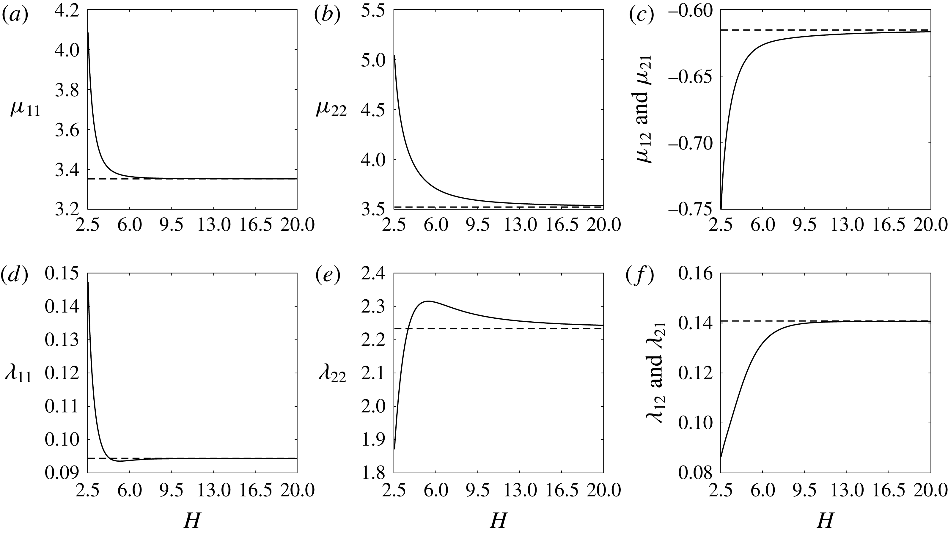
In figure 6, we show the hydrodynamic coefficients against
 $H$
for a given
 $\unicode[STIX]{x1D70E}$
. As can be expected, the results tend to those for infinite water depth as
 $H$
becomes larger. However for the heave mode, or
 $j=2$
, it can be seen that this trend is very slow.
For the problem of a free surface with infinite water depth, Ogilvie (Reference Ogilvie1963) found that the wave generated by the forced body oscillation would propagate only in one direction if the path of the circular cylinder centre follows a circular orbit. When the water surface is covered by an ice sheet, a similar conclusion may be drawn. Removing the terms related to
 ${\mathcal{I}}_{1}$
and
 ${\mathcal{I}}_{2}$
in (3.50a
)–(3.50c
) and noticing (3.92a
)–(3.92c
), invoking (3.52) we have
 $$\begin{eqnarray}A_{l}^{2}=\text{i}A_{l}^{1}.\end{eqnarray}$$
We may take the clockwise rotation as an example. This is achieved by taking the motion amplitudes
 $|\unicode[STIX]{x1D6FC}_{1}|=|\unicode[STIX]{x1D6FC}_{2}|$
in (2.1), and their phases
 $\unicode[STIX]{x1D717}_{2}=\unicode[STIX]{x1D717}_{1}+\unicode[STIX]{x03C0}/2$
. Invoking (3.46) and (4.18) we obtain
 $$\begin{eqnarray}\unicode[STIX]{x1D6F7}(x,z,t)=\text{Re}\left[\text{i}\unicode[STIX]{x1D714}\text{e}^{\text{i}\unicode[STIX]{x1D714}t}\unicode[STIX]{x1D6FC}_{1}\mathop{\sum }_{n=1}^{\infty }a^{n}(B_{n}^{1}\text{e}^{\text{i}\unicode[STIX]{x1D717}_{1}}+\text{i}B_{n}^{2}\text{e}^{\text{i}\unicode[STIX]{x1D717}_{1}})g_{n}\right].\end{eqnarray}$$
Since
 $\lim _{x\rightarrow -\infty }g_{n}=0$
, we can conclude that clockwise oscillation will generate the wave propagating to
 $x=+\infty$
only. Similarly, the counterclockwise oscillation will generate the wave propagating to
 $x=-\infty$
only due to
 $\lim _{x\rightarrow +\infty }f_{n}=0$
. When there is a crack in the ice sheet, since the equations for
 $A_{l}^{j}$
and
 $B_{l}^{j}$
are coupled, (4.18) is not valid in general. However, when
 $x_{0}\rightarrow +\infty$
, we have
 ${\mathcal{G}}_{2}(n)\rightarrow 0$
in (3.91b
), which gives
 $E(n,l)\rightarrow 0$
in (3.50c
). Substituting this into (3.52), we can obtain (4.18) again, i.e. no wave will propagate to
 $x=-\infty$
for clockwise oscillation.
Wave exciting force on a submerged circular cylinder against
 $\unicode[STIX]{x1D70E}$
at different
 $x_{0}$
. Solid lines:
 $x_{0}=0$
; dashed lines:
 $x_{0}=10$
; dash-dotted lines:
 $x_{0}=20$
; dotted lines: ice sheet without crack.
 $\times$
and
 $+$
are the wide spacing solutions for
 $x_{0}=10$
and
 $x_{0}=20$
, respectively. (
 $a=1$
,
 $z_{0}=-1.2$
,
 $H=20$
,
 $h=0.2$
,
 $m=0.18$
,
 $L=72.932$
.)
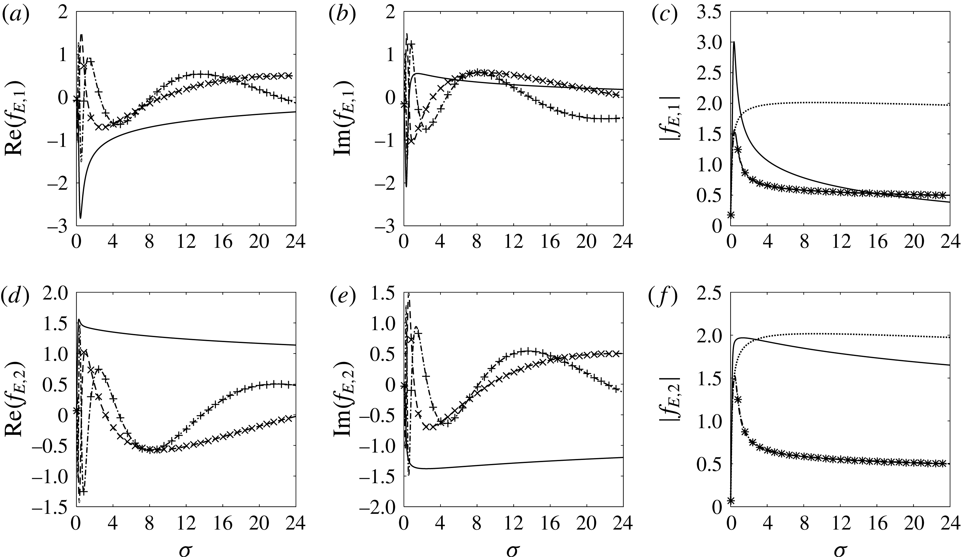
4.3 The diffraction problem
We then consider the problem of wave diffraction by the submerged circular cylinder. Figure 7 presents the results for the excitation force at different
 $x_{0}$
against
 $\unicode[STIX]{x1D70E}$
, together with those for the ice sheet without crack. From each figure, it can be seen that the results tend to the same value when
 $\unicode[STIX]{x1D70E}\rightarrow 0$
, for the reason discussed in § 4.2. It can also be seen that when
 $x_{0}$
is sufficiently large, the exact results are hardly different from those from the wide spacing method in § 3.5.1, even for very long waves, although the approximation is based on the assumption that
 $x_{0}$
is much larger than the wavelength. The reason for that is when
 $\unicode[STIX]{x1D70E}\rightarrow 0$
,
 $\unicode[STIX]{x1D716}_{0}\rightarrow 1$
. Then invoking (3.86) we have that
 $f_{E,j}$
tends to
 $f_{E,j}^{o}$
, or it tends to the exact result. This reveals that the wide spacing approximation can work well for both small and large
 $\unicode[STIX]{x1D70E}$
.
We may use the wide spacing approximation in (3.86) to give some insights into the features of the wave exciting force. Substituting (3.84) into (3.86) and invoking (4.8), we obtain
 $$\begin{eqnarray}f_{E,j}=-2\text{i}\unicode[STIX]{x1D70C}gQ_{0}C_{g}(A_{j}^{-}\unicode[STIX]{x1D716}_{0}\text{e}^{\text{i}\unicode[STIX]{x1D6EC}})\text{e}^{-\text{i}\unicode[STIX]{x1D6EC}}.\end{eqnarray}$$
Here
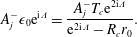 $$\begin{eqnarray}A_{j}^{-}\unicode[STIX]{x1D716}_{0}\text{e}^{\text{i}\unicode[STIX]{x1D6EC}}=\frac{A_{j}^{-}T_{c}\text{e}^{2\text{i}\unicode[STIX]{x1D6EC}}}{\text{e}^{2\text{i}\unicode[STIX]{x1D6EC}}-R_{c}r_{0}}.\end{eqnarray}$$
It should be noticed that the oscillatory term
 $A_{j}^{-}\unicode[STIX]{x1D716}_{0}\text{e}^{\text{i}\unicode[STIX]{x1D6EC}}$
is due to the interaction between the cylinder and the crack, while the oscillatory term
 $\text{e}^{-\text{i}\unicode[STIX]{x1D6EC}}$
is due to the initial phase of the incident potential
 $\unicode[STIX]{x1D719}_{I}$
relative to the body at
 $x_{0}$
. From (4.20), we can see that at a fixed
 $\unicode[STIX]{x1D70E}$
,
 $f_{E,j}$
is periodic against
 $\unicode[STIX]{x1D6EC}$
or it varies periodically with
 $x_{0}$
. The period for
 $\text{Re}(f_{E,j})$
and
 $\text{Im}(f_{E,j})$
equals
 $2\unicode[STIX]{x03C0}$
, as can be observed in figure 8.
Wave exciting force on a submerged circular cylinder against
 $\unicode[STIX]{x1D6EC}$
. Solid line is for the exact results, while dashed line denotes the results from wide spacing approximation. (
 $a=1$
,
 $z_{0}=-1.2$
,
 $\unicode[STIX]{x1D70E}=3.00$
,
 $H=20$
,
 $h=0.2$
,
 $m=0.18$
,
 $L=72.932$
.)
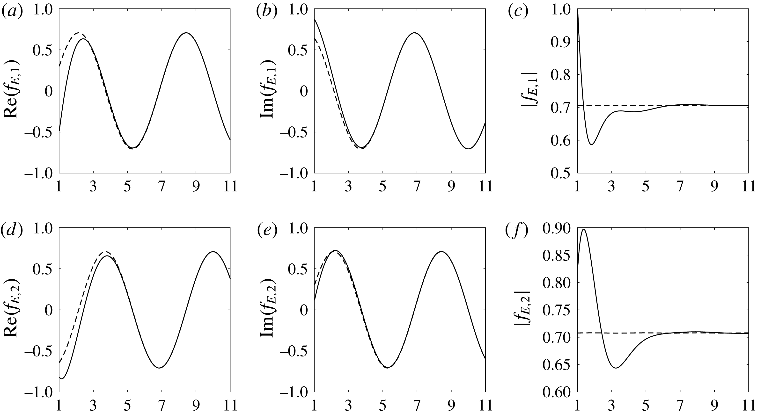
From (4.21) it can be seen that
 $A_{j}^{-}\unicode[STIX]{x1D716}_{0}\text{e}^{\text{i}\unicode[STIX]{x1D6EC}}$
maps the unit circle
 $\text{e}^{2\text{i}\unicode[STIX]{x1D6EC}}$
to a circle with centre at
 $$\begin{eqnarray}y_{c,d}=x_{c,d}+\text{i}z_{c,d}=\frac{|1-2|R_{c}r_{0}|^{2}|}{|R_{c}r_{0}|}r_{d}\text{e}^{\text{i}\unicode[STIX]{x1D717}_{d}},\end{eqnarray}$$
and radius as
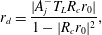 $$\begin{eqnarray}r_{d}=\frac{|A_{j}^{-}T_{L}R_{c}r_{0}|}{1-|R_{c}r_{0}|^{2}},\end{eqnarray}$$
where
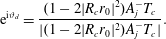 $$\begin{eqnarray}\text{e}^{\text{i}\unicode[STIX]{x1D717}_{d}}=\frac{(1-2|R_{c}r_{0}|^{2})A_{j}^{-}T_{c}}{|(1-2|R_{c}r_{0}|^{2})A_{j}^{-}T_{c}|}.\end{eqnarray}$$
From (4.22) and (4.23), (4.21) can be rewritten as
 $$\begin{eqnarray}A_{j}^{-}\unicode[STIX]{x1D716}_{0}\text{e}^{\text{i}\unicode[STIX]{x1D6EC}}=y_{c,d}+r_{d}\text{e}^{\text{i}\unicode[STIX]{x1D70F}_{d}}.\end{eqnarray}$$
This indicates that the peak (
 $+$
) and trough (
 $-$
) of
 $|f_{E,j}|$
respectively equal
 $$\begin{eqnarray}|f_{E,j}^{\pm }|=2\unicode[STIX]{x1D70C}gQ_{0}C_{g}||y_{c,d}|\pm r_{d}|,\end{eqnarray}$$
and they occur respectively when
 $\unicode[STIX]{x1D70F}_{d}$
equals
 $\unicode[STIX]{x1D717}_{d}$
or
 $\unicode[STIX]{x1D717}_{d}+\unicode[STIX]{x03C0}$
, and the corresponding
 $\unicode[STIX]{x1D6EC}$
can be further obtained according to (4.21) and (4.25). For the special case
 $1-2|R_{c}r_{0}|^{2}=0$
, we have
 $y_{c,d}=0$
and
 $|f_{E,j}^{+}|=|f_{E,j}^{-}|$
, which means that the location of the cylinder no longer has an effect on the magnitude of the force and the magnitude of the force is no longer oscillatory with respect to
 $x_{0}$
.
We may notice that the above discussions are valid for a body of generalized shape. For the present case of a circular cylinder, we may use the fact that
 $r_{0}\approx 0$
. Equation (4.21) becomes
 $$\begin{eqnarray}A_{j}^{-}\unicode[STIX]{x1D716}_{0}\text{e}^{\text{i}\unicode[STIX]{x1D6EC}}\approx A_{j}^{-}T_{c}.\end{eqnarray}$$
Substituting (4.27) into (4.20), it can be found that the oscillations of
 $\text{Re}(f_{E,j})$
and
 $\text{Im}(f_{E,j})$
in figure 8 are purely due to the fact that the cylinder is placed at a different horizontal position which causes the relative phase change of the incident wave. The magnitude of the exciting force becomes
 $|f_{E,j}|=2\unicode[STIX]{x1D70C}gQ_{0}C_{g}|A_{j}^{-}T_{c}|$
, which is not affected by
 $x_{0}$
, as can be seen in figure 8. We may notice that although
 $|f_{E,j}|$
tends to a constant as
 $x_{0}$
increases, the value of the constant is different from the force on the body without a crack. This is because
 $\unicode[STIX]{x1D719}_{D}^{1}$
in (3.61) at the body does not tend to zero even when
 $x_{0}\rightarrow +\infty$
. In fact, we have
 $|f_{E,j}|<|f_{E,j}^{o}|$
because
 $|T_{c}|<1$
is always valid based on the energy conservation equation (Barrett & Squire Reference Barrett and Squire1996).
5 Conclusions
The solution for the wave radiation and diffraction by a circular cylinder submerged below an ice sheet with a crack has been presented. The Green function satisfying both the ice sheet and the crack conditions is obtained in an integral form. By using this Green function, the solution for the problem of wave diffraction by the crack in the absence of the body is solved directly. The solution for each multipole is derived directly from the differentiation of the Green function with respect to the source position, from which the velocity potential for a submerged circular cylinder is constructed.
For the solution of wave diffraction by a polynya, results show that the reflection coefficient tends to that of a crack when the polynya width tends to zero. The hydrodynamic coefficients and exciting force of a submerged cylinder are found to be quite oscillatory with the frequency when the body is not right below the crack. However, the oscillation of the exciting force is observed only in its real and imaginary parts separately and there is no strong oscillation in the magnitude of the force. When the cylinder is away from the crack, accurate solution can be obtained through the wide spacing approximation method. From this method, it is shown explicitly that at a given frequency, the hydrodynamic coefficients, and the real and imaginary parts of the exciting force vary periodically with the distance between the cylinder and crack. This means that the effect of the crack always exists even when the distance tends to infinity. It can therefore be expected that the motion amplitude of the body will be quite oscillatory with the wave frequency and with the location of the crack, as in the case of polynya (Li et al. Reference Li, Shi and Wu2018), which has important implications for the performance of a marine vehicle in ice covered waters.
The Green function derived in this work also has much wider applications apart from being used as the starting point for the multipole expansion in the paper. Its simple form allows the function to be evaluated efficiently, instead of through solving a large matrix equation obtained from truncations of infinite series repeatedly for the source at each different position, as done in the previous work. The derived Green function allows the traditional method of source distribution over the body surface in the free surface flow problem to be used directly for a body submerged below an ice sheet with a crack. This makes the simulation for a cross-section of a realistic ship possible.
The solution procedure can be further extended to other forms of crack conditions, e.g. hinged or connected by springs, which may have practical implications in wave power absorptions or hydroelasticities. The solution procedure can be also used as a base for the derivation of a solution for an ice sheet with multiple cracks. However, the method is limited to the case in which the physical properties of the ice sheet are constant. It should be also mentioned that the analysis is within the scope of the linear velocity potential theory, which is not valid when the incoming wave amplitude or the body motion amplitude is large compared with the wavelength or the body dimension.
Acknowledgements
This work is supported by Lloyd’s Register Foundation through the joint centre involving University College London, Shanghai Jiaotong University and Harbin Engineering University, to which the authors are most grateful. Lloyd’s Register Foundation helps to protect life and property by supporting engineering-related education, public engagement, and the application of research. This work is also supported by the National Natural Science Foundation of China (grant nos 11472088 and 51709131).
Appendix A. The far field formula for the damping coefficient
From (3.56), we have
 $$\begin{eqnarray}\unicode[STIX]{x1D70F}_{js}-\unicode[STIX]{x1D70F}_{sj}=\unicode[STIX]{x1D70C}\int _{S_{0}}\left(\unicode[STIX]{x1D719}_{s}\frac{\unicode[STIX]{x2202}\unicode[STIX]{x1D719}_{j}}{\unicode[STIX]{x2202}n}-\unicode[STIX]{x1D719}_{j}\frac{\unicode[STIX]{x2202}\unicode[STIX]{x1D719}_{s}}{\unicode[STIX]{x2202}n}\right)\,\text{d}S.\end{eqnarray}$$
The integral over the body surface
 $S_{0}$
can be converted into the rest of the fluid boundary through Green’s identity. By using the corresponding boundary conditions, we can obtain
 $\unicode[STIX]{x1D70F}_{js}-\unicode[STIX]{x1D70F}_{sj}=0$
, or
 $$\begin{eqnarray}\unicode[STIX]{x1D707}_{js}=\unicode[STIX]{x1D707}_{sj},\quad \unicode[STIX]{x1D706}_{js}=\unicode[STIX]{x1D706}_{sj}.\end{eqnarray}$$
For the damping coefficient
 $\unicode[STIX]{x1D706}_{js}$
, (3.56) gives
 $$\begin{eqnarray}-\frac{2\text{i}}{\unicode[STIX]{x1D714}}\unicode[STIX]{x1D706}_{js}=\unicode[STIX]{x1D70C}\int _{S_{0}}\left(\unicode[STIX]{x1D719}_{s}\frac{\unicode[STIX]{x2202}\bar{\unicode[STIX]{x1D719}_{j}}}{\unicode[STIX]{x2202}n}-\bar{\unicode[STIX]{x1D719}_{j}}\frac{\unicode[STIX]{x2202}\unicode[STIX]{x1D719}_{s}}{\unicode[STIX]{x2202}n}\right)\,\text{d}S,\end{eqnarray}$$
where the overbar means conjugation. This integral can be converted to the rest of the fluid boundary and it will become
 $$\begin{eqnarray}\displaystyle & & \displaystyle -\frac{2\text{i}}{\unicode[STIX]{x1D714}}\unicode[STIX]{x1D706}_{js}=-\unicode[STIX]{x1D70C}\int _{S_{+\infty }+S_{-\infty }}\left(\unicode[STIX]{x1D719}_{s}\frac{\unicode[STIX]{x2202}\bar{\unicode[STIX]{x1D719}_{j}}}{\unicode[STIX]{x2202}n}-\bar{\unicode[STIX]{x1D719}_{j}}\frac{\unicode[STIX]{x2202}\unicode[STIX]{x1D719}_{s}}{\unicode[STIX]{x2202}n}\right)\,\text{d}S\nonumber\\ \displaystyle & & \displaystyle \quad -\,\frac{L}{\unicode[STIX]{x1D714}^{2}}\left[\left(\frac{\unicode[STIX]{x2202}^{4}\unicode[STIX]{x1D719}_{s}}{\unicode[STIX]{x2202}x^{3}\unicode[STIX]{x2202}z}\frac{\unicode[STIX]{x2202}\bar{\unicode[STIX]{x1D719}_{j}}}{\unicode[STIX]{x2202}z}-\frac{\unicode[STIX]{x2202}^{3}\unicode[STIX]{x1D719}_{s}}{\unicode[STIX]{x2202}x^{2}\unicode[STIX]{x2202}z}\frac{\unicode[STIX]{x2202}^{2}\bar{\unicode[STIX]{x1D719}_{j}}}{\unicode[STIX]{x2202}x\unicode[STIX]{x2202}z}+\frac{\unicode[STIX]{x2202}^{3}\bar{\unicode[STIX]{x1D719}_{j}}}{\unicode[STIX]{x2202}x^{2}\unicode[STIX]{x2202}z}\frac{\unicode[STIX]{x2202}^{2}\unicode[STIX]{x1D719}_{s}}{\unicode[STIX]{x2202}x\unicode[STIX]{x2202}z}-\frac{\unicode[STIX]{x2202}^{4}\bar{\unicode[STIX]{x1D719}_{j}}}{\unicode[STIX]{x2202}x^{3}\unicode[STIX]{x2202}z}\frac{\unicode[STIX]{x2202}\unicode[STIX]{x1D719}_{s}}{\unicode[STIX]{x2202}z}\right)_{z=0}\right]_{x=-\infty }^{x=+\infty },\qquad\end{eqnarray}$$
once the boundary conditions on the bottom and ice sheet, and at the crack have been used. Here,
 $S_{\pm \infty }$
are two vertical lines located at
 $x=\pm \infty$
respectively. We may write the asymptotic expression of
 $\unicode[STIX]{x1D719}_{j}$
as
 $$\begin{eqnarray}\unicode[STIX]{x1D719}_{j}=\left\{\begin{array}{@{}ll@{}}\displaystyle R_{j}^{+}\text{e}^{-\text{i}\unicode[STIX]{x1D706}x}\unicode[STIX]{x1D713}(z) & \text{at }x\rightarrow +\infty \\ \displaystyle R_{j}^{-}\text{e}^{+\text{i}\unicode[STIX]{x1D706}x}\unicode[STIX]{x1D713}(z) & \text{at }x\rightarrow -\infty .\end{array}\right.\end{eqnarray}$$
Substituting this into (A 4), we have
 $$\begin{eqnarray}\unicode[STIX]{x1D706}_{js}=(R_{s}^{-}\bar{R_{j}^{-}}+R_{s}^{+}\bar{R_{j}^{+}})\unicode[STIX]{x1D70C}\unicode[STIX]{x1D714}Q_{0}C_{g},\end{eqnarray}$$
where
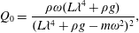 $$\begin{eqnarray}Q_{0}=\frac{\unicode[STIX]{x1D70C}\unicode[STIX]{x1D714}(L\unicode[STIX]{x1D706}^{4}+\unicode[STIX]{x1D70C}g)}{(L\unicode[STIX]{x1D706}^{4}+\unicode[STIX]{x1D70C}g-m\unicode[STIX]{x1D714}^{2})^{2}},\end{eqnarray}$$
and
 $$\begin{eqnarray}C_{g}=\frac{2L\unicode[STIX]{x1D706}^{3}\unicode[STIX]{x1D714}}{L\unicode[STIX]{x1D706}^{4}+\unicode[STIX]{x1D70C}g}+\frac{\unicode[STIX]{x1D714}}{2\unicode[STIX]{x1D706}}\left[1+\frac{2\unicode[STIX]{x1D706}H}{\sinh (2\unicode[STIX]{x1D706}H)}\right]\frac{L\unicode[STIX]{x1D706}^{4}+\unicode[STIX]{x1D70C}g-m\unicode[STIX]{x1D714}^{2}}{L\unicode[STIX]{x1D706}^{4}+\unicode[STIX]{x1D70C}g}\end{eqnarray}$$
is the group velocity for the flexural gravity wave. The radiation coefficients
 $R_{j}^{+}$
and
 $R_{j}^{-}$
in (A 6) can be obtained by letting
 $x\rightarrow \pm \infty$
in (3.46). We have
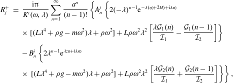 $$\begin{eqnarray}\displaystyle R_{j}^{+} & = & \displaystyle \frac{\text{i}\unicode[STIX]{x03C0}}{K^{\prime }(\unicode[STIX]{x1D714},\unicode[STIX]{x1D706})}\mathop{\sum }_{n=1}^{\infty }\frac{a^{n}}{(n-1)!}\left\{A_{n}^{j}\left\{2(-\unicode[STIX]{x1D706})^{n-1}\text{e}^{-\unicode[STIX]{x1D706}(z_{0}+2H)+\text{i}\unicode[STIX]{x1D706}x_{0}}\right.\right.\nonumber\\ \displaystyle & & \displaystyle \times \left.[(L\unicode[STIX]{x1D706}^{4}+\unicode[STIX]{x1D70C}g-m\unicode[STIX]{x1D714}^{2})\unicode[STIX]{x1D706}+\unicode[STIX]{x1D70C}\unicode[STIX]{x1D714}^{2}]+L\unicode[STIX]{x1D70C}\unicode[STIX]{x1D714}^{2}\unicode[STIX]{x1D706}^{2}\left[\frac{\unicode[STIX]{x1D706}{\mathcal{G}}_{1}(n)}{{\mathcal{I}}_{1}}-\frac{{\mathcal{G}}_{1}(n-1)}{{\mathcal{I}}_{2}}\right]\right\}\nonumber\\ \displaystyle & & \displaystyle -\,B_{n}^{j}\left\{2\unicode[STIX]{x1D706}^{n-1}\text{e}^{\unicode[STIX]{x1D706}z_{0}+\text{i}\unicode[STIX]{x1D706}x_{0}}\right.\nonumber\\ \displaystyle & & \displaystyle \times \left.\left.[(L\unicode[STIX]{x1D706}^{4}+\unicode[STIX]{x1D70C}g-m\unicode[STIX]{x1D714}^{2})\unicode[STIX]{x1D706}+\unicode[STIX]{x1D70C}\unicode[STIX]{x1D714}^{2}]+L\unicode[STIX]{x1D70C}\unicode[STIX]{x1D714}^{2}\unicode[STIX]{x1D706}^{2}\left[\frac{\unicode[STIX]{x1D706}{\mathcal{G}}_{2}(n)}{{\mathcal{I}}_{1}}+\frac{{\mathcal{G}}_{2}(n-1)}{{\mathcal{I}}_{2}}\right]\right\}\right\},\qquad\end{eqnarray}$$
and
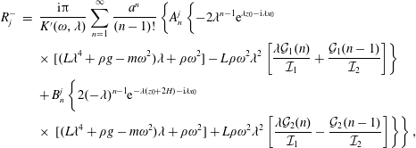 $$\begin{eqnarray}\displaystyle R_{j}^{-} & = & \displaystyle \frac{\text{i}\unicode[STIX]{x03C0}}{K^{\prime }(\unicode[STIX]{x1D714},\unicode[STIX]{x1D706})}\mathop{\sum }_{n=1}^{\infty }\frac{a^{n}}{(n-1)!}\left\{A_{n}^{j}\left\{-2\unicode[STIX]{x1D706}^{n-1}\text{e}^{\unicode[STIX]{x1D706}z_{0}-\text{i}\unicode[STIX]{x1D706}x_{0}}\right.\right.\nonumber\\ \displaystyle & & \displaystyle \times \left.[(L\unicode[STIX]{x1D706}^{4}+\unicode[STIX]{x1D70C}g-m\unicode[STIX]{x1D714}^{2})\unicode[STIX]{x1D706}+\unicode[STIX]{x1D70C}\unicode[STIX]{x1D714}^{2}]-L\unicode[STIX]{x1D70C}\unicode[STIX]{x1D714}^{2}\unicode[STIX]{x1D706}^{2}\left[\frac{\unicode[STIX]{x1D706}{\mathcal{G}}_{1}(n)}{{\mathcal{I}}_{1}}+\frac{{\mathcal{G}}_{1}(n-1)}{{\mathcal{I}}_{2}}\right]\right\}\nonumber\\ \displaystyle & & \displaystyle +\,B_{n}^{j}\left\{2(-\unicode[STIX]{x1D706})^{n-1}\text{e}^{-\unicode[STIX]{x1D706}(z_{0}+2H)-\text{i}\unicode[STIX]{x1D706}x_{0}}\right.\nonumber\\ \displaystyle & & \displaystyle \times \left.\left.[(L\unicode[STIX]{x1D706}^{4}+\unicode[STIX]{x1D70C}g-m\unicode[STIX]{x1D714}^{2})\unicode[STIX]{x1D706}+\unicode[STIX]{x1D70C}\unicode[STIX]{x1D714}^{2}]+L\unicode[STIX]{x1D70C}\unicode[STIX]{x1D714}^{2}\unicode[STIX]{x1D706}^{2}\left[\frac{\unicode[STIX]{x1D706}{\mathcal{G}}_{2}(n)}{{\mathcal{I}}_{1}}-\frac{{\mathcal{G}}_{2}(n-1)}{{\mathcal{I}}_{2}}\right]\right\}\right\},\qquad\end{eqnarray}$$
where the prime in
 $K^{\prime }(\unicode[STIX]{x1D714},\unicode[STIX]{x1D706})$
denotes partial derivative with respect to
 $\unicode[STIX]{x1D706}$
.
Appendix B. The far field formula for the wave exciting force
By noticing the condition in (2.5), the wave exciting force in (3.72) can be given as
 $$\begin{eqnarray}f_{E,j}=-\text{i}\unicode[STIX]{x1D714}\unicode[STIX]{x1D70C}\int _{S_{0}}\left(\unicode[STIX]{x1D719}_{0}\frac{\unicode[STIX]{x2202}\unicode[STIX]{x1D719}_{j}}{\unicode[STIX]{x2202}n}-\unicode[STIX]{x1D719}_{j}\frac{\unicode[STIX]{x2202}\unicode[STIX]{x1D719}_{0}}{\unicode[STIX]{x2202}n}\right)\,\text{d}S.\end{eqnarray}$$
As for the damping coefficient, this can be converted as
 $$\begin{eqnarray}\displaystyle f_{E,j} & = & \displaystyle \text{i}\unicode[STIX]{x1D714}\unicode[STIX]{x1D70C}\int _{S_{+\infty }+S_{-\infty }}\left(\unicode[STIX]{x1D719}_{0}\frac{\unicode[STIX]{x2202}\unicode[STIX]{x1D719}_{j}}{\unicode[STIX]{x2202}n}-\unicode[STIX]{x1D719}_{j}\frac{\unicode[STIX]{x2202}\unicode[STIX]{x1D719}_{0}}{\unicode[STIX]{x2202}n}\right)\,\text{d}S\nonumber\\ \displaystyle & & \displaystyle +\,\text{i}\frac{L}{\unicode[STIX]{x1D714}}\left[\left(\frac{\unicode[STIX]{x2202}^{4}\unicode[STIX]{x1D719}_{0}}{\unicode[STIX]{x2202}x^{3}\unicode[STIX]{x2202}z}\frac{\unicode[STIX]{x2202}\unicode[STIX]{x1D719}_{j}}{\unicode[STIX]{x2202}z}-\frac{\unicode[STIX]{x2202}^{3}\unicode[STIX]{x1D719}_{0}}{\unicode[STIX]{x2202}x^{2}\unicode[STIX]{x2202}z}\frac{\unicode[STIX]{x2202}^{2}\unicode[STIX]{x1D719}_{j}}{\unicode[STIX]{x2202}x\unicode[STIX]{x2202}z}+\frac{\unicode[STIX]{x2202}^{3}\unicode[STIX]{x1D719}_{j}}{\unicode[STIX]{x2202}x^{2}\unicode[STIX]{x2202}z}\frac{\unicode[STIX]{x2202}^{2}\unicode[STIX]{x1D719}_{0}}{\unicode[STIX]{x2202}x\unicode[STIX]{x2202}z}-\frac{\unicode[STIX]{x2202}^{4}\unicode[STIX]{x1D719}_{j}}{\unicode[STIX]{x2202}x^{3}\unicode[STIX]{x2202}z}\frac{\unicode[STIX]{x2202}\unicode[STIX]{x1D719}_{0}}{\unicode[STIX]{x2202}z}\right)_{z=0}\right]_{x=-\infty }^{x=+\infty }.\qquad\end{eqnarray}$$
At
 $x\rightarrow \pm \infty$
,
 $\unicode[STIX]{x1D719}_{0}$
can be written in the following asymptotic form
 $$\begin{eqnarray}\unicode[STIX]{x1D719}_{0}=\left\{\begin{array}{@{}ll@{}}\displaystyle T\text{e}^{-\text{i}\unicode[STIX]{x1D706}x}\unicode[STIX]{x1D713}(z) & \text{at }x\rightarrow +\infty \\ \displaystyle (I\text{e}^{-\text{i}\unicode[STIX]{x1D706}x}+R\text{e}^{+\text{i}\unicode[STIX]{x1D706}x})\unicode[STIX]{x1D713}(z) & \text{at }x\rightarrow -\infty .\end{array}\right.\end{eqnarray}$$
Thus (B 2) becomes
 $$\begin{eqnarray}f_{E,j}=2I\unicode[STIX]{x1D70C}\unicode[STIX]{x1D714}Q_{0}C_{g}R_{j}^{-}.\end{eqnarray}$$
The transmission and reflection coefficients in (B 3) can be obtained by letting
 $x\rightarrow \pm \infty$
in (3.46) and (3.66). We obtain
 $$\begin{eqnarray}\displaystyle & \displaystyle T=T_{0}+I\times T_{c}, & \displaystyle\end{eqnarray}$$
 $$\begin{eqnarray}\displaystyle & \displaystyle R=R_{0}+I\times R_{c}, & \displaystyle\end{eqnarray}$$
where
 $T_{0}$
and
 $R_{0}$
are due to
 $\unicode[STIX]{x1D719}_{D}^{2}$
and can be obtained through equations similar to (A 9) and (A 10);
 $T_{c}$
and
 $R_{c}$
are due to
 $\unicode[STIX]{x1D719}_{D}^{1}$
and can be obtained from (3.66)
 $$\begin{eqnarray}\displaystyle & \displaystyle T_{c}=1+\frac{\text{i}\unicode[STIX]{x03C0}}{K^{\prime }(\unicode[STIX]{x1D714},\unicode[STIX]{x1D706})}L\unicode[STIX]{x1D706}^{5}\tanh (\unicode[STIX]{x1D706}H)\left(\frac{\unicode[STIX]{x1D706}^{2}}{{\mathcal{I}}_{1}}+\frac{1}{{\mathcal{I}}_{2}}\right), & \displaystyle\end{eqnarray}$$
 $$\begin{eqnarray}\displaystyle & \displaystyle R_{c}=-\frac{\text{i}\unicode[STIX]{x03C0}}{K^{\prime }(\unicode[STIX]{x1D714},\unicode[STIX]{x1D706})}L\unicode[STIX]{x1D706}^{5}\tanh (\unicode[STIX]{x1D706}H)\left(\frac{\unicode[STIX]{x1D706}^{2}}{{\mathcal{I}}_{1}}-\frac{1}{{\mathcal{I}}_{2}}\right). & \displaystyle\end{eqnarray}$$
Appendix C. Haskind relation for wave exciting force
Substituting
 $\unicode[STIX]{x1D711}=\unicode[STIX]{x1D719}_{I}+\unicode[STIX]{x1D719}_{D}^{1}$
and
 $\unicode[STIX]{x1D719}_{D}^{2}$
into (3.72), and noticing the condition in (2.5), we can write the wave exciting force as
 $$\begin{eqnarray}f_{E,j}=-\text{i}\unicode[STIX]{x1D714}\unicode[STIX]{x1D70C}\int _{S_{0}}\left(\unicode[STIX]{x1D711}\frac{\unicode[STIX]{x2202}\unicode[STIX]{x1D719}_{j}}{\unicode[STIX]{x2202}n}+\unicode[STIX]{x1D719}_{D}^{2}\frac{\unicode[STIX]{x2202}\unicode[STIX]{x1D719}_{j}}{\unicode[STIX]{x2202}n}\right)\,\text{d}S.\end{eqnarray}$$
Applying Green’s second identity to
 $\unicode[STIX]{x1D719}_{D}^{2}$
and
 $\unicode[STIX]{x1D719}_{j}$
over the fluid boundary
 $S$
, we have
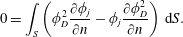 $$\begin{eqnarray}0=\int _{S}\left(\unicode[STIX]{x1D719}_{D}^{2}\frac{\unicode[STIX]{x2202}\unicode[STIX]{x1D719}_{j}}{\unicode[STIX]{x2202}n}-\unicode[STIX]{x1D719}_{j}\frac{\unicode[STIX]{x2202}\unicode[STIX]{x1D719}_{D}^{2}}{\unicode[STIX]{x2202}n}\right)\,\text{d}S.\end{eqnarray}$$
Noticing that both
 $\unicode[STIX]{x1D719}_{D}^{2}$
and
 $\unicode[STIX]{x1D719}_{j}$
represent the outgoing wave at infinity and satisfy the ice sheet and seabed conditions, we can rewrite (C 2) as
 $$\begin{eqnarray}\displaystyle 0 & = & \displaystyle \int _{S_{0}}\left(\unicode[STIX]{x1D719}_{D}^{2}\frac{\unicode[STIX]{x2202}\unicode[STIX]{x1D719}_{j}}{\unicode[STIX]{x2202}n}-\unicode[STIX]{x1D719}_{j}\frac{\unicode[STIX]{x2202}\unicode[STIX]{x1D719}_{D}^{2}}{\unicode[STIX]{x2202}n}\right)\,\text{d}S\nonumber\\ \displaystyle & & \displaystyle +\,\frac{L}{\unicode[STIX]{x1D70C}\unicode[STIX]{x1D714}^{2}}\left[\left(\frac{\unicode[STIX]{x2202}^{4}\unicode[STIX]{x1D719}_{D}^{2}}{\unicode[STIX]{x2202}x^{3}\unicode[STIX]{x2202}z}\frac{\unicode[STIX]{x2202}\unicode[STIX]{x1D719}_{j}}{\unicode[STIX]{x2202}z}-\frac{\unicode[STIX]{x2202}^{3}\unicode[STIX]{x1D719}_{D}^{2}}{\unicode[STIX]{x2202}x^{2}\unicode[STIX]{x2202}z}\frac{\unicode[STIX]{x2202}^{2}\unicode[STIX]{x1D719}_{j}}{\unicode[STIX]{x2202}x\unicode[STIX]{x2202}z}+\frac{\unicode[STIX]{x2202}^{3}\unicode[STIX]{x1D719}_{j}}{\unicode[STIX]{x2202}x^{2}\unicode[STIX]{x2202}z}\frac{\unicode[STIX]{x2202}^{2}\unicode[STIX]{x1D719}_{D}^{2}}{\unicode[STIX]{x2202}x\unicode[STIX]{x2202}z}-\frac{\unicode[STIX]{x2202}^{4}\unicode[STIX]{x1D719}_{j}}{\unicode[STIX]{x2202}x^{3}\unicode[STIX]{x2202}z}\frac{\unicode[STIX]{x2202}\unicode[STIX]{x1D719}_{D}^{2}}{\unicode[STIX]{x2202}z}\right)_{z=0}\right]_{x=0^{+}}^{x=0^{-}}.\nonumber\\ \displaystyle & & \displaystyle\end{eqnarray}$$
Through the condition in (2.4) for
 $\unicode[STIX]{x1D719}_{D}^{2}$
and
 $\unicode[STIX]{x1D719}_{j}$
at the crack, (C 3) gives
 $$\begin{eqnarray}\int _{S_{0}}\left(\unicode[STIX]{x1D719}_{D}^{2}\frac{\unicode[STIX]{x2202}\unicode[STIX]{x1D719}_{j}}{\unicode[STIX]{x2202}n}\right)\,\text{d}S=\int _{S_{0}}\left(\unicode[STIX]{x1D719}_{j}\frac{\unicode[STIX]{x2202}\unicode[STIX]{x1D719}_{D}^{2}}{\unicode[STIX]{x2202}n}\right)\,\text{d}S.\end{eqnarray}$$
Substituting this into (C 1) and noticing the condition in (3.69), we can obtain the Haskind relation for
 $f_{E,j}$
as
 $$\begin{eqnarray}f_{E,j}=-\text{i}\unicode[STIX]{x1D714}\unicode[STIX]{x1D70C}\int _{S_{0}}\left(\unicode[STIX]{x1D711}\frac{\unicode[STIX]{x2202}\unicode[STIX]{x1D719}_{j}}{\unicode[STIX]{x2202}n}-\unicode[STIX]{x1D719}_{j}\frac{\unicode[STIX]{x2202}\unicode[STIX]{x1D711}}{\unicode[STIX]{x2202}n}\right)\,\text{d}S,\end{eqnarray}$$
which is similar to that for an infinitely extended free surface (Mei, Stiassnie & Yue Reference Mei, Stiassnie and Yue2005). It should be noticed that in the free surface problem
 $\unicode[STIX]{x1D711}$
includes the incident potential
 $\unicode[STIX]{x1D719}_{I}$
from infinity only, while in (C 5)
 $\unicode[STIX]{x1D711}$
contains not only
 $\unicode[STIX]{x1D719}_{I}$
but also its diffraction potential
 $\unicode[STIX]{x1D719}_{D}^{1}$
by the crack.