Introduction
Landscape shifts caused by human activities promote forest loss and fragmentation, with such activities promoted primarily by deforestation due to changes in land use. These spatial shifts reduce original vegetation and, in extreme cases, result in the complete disappearance of forest remnants (Tapia-Armijos et al., Reference Tapia-Armijos, Homeier, Espinoza, Leuschner and de la Cruz2015; Hansen et al. Reference Hansen, Wang, Xiao-Peng, Tyukavina, Turubanova, Potapov and Stehman2020). Depending on the intensity and type of deforestation, native vegetation patches may be left immersed in anthropised landscapes (Guevara et al. Reference Guevara, Laborde and Sánchez-Ríos2004). Aiming to disentangle how ecological processes involving deforestation affect biodiversity, increasing landscape-scale efforts have been made (Mesquita et al. Reference Mesquita, Bernardino, Bobrowiec, Salomão and Cornelius2025; Rivera-Duarte et al. Reference Rivera-Duarte, Salomão, Castillo-Pérez, Von Thaden, Monteros and Favila2025; Salomão et al. Reference Salomão, Alvarado, Maia, Oliveira, Linzmeier and Iannuzzi2024; Souza et al., Reference Souza, França, Barlow, Dodonov, Santos, Faria and Baumgarten2020). Landscape composition – such as the amount of native and non-native forest cover – serves as an excellent proxy to assess how the availability of native and non-native vegetation drives ecological patterns. The amount of native vegetation cover plays a determinant role in species diversity throughout the ecosystems (Mesquita et al. Reference Mesquita, Bernardino, Bobrowiec, Salomão and Cornelius2025; Rivera-Duarte et al. Reference Rivera-Duarte, Salomão, Castillo-Pérez, Von Thaden, Monteros and Favila2025; Salomão et al. Reference Salomão, Alvarado, Baena-Díaz, Favila, Iannuzzi, Liberal, Santos, Vaz-de-Mello and González-Tokman2019). Besides the amount of land use, its distribution in space (i.e., landscape configuration) can provide key information regarding the capacity of ecological assemblages to overcome and thrive throughout the different distribution of land uses across mosaics (Burel and Baudry Reference Burel and Baudry2003). For example, in tropical rainforests of South America, beetle assemblages are highly sensitive to changes in the amount of forest edges between native vegetation and anthropogenic land uses (Salomão et al. Reference Salomão, Alvarado, Maia, Oliveira, Linzmeier and Iannuzzi2024; Souza et al. Reference Souza, França, Barlow, Dodonov, Santos, Faria and Baumgarten2020). Considering fragmented landscapes and the Single Large or Several Small (SLOSS) debate, the amount and spatial distribution of original vegetation patches are determinants for ecological assemblages’ diversity patterns (Riva and Fahrig Reference Riva and Fahrig2022), reinforcing the importance to assess forest fragmentation from a landscape perspective. Landscape changes caused by deforestation have also been associated with shifts in the temporal distribution of species, such as monthly variation throughout the year or among long-term intervals (Collins et al. Reference Collins, Banks-Leite, Brudvig, Cook, Damschen, Andrade, Austin, Camargo, Driscoll, Laurance, Nicholls and Orrock2016; Da Silva et al. Reference Da Silva, Salomão, González-Tokman, Neves and Favila2023; Rivera-Duarte et al. Reference Rivera-Duarte, Salomão, Castillo-Pérez, Von Thaden, Monteros and Favila2025). Taken together, these examples highlight that studies examining landscape shifts associated with changes in diversity and assemblages throughout spatial and temporal scales can provide highly relevant information that allows us to understand how certain human activities affect these ecological mechanisms.
Species are known to exhibit heterogeneous spatial distributions, and shifts in the amount and distribution of land uses can exacerbate this pattern by constraining individuals’ dispersal and habitat availability (Barton et al. Reference Barton, Cunningham, Manning, Gibb, Lindenmayer and Didham2013). In this context, spatial beta diversity – defined as the variation in species composition among the sites (Morin Reference Morin2011) – offers a valuable framework for understanding community structure. Beta diversity can be partitioned into two components: species turnover (i.e., replacement of species between sites) and nestedness (i.e., differences due to species loss or gain); both components provide insights into the mechanism driving biodiversity change (Bevilacqua and Terlizzi Reference Bevilacqua and Terlizzi2019). Extending this concept throughout temporal scales, temporal beta diversity integrates temporal dimensions, allowing the evaluation of how assemblages vary not only among sites but also across sampling periods (Da Silva et al. Reference Da Silva, Salomão, González-Tokman, Neves and Favila2023). This temporal and spatial perspective is particularly relevant throughout anthropogenic landscapes, where communities are potentially subject to dynamic processes such as local extinctions, colonisation events, and seasonal fluctuations in resource availability. By jointly considering spatial and temporal turnover, beta diversity provides a more comprehensive understanding of how spatial changes in land cover influence community heterogeneity, stability, and resilience through time (Da Silva et al. Reference Da Silva, Salomão, González-Tokman, Neves and Favila2023; Rivera-Duarte et al. Reference Rivera-Duarte, Salomão, Castillo-Pérez, Von Thaden, Monteros and Favila2025).
Changes in diversity can be analysed using indicator groups, which provide for quantifying species’ responses to human activities in different environments (Favila and Halffter Reference Favila and Halffter1997; Kremen Reference Kremen1992). Among insects, the beetles of the subfamily Scarabaeinae (Coleoptera: Scarabaeidae) have been widely proposed as a model indicator taxon in biodiversity assessments (Favila and Halffter Reference Favila and Halffter1997; Halffter and Favila Reference Halffter and Favila1983; Noriega et al., Reference Noriega, March-Salas, Castillo, García-Q, Hortal and Santos2021). Most of these studies have primarily focused on insect assemblages inhabiting tropical forests and their anthropogenically modified derivatives. Recent research has refined analytical approaches, enabling the evaluation of ecosystem services provided by dung beetles. For instance, Noriega et al. (2021) documented reductions in richness, abundance, and dung removal rates in disturbed forests. Beyond dung beetles, other families and subfamilies among Coleoptera may also serve as indicators. Correa et al. (Reference Correa, Puker, Lara, Rossa and Krosasaki2019), for example, reported comparable richness, abundance, and biomass of flower chafers (Coleoptera: Cetoniinae) in reserves and urban parks, underscoring the conservation value of native vegetation within urban landscapes.
Members of the subfamily Cetoniinae (Scarabaeidae) represent a promising (Puker et al. Reference Puker, Advincula, Korasaki, Ferreira and Orozco2014), yet understudied, group for examining the impacts of anthropogenic activities on tropical insect assemblages. This group comprises approximately 4,300 species globally (Krajcik Reference Krajcik2011; Maes and Ratcliffe Reference Maes and Ratcliffe2020; Smith, Reference Smith2006), with a wide distribution across tropical and subtropical regions (Howden, Reference Howden1968; Reference Howden1988; Morón and Vaz-de- Mello Reference Morón and Vaz-De-Mello2007). Their ecological habits are closely linked to their modified, membranous mouthparts, which facilitate the consumption of soft fruits, nectar, pollen, and sap (Solís Reference Solís2004), while larvae develop in decomposing organic matter such as leaf litter and decaying wood (Morón et al. Reference Morón, Ratcliffe and Deloya1997). Accordingly, Cetoniinae are classified within the sopro-melliphagous trophic guild (Deloya et al. Reference Deloya, Parra-Tabla and Delfín-González2007). These beetles also exhibit notable flight capabilities, characterised by a unique mechanism in which the elytra are only slightly raised during flight (Šípek et al., Reference Šípek, Fabrizi, Eberle and Ahrens2016). This adaptation confers a high degree of aerodynamic efficiency, enabling them to traverse large distances in short periods of time (Šípek et al., 2016). Their strong association with floral resources suggests that the loss of native plants could negatively impact both the richness and abundance of Cetoniinae species (Chase et al. Reference Chase, McGill, McGlinn, May, Blowes, Xiao, Knight, Purschke and Gotelli2018). The abovementioned characteristics make Cetoniinae suitable candidates for evaluating the impacts of landscape transformation on ecological assemblages. In spite of that, studies examining the effects of landscape transformation driven by anthropogenic activities on Cetoniinae remain limited (Correa et al., Reference Correa, Puker, Lara, Rossa and Krosasaki2019). Thus, it is particularly pertinent to investigate how human-induced disturbance affects the Cetoniinae assemblages throughout time across landscapes with different levels of conservation. The present study adopts a landscape-scale approach and a spatial and temporal perspective on beta diversity, consistent with the framework outlined by Magurran et al. (Reference Magurran, Dornelas, Moyes and Henderson2019), which considers changes in species identity and/or abundance across defined spatial or temporal scales.
The Neotropical rainforests exhibit some of the highest rates of original vegetation loss globally, prompting numerous conservation efforts aimed at safeguarding these ecosystems (Myers et al., Reference Myers, Mittermeier, Mittermeier, Da Fonseca and Kent2000). Despite these initiatives, approximately 90% of tropical forests now exist within anthropogenically altered landscapes (Chadzon et al. Reference Chazdon, Peres, Dent, Sheil, Lugo, Lamb, Stork and Miller2009), resulting in mosaics that maintain variegated conservation levels. A notable example is the Los Tuxtlas Biosphere Reserve (LTBR), located in southern Mexico, which was established in 1998 to halt extensive logging and promote forest conservation (Guevara et al. Reference Guevara, Laborde-Dovalí and Sánchez-Ríos2000, Reference Guevara, Laborde and Sánchez-Ríos2004). Nevertheless, the region experienced significant deforestation and land-use change – primarily due to cattle ranching and government incentives – from the 1950s through the 1980s. As a result, LTBR’s current landscape is characterised by a heterogeneous matrix composed of remnants of primary evergreen forest, secondary vegetation, and extensive cattle pastures (Guevara et al. Reference Guevara, Laborde-Dovalí and Sánchez-Ríos2000). This anthropogenically fragmented environment provides an ideal setting for examining the impacts of landscape transformation on biodiversity.
This study aimed to evaluate the effects of landscape changes on the spatial and temporal patterns of the Cetoniinae beetle assemblage in LTBR. More specifically, we assessed the effect of landscape composition (amounts of forest cover and agricultural cover) and landscape configuration (landscape diversity and the amount of edges) on Cetoniinae species richness, abundance, and spatial and temporal beta diversity. Therefore, our goal was to assess how landscape shifts affect assemblage heterogeneity, which was estimated through measures of spatial and temporal beta diversity, and species composition structure, which included species identity, abundance, and distribution. We hypothesised that landscape disturbance would impair ecological stability and affect the Cetoniinae assemblage structure. Based on this hypothesis, we expected that landscapes with lower amounts of forest cover, higher amounts of agriculture cover, edge areas, and higher landscape diversity would show (1) a lower number of Cetoniinae species and individuals due to reduced habitat quality and resource availability. We also expected that this spatial disturbance would lead to (2) a greater compositional dissimilarity among assemblages, as a result of environmental filtering and increased stochasticity.
Methods
Sampling site
The study was conducted in Los Tuxtlas Biosphere Reserve (LTBR, 18°18′14″–18°37′9″N, 94°45′45″–95°22′20″W) (Figure 1). This reserve is in the northernmost portion of tropical rainforest in the Americas, which is located in the state of Veracruz, Mexico (Figure 1), and is a crucial location for biodiversity conservation. The mean annual temperature is 26°C, and the mean annual rainfall is 4,500 mm. The dry season is from March to May, with an average of 12 mm of rainfall per month, while the rainy season goes from June to February, with an average monthly rainfall of 486 mm (Soto Reference Soto, Guevara, Laborde and Sánchez-Ríos2004).
Geographic location of the Los Tuxtlas Biosphere Reserve (LTBR), Veracruz, Mexico. (A) Map of Mexico showing the state of Veracruz; (B) location of the LTBR within Veracruz; (C) location of the studied landscapes within the reserve.

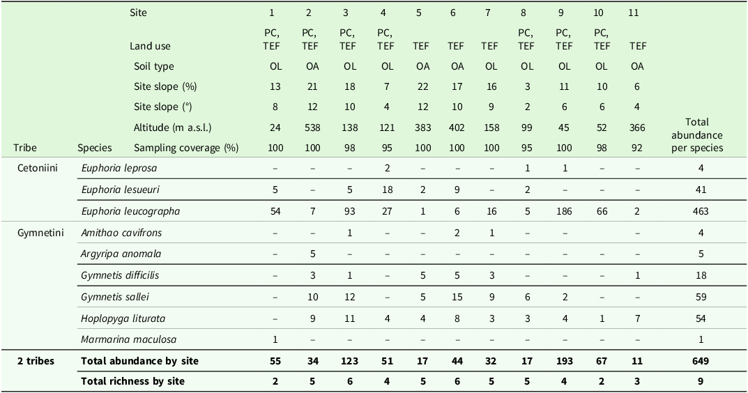
The LTBR region is characterised by soils derived from volcanic material, with Andosols and Luvisols being common on the mountainous slopes, while Gleysols and Fluvisols occur in lowland areas and coastal plains associated with recent alluvial deposits. These soils are generally deep, with high clay and organic matter content, although local variations in drainage and fertility reflect the complex geomorphology of the region (CONABIO 2010; Guevara et al. Reference Guevara, Laborde and Sánchez-Ríos2004; INEGI 2007). For a deeper exploration of LTBR landscapes, soil data of the studied sites were obtained from the edaphological shapefile provided by the ‘Comisión Nacional para el Conocimiento y Uso de la Biodiversidad’ and joined to the sampling site coordinates using QGIS software version 3.42.1, 2023, via the ‘Join Attributes’ function. Also, elevation and slope data were obtained using Google Earth Pro (software version 7.3.6.10201, 2025). For slope, a line was drawn over each trap location, and the elevation profile was extracted. Using the horizontal distance and elevation difference, slope was calculated in Excel both as a percentage [(elevation difference/horizontal distance) × 100] and in degrees [arctan (elevation difference/horizontal difference)]. These data were presented in results sections (Table 1).
Distribution and abundance of Cetoniinae species across forest fragments in the Los Tuxtlas Biosphere Reserve, Veracruz, Mexico. Fragment characteristics include habitat type, soil type, and elevation. PC = cultivated pasture; TEF = tall evergreen forest; OL = Orthic Luvisol; OA = Orthic Andosol; m a.s.l. = metres above sea level

Regarding biodiversity, the LTBR has a high diversity of species, with about 3,000 plant species, 565 birds, 139 mammals, 166 amphibians and reptiles, and 1,117 insects (García Reference García1981; Semarnat 2016). The expansion of agriculture in the region resulted in the loss of about 40% of the native forest vegetation (Guevara et al. Reference Guevara, Laborde-Dovalí and Sánchez-Ríos2000). This overexploitation of natural resources led to the current landscape in the LTBR, which is composed of a mosaic of forest fragments, secondary vegetation, and large areas designated for livestock, agriculture, and urban settlements (Dirzo and García Reference Dirzo and García1992; Mendoza et al. Reference Mendoza and Fay2005; Von Thaden et al. Reference Von Thaden, Laborde, Guevara and Mokodonko-Delgadillo2020). Landscape configuration can promote biodiversity in LTBR, with trees and live fences in the region allowing fauna to move between forest remnants (Mendoza et al. Reference Mendoza and Fay2005 ).
Collection and identification of Cetoniinae beetles
Fieldwork was carried out in the LTBR from May to October 2022, covering the region’s dry and rainy seasons. Cetoniinae beetles were collected with fruit traps (Deloya and Morón Reference Deloya and Morón1994) in 11 landscapes (Figure 1, Table 1). Study landscapes represented a gradient of conservation, which ranged from landscapes with small amounts of native vegetation to landscapes with large amounts of native vegetation (Supplementary material). Fruit traps consisted of plastic containers (1,000 ml in volume) with lids and two 4 × 4 cm openings on the sides to allow the entry of Cetoniinae specimens. Inside each trap, 200 ml of a fermented mixture of pineapple, guava, mango, plantain, yeast and beer was placed, following the protocol described by Morón (Reference Morón1995), to attract beetles. Five traps were deployed within forest patches located in each landscape; each trap was spaced 100 m apart, forming a 500-m transect in each landscape. Traps were suspended from tree branches at a height of approximately 9 metres; specimens were collected monthly, and traps were re-baited during each visit. Following collection, all individuals were preserved in 70% ethanol for subsequent taxonomic analysis. Once beetles were captured by the fruit traps, they remained inside them; depending on the environmental moisture during the collection, individuals were preserved in neither a dry nor a moist state. Although some decomposition could occur, most specimens could still be identified to the species level. This sampling effort resulted in a total of 330 samples (11 landscapes × 5 traps × 6 months).
The beetles were identified at the species level using various taxonomic keys: Euphoria (Orozco Reference Orozco2012); Amithao (Ratcliffe, Reference Ratcliffe2013; Gasca-Álvarez, 2023); Hoplopyga (Shaughney and Ratcliffe, Reference Shaughney and Ratcliffe2015); Gymentis (Ratcliffe, Reference Ratcliffe2018). Fernando Escobar, INECOL, carried out confirmation of species identification. The specimens were deposited in the IEXA ‘Miguel Ángel Morón’ collection of the Instituto de Ecología A. C, Xalapa, Veracruz, Mexico.
Landscape metrics
A PlanetScope satellite image from June 2022 with a spatial resolution of 3 m was classified using the maximum likelihood algorithm to differentiate five land-cover classes across the 11 studied landscapes: forest, agriculture, urban, water, and bare soil. Based on this classification, four landscape descriptors were derived using FRAGSTATS software version 4.2.681: forest cover, agriculture cover, total amount of edge, and the Shannon Diversity Index (SHDI). Forest cover was selected as an indicator of habitat availability and microclimatic stability, particularly relevant for beetle assemblages due to its association with leaf litter, moisture retention, and organic matter inputs (Rivera et al. Reference Rivera, Arellano and Halffter2021). Agriculture cover was included to represent land-use intensification and disturbance, which may affect resource availability and compromise ecological connectivity (Peixoto et al. Reference Peixoto, Barbosa, Martins, Franco, Mata and Korasaki2025). The total amount of edge metric quantifies the perimeter length of landscape patches, serving as a proxy for fragmentation intensity and edge effects, both of which can influence insect movement and habitat functionality (Souza et al. Reference Souza, França, Barlow, Dodonov, Santos, Faria and Baumgarten2020). Finally, SHDI was incorporated as a measure of compositional landscape heterogeneity, which has been positively linked to higher insect diversity and ecological resilience (Salomão et al. Reference Salomão, Alvarado, Maia, Oliveira, Linzmeier and Iannuzzi2024). These metrics provided a spatially explicit characterisation of each site, allowing the assessment of how landscape structure influences beetle assemblage responses. These landscape metrics were obtained at four distinct spatial scales: 150, 250, 350, and 450 m radii, which were used to estimate a clear relationship between landscape metrics and Cetoniinae assemblage variables.
Data analysis
To estimate the sampling effort of the Cetoniinae beetles collected in each of the 11 studied landscapes, sampling coverage estimators were used following Chao et al. (Reference Chao, Gotelli, Hsieh, Sander, Ma, Colwell and Ellison2014). This estimator considered species richness, abundance, and the number of rare species. The estimations were conducted using iNEXT in R software version 4.3.0 (Hsieh et al., Reference Hsieh, Ma and Chao2016; The R Core Team, 2023).
To evaluate the temporal effects of landscape structure and composition on Cetoniinae assemblage heterogeneity, temporal beta diversity was estimated across the 11 studied landscapes. Temporal variation was assessed within each landscape through the Cetoniinae species distribution among the six sampling months. Similarity matrices and dendrograms were constructed for each landscape, and the beta.multi function from the BAT package in R (Cardoso et al., Reference Cardoso, Mammola, Rigal and Carvalho2020) was used to calculate the total beta diversity, as well as the components that explain it (turnover and nestedness). The nestedness component reflected the variation in species richness among sampling months, while the turnover component was related to the temporal species replacement (following Legendre, Reference Legendre2019).
To assess the effect of landscape composition (forest cover and agriculture cover) and landscape configuration (landscape diversity and total amount of edge) on Cetoniinae species richness, abundance, and temporal beta diversity (total beta diversity, turnover, and nestedness components), statistical models were performed. Data obtained from each of the 11 landscapes represented a replicate; landscape configuration and composition metrics were the predictor variables, while Cetoniinae assemblage data were the predicted ones. To determine the most appropriate spatial scale (150, 250, 350, or 450 m radius) for evaluating the effect of landscape variables on the response variables, a multiscale approach was used (Mesquita et al. Reference Mesquita, Bernardino, Bobrowiec, Salomão and Cornelius2025; Salomão et al. Reference Salomão, Alvarado, Baena-Díaz, Favila, Iannuzzi, Liberal, Santos, Vaz-de-Mello and González-Tokman2019). Such an approach has been used in other landscape-scale studies involving insect groups in tropical ecosystems and consists of selecting the spatial scale for each landscape variable that presents the strongest relationship with each response variable (i.e., highest r2). To avoid collinearity among independent variables, we calculated the variance inflation factor (VIF) of the models. Only variables with VIF values < 5 were retained, as this threshold indicates the absence of collinearity (Gareth et al. Reference Gareth, Hastie, Tibshirani and Witten2013). In addition, the statistical models were reduced with the Akaike information criteria (AIC) to obtain the minimal adequate models. Predictor variables were ranked according to their p-value, and those with p < 0.05 were kept in the best and most parsimonious model (Zuur et al. Reference Zuur, Ieno, Walker, Saveliev and Smith2009). After filtering the pool of predictor variables, statistical assumptions were tested to select the model that best fit the data distribution. Data normality was checked with the Shapiro-Wilk test; homoscedasticity was checked with ncvTest in the car package (Fox and Weisberg Reference Fox and Weisberg2019); dispersion of the residuals was checked (Residual deviance/Residual d. f. > 2); outliers were visualised by using the Cooks’ Distance (outliers: Cooks’ Distance > 1.0). Statistical models were performed in R software (R Core Team 2023); detailed information about the chosen models is provided in Table S1.
In order to assess how landscapes clustered Cetoniinae assemblage data, a Similarity Profile (SIMPROF) was conducted. This approach is a proxy of spatial beta diversity and was used to analyse the similarity between Cetoniinae assemblage structures (i.e., species distribution and their abundances) among the studied landscapes, using total data from each landscape as a sample. SIMPROF compares similarities between each pair of samples and classifies them from lowest to highest (Clarke et al., Reference Clarke, Somerfield and Gorley2008). Statistically significant groups were structured based on a less than 5% probability of being grouped randomly, according to the provided data. Species abundance data from each landscape were used to perform SIMPROF in both approaches (sites and species). The Bray-Curtis similarity index, sensitive to species abundance, was used for SIMPROF. This analysis was performed using Primer software version 6.0 (Clarke and Gorley Reference Clarke and Gorley2006). For an explorative purpose, landscape variables at the scales that best explained variation of Cetoniinae beta diversity were provided in the SIMPROF figure, which is included in the results section.
Results
A total of 649 individuals representing six genera and nine species belonging to two tribes (Cetoniini and Gymnetini) were collected (Table 1). The tribe Cetoniini exhibited the highest species richness and abundance, with three species and 508 individuals recorded. Euphoria Leucographa (Gory and Percheron, 1833) was the most abundant species, accounting for 463 individuals, followed by Gymnetis sallei Schaum, 1849, with 59 individuals, and Hoplopyga liturata (Olivier, 1789) with 54 individuals (Table 1). In contrast, Amithao cavifrons (Burmeister, 1842), Euphoria leprosa Burmeister, 1842, and Marmarina maculosa (Olivier, 1789) were the least abundant species, represented by four, two and one individuals, respectively (Table 1). Sampling coverage was high across all studied landscapes, ranging between 92% and 100% per landscape (Table 1).
Overall, species richness exhibited marked temporal fluctuations across months and landscapes (Supplementary material). Species richness ranged between two and six species per landscape. Most landscapes showed high species richness during the middle of the sampling period, between July and September, followed by a consistent decline in October.
Landscape effects on assemblage diversity and abundance
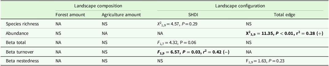
Interestingly, landscape composition (amount of forest and agriculture cover) did not affect any metric of Cetoniinae assemblage (Table 2). Moreover, Cetoniinae species richness, total beta diversity and nestedness component were not affected by any landscape variables (Table 2). The total edge of landscapes affected Cetoniinae abundance; landscapes with larger amounts of edge comprised more abundant Cetoniinae assemblages (Figure 2A, Table 2). Landscape diversity negatively affected species turnover throughout months – spatially less diverse landscapes had lower Cetoniinae temporal species turnover compared to spatially more diverse landscapes (Figure 2B, Table 2).
Statistical models evaluating the effects of landscape composition (forest amount and agricultural area) and configuration (SHDI and total edge) on Cetoniinae species richness, abundance, total beta diversity, and its components (turnover and nestedness) in landscapes of the Los Tuxtlas Biosphere Reserve, Veracruz, Mexico. Significant effects are shown in bold; ‘+’ indicates a positive relationship and ‘–’ a negative relationship. NA = variables excluded due to multicollinearity; NS = variables excluded based on the Akaike information criterion (AIC)

Significant relationships between landscape diversity (Shannon Diversity Index, SHDI) and temporal species turnover (β-turnover) (A) and between total edge and Cetoniinae abundance (B).

The SIMPROF analysis divided the Cetoniinae assemblages recorded into two statistically distinct groups (Figure 3). Landscapes with lower amounts of forest cover and higher amounts of edge (Figure 3, group A) grouped with 41% similarity, while the remaining landscapes, which presented high amounts of forest cover and low amounts of edge, clustered together with 37% similarity (Figure 3, group B). In Group A, E. Leucographa was the most abundant species, while in Group B, G. difficilis, G. Sallei, H. liturata, and M. maculosa was the most abundant species (Figure 3).
Dendrogram illustrating the clustering of the 11 landscapes based on Cetoniinae assemblage structure (species composition and abundance). Dashed lines indicate statistically significant clusters (P < 0.05).

Discussion
Landscape shifts that come from the forest loss and fragmentation are one of the most alarming consequences of anthropogenic activity on biodiversity, affecting species distribution patterns in the native vegetation remnants (Cardoso et al. Reference Cardoso, Almeida, Matos, Edwards and Santos2025; Riva and Fahrig Reference Riva and Fahrig2022; Tabarelli et al. Reference Tabarelli, Peres and Melo2012). Besides the well-known decreases in diversity, abundances, and shifts in species composition of ecological assemblages because of spatial changes in landscape (Almeida-Gomes et al. Reference Almeida-Gomes, Vieira, Duarte Rocha, Metzger and De Coster2016; Huikkonen et al. Reference Huikkonen, Helle and Elo2019; Jain et al. Reference Jain, Lim and Webb2017; Kaushik et al. Reference Kaushik, Tiwari and Manisha2022), these spatial processes also affect temporal assemblage heterogeneity. This study provides two important findings: (a) spatially diverse landscapes promote a decrease of species turnover throughout time; and (b) landscapes with higher amounts of edge maintain more abundant Cetoniinae assemblages compared to landscapes with lower amounts of edges. These findings indicate landscape configuration, but not composition, is an important driver of Cetoniinae diversity patterns in the hyperfragmented landscape of LTBR. Our results reinforce a scenario in which the effects of spatial shifts on biodiversity are dependent on how land uses are distributed and in which such distribution affects temporal dynamics of ecological assemblages.
When considering shifts in landscape configuration, there is temporal heterogeneity of ecological assemblages in more stable environments, maintaining more homogenous assemblages (Da Silva et al. Reference Da Silva, Salomão, González-Tokman, Neves and Favila2023; Morón and Marquéz Reference Morón and Marquéz2012; Morón et al. Reference Morón, Ratcliffe and Deloya1997). We found that changes in the landscape diversity affected Cetoniinae heterogeneity, and spatially more diverse landscapes comprised assemblages with lower temporal species turnover than less diverse landscapes did. Our results may be analysed under the light of Cetoniinae beetles’ biological cycle, which are composed of species with different activity peaks throughout the year (Orozco Reference Orozco2012; Ratcliffe Reference Ratcliffe2017; Shaughney and Ratcliffe Reference Shaughney and Ratcliffe2015). Furthermore, anthropogenic disturbance in tropical rainforests modulates seasonal activity patterns of insects (Morón Reference Morón1995; Morón and Gómez-Rojas Reference Morón and Gómez-Rojas2011). Under this rationale, spatially diverse landscapes in LTBR comprise a mosaic of different land uses, such as pasturelands, primary forests, secondary forests, citrus, and pepper plantations. Considering the strict environmental needs of Cetoniinae beetles (Deloya et al. Reference Deloya, Parra-Tabla and Delfín-González2007; Solís Reference Solís2004), landscapes with larger amounts of homogeneous land use (i.e., lower landscape diversity) could represent a more stable condition to sustain complex assemblages with different seasonal peaks – therefore presenting a high species turnover. Smaller forest fragments tend to have lower species diversity than larger ones (Filgueiras et al. Reference Filgueiras, Iannuzzi and Leal2011; Hill et al. Reference Hill, Gray, Vun Khen, Benedict, Tawatao and Hamer2011; Zhu et al. Reference Zhu, Xu, Wang and Li2004), strengthening this hypothesis. Such a perspective supports the idea that heterogeneous landscapes could support a smaller pool of species throughout the year compared to large amounts of specific land uses. For assemblages in which species comprise naturally temporal multimodal peaks of activity – such as the Cetoniinae – it is important to disentangle whether a high heterogeneity of spatiotemporal beta diversity is related to more conserved or more disturbed landscapes.
Contrary to our predictions, landscapes with higher amounts of edges maintained more abundant Cetoniinae assemblages compared to those with lower amounts of edges. While this scenario is intriguing, it converges with other patterns observed in tropical ecosystems. For example, in South American drylands, a higher diversity of herbivorous beetles was recorded in landscapes with high amounts of edges (Salomão et al. Reference Salomão, Alvarado, Maia, Oliveira, Linzmeier and Iannuzzi2024); also, Coleoptera, Diptera, and Hymenoptera were more abundant in edge areas than in the interior of native vegetation within the Chaco ecosystem (González et al. Reference González, Salvo and Valladares2017). Forest edges are often composed of ruderal plant species, which can promote high abundances of opportunistic and habitat generalist herbivores. As observed in SIMPROF results, E. Leucographa was the most abundant species found in this study, being highly abundant in landscapes with higher amounts of edge. This species is geographically widespread and uses diverse food sources (Cherry and Klein Reference Cherry and Klein1992; Landot Reference Landot1990; Orozco Reference Orozco2012) and tends to be more tolerant to environmental conditions, thriving in contrasting ecosystems (Aguirre-Jaimes et al. Reference Aguirre-Jaimes, López-Acosta and Dirzo2021). Our results suggest that fragmented landscapes with high amounts of edges may benefit the overall abundance of Cetoniinae beetles. Nevertheless, considering the role of superabundant species in ecological patterns (Hillebrand et al. Reference Hillebrand, Bennet and Cadotte2008; Legendre Reference Legendre2019; Souza et al. Reference Souza, França, Barlow, Dodonov, Santos, Faria and Baumgarten2020), our results should be considered with care. The dominance of E. Leucographa in forest edges indicates that a few species are resilient and thrive under the highly fragmented landscapes of LTBR.
Landscapes clustered two markedly distinct Cetoniinae assemblages. One of them comprised Cetoniinae species that were more abundant in landscapes with high amounts of forest cover and low amounts of edge (e.g., G. sallei, H. liturata, G. difficilis, and A. anomala), and the other cluster was dominated by the abovementioned edge-tolerant species, E. Leucographa. A study with dung beetle assemblages of the LTBR suggested that ecological assemblages could face a threshold of recovery when facing landscape conservation scenarios (Rivera et al., Reference Rivera, da Silva and Favila2021). In our study, the cluster that presented abundant species in landscapes with large amounts of forest cover was found in low numbers in the cluster dominated by E. Leucographa. Such a shift in species distribution throughout LTBR landscapes could indicate that the current highly fragmented landscape of the region (Dirzo et al. Reference Dirzo, Young, Galetti, Ceballos, Isaac and Collen2014; Guevara et al. Reference Guevara, Laborde-Dovalí and Sánchez-Ríos2000, Reference Guevara, Laborde and Sánchez-Ríos2004) conserves different species throughout the contrasting landscapes, which could be a product of species environmental requirements. In this sense, for the conservation of the gamma diversity of Cetoniinae in this region, it is important to maintain landscapes with contrasting composition and configuration.
This work represents one of the first efforts to assess the effects of landscape structure on spatial and temporal heterogeneity of Cetoniinae assemblages, offering a significant contribution to our understanding of how forest loss and fragmentation impact insect diversity. Previous studies (Orozco Reference Orozco2012; Solís Reference Solís2004) have emphasised that plants are the primary food source for Cetoniinae, suggesting that habitats with high plant diversity could sustain greater beetle diversity. Although this relationship has been only superficially explored, there is evidence (Puker et al. Reference Puker, Advincula, Korasaki, Ferreira and Orozco2014; Touroult and Le Gall Reference Touroult and Le Gall2013) indicating that vegetation structure may influence habitat preferences, species richness, and abundance within this subfamily. Due to the absence of plant diversity data and limited taxonomic support, we were unable to evaluate this factor in our study sites. Nevertheless, our spatiotemporal perspective provides cues to the role of the amount and distribution of habitats on the distribution of Cetoniinae beetles. We suggest that future studies should incorporate both landscape, environmental, and botanical variables to better understand the mechanisms through which anthropogenic influences the diversity and dynamics of Cetoniinae assemblages.
Supplementary material
The supplementary material for this article can be found at https://doi.org/10.1017/S0266467426100492.
Acknowledgements
We thank UNAM’s Tropical Biology Station ‘Los Tuxtlas’ and its director, Rosamond Coates, for logistical support during fieldwork. We also thank biologist Fernando Escobar, Dr Alfonso Diaz, and Dario Velasco for their help in the fieldwork and Dr Roger Guevara for his help in analysing data. A. Eliorett thanks CONACyT for awarding a doctoral scholarship (609152).
Financial support
This research received no specific grant from any funding agency, commercial or not-for-profit sectors.
Competing interests
The authors declare none.