


I. Introduction
Intuitively, the disagreement of views among analysts is a systematic factor affecting stock returns. However, the sign of the impact of disagreement in analysts’ beliefs on the cross section of stock returns is one of the most controversial issues in finance. Alternative theoretical and empirical frameworks have led to different signs on how disagreement affects stock returns.Footnote 1 In this article, we argue that the conflicting results in the literature have arisen since the price of disagreement risk changes sign over time: we provide robust evidence that it is significantly positive in periods of high disagreement, significantly negative in periods of low disagreement, and insignificant otherwise. In addition, we provide a general equilibrium model that sheds light on why the sign of the price of disagreement risk changes over time, structurally estimate this model, and provide evidence that a key mechanism arising in our model (a flight-to-safety) is present in the data as well.
Our proposed risk factor, aggregate disagreement, is shown in Figure 1.
Figure 1 plots the monthly aggregate disagreement measured as the value-weighted average of stock-level disagreement. Stock-level disagreement is the standard deviation of analysts’ forecasts of the long-term growth rate of earnings per share (EPS). High (low) disagreement months are defined as the months when aggregate disagreement is higher (lower) than the average aggregate disagreement plus (minus) 1 standard deviation; medium-disagreement months are those when aggregate disagreement is in the intermediate range. The 1-standard-deviation bands are shown by the horizontal lines.

FIGURE 1 Long description
The x axis displays time from 1985 m 1 to 2018 m 5 in monthly increments. The y axis ranges from 2.5 to 5.5. The main data series is a blue line labeled Aggregate Dispersion, which fluctuates over time. Three horizontal black lines mark the mean and plus or minus one standard deviation bands. Four vertical gray shaded regions indicate recession periods, occurring around 1985, 1991, 2001, and 2008 to 2009. The aggregate dispersion is highest during the early 1980s and late 2000s, peaking above 5, and lowest in the mid 1990s and early 2000s, dropping near 2.5. The line shows sharp increases during and after recessions, with more volatility after 2008. The legend at the bottom identifies the blue line as Aggregate Dispersion and the gray bands as Recession.
In short, it is the value-weighted average of stock-level disagreement. Stock-level disagreement is the standard deviation of analysts’ forecasts of the long-term growth rate of earnings per share (EPS). This “bottom-up” measure has been used in several recent papers (e.g., Yu (Reference Yu2011), Hong and Sraer (Reference Hong and Sraer2016)) and incorporates the views of a vastly greater number of analysts than “top-down” measures, which are comprised of forecasts of the aggregate earnings growth rate. High (low) disagreement months are defined as months when aggregate disagreement is higher (lower) than the average aggregate disagreement plus (minus) 1 standard deviation; medium-disagreement months are those in the intermediate range.Footnote 2
To study the effects of aggregate disagreement on the cross section of stock returns, we start by estimating the market and aggregate disagreement risk loadings,
$ \beta $
 and
$ \delta $
 using 3-year rolling regressions at the monthly frequency of individual stock returns on excess market returns and 1-month lagged aggregate disagreement. These estimated risk loadings allow us to analyze the price of disagreement risk using three different methods described next.
First, we form 10 portfolios using
$ \delta $
 , the estimated aggregate disagreement loadings. Figure 2 highlights the role played by aggregate disagreement in assets’ returns using the full sample and subsamples comprising low-, medium-, and high-disagreement months.
Figure 2 plots the average monthly value-weighted portfolio returns formed by sorting stocks on their pre-ranking
$ \delta $
 s each month. Pre-ranking
$ \beta $
 and
$ \delta $
 are obtained each month using lagged 3-year rolling data on individual stock returns using the regression:
$ {R}_{i,t}={\alpha}_{i,t}+{\beta}_{i,t}\times {R}_{m,t}+{\delta}_{i,t}\times {\mathrm{Aggregate}\ \mathrm{Disagreement}}_{t-1}+{\unicode{x025B}}_{i,t}. $
 High (low) disagreement months are defined as the months when aggregate disagreement is higher (lower) than the average aggregate disagreement plus (minus) 1 standard deviation; medium-disagreement months are those when aggregate disagreement is in the intermediate range.

FIGURE 2 Long description
Panel A (top-left) labeled All Months shows a slight upward trend in portfolio value weighted excess return as decile delta increases from 1 to 10, with values ranging from about 0.5 to 2. Panel B (top-right) labeled Low Dispersion Months shows a downward trend, with the highest excess return near 3.5 at decile 1, decreasing to near zero at decile 10. Panel C (bottom-left) labeled Medium Dispersion Months shows a flat trend, with excess returns around 1.5 to 2 across all deciles. Panel D (bottom-right) labeled High Dispersion Months shows a strong positive trend, with excess return starting near negative 1.5 at decile 1 and rising to about 4 at decile 10. All panels have x-axes labeled Decile delta from 1 to 10 and y-axes labeled Portfolio value weighted excess return from negative 2 to 4.
For the full sample, there is no significant relation between disagreement and portfolio returns. Limiting our sample to low (high) disagreement months, we observe a clear negative (positive) relationship between disagreement in investors’ beliefs and returns. During low (high) disagreement months, a portfolio of stocks in the highest decile of disagreement loading underperforms (outperforms) a portfolio of stocks in the lowest decile of disagreement loading. In months of medium disagreement, the relationship is unclear.
Second, we examine whether firms’ exposure to aggregate disagreement is related to their characteristics, such as size or value, which are well-established priced factors in the asset pricing literature. For example, one might conjecture that smaller firms have greater exposure to aggregate disagreement, so that, based on size, we might expect higher-disagreement firms to have higher returns. We address this concern by double-sorting on size and exposure to aggregate disagreement; if the compensation for bearing a greater exposure to disagreement holds across size quintiles, then we would have established that the disagreement effect is distinct from the size effect. We perform this double sorting exercise for firms’ disagreement exposure with market beta, size, two alternative measures of value, momentum, a comprehensive measure of market sentiment, and the forecast mean, which is used in the recent literature on “subjective beliefs” to measure analysts’ overreaction to recent fundamental news, and confirm that the price of disagreement risk changes sign in different subsamples of the data as described in the previous paragraph.
Third, to extend the robustness of our findings to a very diverse set of firm characteristics in a multivariate setting, we estimate the price of disagreement risk using all portfolios on Ken French’s web page with at least 10 assets. The portfolios are based on standard factors such as size and value, as well as other characteristics, including investment, repurchases, and others. We find, quite remarkably, that the estimates of the price of risk for 35 of the 36 portfolio sets are very similar to those from the set of 100 beta-delta portfolios that we construct. In particular, the price of risk is positive during high-disagreement months and negative during low-disagreement months; furthermore, it is very stable across the subsamples.
To better understand the changing sign of the price of disagreement risk, we construct a production economy N-asset general equilibrium model in the spirit of Merton’s ICAPM, in which two analysts of different types have heterogeneous beliefs and provide different forecasts of a macroeconomic factor (aggregate earnings growth). Our model has a 1-factor structure: all assets’ cash flows linearly load on a single macroeconomic factor (aggregate earnings), but each asset also has significant idiosyncratic risk. We do not make a distinction between consumers and analysts; that is, we assume that each analyst has the same beliefs as some group of consumers in the economy. Consumers invest their wealth in different assets in the economy and speculate with one another on the relative accuracy of their models’ predictions. The beliefs of each analyst and their relative weight in the economy become state variables in the ICAPM framework whose shifts consumers hedge against. We derive an equilibrium cross-sectional pricing equation for our model, which has three endogenously determined factors. The consumers’ beliefs and weighting process do not appear explicitly, but they affect the factors through the portfolio weights of the consumers’ alternative assets.
The first factor compensates the investor for bearing market risk, similar to the CAPM. The only difference from the standard CAPM is that exposure to market risk is measured by the asset’s cash flow beta relative to the market’s cash flow beta, rather than the stock return beta. The second factor measures the risk premium for bearing the aggregate macroeconomic risk, as well as any undiversified idiosyncratic risk. The third factor is the premium for hedging the risk of shifts in the opportunity set in the ICAPM framework of Merton (Reference Merton1973). In our setup, this term depends on the product of the consumer’s risk aversion and the weighted average of the squared cash-flow beta of each asset and the square of the weight the consumer invests in each asset. We call this term the “squared-beta” factor. The negative sign implies that in periods when the term is large, the risk premium for each asset is smaller. The negative sign arises because the consumer’s wealth grows faster when she invests in higher-cash-flow beta assets; that is, her opportunity set is more attractive from a growth perspective. Consumers’ portfolios display a “flight-to-safety”: during periods of higher disagreement, they choose lower-cash-flow-beta assets. The model implies that risk premiums on assets from the hedging term will be higher when the consumer invests heavily in safer assets.
We structurally estimate our model using data on aggregate earnings growth and the series of aggregate analysts’ disagreements. We find two sets of parameters (one for each type of analyst) that maximize the sum of the likelihoods of each agent type observing the fundamentals, as well as matching the model’s time series of aggregate disagreement to that in the data. We show that analysts’ differences in beliefs about regular high- and low-growth-rate states, as well as a disaster state, capture well the time variation in aggregate earnings disagreement.Footnote 3
Our model has striking implications for the pricing of risk across the cross section of stock returns. The model provides a positive correlation between disagreement in analysts’ forecasts and the price of disagreement risk. The model’s price of disagreement risk has a correlation of 0.45 with the price of disagreement risk from two-stage regressions in the data, even though the price of disagreement risk is not a targeted moment in our estimation. As discussed previously, a crucial part of the model’s mechanism is that wealth allocated to lower-cash-flow-beta assets increases in periods of higher disagreement, thereby lowering the squared-beta hedging term and increasing the risk premium on those assets. We provide support for such a flight-to-safety phenomenon in the data, which is again not a targeted moment of our estimation procedure.
The final exercise that we conduct in the article is an out-of-sample one. Our structural model is estimated using data until September 2016.Footnote 4 We then verify that the prices of risk exhibit similar signs as developed in the in-sample period, based, in particular, on keeping the same intervals of high and low disagreement. From October 2016 to the end of 2021, the aggregate disagreement was in the high range for 43 of 63 months and in the medium range for the remaining months. As predicted by the in-sample results, the price of disagreement risk is positive and statistically significant in the high-disagreement months and insignificant otherwise. We also update our model-based disagreement based on realized earnings in the out-of-sample period, and it shows that analyst disagreement would be mostly high in this period, especially after the catastrophic drop in earnings during the pandemic. It is worth noting that the Fama–French three factors, as well as momentum, have statistically insignificant prices of risk in this period, which makes the disagreement factor even more compelling.
An extensive literature in asset pricing has examined the risk–return trade-off. The capital asset pricing model (CAPM) of Sharpe (Reference Sharpe1964), Lintner (Reference Lintner1965), and Black (Reference Black1972) states that the security’s excess return is proportional to the sensitivity of its return to the market return, denoted by CAPM beta. Jensen, Black, and Scholes (Reference Jensen, Black, Scholes and Jensen1972) point out that “high beta” assets earn lower returns on average. More recently, Frazzini and Pedersen (Reference Frazzini and Pedersen2014) document that a portfolio that holds low-beta assets and shorts high-beta assets earns a positive average return. Hong and Sraer (Reference Hong and Sraer2016) relax the CAPM homogeneous expectation assumption and show that when aggregate disagreement is low, expected return increases with beta as in the CAPM. However, when it is large, the expected return can decrease with beta due to short-sale constraints. It is helpful to note that in Hong and Sraer (Reference Hong and Sraer2016), investors’ opportunity set is constant over time, and the only priced risk factor is the market index. In our setup, aggregate disagreement (AD) varies over time and endogenously affects aggregate investment opportunities. As a result, our article is in the ICAPM framework of Merton (Reference Merton1973), rather than the CAPM framework, and hence AD is a systematically priced factor, which is the primary focus of our article.
On the theoretical front, our article contributes to the growing literature on general equilibrium models with heterogeneous beliefs. Building on the seminal papers of Detemple and Murthy (Reference Detemple and Murthy1994) and Basak (Reference Basak2000), David (Reference David2008) studies the implications of heterogeneous beliefs for the risk premium on the market index within this framework, while Dumas, Kurshev, and Uppal (Reference Dumas, Kurshev and Uppal2009) study the implications for “excess volatility” of the market index. Gallmeyer and Hollifield (Reference Gallmeyer and Hollifield2008) study the implications for asset prices in such a model with an added short-sales constraint, while Burashi, Trojani, and Vedolin (Reference Burashi, Trojani and Vedolin2014) extend the framework to multiple stocks in an exchange economy setting with multiple trees. Baker, Hollifield, and Osambela (Reference Baker, Hollifield and Osambela2016) study investment in a single production technology where the representative agent has Epstein-Zin preferences. This article obtains a tractable equilibrium characterization by working within the Cox, Ingersoll, and Ross (Reference Cox, Ingersoll and Ross1985) framework with multiple firms, each with access to a linear production technology. In particular, the scale of each firm is endogenous, and we explicitly study the riskiness of the market portfolio with changing disagreement of beliefs.Footnote 5
In a new and related set of papers, Malmendier and Nagel (Reference Malmendier and Nagel2016) and Das, Kuhnen, and Nagel (Reference Das, Kuhnen and Nagel2020) examine the origins of the different underlying consumer models in the economy. They provide empirical evidence that different life experiences and various characteristics, such as education, affect beliefs. We would conjecture that analysts’ forecasting models are affected by similar characteristics.
The remainder of this article is organized as follows: In Section II, we describe the data used and provide results of predictability regressions on aggregate disagreement in the time series. In Section III, we provide our main empirical results on the time variation of the price of disagreement risk in the cross section of stock returns using two-stage regressions. In Section IV, we provide a theoretical model that prices disagreement risk in the cross section, and in Section V, we show that its pricing implications are in line with our empirical findings. Section VI concludes. All proofs of propositions are in the Appendix. Supplementary Material provides additional results on univariate sorting and out-of-sample evidence for the model’s predictions.
II. Data and Variables
The data in this study are the intersection of IBES and CRSP between December 1981 and September 2016. From IBES, we obtain the analyst forecasts data, while from CRSP, we obtain the monthly returns. We include all stocks listed on the New York Stock Exchange (NYSE), American Stock Exchange (AMEX), and Nasdaq with share code 10 or 11 (common stocks). In order to ensure that the illiquid stocks are not considered in our analysis, we exclude penny stocks (price
$ <\$5 $
 ) and micro-caps (stocks in the bottom 2 deciles of the monthly size distribution). A firm is kept in our sample if it has more than 12 consecutive monthly observations. We end up with a sample of 6,428 firms.
We start by displaying the main variable of interest, which is aggregate disagreement. Similar to Hong and Sraer (Reference Hong and Sraer2016), we measure aggregate disagreement as the value-weighted average of the standard deviation of analysts’ forecasts of the 5-year growth in earnings per share. Figure 1 plots the time series of the aggregate disagreement measure, as well as the low- and high-disagreement thresholds shown by the two horizontal lines. We define low (high) disagreement months as those in which the previous month’s aggregate disagreement is lower (higher) than the average aggregate disagreement minus (plus) 1 standard deviation. Of our sample, 87 months are high-disagreement months, while 55 months are low-disagreement months. The remaining 276 months are medium-disagreement months. Low-disagreement months are concentrated prior to 2000, while high-disagreement months occurred mostly after 2000. As can be seen in Figure 1, high levels of disagreement occur both during recession and growth periods. Table 1 presents the summary statistics of the aggregate disagreement measure. On average, during the full sample period, the aggregate disagreement equals 3.51.

TABLE 1 Long description
From top to bottom, the first row is Full sample with 418 observations, mean 3.51, standard deviation 0.63. Next is Low-disagreement months with 55 observations, mean 2.80, standard deviation 0.09. Then Medium-disagreement months with 276 observations, mean 3.35, standard deviation 0.38. Last is High-disagreement months with 87 observations, mean 4.48, standard deviation 0.32. All values are in percentage points and represent the value-weighted average of stock-level disagreement, defined as the standard deviation of analyst forecasts of the earning-per-share long-term growth rate.
The average ranges from 2.8 in low-disagreement months to 4.48 in high-disagreement months. The correlations between aggregate disagreement and standard factors are provided in the Supplementary Material.
III. The Price of Disagreement Risk in the Cross Section
To obtain time-varying risk loadings, we run 3-year rolling monthly time-series regressions of stock returns on excess market returns as well as 1-month lagged aggregate disagreement:

The estimated risk loadings,
$ {\beta}_{i,t} $
 and
$ {\delta}_{i,t} $
 , are called the pre-ranking coefficients. Sorting on these betas and deltas, we form portfolios of stocks. Then we can repeat the regression using the portfolio returns and estimate
$ {\beta}_{p,t} $
 , and
$ {\delta}_{p,t} $
 for each portfolio, what the post-ranking betas and deltas are. We analyze the price of disagreement risk across the cross section in two ways. First, we study returns on portfolios based on univariate sorts on firms’
$ \delta $
 s, their disagreement risk exposure. Next, to determine whether our results on
$ \delta $
 sorts are due to relationships between firms’ characteristics and their deltas, we form portfolios based on double sorts of disagreement loadings and various standard firm characteristics. Finally, to estimate the price of disagreement risk across subsamples, we use standard cross-sectional two-stage regressions.
A. Univariate Portfolio Sorts
We use the estimated aggregate disagreement exposure,
$ \delta $
 , from equation (1), to test if aggregate disagreement is priced in the cross section of stock returns for the full sample, as well as subsamples comprising low-, medium-, and high-disagreement months. To do so, we form portfolios each month by sorting firms on their aggregate disagreement loadings. Each month, we sort stocks into 10
$ \delta $
 -deciles with the first decile having the lowest pre-ranking
$ \delta $
 and the tenth decile having the highest pre-ranking
$ \delta $
 . We calculate the monthly portfolio return,
$ {R}_t^P $
 , as the value-weighted average of the returns of all stocks in the
$ {P}^{th} $
 $ \delta $
 -sorted portfolio. Figure 2 highlights the role played by aggregate disagreement in an asset’s returns. For the full sample, we find a U-shaped cross-sectional relation between disagreement and returns (Graph A). Quite strikingly, the relation is negative for low-disagreement months (Graph B); inconclusive for medium-disagreement months (Graph C), and positive for high-disagreement months (Graph D). These results suggest a negative (positive) compensation for exposure to aggregate disagreement during periods of low (high) disagreement, which we analyze further in the following subsections.
B. Bivariate Portfolio Sorts
In this section, we investigate the robustness of our finding on the changing sign for compensation to aggregate disagreement exposure. One possibility is that firms’ exposure to aggregate disagreement is related to their characteristics, such as size or value, which are well-established priced factors in the asset pricing literature. For example, one might conjecture that smaller firms have greater exposure to aggregate disagreement, so that, based on size, we might expect higher-disagreement firms to have higher returns. One way to address such a concern would be to double-sort on size and exposure to aggregate disagreement; if the compensation for bearing a greater exposure to disagreement holds across size quintiles, then we would have established that the disagreement effect is distinct from the size effect. In Table 2, we present the results of the double-sorting exercise for the following seven characteristics/risk loadings, all well known in the literature: market beta, size, two alternative measures of value, momentum, subjective beliefs, and sentiment. We verify if the disagreement effect holds across the quintiles of the characteristic/risk measure under consideration.

TABLE 2 Long description
Panel A, labeled All Months, lists quintiles 1 to 5 and All for each characteristic: Market beta, Size, B all over M, B all over M to the I N T power, Momentum, Mean Forecasts, and Sentiment-Loading. For each, two columns show 5 minus 1 return differential and t open parenthesis 5 minus 1 close parenthesis. For example, for Market beta, quintile 1 shows 0.836 and 1.391, quintile 2 shows 0.785 and 1.255, up to quintile 5 with 1.342 and 1.551, and All with 1.088 and 1.665. Significant values are marked with asterisk, double asterisk, or triple asterisk for 10 percent, 5 percent, and 1 percent significance. The same structure is repeated for Size, B all over M, B all over M to the I N T power, Momentum, Mean Forecasts, and Sentiment-Loading. Panel B, labeled Low-Disagreement Months, follows the same format but values are negative, such as Market beta quintile 1 at minus 2.518 double asterisk and minus 4.190, and All at minus 1.986 double asterisk and minus 3.037. Panel C, labeled High-Disagreement Months, shows positive values, for example, Market beta quintile 1 at 4.305 double asterisk and 7.164, and All at 4.608 double asterisk and 7.049. Each characteristic and quintile pairing is reported for all three panels, with significance indicated by asterisks. The table enables comparison of return differentials and t-statistics by characteristic, quintile, and disagreement regime.
We note that Table 2 does not show the compensation for bearing the risk in the alternative characteristics/risk-loadings. The full results of the double-sort and comments on the results are in Section B.2 of the Supplementary Material.
Using the firm’s beta as an example, we first sort stocks into five quintiles based on their market beta calculated in the previous month, which is calculated using (1). Then, within each quintile, we sort stocks into five quintiles based on their aggregate disagreement loadings estimated at the end of the previous month. We obtain 25 value-weighted portfolios based on firms’ betas and deltas, and study their mean returns. We repeat this exercise for the other characteristics and risk loadings. For each characteristic/risk loading, we provide results for all months, high-disagreement months, and low-disagreement months. Along the rows, we have firms in different quintiles of the characteristic/risk-loading. We provide the mean monthly value-weighted returns from a strategy that longs the highest-disagreement quintile firms and shorts the lowest-disagreement quintile firms (we refer to this as the mean return (5–1)) and its t-statistic. We provide a summary of the results as follows:
-
1. We first examine whether our results on the changing sign of the price of disagreement risk are due to differences in firms’ market risk exposures. For all months, we see along each row that, in all but one of the beta quintiles, the return differential, 5–1, which is the reward for disagreement risk exposure, is not significantly different from 0; nor is it significant in the All firms row. In the high (low) disagreement months, all return differentials are positive (negative) across all beta quintiles and all firms. Therefore, the compensation for bearing disagreement risk is unrelated to the firm’s beta, but changes sign across high- and low-disagreement samples.
-
2. Size is the market capitalization of the company. The pattern of compensation for disagreement risk is the same as for beta across all size quintiles. For all months, the compensation is insignificant, while it is positive (negative) for high (low) disagreement months.
-
3. Firms’ book-to-market ratios are calculated following Asness and Frazzini (Reference Asness and Frazzini2013) and Asness, Frazzini, Israel, and Moskowitz (Reference Asness, Frazzini, Israel and Moskowitz2015). We calculate the book-to-market ratio using the current market value, but we update the book equity value to the previous fiscal year’s value every June. The pattern of compensation for disagreement risk is the same as for beta across all value quintiles, with a few exceptions. For all months, the disagreement compensation is positive for the second and fifth value quintiles, whereas in low-disagreement months, it is negative but insignificant for the third and fifth value quintiles.
-
4. Recently, Eisfeldt, Kim, and Papankolaou (Reference Eisfeldt, Kim and Papankolaou2022) have attributed the inconsistent performance of the standard B/M ratio in portfolio selection to the omission of intangible assets in the definition of the book equity value. In particular, technology stocks have a larger proportion of intangible assets to total assets than other stocks, and in recent decades, technology stocks have a larger weight in market indices. To jointly assess compensation for value and disagreement loading, we therefore repeat the double-sorting exercise using the intangible-augmented book-to-market ratio, denoted $ B/{M}^{INT} $
 . As in the construction of the standard B/M, every June-end,
$ {BE}_t^{INT} $
is updated using the previous fiscal year’s book equity value.Footnote
6 The market value is the current market capitalization. Without exception, the pattern of risk compensation for disagreement is the same across alternative subsamples and all quintiles of intangible value.
-
5. The momentum of stock $ i $
is calculated as the 6-month lagged 6-month return:
$ \hskip0.1em {\mathrm{ret}}_i\left(t-6\right)+{\mathrm{ret}}_i\left(t-7\right)+\cdots +{\mathrm{ret}}_i\left(t-11\right) $
. The pattern of compensation for disagreement risk is the same as for the other variables, with two exceptions. For all months, the compensation is positive for the second and third quintiles of firms sorted by momentum. -
6. Subjective beliefs are measured as the mean of analysts’ long-term growth forecasts. While most of the measures are standard and do not require explanation, we make the following comments on subjective beliefs and sentiment. Subjective beliefs uncover the role of biased beliefs in forecasting stock returns (see, e.g., Shleifer and Gennaioli (Reference Shleifer and Gennaioli2018), Nagel and Xu (Reference Nagel and Xu2023)). In these papers, investors extrapolate recent firms’ performance, so that their forecasts are overly (under)optimistic following good (bad) earnings news. Since these erroneous beliefs eventually correct, high mean forecasts of agents predict low returns. It is worth noting that these papers forecast at horizons of 1 year or more, a horizon long enough for beliefs to correct, while we examine returns over the following month. That said, the compensation for disagreement risk follows the same patterns as the other characteristics, with two exceptions. For all months, the second and fourth quintiles, sorted by the mean forecast, show significant positive compensation for disagreement risk.
-
7. A growing literature finds that market sentiment is a significant explanatory factor in the cross section of stock returns.Footnote 7 Building on the work of Baker and Wurgler (Reference Baker and Wurgler2006), (Reference Baker and Wurgler2007), Huang et al. (Reference Huang, Jiang, Tu and Zhou2015) construct a sentiment index that negatively predicts stock returns, which we use to construct sentiment loadings of firms.Footnote 8 Before we present our results, it is helpful to note that empirically, aggregate disagreement and sentiment are not highly correlated (see Figure 3). While a full investigation of sentiment is beyond the scope of this article, it is important to keep in mind that the sentiment series is based on various liquidity and financing conditions. In contrast, aggregate disagreement is based solely on firms’ forecasted earnings growth.
FIGURE 3Aggregate Disagreement and Investor SentimentFigure 3 plots the time series of aggregate disagreement as well as the investor sentiment index of Huang et al. (Reference Huang, Jiang, Tu and Zhou2015). Aggregate disagreement is measured as the value-weighted average of stock-level disagreement. Stock-level disagreement is the standard deviation of analysts’ forecasts of the long-term growth rate of earnings per share (EPS).
FIGURE 3 Long description
The x-axis represents years from approximately 1982 to 2017. The y-axis ranges from negative 2 to 6.
Two data series are plotted:
* Aggregater Disagreement is a thin line fluctuating primarily between 3 and 5. It shows a significant peak near 1983, a steady period through the 1990s, and higher volatility after 2000.
* Investor Sentiment is a thick line fluctuating between negative 1 and 3. It shows major peaks around 1983 and 2001, with deep troughs around 1990 and 2005.
Four vertical grey shaded bars indicate specific time periods, likely recessions, occurring around 1982 to 1983, 1991, 2001, and 2008 to 2009.
Text on the right side of the graph states Correlation equals 0.12. A legend at the bottom identifies the thin line as Aggregater Disagreement and the thick line as Investor Sentiment.
At the first stage, the sentiment loading, $ {\theta}_{i,t} $
, is estimated each month using a rolling 3-year window of lagged individual stock returns through the regression:$$ {R}_{i,t}={\alpha}_{i,t}+{\beta}_{i,t}\times {R}_{m,t}+{\theta}_{i,t}\times {\mathrm{Aggregate}\ \mathrm{Sentiment}}_{t-1}+{\unicode{x025B}}_{i,t}. $$
We then double-sort firms on their disagreement and sentiment loadings in the second stage. The final risk/loading of Table 2 shows the compensation for disagreement risk loading for alternative quintiles of sentiment loading. With two exceptions, the price of disagreement risk follows the same pattern as the other characteristics. The two exceptions are the second and third quintiles of sentiment during high-disagreement months, for which the compensation for disagreement is not significant, even though it is positive. Therefore, changes in the sign of the price of disagreement risk are robust to alternative levels of sentiment. Finally, as shown in Table B.9 in the Supplementary Material, the compensation for sentiment risk also changes sign in low- and high-disagreement months. This and other properties of sentiment risk pricing are topics for future research.


C. Two-Stage Regressions
In this section, we analyze whether aggregate disagreement is a priced risk factor using our value-weighted
$ \beta $
 -
$ \delta $
 portfolios. To construct the
$ \beta $
 -
$ \delta $
 portfolios, we use the estimated parameters,
$ \beta $
 and
$ \delta $
 , obtained from equation (1). Each month, we sort stocks into 10
$ \beta $
 -deciles based on their pre-ranking
$ \beta $
 . For every
$ \beta $
 -decile, we sort stocks based on the pre-ranking
$ \delta $
 . We thus obtain 100 portfolios formed monthly. We calculate the value-weighted monthly returns
$ {R}_t^P $
 on these 100 portfolios. We report the summary statistics in Table B.2 in the Supplementary Material for monthly
$ \beta $
 -
$ \delta $
 portfolio return and pre-ranking risk loadings. The numbers reported represent time-series averages of the monthly cross-sectional mean, standard deviation, and the 10th to 90th percentiles.
We use the Fama–Macbeth (FM) two-stage procedure as in Fama and MacBeth (Reference Fama and MacBeth1973) to estimate the prices of disagreement risk. In fact, we estimate the price of risk using four alternative specifications, which differ in the set of control variables. Specification 1 includes market excess returns, which correspond to the conditional CAPM. Specification 2 adds the 1-month-lagged aggregate disagreement measure. Specification 3 includes the Fama and French (Reference Fama and French1993) factors and the momentum factor (Jegadeesh and Titman (Reference Jegadeesh and Titman1993)). Finally, Specification 4 includes the four factors and aggregate disagreement. We closely follow the steps outlined in Section 12.3 of Cochrane (Reference Cochrane2001).
We obtain monthly returns on the factors (
$ {R}_t^m $
 , SMB, HML, and UMD) from the data web page of Ken French. Each month, post-ranking risk loadings are estimated using the current and previous 35 monthly returns. For example, for the fourth specification, we estimate the first-stage equation:

for
$ P=1,\dots, 100 $
 , and
$ s=0,\dots, 35 $
 .
$ {R}_t^P $
 is the value-weighted monthly return of the Pth
$ \beta -\delta $
 -sorted portfolio at
$ t $
 . Next, for the second stage, each month we estimate the prices of risk at date
$ t $
 using the equation

for
$ P=1,\dots, 100 $
 . Finally, we calculate the time-series mean of the estimated prices of risk and the estimated variance (our equations illustrate the case of the price of disagreement risk), as


respectively. The prices of risk of the other factors are estimated analogously.
In Table 3, we report the average prices of risk from the second-stage regression for each factor across the four specifications introduced previously.

TABLE 3 Long description
Column headers are numbered 1 through 4. The first row label is overline pi, with values 0.001, minus 0.052, minus 0.244, minus 0.130. Directly below are parenthetical values 0.258, minus 0.200, minus 0.935, minus 0.524. The next row label is overline omega, with values blank, 0.032, blank, 0.099 with double asterisk. Below are parenthetical values blank, 0.975, blank, 3.471. The next row label is overline phi super S M B, with values blank, blank, 0.403, 0.403 with single asterisk. Below are parenthetical values blank, blank, 1.851, 2.179. The next row label is overline phi super H M L, with values blank, blank, minus 0.287, minus 0.353 with double asterisk. Below are parenthetical values blank, blank, minus 1.311, minus 2.014. The next row label is overline phi super U M D, with values blank, blank, minus 0.283, minus 0.041. Below are parenthetical values blank, blank, minus 0.834, minus 0.146. The constant row has values 0.014 with double asterisk, 0.016 with double asterisk, 0.016 with double asterisk, 0.015 with double asterisk. Below are parenthetical values 10.359, 10.92, 9.545, 12.281. The final row is adjusted R squared, with values 0.117, 0.290, 0.283, 0.371. Asterisks indicate significance: single for 10 percent, double for 5 percent, triple for 1 percent.
For each specification, we show the time-series mean and t-statistics of the mean estimate. We also show the time-series average of the
$ {\overline{R}}^2 $
 for each regression specification. The first column shows the results for specification (1), which has the market as the only factor. The mean estimate of the price of market risk in isolation is 0.67. However, as indicated by its t-statistic, this estimate is not statistically different from 0. Interestingly, the time-series average of the
$ {\overline{R}}^2 $
 is 0.142. The reader might wonder why the average
$ {\overline{R}}^2 $
 is so high despite the only price of risk being statistically insignificant. The answer lies in the high volatility of the risk estimate’s price. Even though the period-by-period
$ {\overline{R}}^2 $
 is relatively large, the estimate
$ {\hat{\pi}}_t $
 of the price of risk varies widely, leading to an insignificant t-statistic for the sample mean. The second column shows the results for specification (2), which include the market and aggregate disagreement as the two factors. In this specification, the average price of market risk is similar to specification (1) at 0.77, while the average price of disagreement risk is 0.046; however, due to the high variability of the prices of risk over time, the means of each of the prices of risk are statistically insignificantly different from 0. The average
$ {\overline{R}}^2 $
 of the 2-factor model is 0.25, which is 11 percentage points higher than in specification (1), which implies that in each period, the aggregate disagreement factor explains a significant amount of variation in the second-stage regression.
The following two specifications add the Fama–French factors and momentum (collectively the 4-factor model) to the market and aggregate disagreement factors. Column 3 shows that the average
$ {\overline{R}}^2 $
 of the 4-factor model is 0.31; however, due to the time-series volatility in the factors’ prices of risk, the t-statistics for each factor are insignificant. In column 4, we have specification (4), which includes the 4-factor model and aggregate disagreement. Here, the average
$ {\overline{R}}^2 $
 increases to 0.475 (16.5 percentage points higher relative to specification (3)), even though the estimates of all the prices of risk are statistically insignificant.
The main point of our article is that the price of disagreement risk is variable, but we can understand its variation to an extent. We shed light on the variation in the price of disagreement risk in Figure 4.
Figure 4 plots the time series of the price of disagreement risk,
$ {\omega}_t $
 . The price of risk is estimated from Fama–Macbeth regressions of the 100
$ \beta -\delta $
 sorted portfolios constructed as described in the footnote of Table B.2 in the Supplementary Material. In each month,
$ t $
 , we run the two-stage Fama–Macbeth regression to estimate the price of market and disagreement risk as described in the footnote to Table 3. We plot here
$ {\omega}_t $
 , which is the price of disagreement risk at time
$ t $
 .

FIGURE 4 Long description
The Y-axis ranges from negative 2 to 6. The X-axis represents years from 88 to 16 in two-year increments. A legend at the bottom identifies a thick line as Price of Dispersion Risk and a thin line as Aggregate Dispersion. Text in the top-left corner states Correlation equals 0.22.
* Aggregate Dispersion (thin line): Starts around 3.3 in 1988, remains relatively stable until a sharp peak near 5 in 2000. It drops to 3.5, then rises again to a peak over 5 around 2009, followed by high volatility between 3 and 5 through 2016.
* Price of Dispersion Risk (thick line): Starts near 0 in 1990. It shows minor fluctuations until a peak near 1 in 2000, a dip below 0 in 2001, another peak near 1 in 2008, and a significant drop to negative 1 around 2012 before recovering toward 0.5 by 2016.
* Shaded Regions: Three vertical gray bars highlight specific periods. The first is around 1990 to 1991, the second is around 2001, and the third, widest bar is from late 2007 to mid-2009.
As seen, the price of disagreement risk was stable and low during the 1985–1995 period, and has been higher and more volatile in the 2000s. We also show the aggregate disagreement series in the same plot. Most remarkably, the two series show a positive correlation (correlation coefficient of 0.22), that is, the price of disagreement risk is higher during periods of higher disagreement. This finding motivates the next part of our analysis: we examine a two-stage regression across alternative subsamples based on the level of aggregate disagreement.
In Table 4, we present the second-stage regression results for three sub-samples: low-, medium-, and high-disagreement months.

TABLE 4 Long description
Panel A, titled Low-Disagreement Months, lists variables in the leftmost column: mean pi bar, mean omega bar, mean phi bar S M B, mean phi bar H M L, mean phi bar U M D, Constant, and Adjusted R-squared. Columns 1 to 4 display estimates and t-statistics. For mean pi bar, values are 0.668, 0.837, 0.837, 0.764 with t-statistics 1.906, 1.321, 1.491, 1.333. For mean omega bar, only columns 2 and 4 have values: negative 0.153 double asterisk (t-statistic negative 3.680) and negative 0.113 double asterisk (t-statistic negative 4.830). For mean phi bar S M B, columns 3 and 4 show negative 1.225 double asterisk (t-statistic negative 2.458) and negative 0.583 (t-statistic negative 1.153). For mean phi bar H M L, columns 3 and 4 are negative 1.109 (t-statistic negative 2.255) and negative 0.545 (t-statistic negative 1.342). For mean phi bar U M D, columns 3 and 4 are 0.173 (t-statistic 0.288) and 0.249 (t-statistic 0.435). The Constant row shows 0.011 double asterisk, 0.010 single asterisk, 0.010 double asterisk, 0.011 double asterisk, with t-statistics 3.188, 2.197, 3.228, 3.191. Adjusted R-squared values are 0.115, 0.244, 0.311, 0.347. Panel B, Medium-Disagreement Months, follows the same structure. For mean pi bar, values are negative 0.309, negative 0.236, negative 0.406, negative 0.397 with t-statistics negative 0.981, negative 0.748, negative 1.236, negative 1.261. For mean omega bar, columns 2 and 4 are negative 0.063 (t-statistic negative 1.855) and negative 0.013 (t-statistic negative 0.449). For mean phi bar S M B, columns 3 and 4 are 0.611 double asterisk (t-statistic 2.463) and 0.499 double asterisk (t-statistic 2.561). For mean phi bar H M L, columns 3 and 4 are 0.152 (t-statistic 0.68) and negative 0.179 (t-statistic negative 0.857). For mean phi bar U M D, columns 3 and 4 are negative 0.950 double asterisk (t-statistic negative 2.372) and negative 0.258 (t-statistic negative 0.804). The Constant row shows 0.015 double asterisk, 0.016 double asterisk, 0.014 double asterisk, 0.015 double asterisk, with t-statistics 9.433, 9.240, 10.446, 18.047. Adjusted R-squared values are 0.127, 0.299, 0.289, 0.378. Panel C, High-Disagreement Months, lists mean pi bar as 0.580, negative 0.039, negative 0.371, 0.153 with t-statistics 0.944, negative 0.062, negative 0.615, 0.286. For mean omega bar, columns 2 and 4 are 0.466 double asterisk (t-statistic 4.564) and 0.607 double asterisk (t-statistic 7.504). For mean phi bar S M B, columns 3 and 4 are 0.815 (t-statistic 1.357) and 0.739 (t-statistic 1.333). For mean phi bar H M L, columns 3 and 4 are negative 0.939 (t-statistic negative 1.532) and negative 0.796 (t-statistic negative 1.735). For mean phi bar U M D, columns 3 and 4 are 1.201 (t-statistic 1.303) and 0.475 (t-statistic 0.565). The Constant row shows 0.0138 double asterisk, 0.020 double asterisk, 0.026 double asterisk, 0.016 double asterisk, with t-statistics 3.612, 5.238, 5.074, 5.851. Adjusted R-squared values are 0.089, 0.294, 0.248, 0.369. Double asterisks indicate significance at the 5 percent level, single at 10 percent, and triple at 1 percent.
We again consider the four specifications in Table 3. We make two striking observations: First, adding aggregate disagreement to specifications (1) and (3) increases the
$ {\overline{R}}^2 $
 by similar magnitudes to the full sample analysis in Table B.2 in the Supplementary Material. However, the mean estimates of the prices of risk of the four factors are each insignificantly different from 0. Second, the price of disagreement risk is significantly negative during periods of low disagreement (when aggregate disagreement is 1 standard deviation below its mean) and significantly positive in periods of high disagreement (when aggregate disagreement is 1 standard deviation above its mean). It is statistically insignificant in periods of medium disagreement (when aggregate disagreement is within 1 standard deviation of its mean). The main reason that the price of disagreement risk is significant in the low and high sub-samples is that it is relatively stable in these sub-samples. It is also worth noting that the magnitude of the price of disagreement risk is more pronounced in high-disagreement months (0.38) than in low-disagreement months (−0.08), and we will address this asymmetry when we discuss our theoretical model.
D. Additional Test Portfolios
In this section, we study whether the relation between the price of disagreement risk and aggregate disagreement is robust, that is, it holds in alternative sets of test portfolios. By examining multiple sets of test portfolios, we reduce the likelihood of finding “false” factors in any one set, as noted by Lewellen, Nagel, and Shanken (Reference Lewellen, Nagel and Shanken2010). In particular, we repeat the two-stage Fama–Macbeth regressions for each of the sets of portfolios on Ken French’s data page that have at least six portfolios. Overall, we have 36 sets of test portfolios, which we list in Table 5.

TABLE 5 Long description
From the top row downward, the left column displays numbers 1 through 36. The right column details portfolio sets: 25 portfolios based on size and accruals; 25 portfolios based on book-to-market and investment; 25 portfolios based on book-to-market and operating profitability; 25 portfolios based on operating profitability and investment; 100 portfolios based on size and book-to-market; 25 portfolios based on size and book-to-market; 100 portfolios based on size and investment; 25 portfolios based on size and investment; 100 portfolios based on size and operating profitability; 25 portfolios based on size and operating profitability; 10 industry portfolios; 12 industry portfolios; 17 industry portfolios; 30 industry portfolios; 38 industry portfolios; 48 industry portfolios; 49 industry portfolios; 10 portfolios based on long-term reversal; 10 portfolios based on momentum; 25 portfolios based on size and long-term reversal; 25 portfolios based on size and momentum; 25 portfolios based on size and short-term reversal; 10 portfolios based on short-term reversal; 25 portfolios based on size and market beta; 25 portfolios based on size and net share issuance; 25 portfolios based on size and residual variance; 25 portfolios based on size and variance; 32 portfolios based on book-to-market, investment, and size; 32 portfolios based on book-to-market, operating profitability and size; 32 portfolios based on operating profitability, investment, and size; 20 portfolios based on book-to-market; 20 portfolios based on cash flow divided by price; 20 portfolios based on dividend yield; 20 portfolios based on earnings divided by price; 20 portfolios based on investment; 20 portfolios based on operating profitability.
It is noteworthy that the test portfolios are created from a very diverse set of firm characteristics, such as size, market-to-book, investment, repurchases, and others, and hence the portfolios are unlikely to be based on similar sets of firms.
We repeat our estimation of the prices of risk of specification (4), which includes the 4-factor model and aggregate disagreement, in Section III.C. In particular, we use (2) and (3) to estimate the conditional prices of risk at each date, and then, (4) and (5) to calculate the mean estimate and the standard error of the estimate of the price of disagreement risk. Our estimates for all 36 portfolios are concisely presented in Figure 5.
In Figure 5, the price of risk is estimated from Fama–Macbeth two-stage regressions for each set of portfolios listed in Table 5. The numbers on the x-axis correspond to the number of the portfolio set in this table. For each portfolio
$ P $
 in a set, we estimate the first-stage equation:

for
$ P=1,\dots, {N}_P $
 , and
$ s=0,\dots, 35 $
 .
$ {R}_t^P $
 . Next, for the second stage, each month we estimate the prices of risk at date
$ t $
 using the equation

for
$ P=1,\dots, {N}_P $
 . Finally, we calculate the time-series mean of the estimated prices of risk and the estimated variance (our equations illustrate the case of the price of disagreement risk), as

respectively. Graph A has estimated coefficients, and the Graph B has t-statistics.

FIGURE 5 Long description
The figure consists of two panels, Graph A and Graph B.
Graph A, titled Estimated Price of Dispersion Risk, features a Y-axis ranging from negative 0.2 to 1.2 and an X-axis labeled Portfolio Set ranging from 0 to 35.
* High Dispersion Months (square markers) are the highest, fluctuating mostly between 0.4 and 1.0, with a peak near 1.1 at portfolio 15.
* All Months (small dot markers) cluster tightly near the zero line, generally staying between 0.0 and 0.2.
* Low Dispersion Months (diamond markers) are the lowest, consistently plotting below the zero line between 0.0 and negative 0.2.
Graph B, titled Price of Dispersion Risk T-Statistics, features a Y-axis ranging from negative 4 to 8 and an X-axis labeled Portfolio Set ranging from 0 to 35.
* High Dispersion Months (square markers) show high positive T-statistics, mostly between 2 and 9.
* All Months (small dot markers) show moderate positive T-statistics, generally between 0 and 4.
* Low Dispersion Months (diamond markers) show negative T-statistics, consistently plotting between negative 1 and negative 5.
On the horizontal axis of each graph, we have the portfolio set number, as indexed in Figure 5. Graph A shows the time-series average of the price of disagreement risk in a portfolio set. We have three sets of results: for all time periods and for high- and low-disagreement periods (as discussed in Section III.C). Our results for each set of portfolios are very similar to those for the 100 beta-delta portfolios in Section III.C: for each portfolio set, the mean estimates are close to 0 using data from all periods, are positive (around 0.35) during high-disagreement periods, and negative (around −0.08) during low-disagreement periods. There is minimal variation in these estimates across portfolio sets (the sole exception being portfolio set 14). Graph B shows the t-statistics, and the results are quite remarkable. The estimates using data for all months are insignificantly different from 0, whereas for the high-disagreement months, the estimates are significantly positive (t-stats greater than 2). In low-disagreement months, the estimates are negative for 34 of the 36 portfolio sets. The estimates of the price of disagreement risk for the full sample are insignificant because of the large time-series variation for each set. However, just as in Section III.C, the price of disagreement risk is mostly positive during high-disagreement periods and negative during low-disagreement periods. In addition, within these periods, the prices of risk are stable, and hence the estimates are statistically significant.
IV. The Model
In this section, we provide a general equilibrium model that sheds light on why the price of disagreement risk can change sign over time depending on the level of aggregate disagreement. The model is based on the
$ N $
 asset (technology) production economy framework of Cox et al. (Reference Cox, Ingersoll and Ross1985) (CIR) with three important specification choices. First, there are heterogeneous investor types, while CIR has a single investor. Second, the state variables that we choose are the beliefs of each investor in the economy, as well as a state variable that measures the importance of each investor in the economy. Third, we restrict the weights in each asset to be positive in aggregate.
A. The Macroeconomic Factor
A macroeconomic factor follows the process:

The drift
$ \nu $
 follows an S-state Markov chain that shifts between the states
$ \left\{{\nu}_1,\cdots, {\nu}_S\right\} $
 with a generator matrix
$ \Lambda $
 .Footnote
9
There are two types of consumers indexed by
$ m=1,2. $
 Each type
$ m $
 assumes that the process for
$ \nu $
 has the correct specification, but differs in the estimates of the states and the generator. Let
$ {\nu}^{(m)} $
 denote the estimated drift vector estimated by agent of type
$ m $
 , and let
$ {\Lambda}^{(m)} $
 be their estimated generator matrix. Neither type of agent can observe the realizations of
$ \nu $
 , although each does observe the entire history of
$ Y $
 . Based on their assumed models, analysts of type
$ m $
 form the posterior probability
$ {\pi}_{st}^{(m)}=\mathrm{prob}\hskip0.1em \left({\nu}_t={\nu}_s^{(m)}|{\mathrm{\mathcal{F}}}_t^{(m)}\right) $
 of
$ \nu $
 being in state
$ s $
 at time
$ t $
 for each
$ s\in \left\{1,\cdots, S\right\} $
 . We denote conditional means with bars, for example,
$ {\overline{\nu}}_t^{(m)}={\sum}_{s=1}^S{\pi}_{st}^{(m)}\hskip0.1em {\nu}_s^{(m)}. $
 . Given an initial belief
$ 0\le {\pi}_{s0}^{(m)}\le 1, $
 the probabilities
$ {\pi}_{st}^{(m)} $
 follow the stochastic differential equations:

where


In particular, the belief
$ {\pi}_{st}^{(m)} $
 mean-reverts to its unconditional mean, and its volatility is proportional to agent
$ {m}^{\prime } $
 s uncertainty about the underlying state (see David (Reference David1997) for further details of the updating processes).
The two types of agents perceive the history of fundamentals differently. The process
$ \left\{{\tilde{W}}_{Yt}^{(m)}\right\} $
 is the “innovations” process of analysts of type
$ m $
 , and is the shock process to the macroeconomic factor as perceived by agents of type
$ m $
 . According to the analyst
$ m $
 , the macroeconomic factor dynamics are

Taking the difference between the innovations of the two analysts, we have

where

Let
$ {\mathcal{P}}_t^{(m)} $
 be an analyst m’s probability measure over the path of
$ {Y}_s $
 ,
$ s\in \left[0,t\right] $
 . Appealing to the results in David (Reference David2008) (see Corollary 1), the Radon–Nikodym derivative of
$ {\mathcal{P}}_t^{(2)} $
 with respect to
$ {\mathcal{P}}_t^{(1)} $
 is given by the process
$ {\eta}_t $
 , which follows:

which is a martingale with respect to
$ {\mathcal{P}}_t^{(1)} $
 . By relating the two innovation processes, we can write the beliefs of analyst 2 from the perspective of analyst 1 as

and consequently solve the equilibrium of the model under analyst 1’s probability measure. Alternatively, we could also solve it under Analyst 2’s probability measure, or even the objective probability measure.
B. Firms in the Economy
We model firms in a production economy with stochastically linear technologies as in Cox et al. (Reference Cox, Ingersoll and Ross1985). We assume that there are
$ N $
 production technologies, which we shall refer to as assets. The transformation of an investment of an amount
$ {X}_i $
 of the single good in the economy in the
$ i $
 th asset is given by the

Therefore, the return on each technology is driven by the macroeconomic factor and an idiosyncratic firm-specific shock. The coefficient
$ {b}_i $
 is the “cash flow beta” of the
$ i $
 th technology. We assume that analysts agree on the value
$ {b}_i $
 because it can be estimated by regressing each asset’s cash flow growth on the macroeconomic factor’s growth. Investment in assets is made through competitive, value-maximizing firms. With free entry of firms and stochastic constant returns to scale, there is no incentive for firms to enter or leave industry
$ i $
 if and only if the returns on each firm’s shares are identical to the technologically determined physical returns on that asset. The equilibrium scale of each firm is determined by the supply of investment to that firm.
C. Equilibrium in the Economy
We do not make a distinction between consumers and analysts; that is, we assume that each analyst has the same beliefs as some group of consumers in the economy. More specifically, we assume that there are two types of consumers, with consumer
$ m $
 holding the beliefs of analyst
$ m $
 .Footnote
10 According to the model of analyst
$ m $
 , the drift of the ith technology is
$ {\alpha}_i^{(m)}={b}_i\hskip0.1em {\nu}^{(m)}. $
 Each consumer
$ m $
 in the economy,
$ m=1,2 $
 , has the standard CRRA utility function

with time discount factor
$ \rho $
 and felicity
$ u\left({c}_t\right)={c}_t^{\gamma }/\gamma $
 . The felicity function
$ u(.) $
 has a constant coefficient of relative risk aversion
$ 1-\gamma, $
 and satisfies the Inada conditions
$ {\lim}_{c\to 0}\;{u}^{\prime }(c)=\infty $
 and
$ {\lim}_{c\to \infty}\;{u}^{\prime }(c)=0 $
 .
To facilitate the analysis of the equilibrium, we follow the approach of Cuoco and Hè (Reference Cuoco and Hè1994) to solve for the equilibrium in the A heterogeneous agent model by formulating stochastic weights for the representative agent. The solution method was extended to models with heterogeneous beliefs by Basak (Reference Basak2000) and Basak and Cuoco (Reference Basak and Cuoco1998). While these models are in exchange economy settings, Buss, Uppal, and Vilkov (Reference Buss, Uppal and Vilkov2016) and Baker et al. (Reference Baker, Hollifield and Osambela2016) use the same weights to decentralize the social planner’s solution in a production economy, which we have in this model. More specifically, for given weights
$ {\lambda}_{1t} $
 and
$ {\lambda}_{2t} $
 for the two agents, the representative agent’s utility function solves:

Solving this problem gives the individual consumption rates


and the representative agent’s utility as

Following the analysis in Basak (Reference Basak2000), we formulate the equilibrium with the weights
$ {\lambda}_{1t}=1/{y}_1 $
 and
$ {\lambda}_{2t}={\eta}_t/{y}_2 $
 , where
$ {\eta}_t $
 is the change of measure process in (13), and
$ {y}_1 $
 $ {y}_2 $
 are the Lagrange multipliers associated with the budget constraints of the two agents at time 0. It is evident that with these weights, consumption allocations coincide with those of competitive equilibrium: that is, they satisfy
$ {u}^{\prime}\left({c}_t^{(1)}\right)/{u}^{\prime}\left({c}_t^{(2)}\right)=\left({y}_1{\xi}_t^{(1)}\right)/\left({y}_2{\xi}_t^{(2)}\right), $
 the ratio of individuals’ optimality conditions, and by construction, the goods market clears.
As discussed in David (Reference David2008), in equilibrium,
$ {\eta}_t={\xi}_t^{(1)}/{\xi}_t^{(2)} $
 , which is the ratio of the analysts’ state price densities (SPDs). Since the SPD is the state price per unit probability of the state at date
$ t $
 , and the analysts agree on the state prices,
$ {\eta}_t $
 is the ratio of the probability density of the state arising from the model of analyst 2, divided by the probability density of the state arising from the model of analyst 1. Clearly,
$ {\eta}_t $
 belongs to the interval
$ \left[0,\infty \right] $
 . To obtain a bounded state variable set, we define

which is in
$ \left[0,1\right] $
 and in the competitive equilibrium, is the posterior probability that the macro fundamental
$ {Y}_t $
 at date
$ t $
 arises from the model of analyst 1.Footnote
11 Similarly,
$ 1-{\unicode{x03F1}}_t $
 is the posterior probability that the model of analyst 2 generates the data. By Ito’s Lemma,
$ \left\{{\unicode{x03F1}}_t\right\} $
 satisfies the process:

Given the beliefs and the analysts’ model probabilities, we can formulate the equilibrium in the production economy as in Cox et al. (Reference Cox, Ingersoll and Ross1985). David (Reference David1997) extends the CIR model by imposing non-negative portfolio weights (which we also use in this article) in a two-asset economy and analyzes the case with unobserved drifts in the production processes and learning by a representative agent. Here, the representative consumer can invest in the
$ N $
 assets specified. Let
$ {w}_i\ge 0 $
 be the proportion of the representative consumer’s wealth invested in asset
$ i $
 for
$ i=1,\dots, N $
 , and
$ {w}_0 $
 be the proportion invested in the instantaneous riskless bond in the economy, which offers a rate of return
$ {r}_t, $
 and is in 0 net supply. We will first solve the social planner’s problem for the representative agent economy, which does not include investment in the riskless asset, and hence the portfolio weights satisfy
$ {\sum}_{i=1}^N{w}_i=1. $
 . Later, we will find the rate at which a choice of
$ {w}_0=0 $
 is optimal. Then, the representative consumer’s wealth dynamics can be written under the model of Analyst 1 as

where
$ {C}_t $
 is the rate of consumption.
Proposition 1. The value function of the representative consumer in the economy that maximizes utility takes the form:

in which the function
$ I\left({\pi}_{1t}^{(1)},{\pi}_{1t}^{(2)},{\unicode{x03F1}}_t\right) $
 satisfies the PDE:

The Kuhn–Tucker first-order conditions for the portfolio choices of the consumer are:


where
$ {\lambda}^{(1)} $
 is the multiplier associated with the constraint
$ {\sum}_{i=1}^N{w}_i=1 $
 , and
$ {\kappa}_i $
 are the multipliers associated with the constraints
$ {w}_i\ge 0 $
 for
$ i=1,\dots, N $
 .
The proof is in the Appendix.
We solve the PDE in equation (25) with Pade polynomials using projection methods. The Pade polynomials (rather than simple polynomials), which are a ratio of finite length simple polynomials, are needed to provide an accurate series approximation of the non-linear leading term:
$ {I}^{\frac{\gamma }{\gamma -1}} $
 . A similar PDE has been solved in David (Reference David2008), and we follow the steps outlined there to implement this method. One difference, though, is that the PDE in David (Reference David2008) lacked the portfolio choices needed here. We follow a recursive procedure to determine the portfolio choices and the solution to the PDE. Given the
$ n $
 th iteration of the solution,
$ {I}^n $
 , we solve the portfolio choices
$ {w}^{n+1} $
 using (26)–(30) using a standard equation solver at each point on the Chebyshev grid. We then use these portfolio choices to obtain the projections onto the polynomials, and hence find
$ {I}^{n+1} $
 . Using standard contraction mapping arguments, the recursive procedure converges.
As in Buss et al. (Reference Buss, Uppal and Vilkov2016) and Baker et al. (Reference Baker, Hollifield and Osambela2016), the production choices of the two agents are identical to those of the representative agent. Intuitively, the production choices are identical because the two types of consumers agree on the paths of the production processes, once we formulate their drifts under the same measure (we chose the measure of analyst 1). A formal statement and proof are in Proposition 3 in the Appendix.
D. The Cross Section of Equilibrium Risk Premia in the Economy
We now consider the cross section of equilibrium risk premia for the different stocks in the economy.
Proposition 2. In equilibrium, the risk premium for stock
$ i $
 for any stock with
$ {w}_i>0 $
 satisfies

in which
$ {b}_m={\sum}_{i=1}^N{w}_i\hskip0.1em {b}_i $
 is the cash flow beta of the market portfolio, and
$ {\alpha}_m^{(m)}={\sum}_{i=1}^N{w}_i\hskip0.1em {\alpha}_i^{(1)} $
 is the expected return on the market portfolio; both
$ {b}_m $
 and
$ {\alpha}_m^{(1)} $
 are endogenous. The riskless rate in the economy satisfies

The proof is in the Appendix. It is to be noted that we solve the model under the measure of an analyst of type 1, and hence have provided the risk premiums under this measure. From (15), we see that
$ {\alpha}_i^{(m)}={b}_i\hskip0.1em {\overline{\nu}}^{(m)} $
 , and hence, the risk premiums can be analogously stated in terms of the measure of analysts of type 2. The relationship between the innovation process in (11) of the two agents implies that the expected return of analysts of type 2 is
$ {\alpha}_i^{(2)}={\alpha}_i^{(1)}+{b}_i{\sigma}_{\eta }{\sigma}_Y $
 .
We provide some comments on the equilibrium cross-sectional pricing equation in (31). It is interesting to note the three terms in each asset’s risk premium. The first term compensates the investor for bearing market risk, similar to the CAPM. The only difference from the standard CAPM is that the exposure to market risk is measured by the asset’s cash flow beta relative to the market cash flow beta, rather than the stock return beta in the CAPM. The second term measures the risk premium for bearing the risk associated with the aggregate macroeconomic factor, as well as any undiversified idiosyncratic risk. The last term is the premium for hedging the risk of shifts in the opportunity set in the ICAPM framework of Merton (Reference Merton1973). In our setup, this term depends on the product of the consumer’s risk aversion and the weighted average of the squared cash-flow beta (squared-beta term for brevity). The negative sign implies that in periods when the term is larger, the risk premium for each asset is smaller. The negative sign arises as the consumers’ wealth grows faster when they invest in higher cash flow beta assets, that is, their opportunity set is more attractive from a growth perspective.
It is worth noting that in (31) the state variables do not appear explicitly, but only through the portfolio weights. The state variables in the economy are the beliefs of each analyst
$ {\pi}_t^{(m)} $
 about the state of the macro fundamentals, as well as the variable
$ {\unicode{x03F1}}_t $
 , which is the conditional probability at the time that the fundamentals are generated by the model of agent 1. The risk premia for shifts in these state variables directly affect the portfolio choices in Proposition 1 and, hence, the magnitude of the hedging term in the last paragraph. We will see in the empirical section that the model exhibits an endogenous “flight-to-safety”: in periods of higher disagreement, investors tend to choose lower-cash-flow-beta stocks. The intuition for this is in David (Reference David2008), which shows that in models with heterogeneous beliefs, investors’ beliefs are mutual risk factors for each other (fluctuations in analyst 1’s beliefs are a risk factor for analyst 2, and vice versa). During periods of high disagreement, the risk of fluctuations in others’ beliefs is greater, and hence investors respond by choosing safer assets.
To build intuition on the way the disagreement affects the opportunity set and the squared-beta term, consider a simple case where there are only two assets in the economy, with
$ {b}_1=0.1 $
 and
$ {b}_2=2 $
 . Suppose the disagreement among the consumers is high, and the consumer responds by choosing the safer asset, so that
$ {w}_1=0.9 $
 , and
$ {w}_2=0.1 $
 . Now the term
$ {\sum}_i{w}_i^2{b}_i^2 $
 is just
$ 0.0481 $
 . Alternatively, when disagreement is low, the weights reverse:
$ {w}_1=0.1 $
 and
$ {w}_2=0.9 $
 , and this term equals 3.24. In the latter case, the variance of the opportunity set is larger, and hence the hedging role of higher
$ {b}_i $
 assets is larger, so that their overall risk premium is smaller. Conversely, when disagreement is higher (as in the first case), the first term in the risk premium is more important than the hedging term, so assets with a higher
$ {b}_i $
 will have a higher risk premium. Overall, the example illustrates that the flight-to-safety mechanism is the primary driver underlying the switch in the price of disagreement risk between periods of high and low disagreement. We look at the flight-to-safety effect in more detail in Section III.C.
V. Empirical Estimation of the Model and Its Implications
To address the empirical results in our article, we first provide a structural estimation of the parameters of our theoretical model, and then proceed to two-stage regressions of individual stock returns on the market return and aggregate earnings disagreement in the economy.
A. Estimation Methodology and Beliefs of the Analysts and the Representative Agent
We estimate the parameters of our model using the Generalized Method of Moments (GMM), using data on fundamentals as well as disagreement in analysts’ forecasts, similar to that in David (Reference David2008). A brief description of the estimation method is as follows: The aggregate fundamental is the value-weighted average of firm’s actual earnings growth rate in the IBES database. Using a 3-state unobserved regime shifting structure in the mean of the aggregate fundamental, we estimate two sets of parameters (one for each type of analyst), which maximizes the sum of the likelihoods of each analyst type observing the fundamentals, and the difference between aggregate disagreement in the data, as shown in Figure 1, and the model-implied disagreement of 5-year ahead expected aggregate earnings growth.Footnote 12
This is implemented in GMM by discretizing the fundamental process and using the likelihood function’s scores with respect to each analyst’s model parameters as moments. The GMM estimator has a chi-square distribution with two degrees of freedom; one arises from the disagreement moment, and the second from the fact that the analysts agree on the volatility of the fundamental, reducing one parameter in the calculation of the scores. The expected growth rate for each analyst in the model disagreement calculation is computed from each agent type’s filtered beliefs.
The estimated parameters are shown in Table 6, and we make some summary comments here.

TABLE 6 Long description
The table begins with a header stating the series used are value-weighted aggregate earnings growth and value-weighted disagreement of earnings growth forecasts, quarterly from 1988 to 2016 Q1. The first major section presents drifts for Analyst 1 and Analyst 2, each with three states. For Analyst 1, the drifts are 0.014, 0.064, and minus 0.422 with standard errors 0.011, 0.024, and 0.005. For Analyst 2, the drifts are 0.043, 0.073, and minus 0.855 with standard errors 0.009, 0.020, and 0.011. The next section shows the transition probability matrix for Analyst 1: P sub 12 super 1 is 0.000, P sub 13 super 1 is 0.121, P sub 21 super 1 is 0.023, P sub 23 super 1 is 0.000, P sub 31 super 1 is 0.132, and P sub 32 super 1 is 0.062, with standard errors 0.000, 0.073, 0.033, 0.000, 0.069, and 0.071. For Analyst 2, P sub 12 super 2 is 0.000, P sub 13 super 2 is 0.069, P sub 21 super 2 is 0.005, P sub 23 super 2 is 0.010, P sub 31 super 2 is 0.128, and P sub 32 super 2 is 0.029, with standard errors 0.000, 0.033, 0.003, 0.010, 0.035, and 0.036. The next section lists earnings volatility sigma sub Y as 0.066 with standard error 0.001. The table then reports a chi-square statistic with 2 degrees of freedom equal to 0.931 and a P-value of 0.627. The model fits section provides regression coefficients for Analyst 1: alpha-hat 0.078, beta-hat 0.643, R squared 0.439, with standard errors 0.149 and 17.573. For Analyst 2: alpha-hat 0.007, beta-hat 1.105, R squared 0.518, with standard errors 0.013 and 15.654. The final section presents a regression for disagreement: alpha-hat 0.007, beta-hat 1.022, R squared 0.765, with standard errors 0.013 and 15.654. All standard errors are in parentheses. The table structure groups results by analyst and parameter type, with all values aligned under the respective analyst columns.
Each analyst estimates three states for the drift rates of aggregate fundamentals. States 1 and 2 are the “regular” low and high growth rate states, and the estimates of the two types of analysts are “fairly” similar. Analysts of type 1 estimate that growth in the two states is about 1.5% and 6.4%, respectively, while analysts of type 2 estimate that average growth is 4% and 7% in these two states, that is, in the regular states, analyst 1 (2) is the relative pessimist (optimist). In the third state, which is described best as a “disaster” state, agents have vastly different estimates on the severity of growth: type 1 analysts estimate that growth is −42%, while type 2 analysts estimate it at −85%, that is, the relative optimism of the analysts flips from the regular states. Overall, analysts of type 2 have more volatile estimates that overshoot those of type 1 in both directions.
The filtered beliefs of the two analyst types are shown in Figure 6.
Graphs A, B, and C of Figure 6 display the time series of filtered beliefs about real earnings growth 1-quarter ahead of the two types of analysts, for states 1, 2, and 3, respectively. Filtered beliefs of the two agents are obtained from the discretized version of the belief processes as shown in equation (7). The estimated parameters for each type of agent are shown in Table 6. Graph D displays the actual and one-quarter-ahead expected earnings growth of the two types of agents using these filtered beliefs. Graph E shows the disagreement in analysts’ beliefs in the data, which is the value-weighted disagreement of analysts’ forecasts of the long-term (5-year ahead) growth rate of EPS of firms in the IBES database, and the model-implied 5-year ahead disagreement, from the filtered beliefs of each analyst type. Finally, Graph F shows the process
$ \left\{{\unicode{x03F1}}_t\right\} $
 , which is the conditional probability that the data at
$ t $
 is generated from the model of Analyst 1.

FIGURE 6 Long description
Top-left panel: y-axis is probability from 0 to 0.9, x-axis is years 1985 to 2016, showing Probability of State 1 (Low Growth) for Analyst 1 (blue circles) and Analyst 2 (red line). Top-right: y-axis is probability from 0 to 1.0, x-axis is years, showing Probability of State 2 (High Growth) for both analysts. Middle-left: y-axis is probability from 0 to 0.9, x-axis is years, showing Probability of State 3 (Disaster) for both analysts. Middle-right: y-axis is earnings growth from -20 to 10, x-axis is years, showing Realized (blue), Analyst 1 (red), and Analyst 2 (green) expected earnings growth. Bottom-left: y-axis is dispersion from 2.5 to 5.5, x-axis is years, showing Dispersion of Analysts’ Forecasts for Data (blue) and Model (red). Bottom-right: y-axis is probability from 0 to 1.0, x-axis is years, showing Probability that Data Generated by Model of Analyst 1 (blue circles), labeled VARRHO. All panels include vertical shaded bars indicating specific periods.
Graphs A and B of Figure 6 show that the beliefs about state 1(2) of each type of analyst increase in recessions (booms) of the U.S. economy. Graph C shows that beliefs about the third (disaster) state spiked in both the 2000 and 2007–2009 recessions. During the former recession, realized quarterly growth was about −40% at an annual rate, while in the second half of 2008, it averaged about −56%. In contrast, neither type of analyst assessed a large probability of being in a disaster state in the 1990–91 recession.
Graph D shows the realized quarterly and one-quarter-ahead expected growth rate of each analyst type. The expectations of the two types are highly correlated, and as shown in Table 6, each type’s estimates explain close to 50% of the variation in realized earnings growth. However, as suggested by the parameter estimates, the expectations of type 2 are more volatile, and the disagreement in their expectations increased sharply in the 2000 and 2007–2009 recessions. Graph E shows the time series of aggregate disagreement in the data and in the model, and, quite significantly, the model explains 75% of the variation in disagreement in the data. With a similar 2-state estimation, we are unable to achieve a good fit for the aggregate disagreement during the 2000s recessions, when earnings sharply contracted.
An important input into our model is the process
$ \left\{{\unicode{x03F1}}_t\right\} $
 , which is the conditional probability that the data at
$ t $
 arises from the model of analysts of type 1. We show this series in Graph F of Figure 6. As seen, prior to 2000,
$ {\unicode{x03F1}}_t $
 fluctuated near 0.5, but in 2001, it jumped to nearly 0.9 when the less pessimistic estimate of analyst 1 was relatively more accurate. Thereafter, it persisted at an elevated level until the end of 2008, when realized growth was closer to Analyst 2’s estimate. At this point,
$ \unicode{x03F1} $
 plunged to about 12 percent in the second quarter of 2009, and then slowly rose again until 2011. Thereafter, it remained below 0.5 until the end of the sample period in 2016. The persistence of the
$ \unicode{x03F1} $
 process, as shown in (22), plays a role in the persistent deviations from 0.5 between the two recessions and in the post-2009 period.
B. Risk Premiums and the Price of Disagreement Risk from Two-Stage Regressions in the Model
Our theoretical model assumes that each stock in the economy represents a stochastically linear production process as in Cox et al. (Reference Cox, Ingersoll and Ross1985). As in Hong and Sraer (Reference Hong and Sraer2016), to simplify our analysis, we assume that there are 10 linear technologies in the economy. The growth rate of technology
$ i $
 is represented by the cash flow beta
$ {b}_i $
 multiplied by the aggregate cash flow growth rate of the economy, as in equation (15). We first discuss our methodology for estimating the cash flow betas for each technology.
We start our estimation at the firm level. The conditional cash flow beta,
$ {b}_{it} $
 , for each firm in the IBES database is estimated using 12-quarter rolling regressions of firm-level earnings growth on aggregate earnings growth for the period from 1984:3 to 2016:3. To mitigate the effects of rounding due to stock splits, we follow Diether et al. (Reference Diether, Malloy and Scherbina2002) and use quarterly actual unadjusted earnings from IBES and use the CRSP adjustment factor to adjust the data for split events. In each quarter, we winsorize the firm-level earnings at the
$ 5\% $
 and
$ 95\% $
 levels. We construct a firm
$ i $
 ’s earnings growth as

where
$ {E}_i(t) $
 is firm
$ i $
 s actual earning per share at quarter
$ t $
 . Similarly, aggregate earnings growth is calculated as
$ g(t)=\ln \left[\frac{E(t)}{E\left(t-4\right)}\right] $
 , where
$ E(t)={\sum}_i{E}_i(t) $
 . Following Welch (Reference Welch2020), we winsorize each firm earnings’ growth
$ {g}_i(t) $
 to
$ \left[\left(1\pm {\Delta}_s\right)g(t)\right] $
 , where
$ {\Delta}_s=3 $
 . Next, in each quarter, we sort the stocks by cash flow beta and calculate the mean cash flow beta for each decile. Finally, we take the time-series average of the cash flow betas of each decile. The resulting 10 cash flow betas are −0.411, 0.187, 0.635, 0.896, 1.066, 1.232, 1.391, 1.540, 1.736, and 2.044. We did not find statistically significant differences in idiosyncratic volatility across deciles and hence use the same idiosyncratic volatility of 0.35 for each asset.
Using these cash flow betas for the technologies, we calculate the equity premium and the price of disagreement risk in our model. Our model has the aggregate macro shock, as well as idiosyncratic shocks for the technologies. As for our estimated model, we use the realized process of earnings growth, the analysts’ beliefs, and the
$ {\unicode{x03F1}}_t $
 process in Section V.A, as shown in Figure 6. These enable us to calculate the risk premium and the risk-free rate for each consumer, as in Proposition 2, which we discuss next.
For calculating the model’s prices of risk, we need to assume consumers’ preferences. We use a time discount,
$ \rho, $
 of 4%, and use a range of values for
$ \gamma $
 from 0.5 to −15. Our results are presented in Table 7.

TABLE 7 Long description
Starting from the top row, gamma values are 0.5, minus 0.5, minus 2, minus 5, minus 10, and minus 15. For gamma 0.5, r is 0.061, E dot P dot to the 1 power is 0.036, E dot P dot to the 2 power is 0.028, sigma sub C is 1.442, sigma sub C to the 1 power is 1.545, sigma sub C to the 2 power is 1.994, D P R sub H is 0.184, D P R sub L is minus 0.015, F L S is minus 0.033. For gamma minus 0.5, r is 0.043, E dot P dot to the 1 power is 0.026, E dot P dot to the 2 power is 0.017, sigma sub C is 0.185, sigma sub C to the 1 power is 0.393, sigma sub C to the 2 power is 0.676, D P R sub H is 0.264, D P R sub L is minus 0.259, F L S is minus 0.158. For gamma minus 2, r is 0.023, E dot P dot to the 1 power is 0.024, E dot P dot to the 2 power is 0.013, sigma sub C is 0.089, sigma sub C to the 1 power is 0.134, sigma sub C to the 2 power is 0.216, D P R sub H is 0.262, D P R sub L is minus 0.259, F L S is minus 0.161. For gamma minus 5, r is minus 0.005, E dot P dot to the 1 power is 0.022, E dot P dot to the 2 power is 0.008, sigma sub C is 0.086, sigma sub C to the 1 power is 0.126, sigma sub C to the 2 power is 0.108, D P R sub H is 0.246, D P R sub L is minus 0.285, F L S is minus 0.189. For gamma minus 10, r is minus 0.045, E dot P dot to the 1 power is 0.026, E dot P dot to the 2 power is 0.01, sigma sub C is 0.033, sigma sub C to the 1 power is 0.057, sigma sub C to the 2 power is 0.049, D P R sub H is 0.245, D P R sub L is minus 0.286, F L S is minus 0.127. For gamma minus 15, r is minus 0.081, E dot P dot to the 1 power is 0.032, E dot P dot to the 2 power is 0.017, sigma sub C is 0.025, sigma sub C to the 1 power is 0.042, sigma sub C to the 2 power is 0.034, D P R sub H is 0.246, D P R sub L is minus 0.286, F L S is minus 0.152. Across rows, as gamma decreases, r and sigma sub C decline, D P R sub L and F L S become more negative, while D P R sub H remains positive and stable.
While the primary target of our modeling in this article is not the equity premium, it is worth noting that it can yield sizable equity premiums for each agent and a low riskless rate for a risk aversion coefficient of about 10. Using the specification of the asset processes in (15), the risk premium on the market index for the agent
$ m $
 is
$ {\alpha}_M^{(m)}-r=({\sum}_i{b}_i{w}_i){\nu}^{(m)}-r $
 . We calculate these at each date, and the time series for the risk premiums for
$ \gamma =-10 $
 are shown in Figure 7.
In Figure 7, we show the time series of the conditional risk premiums of the two consumers. Using the calibrated model with parameters in Table 6 and the estimated belief and model probability series in Figure 6, we calculate the expected return of the ith asset (whose returns follow the process in equation (15)) at time
$ t $
 as
$ {\alpha}_{it}={b}_i{\nu}_t $
 . The risk premium on the market index assessed by consumer
$ m $
 is
$ {\alpha}_M^{(m)}-r=({\sum}_i{b}_i{w}_i){\nu}^{(m)}-r $
 , where the riskless rate is in equation (32).

FIGURE 7 Long description
The X axis represents years from 1990 to 2015 in five year increments. The Y axis represents a numerical scale from negative 0.7 to 0.0. Two lines are plotted. Consumer 1 is a solid black line and Consumer 2 is a dashed black line.
Both lines remain relatively stable near the 0.0 mark for most of the timeline but exhibit sharp downward spikes during three shaded vertical gray bars.
* The first thin gray bar occurs around 1991 where both lines dip slightly below 0.0.
* The second gray bar occurs around 2001 where Consumer 1 drops to negative 0.3 and Consumer 2 drops more sharply to negative 0.55.
* The third and widest gray bar occurs between 2008 and 2010. Here, Consumer 1 drops to negative 0.35 while Consumer 2 reaches its lowest point at negative 0.65.
Outside of these shaded regions, the lines track closely together near the top of the graph, though Consumer 2 generally remains slightly below Consumer 1 from 2010 to 2016.
As seen, the risk premiums for both consumers are procyclical and decline sharply during the 2001 and 2008 recessions. Generally, the more optimistic consumer 1 has a higher risk premium. The average riskless rate and the averages of the risk premiums over the full sample are shown in columns 2 to 4 of Table 7. The average riskless rate falls from over 6% when
$ \gamma =0.5 $
 to −4.5% when
$ \gamma =-10 $
 , while the risk premiums fall from 3.6% and 2.8%, respectively, for the two consumers when
$ \gamma =-10 $
 , to 2.6% and 1.0%, when
$ \gamma =-10 $
 . We provide intuition for these moments next.
Since analysts’ (consumers’) beliefs are mutual risk factors, the risk of these fluctuations leads them to demand riskless securities, which lowers their equilibrium rate. The rate falls more with higher risk aversion (more negative
$ \gamma $
 ). These beliefs are also priced into equity returns, as they lead to fluctuations in asset returns. As in the heterogeneous beliefs setting of David (Reference David2008), the risk premiums decline with risk aversion, as risk-taking in the model is endogenous. Less risk-averse consumers allocate a larger share of their wealth to riskier assets and achieve higher expected returns. Due to the volatilities of their portfolios, though, their consumption growth rates are also higher with lower risk aversion. The aggregate consumption volatility in the model is shown in the fifth column of Table 7. A seen it is as high as 18.5% at an annual rate when
$ \gamma =-.5 $
 and falls to 3.3% when
$ \gamma =-10 $
 . Mehra and Prescott (Reference Mehra and Prescott1985) use an estimate of around 3%, so the latter number is in a reasonable range. It is helpful to note that David (Reference David2008) examined the equity premium in an exchange economy in which the volatility of aggregate consumption is exogenously given and does not vary with risk aversion. The current model has a production economy; hence, the aggregate consumption process is endogenous and varies with
$ \gamma $
 .
Speculative risk in the economy is evident in the volatility of individual consumption. Columns 6 and 7 show the volatility of consumption for the two consumers, and these numbers are higher than the aggregate consumption volatility, since some of the gains/losses of consumers are speculative (at the expense of the other consumer), and these cancel out in aggregate. It is helpful to note that the ratio of average individual consumption volatilities to aggregate consumption volatility is not as high as in the exchange economy setting of David (Reference David2008), where consumers competed for the given quantity of endowment. In the production economy setting here, consumers can increase their consumption by investing in risky technologies, and hence, there is less pure speculative risk. Instead, we get a boost in the risk premium and a decline in the riskless rate due to the modeling of disaster risk as in Reitz (Reference Reitz1988) and Barro (Reference Barro2006). This happens because the marginal utility of consumers rises rapidly in disaster states.
We next estimate the prices of risk using cross-sectional two-stage regressions for our model. The cross-sectional regressions are conditional on the estimated process of aggregate fundamentals and the beliefs of each type of analyst in Section V.A. As a first step, we simulate individual stock return processes for the 10 assets with the specification in equation (15). We use realized aggregate earnings growth at each date and simulate asset-level shocks,
$ d{\tilde{W}}_{it} $
 , at each date. Using the estimated cash flow betas for the 10 assets provides us with a panel of returns for those assets. Using the filtered beliefs of each analyst type, and the
$ \left\{{\unicode{x03F1}}_t\right\} $
 process, we calculate the market portfolio weights as shown in Proposition 1. Then, similar to the data, we use rolling 12-quarter lagged stock returns for each asset, which we regress on the market return and earnings disagreement from the structural estimation in Section V.A in the first stage. This gives us
$ {\beta}_{it} $
 and
$ {\delta}_{it} $
 for each asset at each date. In the second-stage regression, at each date, we regress the stock returns for each of the 10 assets on beta and delta at that date. These give us estimates of the prices of market risk,
$ {\pi}_t $
 , and disagreement risk,
$ {\omega}_t $
 , at each date. We report average prices of risk across 1,000 simulated sets of idiosyncratic shocks.
The time series of the model’s price of disagreement risk from the second stage and the empirically estimated price of disagreement risk from the 100 delta-beta portfolios are shown in Figure 8.
Figure 8 shows the time series of the price of disagreement estimated using Fama–Macbeth regressions as described in Section III. For the model, the estimated price of disagreement risk is similarly generated using simulated stock returns as described in Section V.A using the calibrated model with parameters in Table 6.

FIGURE 8 Long description
A line graph with a y-axis ranging from negative 1.0 to 1.0 and an x-axis representing years from 1990 to 2015. Two lines are plotted. A solid black line represents Data and a dashed black line represents Model.
* The x-axis has major tick marks every 5 years.
* Three vertical gray shaded bars highlight specific periods. The first is a thin bar around 1992. The second is a medium-width bar around 2001. The third is a wide bar between 2008 and 2010.
* In the bottom left quadrant, text reads Correlation equals 0.44.
* From 1990 to 2000, both lines fluctuate between negative 0.5 and 0.8, showing moderate alignment.
* Around 2001, within the second shaded bar, the Model line shows a sharp negative spike reaching negative 1.2, while the Data line shows a shallower dip to negative 0.4.
* Between 2008 and 2010, both lines peak sharply near 0.9 within the third shaded bar.
* After 2010, the lines diverge significantly. The Data line shows a deep trough reaching negative 1.0 around 2014, while the Model line remains closer to the zero baseline.
As seen in both the model and the data, the signs of disagreement risk prices change over time. We make three comments on the price of disagreement risk. First, the data and model prices of risk are correlated at 45%, despite not targeting the price of risk in our estimation. Second, the price of disagreement risk and aggregate disagreement are positively correlated at 22% in the data and 21% in our model; that is, the price of disagreement risk is higher during periods of high aggregate disagreement. Finally, the average price of disagreement risk during high-disagreement months (defined as being above 1 standard deviation from the mean) is relatively invariant to the level of risk aversion (for negative values of
$ \gamma $
 ) and is around 0.25 in high-disagreement months and –0.28 in low-disagreement months, which as in the data, are relatively high in absolute value, and change signs in these alternative subsamples as we reported for the data in the introduction, and in Section III. We provide further intuition for the sign switch in the price of disagreement risk in Section V.C.
C. The Flight-to-Safety Effect
As described in Proposition 2, a key determinant of an individual asset’s risk premia is the squared-beta term,
$ {\sum}_i{w}_{it}^2{b}_{it}^2 $
 , which is the hedging term in Merton’s ICAPM framework. In this subsection, we examine this term in the data and for our model. For the data, we use the cash flow beta,
$ {b}_{it} $
 , for each firm in the first stage (as described in the previous subsection), and then calculate the cash flow betas of the 10 assets after sorting firms by their cash flow betas. We use the earnings of the firms in each decile to calculate the weights. The resulting squared-beta term is shown in Graph A of Figure 9.
Graphs A and B of Figure 9 show the time series of aggregate disagreement, and the “Squared Beta,” which equals
$ {\sum}_i{w}_{it}^2{b}_i^2 $
 in the model and data, respectively. The cash flow beta,
$ {b}_i $
 for each firm in the IBES database is estimated using 5-year rolling windows of firm-level earnings growth on aggregate earnings growth. The weight of each stock,
$ {w}_i $
 , is the earnings of each company divided by the aggregate earnings for each stock in the CRSP database. We analogously calculate the market cash flow beta in the model using 10 assets, as described in Section V.B. The weights of each asset in the market portfolio in the model are calculated as shown in Proposition 1. The model’s estimated parameters are in Table 6. We use a risk-aversion parameter
$ \gamma =-10 $
 , and time-discount parameter
$ \rho =0.04 $
 .

FIGURE 9 Long description
The image contains two vertically stacked line graphs. Both share a horizontal x-axis representing years from approximately 1987 to 2017.
Graph A, titled Flight-to-Safety (Data), has a y-axis ranging from 2.5 to 5.0. A solid line represents Squared-Beta (Scaled) and a dashed line represents Disagreement. The lines fluctuate significantly. A text note states Correlation = -0.17. Three vertical gray shaded bars indicate specific time periods: a thin bar around 1991, a medium bar around 2001, and a wide bar around 2008 to 2009. The Disagreement line shows a major peak near 2000 and another near 2010, while the Squared-Beta line remains relatively lower after 2000.
Graph B, titled Flight-to-Safety (Model), has a y-axis ranging from 3 to 7. It uses the same legend and vertical gray bars as Graph A. A text note states Correlation = -0.13. In this model, the solid Squared-Beta line is mostly flat near 4.7 but exhibits sharp downward spikes coinciding exactly with the gray shaded regions in 2001 and 2008. The dashed Disagreement line shows broader, smoother waves, peaking significantly after the 2008 shaded region and reaching its highest point around 2010.
The graph also has the aggregate disagreement series from Figure 1. As seen, the two series are negatively correlated, with a correlation coefficient of −0.17.
For our model, we calculate the weights the representative investor allocated to the different assets as shown in Proposition 1. The model weights are calculated at each date using the estimated process for aggregate fundamentals and the beliefs of each analyst type in Section V.A for
$ \gamma =-10 $
 . In Graph B of Figure 9, we plot the time series of the disagreement between the model and the model’s squared-beta term. Similar to the data series, the two series are negatively correlated (correlation of −0.13), that is, in periods of higher disagreement, the investor chooses lower cash flow beta assets, thus lowering the squared-beta term. Overall, the data support a key implication of our model: a flight-to-safety toward lower cash-flow beta assets in periods of higher disagreement. As discussed in Section IV.D, this flight-to-safety leads to changes in the sign of the price of disagreement risk—it is positive during periods of high disagreement, and negative during periods of low disagreement.
While the flight-to-safety plot is for the case
$ \gamma =-10 $
 , in the last column of Table 7, we show the correlation between the squared-beta term and aggregate disagreement for the model for alternative levels of
$ \gamma $
 . As seen, for all negative values of
$ \gamma $
 , the correlation is quite similar. As already pointed out, the magnitudes of the price of disagreement risk in the high- and low-disagreement samples are also insensitive to the price of disagreement risk. The relative insensitivity of this correlation arises due to two opposing forces in the production economy: with higher risk aversion, consumers take on less risky portfolios, but for a given level of risk, their required risk compensation is higher.
VI. Conclusion
Understanding how disagreement in analysts’ beliefs affects the cross section of stock market returns is one of the most fundamental issues in finance and has led to many important papers. We contribute to this literature both empirically and theoretically. On the empirical front, we provide robust evidence that the price of disagreement risk changes sign over time: it is significantly positive in periods of high disagreement, significantly negative in periods of low disagreement, and insignificant in the remaining periods (a large part of our sample). Also, the magnitude of the price of disagreement risk is more pronounced in periods of high disagreement compared to periods of low disagreement.
On the theoretical front, we construct a production economy general equilibrium model in the spirit of Cox et al. (Reference Cox, Ingersoll and Ross1985), in which analysts of different types have heterogeneous beliefs and provide different forecasts of a macroeconomic factor (aggregate earnings growth). The key mechanism of our model that leads to changes in the sign of the price of disagreement risk over time is that disagreement affects the composition of the market portfolio, which affects the price of market risk, as well as the risk of changes in the consumers’ investment opportunity set in the spirit of Merton’s ICAPM, with opposite signs. During periods of low disagreement, the former effect is more important, leading to a negative price of risk, while during periods of high disagreement, the latter effect dominates, leading to a positive price of risk.
We structurally estimate our model, and in particular, show that analysts’ differences in beliefs about regular high- and low-growth-rate states, as well as a disaster state, capture well the time variation in aggregate earnings disagreement. The main implication of our model is that the price of disagreement risk is higher (lower) during periods when investors choose lower (higher) cash flow beta assets, as supported in the data for both our estimation period, which ends in September 2016, and the out-of-sample period from then to the end of 2021. In particular, aggregate disagreement was mainly in the high range in the out-of-sample period, and the price of disagreement risk was positive and statistically significant. The three Fama–French factors and momentum have statistically insignificant prices of risk in this period.
Appendix. Proofs
Proof of Proposition 1
The following moments are used to formulate the value function of consumers:


The value function
$ J\left({W}_t,{\pi}_t^{(1)},{\pi}_t^{(2)},{\unicode{x03F1}}_t,t\right) $
 under the measure of analyst 1 satisfies the Hamilton–Jacobi–Bellman (HJB) equation:

The envelope optimality condition for consumption is

Given the CRRA preference of the representative consumer, her value function takes the form

The partial derivatives of
$ J $
 therefore satisfy:
$ {J}_t=-\rho J $
 ;
$ {J}_W=\left(\gamma J\right)/W $
 ;
$ {J}_{WW}=\left(\gamma \left(\gamma -1\right)J\right)/{W}^2 $
 ;
$ {J}_{\pi_s^{(m)}}=\left({I}_{\pi_s^{(m)}}/I\right)J $
 ;
$ {J}_{\pi_s^{(m)}{\pi}_s^{(m)}}=\left({I}_{\pi_s^{(m)}{\pi}_s^{(m)}}/I\right)J $
 ;
$ {J}_{\unicode{x03F1}}=\left({I}_{\unicode{x03F1}}/I\right)J $
 ,
$ {J}_{\unicode{x03F1} \unicode{x03F1}}=\left({I}_{\unicode{x03F1} \unicode{x03F1}}/I\right)J $
 ;
$ {J}_{W{\pi}_s^{(m)}}=\left(\gamma J\right)/W\left({I}_{\pi_s^{(m)}}/I\right) $
 ;
$ {J}_{W\unicode{x03F1}}=\left(\gamma J\right)/W\left({I}_{\unicode{x03F1}}/I\right) $
 , for
$ s=1,\dots, S-1 $
 ,
$ m=1,2. $
 Substituting these and the optimality condition for consumption (38) into the HJB equation (37) implies the PDE in equation (25). The Kuhn–Tucker first-order conditions for the portfolio choices of the consumer follow.
Proof of Proposition 2
First, consider the derived utility of the wealth function in the decentralized economy. By following the same steps as for the central planner’s problem, the function
$ I\left({\pi}_{1t}^{(1)},{\pi}_{1t}^{(2)},{\unicode{x03F1}}_t\right) $
 satisfies the PDE:

where now
$ {w}_0 $
 is the portfolio choice in the riskless asset. We allow for
$ {w}_0 $
 to be positive (riskless lending) or negative (riskless borrowing). The first order condition for
$ {w}_0 $
 is

Now set the optimal choices for
$ {w}_i $
 $ i=1,\dots, N $
 , as for the central planner, and in addition, let
$ r $
 satisfy (41). Then,
$ {w}_0=0 $
 is optimal in the decentralized choice. Now, summing (27) over
$ i=1,\dots, N $
 , and using (28) and (30) implies that

Now using (26), which holds with equality for any asset with
$ {w}_i>0 $
 , and (42), implies (31).
Proposition 3. Consumers agree on the investment choices in the
$ N $
 assets.
Proof
Consumer
$ m $
 maximizes the utility in (16) subject to the wealth dynamics of agent
$ m $


which is similar to (23) that was stated under the measure of consumer 1. By the definition of the Radon–Nikodym derivative, the sum of expected utilities of the two consumers


which is the objective function of the planner. Similarly, for any given consumption and wealth processes
$ \left\{{C}_t\right\} $
 , and
$ \left\{{W}_t\right\} $
 , respectively. The budget equation

where the second equality arises from the definition of the innovation processes of the two consumers in (11), and the third equality follows from the agreement by consumers on the path of the
$ i $
 th in (15). Therefore, under the measure of consumer 1, the dynamics of wealth that are assessed by consumer 2 agree with the wealth dynamics of consumer 1. Since the consumers agree on the value of the objective function as well as the wealth constraint under the measure of agent 1, they agree on the portfolio weights.
Padé Approximation of Nonlinear Term
As mentioned in the comments following Proposition 1, we approximate the term with Padé polynomials; specifically,
$ \left(\frac{1}{\gamma }-1\right){I}^{\frac{\gamma }{\gamma -1}}(x)=\frac{I_p(x)}{I_q(x)} $
 , where
$ {I}_p(x) $
 and
$ {I}_q(x) $
 are polynomials of order
$ m $
 and
$ n $
 , respectively. In particular, we find very accurate approximations using
$ m=5 $
 and
$ n=5 $
 for alternative levels of
$ \gamma $
 . Multiplying equation (25) by
$ {I}_q\left(\pi, \unicode{x03F1} \right) $
 , we then have a linear partial differential equation:

We then proceed to solve an approximate solution to (47) using projection methods (Judd (Reference Judd1999), Chapter 11).
Step 1. Choice of individual basis functions. We choose the Chebyshev polynomials in each of the five dimensions (two dimensions for the beliefs of each analyst, and one for the weighting process)
$ \unicode{x03F1} $
 . The Chebyshev polynomials on
$ \left[-1,1\right] $
 for the basis of each dimension are given by

for
$ m=1,2,\dots $
 , which satisfy the recursive scheme

These polynomials are restricted for the interval
$ \left[a,b\right] $
 using the transformation

For the belief variables,
$ a=0 $
 and
$ b=1 $
 . For
$ \eta $
 , we use the interval
$ \left[0,25\right]. $
 . The family
$ {\left\{{p}_m(x)\right\}}_{m=1,2,\dots}\Big\} $
 are orthonormal polynomials over the chosen intervals.
Step 2. Choose a basis of “complete” polynomials over the space
$ {\left[0,1\right]}^5 $
 . The basis of degree
$ M $
 over the five dimensions is given by

We will write the generic element of
$ {\mathcal{P}}_M^N $
 as
$ {\phi}_m, $
 $ m=1,2,\dots {M}^c, $
 where
$ {M}^c $
 is the length of the complete polynomial basis. The set of complete polynomials for an
$ N $
 dimensional problem grows polynomially in
$ N $
 , as opposed to the tensor product basis, which would use every possible product of the degree-M individual basis functions, and hence would grow at the rate of
$ {M}^N $
 see, for example, page 239 in Judd (Reference Judd1999). The complete polynomials asymptotically, as
$ M $
 becomes large, provide as good an approximation as the tensor product, but with far fewer elements. For example, we solve each PDE using
$ M=5 $
 . Using the tensor product basis, we would have a total of 3,125 elements, but using the complete basis, we have far fewer, 252 elements. Extending the
$ {L}^2 $
 norm over the five-dimensional space as the five-fold integral, it can be verified that the basis of complete polynomials is orthonormal on
$ {\left[0,1\right]}^5 $
 .
Step 3 Let
$ \mathcal{D}(y) $
 be the differential operator associated with the PDE (47). Write the candidate solution as
$ \hat{y}={\sum}_{m=1}^{M^c}{a}_m{\phi}_m $
 . Then any solution to the PDE,
$ \hat{y} $
 , will be written as
$ \mathcal{D}\left(\hat{y}\right)=0 $
 .
Step 4 We appeal to the Chebyshev Interpolation Theorem (see, e.g., Judd (Reference Judd1992), Den Haan (Reference Den Haan1997)) to find an approximate solution to the PDE. The approximation is made by evaluating the operator
$ \mathcal{D}\left(\hat{y}\right) $
 at a chosen set of points, and setting it equal to zero at each of these points. Each interpolation point therefore provides us a linear equation in the coefficients
$ {\left({a}_m\right)}_{m=1}^{M^c}. $
 . The chosen points for the five-dimensional space are the Cartesian product of the zeros of the Chebyshev polynomial of the highest degree chosen in Step 2 in each dimension. In general, the
$ m+1 $
 zeros of the
$ m $
 th polynomial are given by

For example, by choosing polynomials of order 5 in each dimension, we obtain 3,125 interpolation points. With
$ {M}^I $
 interpolation points, we have an overidentified system of equations in
$ {M}^c $
 unknown coefficients. We note that, since the HJB equation in (47) is non-homogeneous, the system of equations is non-homogeneous. Denote the
$ {M}^I\times 1 $
 vector of constants from each equation as
$ c $
 , and the
$ {M}^I\times {M}^c $
 coefficient matrix as
$ A $
 . Analogous to regression coefficients, the best-fitting set of coefficients satisfies

Supplementary material
The supplementary material for this article can be found at https://doi.org/10.1017/S0022109026102956.
Funding Statement
David’s research was supported by a grant from the Social Sciences and Humanities Research Council of Canada and by research support from the David E. Mitchell Professorship.


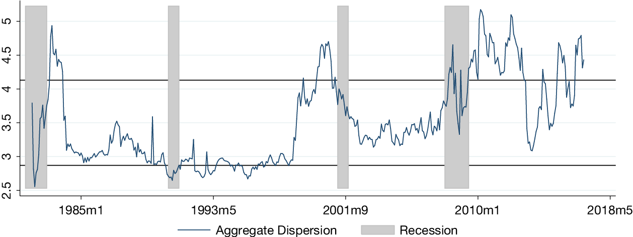
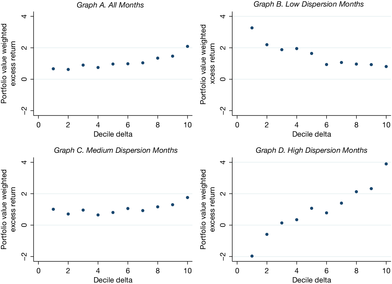


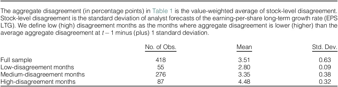
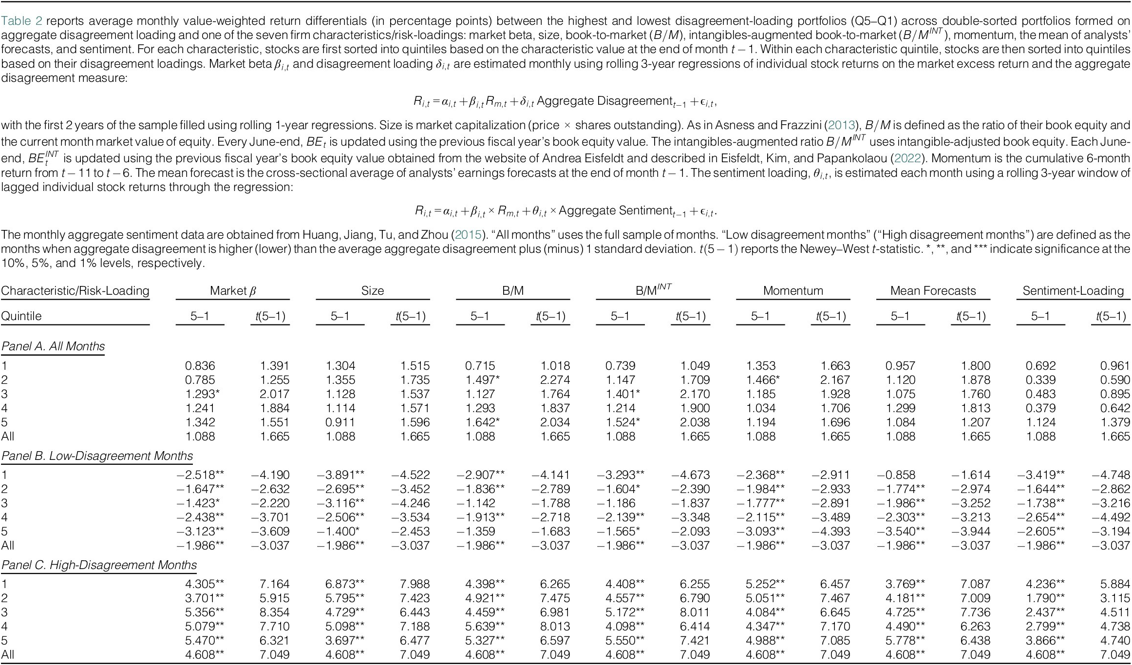
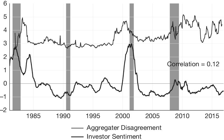
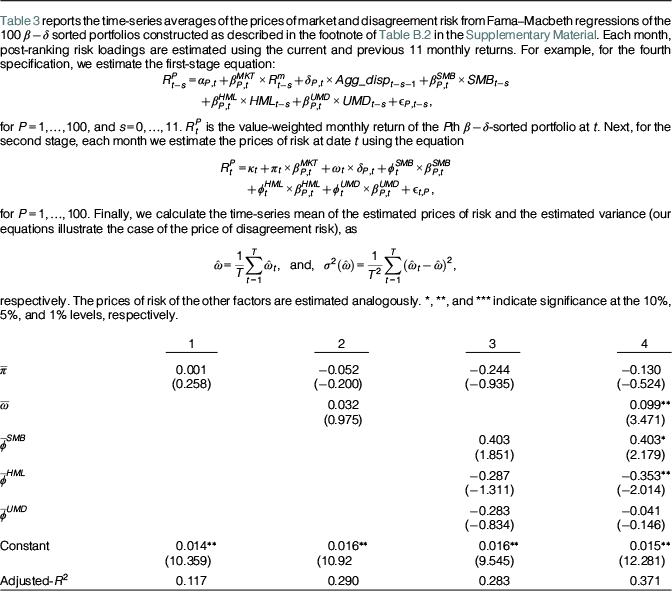

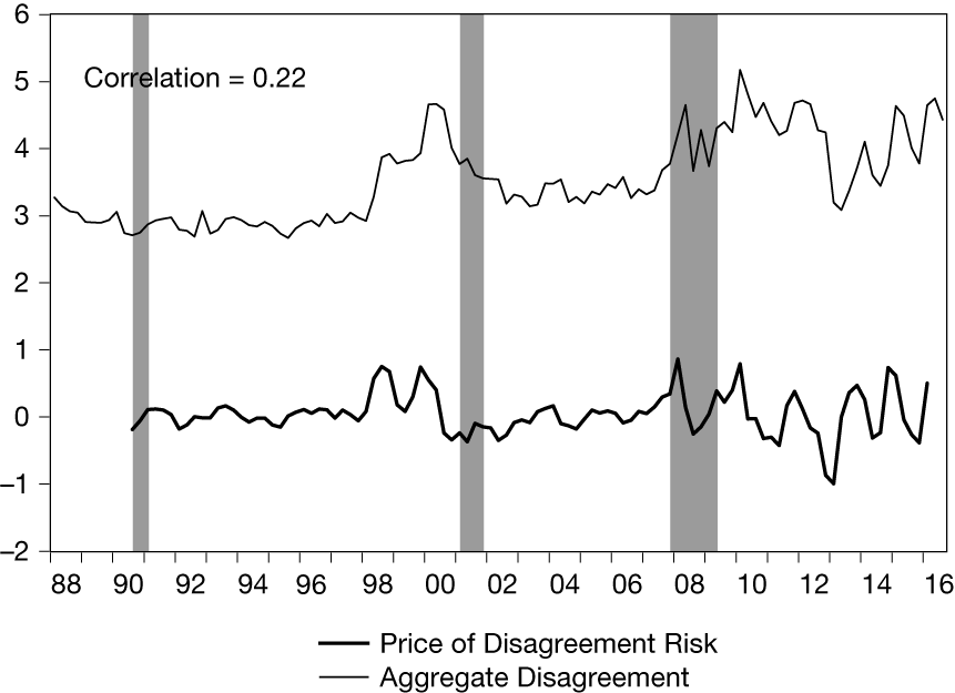


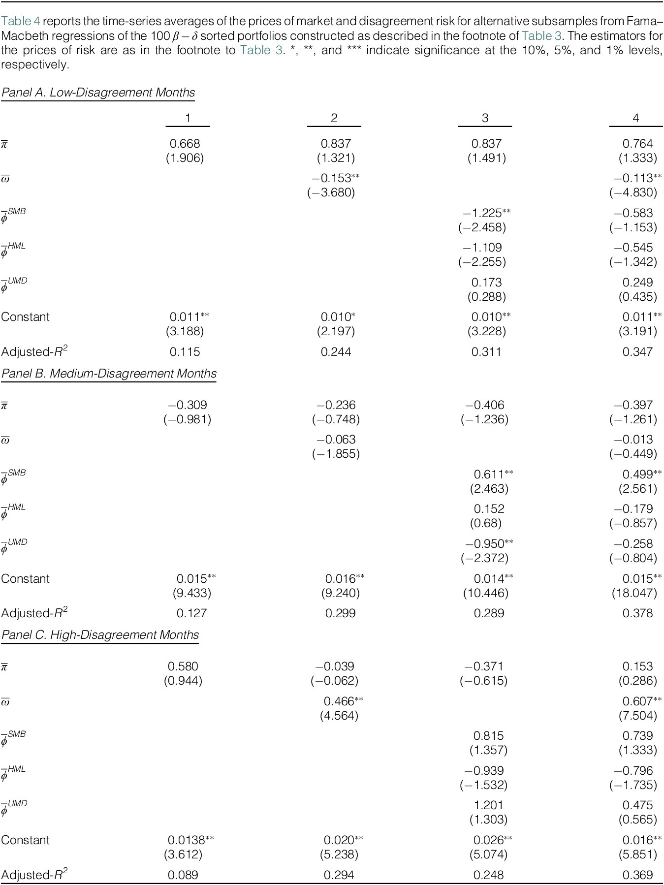

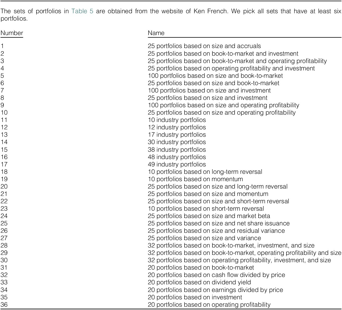



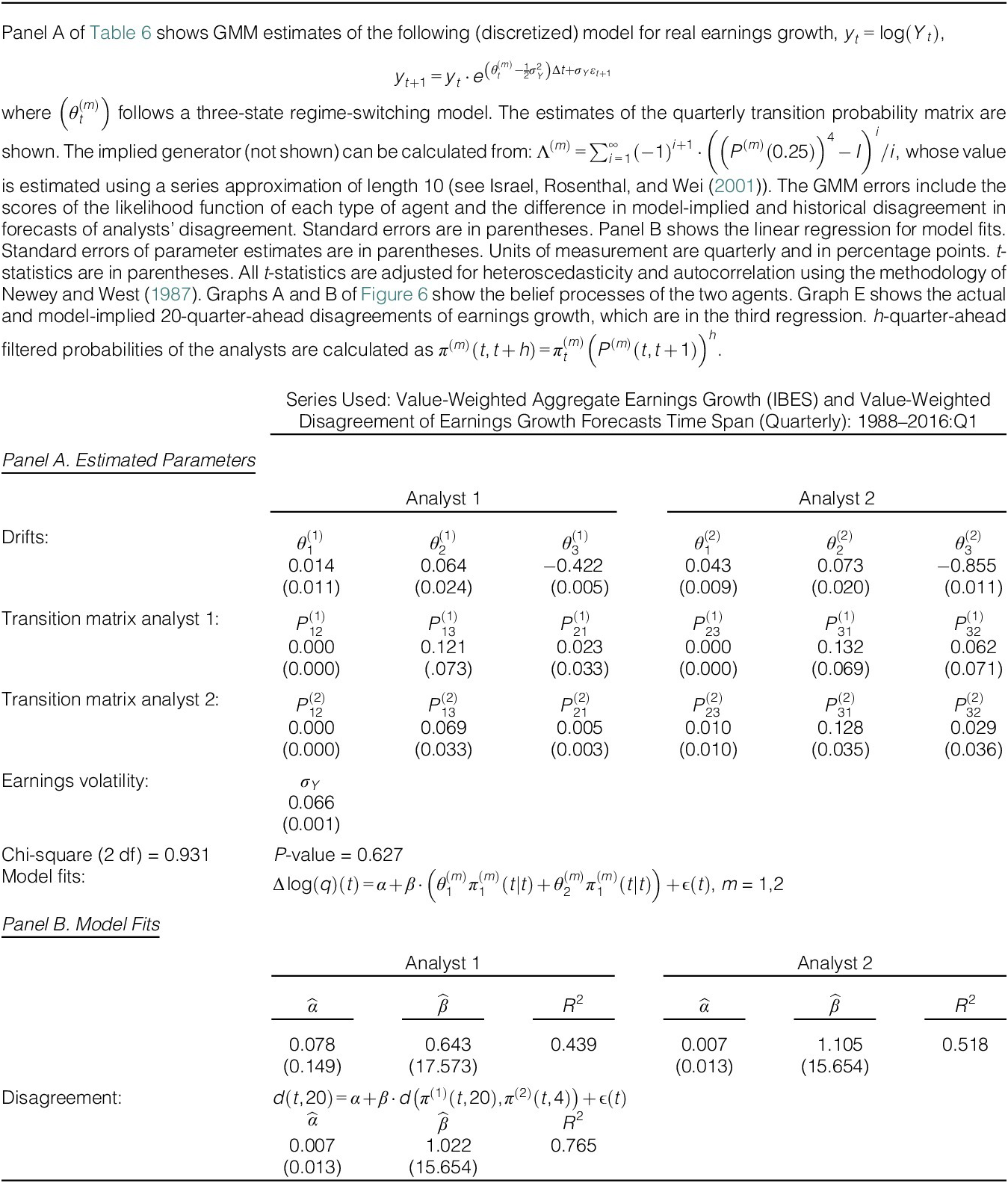
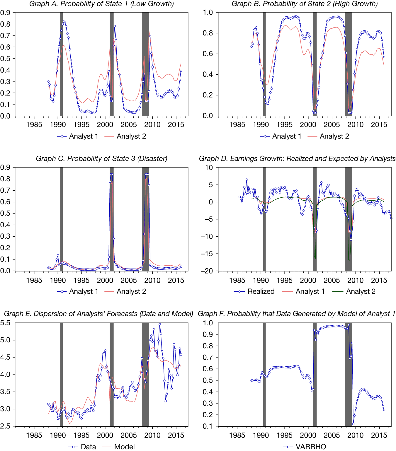


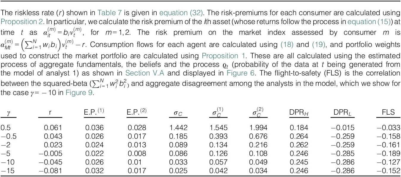
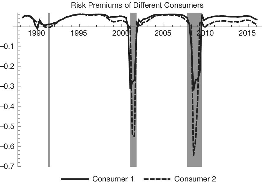


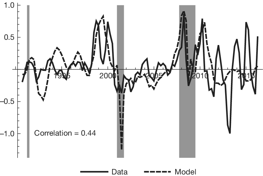
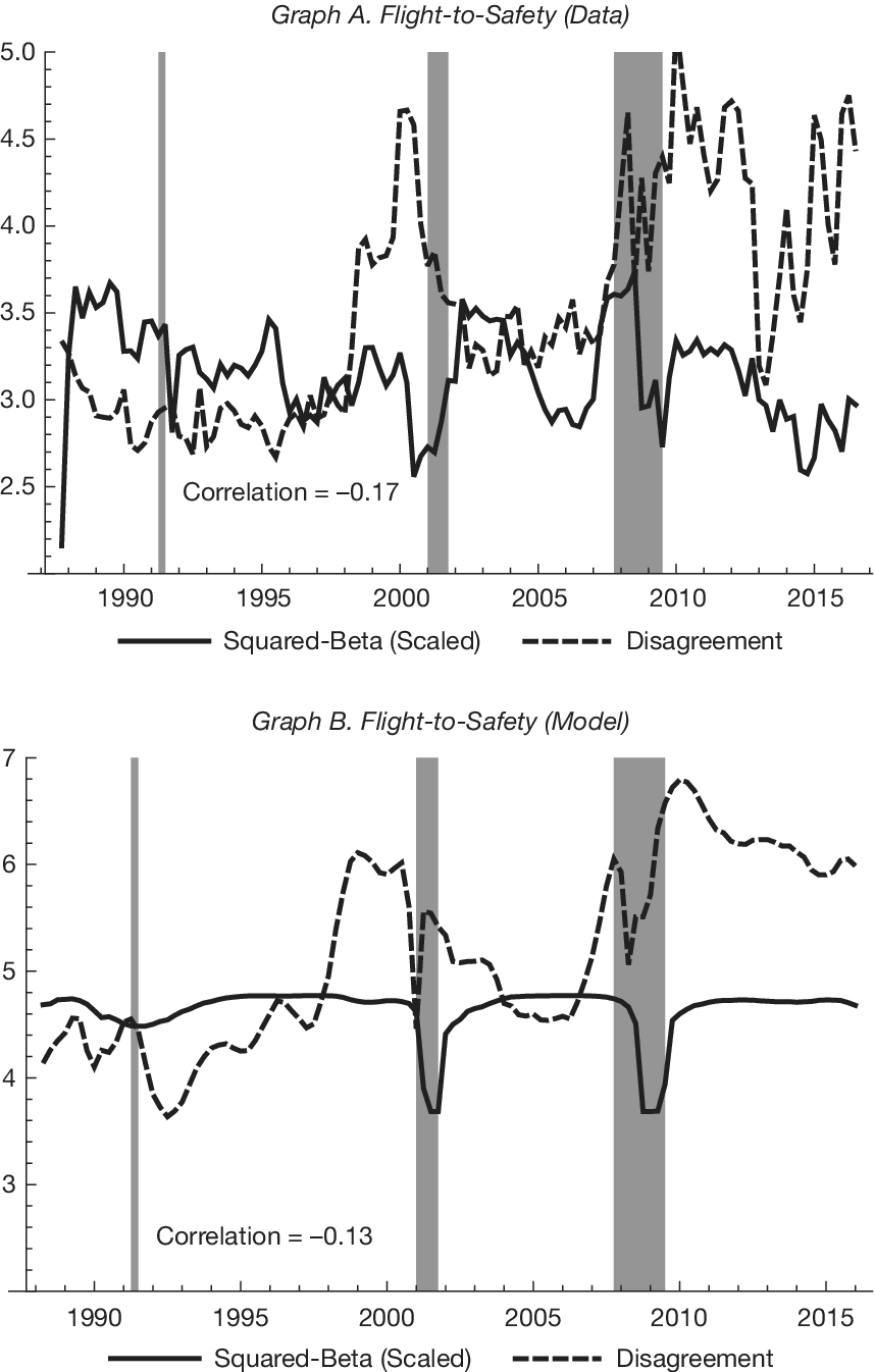


 Open access

