



1 Problem and main results
Let
 $N\geq 1$
and
 $2^*$
be the critical Sobolev exponent defined by
 $2^*=+\infty $
if
 $N=1$
or
 ${N=2}$
,
 $2^*=\frac {2N}{N-2}$
if
 $N\geq 3$
. Let
 $p\in (2,2^*)$
,
 $u_0\in L^\infty ({\mathbb {R}^N})\cap H^1({\mathbb {R}^N})$
and we consider the following semilinear parabolic problem (P):
 $$ \begin{align*} \text{(P)}\quad \left\{ \begin{array}{@{}rclll} \partial_tu&=&\Delta u-u+u|u|^{p-2}&\text{in}&{\mathbb {R}^N}\times (0,T_m),\\ u|_{t=0}&=&u_0&\text{in}&{\mathbb {R}^N}, \end{array} \right. \end{align*} $$
where
 $T_m$
denotes the maximal existence time in the sense of classical solution. We assume in this article that
 $T_m=\infty $
and u is a global-in-time solution of (P). The existence of such a solution is now well-known.
Let
 $\|\cdot \|_r$
be the standard
 $L^r({\mathbb {R}^N})$
-norm, and let
 $$ \begin{align*} \|u\|_{H^1}^2:=\|\nabla u\|_2^2+\|u\|_2^2,\quad u\in H^1({\mathbb {R}^N}). \end{align*} $$
Note that (P) has the unique, radially symmetric positive stationary solution w and it is known that
 $$ \begin{align} \begin{array}{l} \text{all the positive stationary solutions of (P) are the form } w(\cdot-a)\\ \text{for some } a\in{\mathbb {R}^N}, \end{array} \end{align} $$
see [Reference Berestycki and Lions1, Reference Gidas, Ni and Nirenberg8, Reference Kwong17]. This fact indicates that the set of (positive) stationary solutions are noncompact in
 $H^1({\mathbb {R}^N})$
due to the invariance under the spatial translation of (P).
By multiplying
 $\partial _tu$
to (P) and integrating over
 ${\mathbb {R}^N}$
, we have
 $$ \begin{align} \|\partial_tu(t)\|_2^2=-\frac{d}{dt}I(u(t)), \end{align} $$
where
 $$ \begin{align*} I(u)=\frac{1}{2}\|u\|_{H^1}^2-\frac{1}{p}\|u\|_p^p \end{align*} $$
is the energy functional associated with (P). This relation shows that
 $t\mapsto I(u(t))$
is nonincreasing. Particularly, it is known that
 $$ \begin{align} I(u(t))\downarrow d\geq 0 \text{ as } t\to\infty \end{align} $$
for global-in-time solution u. This fact is now well-known and we give a sketch of proof in Appendix A.2.
From the variational point of view, (1.3) together with (1.2) implies the existence of
 $t_n\to \infty $
such that
 $$ \begin{align*} \|\partial_tu(t_n)\|_2^2=-\frac{d}{dt}I(u(t_n))\to 0, \end{align*} $$
hence by using (P) again together with (1.3), we see that
 $$ \begin{align} u(t_n) \text{ is a Palais--Smale sequence of } I \text{ at level } d. \end{align} $$
Since our spatial domain is a noncompact
 ${\mathbb {R}^N}$
, we could not expect a priori Palais–Smale condition at level d for I in general. This fact suggests us that there may exist a global-in-time solution that is bounded in
 $H^1({\mathbb {R}^N})$
but the orbit
 $\{u(t);\,t>0\}$
is not relatively compact in the energy space
 $H^1({\mathbb {R}^N})$
. Particularly, there may exist a global-in-time solution of (P) of the form
 $$ \begin{align} u(\cdot,t)=w(\cdot-a(t))+o(1) \text{ in } H^1({\mathbb {R}^N}) \text{ with } |a(t)|\to\infty \end{align} $$
as
 $t\to \infty $
. The systematic analysis of the existence of such solutions are not yet delivered well. Recently, it is proved in [Reference Ishiwata14] that every global-in-time solution can be represented as a finite superposition of spatially of (P) (see Proposition 2.1 below). Particularly, we have
 $$ \begin{align} \sup_{t>0}\|u(t)\|_{H^1}<\infty \end{align} $$
for every global-in-time solution of (P). In this article, we consider more precise global-in-time asymptotics for a class of solutions of (P) via a suitable decomposition of u together with the use of the Łojasiewicz–Simon inequality [Reference Łojasiewicz19, Reference Simon21] (we call the ŁS inequality in the following).
Under the assumption of the nonnegativity and the compactness of
 $\mathop {\mathrm {supp}} u_0$
, there exist several results on the long-time asymptotics of u. We here cite the results of Cortazar–del Pino–Elgueta [Reference Cortazar, del Pino and Elgueta5]. The method used in [Reference Cortazar, del Pino and Elgueta5] is based on the analysis of the structure of the kernel of
 $(d^2I)_w$
, the Hessian operator of I around w, which gives an inequality controlling the spatial translation.
Proposition 1.1 [Reference Cortazar, del Pino and Elgueta5, Theorem 1.1]
Let
 $u_0\in H^1({\mathbb {R}^N})\cap C({\mathbb {R}^N})$
be a nonnegative and compactly supported initial data which gives a global-in-time solution u of (P). Then, either
 $u(\cdot ,t)$
goes to zero in
 $H^1$
-sense as
 $t\to +\infty $
or there exists a positive stationary solution W of (P) such that
 $$ \begin{align*} \lim_{t\to\infty}\|u(t)-W\|_{H^1({\mathbb {R}^N})}=0. \end{align*} $$
As for the existence of solutions to the latter behavior, it is also proved in [Reference Cortazar, del Pino and Elgueta5]
Proposition 1.2 [Reference Cortazar, del Pino and Elgueta5, Theorem 1.2]
Given
 $\psi \in H^1({\mathbb {R}^N})\cap C({\mathbb {R}^N})$
, compactly supported, nonnegative, and not identically zero, there exists a unique number
 $\lambda _0>0$
such that the solution of (P) for
 $u_0=\lambda _0\psi $
converges as
 $t\to \infty $
to a positive stationary solution W of (P). Moreover, for
 $u_0=\lambda \psi $
, we have that the solution goes to zero in
 $H^1$
-sense if
 $\lambda <\lambda _0$
and blows up in finite time if
 $\lambda>\lambda _0$
. The number
 $\lambda _0$
depends continuously on
 $\psi $
in the
 $H^1$
-norm.
Note that
 $W(\cdot )=w(\cdot -a)$
for some
 $a\in {\mathbb {R}^N}$
in view of (1.1). There are similar results of this type(see also Chill–Jendoubi [Reference Chill and Jendoubi4] and Feireisl–Petzeltova [Reference Feireisl and Petzeltova7]). The method of Chill–Jendoubi [Reference Chill and Jendoubi4] relied on the Łojasiewicz–Simon inequality, which needs the analysis of the structure of
 $\ker (d^2I)_w$
. Feireisl–Petzeltová [Reference Feireisl and Petzeltova7] use the argument given by Zelenyak which also needs the analysis of
 $\ker (d^2I)_w$
. Also, in [Reference Busca, Jendoubi and Poláčik2], the asymptotics of solutions emanating from
 $u_0$
not necessarily having a compact support for the semilinear parabolic equation
 $\partial _t u-\Delta u=f(u)$
on the whole
 ${\mathbb {R}^N}$
with f a
 $C^1$
-function satisfying
 $f(0)=0$
and
 $f'(0)<0$
is considered. Their result is that if nonnegative
 $u_0$
decays exponentially to zero and if
 $\lim _{|x|\to \infty }u(t,x)=0$
uniformly in
 $t\geq 0$
, then
 $u(t,\cdot )$
converges either to zero or to a positive solution of the corresponding stationary problem strongly in
 $H^1({\mathbb {R}^N})$
as
 $t\to \infty $
.
The proof of Proposition 1.1 consists of two steps (arguments in [Reference Chill and Jendoubi4, Reference Feireisl and Petzeltova7] are much the same). First, they prove that u converges to a positive stationary solution along some time sequence, namely, the existence of
 $(t_n)$
with
 $t_n\to \infty $
as
 $n\to \infty $
and a positive stationary solution W such that
 $$ \begin{align} u(t_n)\to W \text{ in } H^1({\mathbb {R}^N}) \end{align} $$
as
 $n\to \infty $
. In this step, the nonnegativity and the compactness of
 $\mathop {\mathrm {supp}} u_0$
is needed. Then next they show that the convergence occurs along every time sequence, namely,
 $u(t)\to W$
in
 $H^1({\mathbb {R}^N})$
as
 $t\to \infty $
by using the structure of
 $\ker (d^2I)_W$
. These results ensure that under the assumption of nonnegativity and the the compactness of
 $\mathop {\mathrm {supp}} u_0$
, solutions do not behave as in (1.5).
In this article, we remove the assumption of the nonnegativity of u and the compactness of the support of
 $u_0$
. Let
 $$ \begin{align*} d_\infty:=I(w)(=I(w(\cdot-a))) \end{align*} $$
which is the ground state energy level. The fact
 $d_\infty>0$
is well-known.
Our main result reads as follows.
Theorem 1.1 Let u be a global-in-time solution of (P) with
 $u_0\in H^1({\mathbb {R}^N})\cap L^\infty ({\mathbb {R}^N})$
satisfying
 $$ \begin{align} &I(u(t))\downarrow d\in [0,d_\infty] \text{ as } t\to\infty \end{align} $$
(recall that
 $d_\infty>0$
). Then, the following holds:
(a) If
 $d<d_\infty $
, then
 $d=0$
and
 $u(t)\to 0$
in
 $H^1({\mathbb {R}^N})$
as
 $t\to \infty $
.
(b) If
 $d=d_\infty $
, then there exist
 $T>0$
,
 $a\in C^1([T,\infty );{\mathbb {R}^N})$
,
 $a_\infty \in {\mathbb {R}^N}$
,
 $r\in C^1([T,\infty );H^1({\mathbb {R}^N}))$
,
 $C>0$
, and
 $\delta>0$
which satisfy
 $$ \begin{align} &u(\cdot,t)=w(\cdot-a(t))+r(\cdot,t),\quad t\geq T,\notag\\&|I(u(t))-d_\infty|+|a(t)-a_\infty|+ \|r(t)\|_2\leq C(I(u_0)-d_\infty)^{\frac{1}{2}} e^{-\delta t},\quad t>T, \end{align} $$
 $$ \begin{align}&\|\nabla r(t)\|_2\leq C(I(u_0)-d_\infty)^{\frac{1}{4}} e^{-\delta t},\quad t>T. \end{align} $$
Particularly, there holds
 $$ \begin{align*} \|u(t)-w(\cdot-a_\infty)\|_{H^1}\to 0 \text{ in } H^1({\mathbb {R}^N}) \end{align*} $$
as
 $t\to \infty $
.
Note that this theorem includes Proposition 1.1 (and those in [Reference Chill and Jendoubi4, Reference Feireisl and Petzeltova7]), since solutions in these papers all satisfy (1.6) and (1.8). Indeed, as for (1.8), in [Reference Cortazar, del Pino and Elgueta5] (and in [Reference Chill and Jendoubi4, Reference Feireisl and Petzeltova7]), the existence of
 $(t_n)$
which satisfies (1.7) is established in view of the nonnegativity and the compactness of
 $\mathop {\mathrm {supp}} u_0$
, which gives
 $$ \begin{align*} u(\cdot,t_n)\to W(\cdot)=w(\cdot-a) \end{align*} $$
as
 $n\to \infty $
for some
 $a\in {\mathbb {R}^N}$
. This gives
 $$ \begin{align*} I(u(t))\downarrow I(W)=I(w(\cdot-a))=d_\infty \text{ as } t\to\infty, \end{align*} $$
namely, (1.8) and thus our theorem yields the conclusion of Proposition 1.1. Also, Proposition 1.2 shows that a solution emanating from
 $u_0=\lambda _0\psi $
(respectively,
 $u_0=\lambda \psi $
for
 $0<\lambda <\lambda _0$
) behaves as in (b) (respectively, (a)) in Theorem 1.1.
Also, we can find
 $u_0$
which is not covered by the known results above and satisfies the assumptions in Theorem 1.1.
Lemma 1.1 There exists a nonnegative function with noncompact support
 $u_0\in H^1({\mathbb {R}^N})\cap L^\infty ({\mathbb {R}^N})$
such that
 $I(u_0)\in (d_\infty ,2d_\infty )$
and satisfies the assumption of Theorem 1.1.
The proof is based on the combination of somewhat known argument including the potential-well type argument [Reference Ibrahim, Jrad, Majdoub and Saanouni10–Reference Ishiwata12, Reference Ishiwata and Suzuki16, Reference Payne and Sattinger20, Reference Tan22] (see Appendix A.1).
We here give a comment on the critical case
 $\partial _tu=\Delta u+u|u|^{2^*-2}$
. In this case, different from (P), the equation is invariant under the dilation
 $u(x,t)\mapsto \lambda ^{\frac {N-2}{2}}u(\lambda ^2 x,\lambda t)$
together with spatial translation. In this case, we have to consider the effect of dilation on the noncompactness of the orbit in addition to spatial translation, namely, in the critical case, there may appear a concentration solution due to the dilation invariance. Such solutions tend to
 $0$
in
 $L^2$
. On the other hand, in this article, we only treat the effect of spatial translation on the noncompactness of the orbit based on the
 $L^2$
-framework (see, e.g., Proposition 2.3). Hence, our framework in this article cannot capture the concentration phenomena which may appear as a global-in-time behavior of global-in-time solutions for the critical case. The detailed treatment of the critical case in the spirit of this article may be an interesting open problem. See, e.g., [Reference Du6, Reference Ikehata, Ishiwata and Suzuki11, Reference Ishiwata and Suzuki16, Reference Tan22] and the references therein for the possible concentration phenomena in the critical case.
In the proof of our main result, under the assumption (1.5) together with (1.6) and (1.8), we have the following key inequality (see (3.13)) which relates the motion of the center of the mass
 $a(t)$
and the initial energy
 $I(u_0)$
:
 $$ \begin{align*} |a(t)-a(T)| \leq C(I(u_0)-d_\infty)^{\frac{1}{2}}, \end{align*} $$
where T is a time appears in Theorem 1.1. This immediately shows that
 $a(t)$
is bounded as
 $t\to \infty $
if
 $I(u_0)<\infty $
. Thus, all solutions which satisfy the assumption of Theorem 1.1 cannot escape away toward the spatial infinity.
To prove Theorem 1.1, we rely on the Łojasiewicz–Simon inequality (see Lemma 2.4) and the profile decomposition of global-in-time solutions (see Proposition 2.1) together with the decomposition of u along the continuum of stationary solutions
 $$ \begin{align} E:=\{w(\cdot-a);\,a\in{\mathbb {R}^N}\} \end{align} $$
(see Proposition 2.3), where w is the unique, radially symmetric positive stationary solution of (P).
Notation
For a function
 $f(x)$
with
 $x\in {\mathbb {R}^N}$
,
 $\frac {\partial f(x)}{\partial x_j}$
and
 $\frac {\partial ^2 f(x)}{\partial x_k\partial x_j}$
are denoted by
 $\partial _jf$
,
 $\partial _{kj}^2f$
, respectively (
 $j,k=1,\dots ,N$
). For
 $a\in {\mathbb {R}^N}$
,
 $f_a:=f(\cdot -a)$
. The
 $L^2({\mathbb {R}^N})$
-inner product is denoted by
 $(\cdot ,\cdot )_2$
. The unique, radially symmetric positive stationary solution of (P) is represented by w and
 $d_\infty :=I(w)$
(the ground energy level).
2 Preliminaries
On the asymptotic bounds
We use several types of decompositions of u to prove Theorem 1.1. First, we review the profile decomposition of general global-in-time solutions for (P) which states that every global-in-time solution can be represented as a superposition of spatially translated stationary solutions of (P).
Proposition 2.1 (Asymptotics for general global-in-time solutions [Reference Ishiwata14])
Let u be an arbitrary global-in-time solution of (P). Then, for any
 $(t_n)$
with
 $t_n\to \infty $
as
 $n\to \infty $
, there exist
 $M\in {\mathbb {N}}$
, a family of stationary solutions
 $(W_j)_{j=1}^M$
of (P),
 $(a_{n,j})_{n\in {\mathbb {N}}}\subset {\mathbb {R}^N}$
(
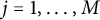 $j=1,\dots ,M$
) such that
 $$ \begin{align} &u(t_n)=\sum_{j=1}^M W_j(\cdot-a_{n,j})+o(1) \text{ in } H^1({\mathbb {R}^N}), \end{align} $$
 $$ \begin{align} &|a_{n,i}-a_{n,j}|\to\infty \text{ for } i,j\in\{1,\dots,M\} \text{ with } i\neq j, \notag\\&u(\cdot+a_{n,j},t_n)\rightharpoonup W_j \text{ weakly in } H^1({\mathbb {R}^N}) \text{ for } j\in\{1,\dots,M\}, \notag\\& \|u(t_n)\|_{H^1}^2= \sum_{j=1}^M\|W_j\|_{H^1}^2+o(1), \quad \|u(t_n)\|_p^p= \sum_{j=1}^M\|W_j\|_p^p+o(1) \end{align} $$
as
 $n\to \infty $
passing to a subsequence if necessary. Particularly, the orbit of u is bounded in
 $H^1({\mathbb {R}^N})$
.
Note that it may happen that
 $W_j=0$
(which is also a stationary solution) in the above.
The uniform boundedness (1.6) of u in
 $H^1({\mathbb {R}^N})$
is assured by Proposition 2.1. Under (1.6) which is assured by Proposition 2.1, we have the
 $L^\infty $
-global bounds.
Lemma 2.1 For any global-in-time solution u, there holds
 $$ \begin{align} M:=\sup_{t>0}\|u(t)\|_\infty<\infty. \end{align} $$
Since we treat the subcritical nonlinearity, this lemma could be proved via a standard argument (see, e.g., [Reference Cazenave and Lions3]). We give a sketch of the proof for the case
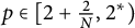 ${p\in [2+\frac {2}{N},2^*)}$
in Appendix A.3 based on the argument in [Reference Ishiwata13].
We also need the decay of
 $\|\partial _t u(t)\|_2$
to have the estimate on
 $\|u(t)- w(\cdot -a(t))\|_{H^1}$
.
Lemma 2.2 Let u be a global-in-time solution of (P). Then
 $$ \begin{align} \|\partial_tu(t)\|_2\to 0 \text{ as } t\to\infty. \end{align} $$
Proof of Lemma 2.2
The relation (2.4) in the case
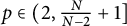 $p\in (2,\frac {N}{N-2}+1]$
is proved in [Reference Feireisl and Petzeltova7, Lemma 3.1], thus we assume
 $p\in (\frac {N}{N-2}+1,2^*)$
in the following. Note that since
 $2+\frac {2}{N}<\frac {N}{N-2}+1$
, we have the
 $L^\infty $
-global bounds (2.3) by Lemma 2.1.
Let
 $(t_n)$
be an arbitrary time-sequence satisfying
 $t_n\to \infty $
as
 $n\to \infty $
. Let
 $u_n(s):=u(t_n+s)$
and
 $v_n(s):=\partial _t u_n(s)$
, where
 $s\in [-1,0]$
. Then, (1.2) and (1.3) imply that
 $$ \begin{align*} \int_{s=-1}^{s=0}\|v_n(s)\|_2^2 =I(u_n(-1))-I(u_n(0))\to d-d=0, \end{align*} $$
thus there exists
 $s_0\in [-1,0]$
such that
 $$ \begin{align} \|v_n(s_0)\|_2^2\to 0 \text{ as } n\to\infty \end{align} $$
by taking a subsequence if necessary.
By differentiating (P) with respect to the time variable, we have
 $$ \begin{align*} \partial_sv_n=\Delta v_n-v_n+(p-1)|u_n|^{p-2}v_n, \end{align*} $$
which implies
 $$ \begin{align*} \frac{d}{ds}\frac{1}{2}\|v_n(s)\|_2^2 \leq (p-1)\int |u_n|^{p-2}v_n^2 \leq (p-1)M^{p-2}\|v_n(s)\|_2^2 \end{align*} $$
by multiplying
 $v_n$
and integrating over
 ${\mathbb {R}^N}$
and we use (2.3) in the last inequality. Then there holds
 $$ \begin{align*} \|v_n(0)\|_2^2\leq\|v_n(s_0)\|_2^2e^{C|s_0|}, \end{align*} $$
for some
 $C>0$
, which together with (2.5) yields
 $$ \begin{align*} \|\partial_t u(t_n)\|_2^2=\|v_n(0)\|_2^2\to 0 \text{ as } n\to\infty, \end{align*} $$
which implies (2.4).
A decomposition of the dynamics
We need a decomposition of u under the assumption (1.8). To introduce this decomposition, we recall two basic facts.
Proposition 2.2 (The implicit function theorem)
Let
 $F\in C^1({\mathbb {R}}_+\times {\mathbb {R}}^N:{\mathbb {R}^N})$
and
 $(t_0,a_0)\in {\mathbb {R}}_+\times {\mathbb {R}^N}$
be a point satisfying
 $F(t_0,a_0)=0$
and
 $$ \begin{align*} \det(\partial_kF_j(t_0,a_0))\neq 0. \end{align*} $$
Then, there exists a neighborhood
 $U\subset {\mathbb {R}}_+$
of
 $t_0$
,
 $V\subset {\mathbb {R}^N}$
of
 $a_0$
, a unique
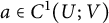 $a\in C^1(U;V)$
such that
 $$ \begin{align*} &F(t,a(t))=0,\quad (t,a)\in U\times V,\\ &\dot{a}(t)=-\left(\partial_k F_j(t,a(t))\right)^{-1}\partial_tF(t,a(t)). \end{align*} $$
Lemma 2.3 Let w be a radially symmetric function. Then, there holds
 $$ \begin{align} (\partial_jw,\partial_kw)_2=\|\partial_1w\|_2^2\delta_{jk}. \end{align} $$
Now we introduce the following decomposition for u which plays a crucial role for Theorem 1.1. Let us recall that w is the unique, positive, radially symmetric stationary solution of (P),
 $w_a(\cdot ):=w(\cdot -a)$
and
 $d_\infty :=I(w)$
.
Proposition 2.3 Let u be a global-in-time solution of (P) satisfying
 $$ \begin{align} I(u(t))\downarrow d_\infty \text{ as } t\to\infty. \end{align} $$
Then, there exist
 $T>0$
,
 $a\in C^1([T,\infty );{\mathbb {R}^N})$
, and
 $r\in C^1([T,\infty );H^1({\mathbb {R}^N}))$
which satisfy
 $$ \begin{align*} u(t)=w_{a(t)}+r(t) \text{ with } r(t)\to 0\text{ in }H^1({\mathbb {R}^N})\text{ as }t\to\infty \end{align*} $$
and
 $$ \begin{align} (r(t),(\partial_jw)_{a(t)})_2=0,\quad j=1,\dots,N \end{align} $$
for
 $t>T$
. Particularly, we have
 $$ \begin{align} (\partial_tr(t),(\partial_jw)_{a(t)})_2=\sum_{k=1}^N\dot{a}_k(t)(r(t), (\partial_{kj}^2w)_{a(t)})_2,\quad t>T. \end{align} $$
Proof of Proposition 2.3
Let
 $u(t)$
be a global-in-time solution satisfying (2.7). For any
 $(t_n)$
with
 $t_n\to \infty $
as
 $n\to \infty $
, by (2.2) in Proposition 2.1, we see that there exists
 $M\in {\mathbb {N}}$
such that
 $$ \begin{align*} I(u(t_n))=\sum_{j=1}^M\left(\frac{1}{2}\|W_j\|_{H^1}^2-\frac{1}{p} \|W_j\|_p^p\right)+o(1) \end{align*} $$
along subsequence of
 $(t_n)$
. This relation with (2.7) imply that
 $M=1$
. Moreover,
 $W_1$
is a stationary solution of (P) with
 $I(W_1)=d_\infty $
, we have
 $W_1=w_a$
for some
 $a\in {\mathbb {R}^N}$
in view of (1.1). Particularly, for some
 $(a_n)\subset {\mathbb {R}^N}$
and along some subsequence, we obtain
 $$ \begin{align*} u(t_n)= w_{a_n}+o(1)\text{ in }H^1({\mathbb {R}^N}) \end{align*} $$
by (2.1). This convergence yields
 $$ \begin{align} d_{H^1}(u(t),E)\to 0\text{ as }t\to\infty, \end{align} $$
where E is the continuum of stationary solutions
 $$ \begin{align*} E:=\{w_a;\,a\in{\mathbb {R}^N}\} \end{align*} $$
and
 $d_{H^1}$
denotes the standard
 $H^1$
-metric.
Let
 $d(t,a):=\|u(t)-w_a\|_2^2$
. First, we assure the existence of a satisfying
 $$ \begin{align*} d(t):=\inf_{b\in{\mathbb {R}^N}}d(t,b)=d(t,a) \end{align*} $$
for large t. Let
 $(a_n)\subset {\mathbb {R}^N}$
be a minimizing sequence. First, we see that
 $(a_n)$
is a bounded sequence. Indeed, suppose not. Then, we have
 $$ \begin{align*} d(t) = d(t,a_n)+o(1) = \|u(t)\|_2^2-2\int u(t)w_{a_n}+\|w_{a_n}\|_2^2+o(1) \end{align*} $$
as
 $n\to \infty $
passing to a subsequence of
 $(a_n)$
if necessary. This relation together with the fact
 $w_{a_n}\rightharpoonup 0$
weakly in
 $L^2$
and
 $\|w_{a_n}\|_2=\|w\|_2$
implies
 $$ \begin{align} d(t)=\|u(t)\|_2^2+\|w\|_2^2. \end{align} $$
On the other hand, by (2.10), we see that
 $$ \begin{align*} d(t)\leq d_{H^1}(u(t),E)\leq\frac{1}{2}\|w\|_2^2\text{ as }t\to\infty, \end{align*} $$
which contradicts (2.11). Thus, there exists
 $T_1>0$
such that
 $$ \begin{align} d(t) \text{ is attained for } t>T_1. \end{align} $$
It is easy to see that
 $$ \begin{align} F_j(t,a)&:=\partial_jd(t,a) =2\int (u(t)-w_a)(\partial_j w)_a,\notag\\ \partial_kF_j(t,a)&:=\partial_{kj}^2d(t,a)= 2\left[\int (\partial_k w)_a(\partial_j w)_a -\int (u(t)-w_a)(\partial_k\partial_jw)_a\right]\notag\\ &= 2\|\partial_1w\|_2^2\delta_{kj} -\int r(t)(\partial_{kj}^2w)_a \end{align} $$
in view of Lemma 2.3. Moreover, (2.10) leads
 $\|r(t)\|_2\to 0$
as
 $t\to \infty $
, thus we have the existence of
 $T_2>0$
such that
 $$ \begin{align} \left|\int r(t)(\partial_{kj}^2w)_a\right| \leq C\|r(t)\|_2 \leq \|\partial_1w\|_2^2,\quad t>T_2. \end{align} $$
Now take for any
 $h_k$
,
 $h_j\in {\mathbb {R}}$
. Then, (2.14) and (2.13) imply the existence of
 $T_2>0$
which does not depend on
 $a\in {\mathbb {R}^N}$
such that
 $$ \begin{align*} \sum_{k,j}\partial_{kj}^2d(t,a)h_kh_j &= 2\|\partial_1w\|_2^2\sum_{k,j}\delta_{kj}h_kh_j -\|r(t)\|_2\sum_{k,j}\|\partial_{kj}^2w\|_2h_kh_j\\ &\geq 2\|\partial_1w\|_2^2|h|^2 -\|\partial_1w\|_2^2|h|^2 \geq \|\partial_1w\|_2^2|h|^2, \end{align*} $$
where we used the equivalence of norms on finite-dimensional vector space, thus
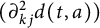 $(\partial _{kj}^2d(t,a))$
is positive definite, which implies
 $d(t,a)$
is convex in
 $a\in {\mathbb {R}^N}$
for each
 $t>T$
. This together with (2.12) implies that, for each
 $t_0>\max (T_1,T_2)$
, there exists a unique minimum point
 $a_0$
of
 $d(t_0,a)$
.
Now we apply the implicit function theorem. Note that for any
 $(t,a)\in {\mathbb {R}}\times {\mathbb {R}}$
, we have, by (2.13) and
 $\|r(t)\|_2\to 0$
as
 $t\to \infty $
,
 $$ \begin{align} \det (\partial_kF_j(t,a))\geq \|\partial_1 w\|_2^{2N},\quad t>T_3 \end{align} $$
holds for some
 $T_3$
.
Let
 $T:=\max (T_1,T_2,T_3)+1$
and take any
 $t_0>T$
. Let
 $a_0$
be the corresponding minimizer of
 $d(t_0,\cdot )$
, which implies
 $$ \begin{align*} F_j(t_0,a_0)=0,\quad j=1,\dots,N. \end{align*} $$
Then by the implicit function theorem together with (2.15), we have a neighborhood
 $U(\subset [T_3,\infty ))$
of
 $t_0$
, a neighborhood
 $V (\subset {\mathbb {R}}^N)$
of
 $a_0$
, a unique function
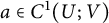 $a\in C^1(U;V)$
satisfying
 $$ \begin{align} F_j(t,a(t))=0,\quad t\in U,\quad j=1,\dots,N. \end{align} $$
The uniqueness of the minimizer of
 $d(t_0,\cdot )$
for
 $t_0>T$
allows us to prolong
 $a(t)$
on
 $[T,\infty )$
and
 $a\in C^1([T,\infty ))$
is a unique solution of (2.16).
Then,
 $r(t):=u(t)-w_{a(t)}$
satisfies
 $$ \begin{align*} 0=F_j(t,a(t))=\int (u(t)-w_{a(t)})(\partial_j w)_{a(t)} =\int r(t)(\partial_j w)_{a(t)} \end{align*} $$
in view of (2.16), thus we have (2.8).
Note that u and w are smooth functions and
 $a\in C^1$
, we see that r is differentiable in t. Then, by differentiating (2.8) in t, we obtain
 $$ \begin{align*} (\partial_tr(t),(\partial_jw)_{a(t)})_2+\left(r(t),\sum_{k=1}^N(\partial_{kj}^2w)_{a(t)} (-\dot{a}_k(t))\right)_2=0, \end{align*} $$
which implies (2.9).
On the Łojasiewicz–Simon inequality
Let
 $$ \begin{align*} Mv:=\Delta v-v+v|v|^{p-2},\quad v\in H^1({\mathbb {R}}^N). \end{align*} $$
Here, we recall Lemma 2.8 in [Reference Chill and Jendoubi4].
Lemma 2.4 (The Łojasiewicz–Simon inequality)
Let W be a positive stationary solution of (P). Then, there exists
 $\sigma $
,
 $C>0$
such that for every
 $v\in H^1({\mathbb {R}^N})$
with
 ${\|v-W\|_{H^1}<\sigma }$
, there holds
 $$ \begin{align*} \left| I(v)-I(W) \right|{}^{\frac{1}{2}} \leq C\|Mv\|_{H^{-1}}. \end{align*} $$
It is natural to guess that, the situation around
 $w_a$
is the same as the situation around
 $w_0=w$
since the functional I is invariant under the spatial translation. Indeed, we can show the following:
Lemma 2.5 Let w be a positive radially symmetric stationary solution of (P). Then there exists
 $\sigma $
,
 $C>0$
such that for every
 $a\in {\mathbb {R}^N}$
and
 $v\in H^1({\mathbb {R}^N})$
with
 $\|v-w_a\|_{H^1}<\sigma $
, there holds
 $$ \begin{align*} \left| I(v)-d_\infty \right|{}^{\frac{1}{2}} \leq C\|Mv\|_{H^{-1}} \leq C\|Mv\|_2, \end{align*} $$
where
 $d_\infty :=I(w)$
.
Proof of Lemma 2.5
Let
 $\sigma $
, C be numbers given in Lemma 2.4. Take any
 $a\in {\mathbb {R}^N}$
and
 $v\in H^1$
with
 $\|v-w_a\|_{H^1}<\sigma $
. Then, we have
 $\|v_{-a}-w\|_{H^1}<\sigma $
, hence by Lemma 2.4, we obtain
 $$ \begin{align*} \left| I(v_{-a})-d_\infty \right|{}^{\frac{1}{2}} \leq C\|Mv_{-a}\|_{H^{-1}}. \end{align*} $$
By noting
 $$ \begin{align*} I(v_{-a})=I(v)\text{ and }\|Mv_{-a}\|_{H^{-1}} =\|Mv\|_{H^{-1}}, \end{align*} $$
we have the conclusion for
 $H^{-1}$
-norm. The result for
 $L^2$
-norm is easy.
It is clear that Lemma 2.5 yields the following.
Corollary 2.1 Let w be a positive radially symmetric stationary solution of (P) and
 $\sigma $
, C be numbers in Lemma 2.5. Assume that v satisfies
 $\|v-w_a\|_{H^1}<\sigma $
for some
 $a\in {\mathbb {R}^N}$
. Then there holds
 $$ \begin{align*} \left| I(v)-d_\infty \right|{}^{\frac{1}{2}} \leq C\|Mv\|_2. \end{align*} $$
3 Proof of Theorem 1.1
For the proof of Theorem 1.1, we first show the following proposition.
Proposition 3.1 Let u be a global-in-time solution of (P) satisfying (2.7). Then there exists
 $C_1>0$
such that
 $$ \begin{align} |\dot{a}(t)|\leq C_1\|\partial_t u(t)\|_2,\quad t\geq T, \end{align} $$
where T is the time appeared in Proposition 2.3.
Proof of Proposition 3.1
By the assumption on u, we can use Proposition 2.3 and we have the decomposition for u in Proposition 2.3. Then we have
 $$ \begin{align*} \partial_t u(t)=\sum_{k=1}^N(\partial_kw)_{a(t)}(-\dot{a}_k(t))+\partial_tr(t) \end{align*} $$
for any t with
 $t\geq T$
. This implies, for
 $j=1,\dots , N$
,
 $$ \begin{align*} (\partial_t u(t),(\partial_jw)_{a(t)})_2 &= -\sum_{k=1}^N\dot{a}_k(t)((\partial_kw)_{a(t)},(\partial_jw)_{a(t)})_2 +(\partial_tr,(\partial_jw)_{a(t)})_2\\ &= -\sum_{k=1}^N\dot{a}_k(t)[(\partial_kw,\partial_jw)_2+ (r(t),(\partial_{kj}^2w)_{a(t)})_2]\\ &= -\sum_{k=1}^N\dot{a}_k(t)[\|\partial_1w\|_2^2\delta_{kj}+ (r(t),(\partial_{kj}^2w)_{a(t)})_2], \end{align*} $$
where we used (2.9) in the second equality and (2.6) in the last equality. Then we have
 $$ \begin{align} \sum_{k=1}^N\alpha_{kj}(t)\dot{a}_k(t) = \beta_j(t), \end{align} $$
where
 $$ \begin{align*} \alpha_{kj}(t) :=-\|\partial_1w\|_2^2\delta_{kj}-(r(t),(\partial_{kj}w)_{a(t)})_2,\quad \beta_j(t) := (\partial_t u(t),(\partial_jw)_{a(t)})_2. \end{align*} $$
Let
 $A(t):=(\alpha _{kj}(t))$
. Since
 $\|r(t)\|_2\to 0$
as
 $t\to \infty $
by Proposition 2.3, we have
 $$ \begin{align} \alpha_{kj}(t)=\|\partial_1w\|_2^2\delta_{kj}+o(1), \end{align} $$
thus
 $A(t)^{-1}$
is well-defined for large t and (3.2) gives
 $$ \begin{align} \dot{a}_k(t)=\sum_{j=1}^N(A(t)^{-1})_{kj}\beta_j(t). \end{align} $$
Moreover, we see from (3.3) that
 $$ \begin{align*} (A(t)^{-1})_{kj}=\frac{1}{\|\partial_1w\|_2^2}\delta_{kj}+o(1), \end{align*} $$
thus (3.4) leads
 $$ \begin{align*} |\dot{a}_k(t)| &\leq \sum_{j=1}^N|(A(t)^{-1})_{kj}||\beta_j(t)| \leq \sum_{j=1}^N\left(\frac{1}{\|\partial_1w\|_2^2}\delta_{kj}+o(1)\right) \|\partial_jw\|_2\|\partial_tu(t)\|_2\\ &= \left[\frac{1}{\|\partial_1w\|_2}+o(1)\right]\|\partial_tu(t)\|_2, \end{align*} $$
where we used
 $\|\partial _1w\|_2=\|\partial _jw\|_2$
by the radial symmetry of w (see Lemma 2.3). This implies
 $$ \begin{align*} |\dot{a}(t)|\leq C\|\partial_tu(t)\|_2,\quad t>T, \end{align*} $$
thus we have obtained (3.1).
Proposition 3.2 (A consequence of the ŁS-inequality)
Let u be a global-in-time solution of (P) satisfying (2.7). Then there exist
 $T>0$
and
 $C_2>0$
such that
 $$ \begin{align} &\|\partial_t u(t)\|_2 \leq -C_2\frac{d}{dt}(I(u(t))-d_\infty)^{\frac{1}{2}}, \end{align} $$
 $$ \begin{align} &\frac{d}{dt} (I(u(t))-d_\infty)^{\frac{1}{2}} \leq -C_2(I(u(t))-d_\infty)^{\frac{1}{2}} \end{align} $$
for
 $t\geq T$
.
Proof of Proposition 3.2
By Proposition 2.3, taking T further large if necessary, we can assume that
 $$ \begin{align} \|u(t)-w_{a(t)}\|_{H^1}<\sigma,\quad t>T, \end{align} $$
where
 $\sigma $
is the number that appeared in Corollary 2.1. In the following, we fix such t.
Note that (1.3), (1.2), and (2.7) yield
 $$ \begin{align} I(u(t))-d_\infty\downarrow 0\text{ as }t\to\infty \end{align} $$
and
 $$ \begin{align*} \frac{d}{dt}(I(u(t))-d_\infty) = \frac{d}{dt}I(u(t))=-\|\partial_t u(t)\|_2^2\leq 0, \end{align*} $$
respectively. These relations imply
 $$ \begin{align*} -\|\partial_t u(t)\|_2^2 &= \frac{d}{dt}(I(u(t))-d_\infty) = \frac{d}{dt}[(I(u(t))-d_\infty)^{\frac{1}{2}}]^2\\ &= 2(I(u(t))-d_\infty)^{\frac{1}{2}} \frac{d}{dt}(I(u(t))-d_\infty)^{\frac{1}{2}}, \end{align*} $$
thus
 $$ \begin{align} -\frac{d}{dt}(I(u(t))-d_\infty)^{\frac{1}{2}} = \frac{1}{2} (I(u(t))-d_\infty)^{-\frac{1}{2}}\|\partial_t u(t)\|_2^2. \end{align} $$
Next we bound
 $(I(u(t))-d_\infty )^{-\frac {1}{2}}$
from below by the ŁS-inequality. The fact (3.7) allows us to use the conclusion of Corollary 2.1 with
 $v=u(t)$
, hence we have
 $$ \begin{align} (I(u(t))-d_\infty)^{\frac{1}{2}} \leq K\|Mu(t)\|_2 = K\|\partial_t u(t)\|_2 \end{align} $$
for some
 $K>0$
, where in the last equality we use
 $\partial _t u(t)=Mu(t)$
by (P). This yields
 $$ \begin{align*} \frac{1}{K\|\partial_t u(t)\|_2} \leq (I(u(t))-d_\infty)^{-\frac{1}{2}}, \end{align*} $$
which together with (3.9) gives
 $$ \begin{align*} -\frac{d}{dt}(I(u(t))-d_\infty)^{\frac{1}{2}} &= \frac{1}{2} (I(u(t))-d_\infty)^{-\frac{1}{2}}\|\partial_t u(t)\|_2^2 \geq \frac{1}{2}\frac{1}{K\|\partial_t u(t)\|_2}\|\partial_t u(t)\|_2^2\\ &= \frac{1}{2K}\|\partial_t u(t)\|_2, \end{align*} $$
thus we have (3.5).
Now we note that, by (3.9) and (3.10),
 $$ \begin{align*} -\frac{d}{dt} (I(u(t))-d_\infty)^{\frac{1}{2}} &= \frac{1}{2} (I(u(t))-d_\infty)^{-\frac{1}{2}} \|\partial_t u(t)\|_2^2\notag\\ &\geq \frac{1}{2} (I(u(t))-d_\infty)^{-\frac{1}{2}}\frac{1}{K^2} (I(u(t))-d_\infty)\\ &= \frac{1}{2K^2} (I(u(t))-d_\infty)^{\frac{1}{2}}, \end{align*} $$
hence (3.6) follows.
Now we are in the position to give a proof of Theorem 1.1.
Proof Theorem 1.1
First, we prove (a). Let u be a global-in-time solution of (P) satisfying
 $$ \begin{align} I(u(t))\downarrow d<d_\infty\text{ as }t\to\infty. \end{align} $$
By (2.2) of Proposition 2.1, we see that, for any
 $(t_n)$
with
 $t_n\to \infty $
as
 $n\to \infty $
, there exist
 $M\in {\mathbb {N}}$
and a subsequence of
 $(t_n)$
such that
 $$ \begin{align*} I(u(t_n))=\sum_{j=1}^MI(W_j) +o(1)\text{ as }n\to\infty. \end{align*} $$
Note that if there exists
 $j\in {\mathbb {N}}$
such that
 $W_j\neq 0$
, then this relation yields
 $$ \begin{align*} I(u(t_n))+o(1)\geq I(W_j)\geq I(w)=d_\infty \text{ as }n\to\infty, \end{align*} $$
since w is a ground state solution, thus
 $d\geq d_\infty $
follows. Hence under (3.11), we see that
 $W_j=0$
for any
 $j\in {\mathbb {N}}$
,
 $j\leq M$
. This together with (2.2) in Proposition 2.1 again leads
 $\|u(t_n)\|_{H^1}=o(1)$
as
 $n\to \infty $
(along subsequence). This completes the proof for case (a).
Next, we show (b). Under the assumption in (b), combining Propositions 3.2 and 3.1, we have
 $$ \begin{align} |\dot{a}(t)| \leq C_2\|\partial_t u(t)\|_2 \leq -C_2C_1\frac{d}{dt}(I(u(t))-d_\infty)^{\frac{1}{2}}. \end{align} $$
This relation with the decreasing property of
 $t\mapsto I(u(t))-d_\infty $
and (3.8) leads
 $$ \begin{align} |a(t)-a(T)| &\leq \int_0^Tds|\dot{a}(s)| \leq -C_2C_1\int_T^tds\frac{d}{ds}(I(u(t))-d_\infty)^{\frac{1}{2}}\notag\\ &= C_2C_1\left[ (I(u(T))-d_\infty)^{\frac{1}{2}} - (I(u(t))-d_\infty)^{\frac{1}{2}} \right]\notag\\ &\leq C_2C_1(I(u(0))-d_\infty)^{\frac{1}{2}}, \end{align} $$
where T is a time appears in Theorem 1.1. This shows the existence of
 $(t_n)$
with
 $t_n\to \infty $
as
 $n\to \infty $
and
 $a_\infty \in {\mathbb {R}^N}$
satisfying
 $$ \begin{align*} a(t_n)\to a_\infty\text{ as }n\to\infty.\end{align*} $$
Take any
 $s_n\to \infty $
. Without loss of generality, we assume
 $s_n\leq t_n$
. Then, by (3.12) and (3.8), we see that
 $$ \begin{align*} |a(s_n)-a_\infty| &\leq |a(s_n)-a(t_n)|+|a(t_n)-a_\infty|\\ &\leq C_2C_1[(I(u(s_n))-d_\infty)^{\frac{1}{2}}-(I(u(t_n))-d_\infty)^{\frac{1}{2}}] +|a(t_n)-a_\infty|\\ &\to 0\text{ as }n\to\infty, \end{align*} $$
which yields
 $$ \begin{align} a(t)\to a_\infty\text{ as }t\to\infty. \end{align} $$
As for the decay estimate, we start from (3.6), namely,
 $$ \begin{align*} \frac{d}{dt} (I(u(t))-d_\infty)^{\frac{1}{2}} \leq -C_2(I(u(t))-d_\infty)^{\frac{1}{2}}, \end{align*} $$
which implies
 $$ \begin{align} (I(u(t))-d_\infty)^{\frac{1}{2}} \leq (I(u(0))-d_\infty)^{\frac{1}{2}} e^{-C_2 t}. \end{align} $$
Also by integrating (3.12) and using (3.14), we have
 $$ \begin{align} |a(t)-a_\infty| &\leq \int_t^\infty ds|\dot{a}(s)| \leq \int_t^\infty ds\left[ -C_2C_1\frac{d}{ds} (I(u(s))-d_\infty)^{\frac{1}{2}}\right]\notag\\ &= C_2C_1[(I(u(t))-d_\infty)^{\frac{1}{2}} -(I(u(\infty))-d_\infty)^{\frac{1}{2}}]\notag\\ &= C_2C_1(I(u(t))-d_\infty)^{\frac{1}{2}}, \end{align} $$
where we have used the assumption
 $I(u(\infty ))-d_\infty =0$
for case (b).
Moreover, again by (3.12) with
 $(I(u(\infty ))-d_\infty )^{\frac {1}{2}}=0$
, we obtain
 $$ \begin{align} \|u(t)-w_{a_\infty}\|_2 &\leq \int_t^\infty ds\|\partial_t u(s)\|_2 \leq \int_t^\infty ds \left[ -C_2C_1\frac{d}{dt} (I(u(t))-d_\infty)^{\frac{1}{2}}\right]\notag\\ &= C_2C_1(I(u(t))-d_\infty)^{\frac{1}{2}}. \end{align} $$
By (3.15) together with (3.16) and (3.17), we obtain
 $$ \begin{align} &|I(u(t))-d_\infty|+|a(t)-a_\infty|+ \|u(t)-w(\cdot-a_\infty)\|_2\notag\\ &\leq C_3(I(u(t))-d_\infty)^{\frac{1}{2}} \leq C_3(I(u_0)-d_\infty)^{\frac{1}{2}} e^{-C_2 t},\quad t>T. \end{align} $$
Finally, we see that
 $$ \begin{align*} \partial_t u=(\Delta u-\Delta w_{a_\infty})- (u-w_{a_\infty})+u|u|^{p-2}- w_{a_\infty}|w_{a_\infty}|^{p-2}. \end{align*} $$
By multiplying
 $u-w_{a_\infty }$
to this relation and integrating over
 ${\mathbb {R}^N}$
, we see that
 $$ \begin{align*} \int \partial_t u(u-w_{a_\infty}) =&-\int |\nabla u-\nabla w_{a_\infty}|^2- \int |u-w_{a_\infty}|^2\\ &+\int (u|u|^{p-2}- w_{a_\infty}|w_{a_\infty}|^{p-2})(u-w_{a_\infty}), \end{align*} $$
hence
 $$ \begin{align} \int |\nabla u-\nabla w_{a_\infty}|^2 &\leq \left|\int \partial_t u(u-w_{a_\infty})\right| +\int |u-w_{a_\infty}|^2\notag\\ &+(p-1)\int |w_{a_\infty}+|u||^{p-2}|u-w_{a_\infty}|^2 \notag\\ &=:\mathrm{(I)}+\mathrm{(II)}+\mathrm{(III)}. \end{align} $$
Recall that, under the assumption of (b), we have Lemma 2.1, namely, the
 $L^\infty $
-global bound (2.3) and then we have
 $$ \begin{align*} \|\partial_t u(t)\|_2\to 0\text{ as }t\to\infty, \end{align*} $$
which is the conclusion of Lemma 2.2. Thus by taking T large if necessary, we can assume
 $$ \begin{align*} \|\partial_t u(t)\|_2<\frac{1}{2},\quad t>T, \end{align*} $$
which gives
 $$ \begin{align*} \mathrm{(I)}\leq \|\partial_t u(t)\|_2\|u(t)-w_{a_\infty}\|_2 \leq \frac{1}{2}\|u(t)-w_{a_\infty}\|_2. \end{align*} $$
Moreover, as for (III), again by (2.3), we see that
 $$ \begin{align*} \text{(III)}\leq (p-1)(M^{p-2}+\|w\|_\infty^{p-2}) \|u(t)-w_{a_\infty}\|_2^2. \end{align*} $$
These estimates together with (3.15), (3.17), (3.19), and the fact
 $I(u(t))\downarrow d_\infty $
yield
 $$ \begin{align*} \|\nabla u-\nabla w_{a_\infty}\|_2^2 &\leq \left(1+(p-1)(M^{p-2}+\|w\|_\infty^{p-2})\right) \|u(t)-w_{a_\infty}\|_2^2 +\frac{1}{2}\|u(t)-w_{a_\infty}\|_2\notag\\ &\leq C_4\left((I(u(t))-d_\infty) +(I(u(t))-d_\infty)^{\frac{1}{2}}\right)\notag\\ &\leq C_5(I(u(t))-d_\infty)^{\frac{1}{2}} \leq C_5(I(u(0))-d_\infty)^{\frac{1}{2}}e^{-C_2 t}, \end{align*} $$
thus follows
 $$ \begin{align} \|\nabla u-\nabla w_{a_\infty}\|_2 \leq C_5^{\frac{1}{2}}(I(u(0))-d_\infty)^{\frac{1}{4}}e^{-\frac{C_2}{2} t}. \end{align} $$
Relations (3.18) and (3.20) give (1.9) and (1.10), respectively. This completes the proof.
A Appendix
A.1 A sketch of proof of Lemma 1.1
In this section, we give a sketch of proof of Lemma 1.1.
Potential-well argument
First, we introduce the stable set and the unstable set for (P). Let
 $$ \begin{align*} J(u):=\|u\|_{H^1}^2-\|u\|_p^p \end{align*} $$
be the Nehari functional, and let
 $$ \begin{align*} W&:=\{u\in H^1({\mathbb {R}^N});\,I(u)<d_\infty,\ J(u)\geq 0\},\\ V&:=\{u\in H^1({\mathbb {R}^N});\,I(u)<d_\infty,\ J(u)< 0\}. \end{align*} $$
These sets are called the stable set and the unstable set for (P), respectively, since we have the following.
Lemma A.1 (Theorems 1.2 and 1.3 in [Reference Ishiwata, Ruf, Sani and Terraneo15])
If
 $u(t_0)\in W$
for some
 $t_0\in [0,T_m)$
, then
 $T_m=\infty $
,
 $u(t)\in W$
for
 $t\in [t_0,\infty )$
and
 $u(t)\to 0$
in
 $H^1({\mathbb {R}^N})$
as
 $t\to \infty $
.
If
 $u(t_0)\in V$
for some
 $t_0\in [0,T_m)$
, then
 $T_m<\infty $
and
 $u(t)\in V$
for
 $t\in [t_0,T_m)$
.
The basic reference for the above “potential-well” type argument is [Reference Payne and Sattinger20]. The critical case is treated, e.g., in [Reference Ikehata, Ishiwata and Suzuki11, Reference Ishiwata12, Reference Ishiwata and Suzuki16, Reference Tan22]. In [Reference Ibrahim, Jrad, Majdoub and Saanouni10], the potential-well type argument for the exponential nonlinearity in two spatial dimension case is given.
Classification of the modulus of the initial data
Now we fix a nonnegative
 $a\in H^1({\mathbb {R}^N})\cap L^\infty ({\mathbb {R}^N})$
which plays a role of the profile of an initial datum. We do not assume the compactness of
 $\mathop {\mathrm {supp}} a$
. Let
 $u_\lambda $
be a solution of (P) with
 $u_0:=\lambda a$
for
 $\lambda>0$
and we denote the maximal existence time
 $T_m$
of
 $u_\lambda $
by
 $T_m(\lambda )$
. For a above, let
 $$ \begin{align*} {\cal A}(a) &:=\{\lambda\in (0,\infty);\, u_\lambda \text{ blows up in finite time}\},\\ {\cal C}(a) &:=\{\lambda\in (0,\infty);\, u_\lambda \text{ converges to zero as } t\to\infty \},\\ {\cal B}(a) &:=\{\lambda\in (0,\infty);\,\lambda \not\in ({\cal A}(a)\cup{\cal C}(a))\}. \end{align*} $$
We have the following which corresponds to a part of the result in [Reference Cortazar, del Pino and Elgueta5, Theorem 1.2].
Lemma A.2 (Theorem 1.2 in [Reference Cortazar, del Pino and Elgueta5])
Under the setting above, there exists
 $\lambda (a)>0$
such that
 ${\cal A}(a)=(\lambda (a),\infty )$
,
 ${\cal B}(a)=\{\lambda (a)\}$
,
 ${\cal C}(a)=(0,\lambda (a))$
.
The proof of Lemma above is the same as in [Reference Cortazar, del Pino and Elgueta5, Section 6] (note that the compactness of
 $\mathop {\mathrm {supp}} a$
is assumed in [Reference Cortazar, del Pino and Elgueta5, Theorem 1.2] which is needed to show the continuity of
 $a\in H^1({\mathbb {R}^N})\mapsto \lambda (a)\in {\mathbb {R}_+}$
and is not needed to prove the Lemma above).
Now we have the following lemma.
Lemma A.3 For
 $u_{\lambda (a)}$
, we have
 $T_m(\lambda (a))=\infty $
and
 $I(u_{\lambda (a)}(t))\geq d_\infty $
for all
 $t>0$
.
Indeed,
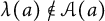 $\lambda (a)\not \in {\cal A}(a)$
implies
 $T_m(\lambda (a))=\infty $
. Assume that there exists
 $t_0\in [0,\infty )$
such that
 $I(u_{\lambda (a)}(t_0))<d_\infty $
. Then, Lemma A.1 (together with
 $T_m(\lambda )=\infty $
) assures that
 $u(t)\to 0$
in
 $H^1({\mathbb {R}^N})$
as
 $t\to \infty $
, namely,
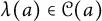 $\lambda (a)\in {\cal C}(a)$
and this is against the conclusion of Lemma A.2.
Sketch of proof of Lemma 1.1
First, we note that the energy decreasing property (1.3) and Lemma A.3 yield
 $$ \begin{align} d_\infty\leq I(u_{\lambda (a)}u(t))\leq I(\lambda (a)a)\leq \max_{\mu>0}I(\mu a)=I(\mu(a) a), \end{align} $$
where
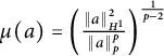 $\mu (a)=\left (\frac {\|a\|_{H^1}^2}{\|a\|_p^p} \right )^{\frac {1}{p-2}}$
. Since
 $$ \begin{align*}\mu(a)\to \mu(w)= \left(\frac{\|w\|_{H^1}^2}{\|w\|_p^p} \right)^{\frac{1}{p-2}}=1 \end{align*} $$
as
 $a\to w$
in
 $H^1({\mathbb {R}^N})$
, we have
 $$ \begin{align} I(\mu(a) a)=\frac{\mu(a)^2}{2}\|a\|_{H^1}^2- \frac{\mu(a)^p}{p}\|a\|_p^p \to I(w)=d_\infty \end{align} $$
as
 $a\to w$
in
 $H^1({\mathbb {R}^N})$
. Relations (A.1) and (A.2) show that there exists
 $a\in H^1({\mathbb {R}^N})$
with
 $a\not \in E$
(see (1.11) for the definition of E) such that
 $$ \begin{align} I(\lambda (a)a)\in [d_\infty,2d_\infty). \end{align} $$
Without loss of generality, we can assume that
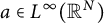 $a\in L^\infty ({\mathbb {R}^N})$
and
 $\mathop {\mathrm {supp}} a$
is noncompact. Now we show that
 $$ \begin{align} I(\lambda (a)a)>d_\infty \end{align} $$
(actually, we can show
 $I(u_{\lambda (a)}(t))>d_\infty $
for
 $t>0$
by following the same argument). Indeed, if not, then (A.1) assures
 $d_\infty \leq I(u_{\lambda (a)}u(t))\leq I(\lambda (a)a)=d_\infty $
, which yields
 $u_{\lambda (a)}u(t)$
is a nontrivial nonnegative stationary solution of (P). This fact and the uniqueness of the nonnegative stationary solution of (P) modulo spatial translation implies
 $a\in E$
, a contradiction.
Now, let
 $u_0:=\lambda (a)a$
. Then, (A.1), (A.3), and (A.4) assure that
 $u_0\in H^1({\mathbb {R}^N})\cap L^\infty ({\mathbb {R}^N})$
is a nonnegative function with noncompact support satisfying
 $$ \begin{align} I(u_0)\in (d_\infty,2d_\infty),\quad I(u(t))\in [d_\infty,2d_\infty),\ t\geq 0, \end{align} $$
where u denotes a solution of (P) with
 $u_0$
above, thus u is a nontrivial global-in-time solution of (P). Then for any
 $(t_n)$
with
 $t_n\to \infty $
as
 $n\to \infty $
, Proposition 2.1 leads the existence of
 $M\in {\mathbb {N}}$
such that
 $$ \begin{align*} I(u(t_n)) &=\frac{1}{2}\|u(t_n)\|_{H^1}^2- \frac{1}{p}\|u(t_n)\|_p^p = \frac{1}{2}\sum_{j=1}^M\|w\|_{H^1}^2 - \frac{1}{p}\sum_{j=1}^M\|w\|_p^p+o(1)\notag\\ &=Md_\infty+o(1) \end{align*} $$
as
 $n\to \infty $
passing to a subsequence if necessary. This relation and the second relation in (A.5) ensure
 $M=1$
, hence
 $$ \begin{align} I(u(t))\downarrow d=d_\infty\text{ as }t\to\infty. \end{align} $$
A.2 A sketch of proof of (1.3)
The following argument is essentially due to Levine [Reference Levine18] (see also [Reference Ibrahim, Jrad, Majdoub and Saanouni10, Proposition 4.7]). We will show
 $$ \begin{align} T_m<\infty \end{align} $$
under the assumption of the existence of
 $t_0\in [0,T_m)$
satisfying
 $$ \begin{align} I(u(t_0))<0. \end{align} $$
It is easy to see that this immediately yields (1.3).
Under the assumption (A.8), suppose that (A.7) does not hold, namely, there holds
 $$ \begin{align*} T_m=\infty. \end{align*} $$
Note that by multiplying u to (P) and integrating over
 ${\mathbb {R}^N}$
, we have
 $$ \begin{align*} \frac{d}{dt}\frac{1}{2}\|u(t)\|_2^2=-\|u(t)\|_{H^1}^2+\|u(t)\|_p^p. \end{align*} $$
For
 $$ \begin{align*} y(t)=\frac{1}{2}\int_{t_0}^tds\|u(s)\|_2^2, \end{align*} $$
the relation above with (A.8) and the energy equality (1.2) yields
 $$ \begin{align} y"(t) = -\|u(t)\|_{H^1}^2+\|u(t)\|_p^p \geq p(-I(u(t))) \geq p(-I(u(t_0)))>0, \end{align} $$
hence
 $$ \begin{align} y(t),\,y'(t)\to\infty\text{ as }t\to\infty. \end{align} $$
Also (A.8) and the energy equality (1.2) lead
 $$ \begin{align*} -I(u(t))=\int_{t_0}^{t}ds\|\partial_s u(s)\|_2^2-I(u(t_0))\geq \int_{t_0}^{t}ds\|\partial_s u(s)\|_2^2, \end{align*} $$
which together with (A.9) yields
 $$ \begin{align*} y"(t)\geq p\int_{t_0}^{t}ds\|\partial_s u(s)\|_2^2. \end{align*} $$
Then, we have
 $$ \begin{align*} \frac{p}{2}[y'(t)-y'(t_0)]^2 &= \frac{p}{2}\left(\int_{t_0}^tds\frac{1}{2}\frac{d}{ds}\|u(s)\|_2^2 \right)^2\\&\leq \frac{p}{2}\left(\int_{t_0}^tds\|\partial_su(s)\|_2\|u(s)\|_2\right)^2 \nonumber\\&\leq \frac{p}{2}\int_{t_0}^tds \|\partial_su(s)\|_2^2\int_{t_0}^tds\|u(s)\|_2^2 \leq y"(t)y(t). \end{align*} $$
This relation together with (A.10) assures that, for
 $\beta>0$
with
 $1+\beta <\frac {p}{2}$
, there exists
 $\tau _\beta \geq t_0$
such that
 $$ \begin{align*} (1+\beta)[y'(t)]^2< y"(t)y(t),\quad t\geq\tau_\beta. \end{align*} $$
Note that, this relation yields, for
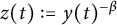 $z(t):=y(t)^{-\beta }$
,
 $$ \begin{align*} z"(t) = \beta y(t)^{-\beta-2}\left[(1+\beta)[y'(t)]^2- y"(t)y(t)\right] <0,\quad t\geq\tau_\beta, \end{align*} $$
which contradicts
 $$ \begin{align*} z(t)=y(t)^{-\beta}\to 0\text{ as }t\to\infty \end{align*} $$
A.3 A sketch of proof of Lemma 2.1
Assume
 $$ \begin{align} p\in \left[2+\frac{2}{N},2^*\right). \end{align} $$
Suppose that (2.3) does not hold. Then there exist
 $(t_n)$
with
 $t_n\to \infty $
as
 $n\to \infty $
and
 $(x_n)\subset {\mathbb {R}^N}$
such that
 $$ \begin{align} \sup_{t\leq t_n}\|u(t)\|_\infty=\|u(t_n)\|_\infty=|u(x_n,t_n)|\to\infty\text{ as }n\to\infty. \end{align} $$
We introduce a sequence
 $(v_n)$
of rescaled u by
 $$ \begin{align*} v_n(y,s):=\lambda_n^{\frac{2}{p-2}}u(x,t),\quad y\in B(0,1),\quad s\in [-1,0], \end{align*} $$
where
 $$ \begin{align*} x=x_n+\lambda_ny,\quad t=t_n+\lambda_n^2s,\quad \lambda_n^{\frac{2}{p-2}}=|u(x_n,t_n)|^{-1}. \end{align*} $$
Note that
 $(v_n)$
satisfy
 $$ \begin{align} &|v_n(y,s)|\leq 1\text{ for }y\in B(0,1),\ s\in [-1,0] , \end{align} $$
 $$ \begin{align} &|v_n(0,0)|=1. \end{align} $$
Also the relation (A.12) yields
 $$ \begin{align} \lambda_n\to 0\text{ as }n\to\infty. \end{align} $$
By the transformation above, we have the following equation for
 $(v_n)$
from (P):
 $$ \begin{align*} \text{(Q)}\quad \partial_sv_n=\Delta v_n-\lambda_n^2v_n+v_n|v_n|^{p-2},\quad y\in B(0,1),\ s\in [-1,0]. \end{align*} $$
Since we have (A.15) and the uniform bound (A.13), the standard parabolic regularity indicates the existence of
 $v\in C(B(0,1)\times [-1,0])$
satisfying
 $$ \begin{align} v_n\to v\text{ in }C(B(0,1)\times [-1,0]), \end{align} $$
see, e.g., [Reference Giga9, Lemma]. Moreover, (A.14) yields
 $$ \begin{align*} 1=|v_n(0,0)|\to |v(0,0)|,\end{align*} $$
hence there exists
 $\rho>0$
and
 $\sigma>0$
such that
 $$ \begin{align} \frac{1}{2}\leq |v(y,s)|,\quad (y,s)\in B(0,\rho)\times [-\sigma,0]. \end{align} $$
Now, let
 $$ \begin{align*} U_n(\cdot):=u(\cdot-x_n,t_n). \end{align*} $$
Then,
 $(U_n)\subset H^1(B(0,1))$
is a bounded sequence in view of the
 $H^1$
-global bounds (1.6). Also note that the assumption (A.11) on p yields
 $$ \begin{align*} p_0:=\frac{N}{2}(p-2)\in [1,2^*), \end{align*} $$
thus the embedding
 $H^1(B(0,\rho ))\hookrightarrow L^{p_0}(B(0,\rho ))$
is compact. These facts show the existence of
 $U\in H^1(B(0,1))$
satisfying
 $$ \begin{align*} U_n\to U\text{ in }L^{p_0}(B(0,1))\text{ as }n\to\infty \end{align*} $$
along subsequence. Thus, for
 $\varepsilon \in (0,1)$
,
 $$ \begin{align} \int_{B(0,\varepsilon)}|U_n|^{p_0}\to \int_{B(0,\varepsilon)}|U|^{p_0}\text{ as }n\to\infty. \end{align} $$
Note that
 $$ \begin{align*} \int_{B(0,\rho)}|v_n|^{p_0} =\int_{B(x_n,\lambda_n\rho)}|u(\cdot,t_n)|^{p_0} \leq \int_{B(0,\varepsilon)}|U_n|^{p_0}\text{ for large }n, \end{align*} $$
since
 $\lambda _n\to 0$
. This relation with (A.16) and (A.18) yields
 $$ \begin{align*} \int_{B(0,\rho)}|v|^{p_0} \leq \int_{B(0,\varepsilon)}|U|^{p_0}, \end{align*} $$
which together with (A.17) implies
 $$ \begin{align*} \frac{1}{2}|B(0,\rho)| \leq \int_{B(0,\varepsilon)}|U|^{p_0},\quad\varepsilon\in (0,1). \end{align*} $$
By letting
 $\varepsilon \to 0$
, we have a contradiction.
Acknowledgment
The authors would like to thank Dr. Li Haoyu for their useful discussions and comments on the first version of this article.



