



1 Introduction
The question whether the hierarchy of Bounded Arithmetic theories is strict or not, is an important open problem due to its connections to corresponding questions about levels of the Polynomial Time Hierarchy [Reference Buss2]. One obvious way to address this problem is to make use of Gödel’s 2nd Incompleteness Theorem, using statements expressing consistency for Bounded Arithmetic theories. Early lines of research aimed to restrict the formulation of consistency suitably to achieve this aim [Reference Buss2, Reference Pudlák8], with limited success.
One particular programme is to consider consistency statements based on equational theories. Buss and Ignjatović [Reference Buss and Ignjatovic4] have shown that the consistency of an induction free version of Cook’s equational theory PV [Reference Cook5] is not provable in
 $\mathrm {S}^{1}_2 $
, where
 $\mathrm {S}^{1}_2 $
is the Bounded Arithmetic theory related to polynomial time reasoning. Their version of induction free PV is formulated in a system that allows, in addition to equations, also inequalities between terms, and Boolean formulas. Furthermore, a number of properties have been stated as axioms.
On the other hand, in a pure equational setting, where lines in derivations are equations between terms, where axioms are restricted to recursive definitions of function symbols, and where induction is not allowed, consistency becomes provable in Bounded Arithmetic: The first author has shown in [Reference Beckmann1] that the consistency of pure equational theories, in which substitution is not allowed, is provable in
 $\mathrm {S}^{1}_2 -$
in particular this result applies to Cook’s PV [Reference Cook5] without substitution and induction. The second author of this paper has improved on this result in [Reference Yamagata10] by showing that the consistency of PV without induction but with substitution is provable in
 $\mathrm {S}^{2}_2 $
, the second level of the hierarchy of Bounded Arithmetic theories.
In this paper, we extend both our previous results [Reference Beckmann1, Reference Yamagata10]. With
 $\textbf {PETS} (\mathrm {Ax} )$
we denote the pure equational theory with substitution but without induction, based on a ‘set of nice axioms
 $\mathrm {Ax} $
’—we will make the notion of ‘nice axioms’ precise in Definition 6. Cook’s original PV [Reference Cook5] without induction but with substitution is one example of a pure equational theory in this sense. The main aim of this paper is to show that the consistency of
 $\textbf {PETS} (\mathrm {Ax} )$
is provable in
 $\mathrm {S}^{1}_2 $
, thus improving on both [Reference Beckmann1, Reference Yamagata10]. To this end we employ a novel method of defining pre-models in Bounded Arithmetic based on approximate values, which may be of independent interest. Our approach resembles elements from domain theory, however we leave a full treatment of domain theory in Bounded Arithmetic to future research.
In the next section, we briefly introduce Bounded Arithmetic and fix some notions used throughout the paper. In Section 3 we define pure equational theories
 $\textbf {PETS} (\mathrm {Ax} )$
, which will be more general than PV without induction in that arbitrary recursive functions may be considered. This is followed in Section 4 by an introduction of approximate values and semantics based on approximation, leading to feasible evaluations of terms based on such approximation semantics. Section 5 then defines pre-models for equational theories based on approximation semantics, including a suitably restricted version which can be expressed as a bounded formula and used in induction arguments inside Bounded Arithmetic. A key notion will be a way of updating such pre-models with further information about approximate values of functions, in a way that preserves the notion of being a pre-model, provably in
 $\mathrm {S}^{1}_2 $
. In Section 6 we prove our first main theorem showing a form of soundness for
 $\textbf {PETS} (\mathrm {Ax} )$
based on approximation semantics in
 $\mathrm {S}^{2}_2$
– an immediate consequence will be that
 $\mathrm {S}^{2}_2 $
proves the consistency of
 $\textbf {PETS} (\mathrm {Ax} )$
. The final sections improve on this approach to obtain the main result in
 $\mathrm {S}^{1}_2 $
: In Section 7 we introduce instructions which are extracted from derivations in
 $\textbf {PETS} (\mathrm {Ax} )$
and store key steps in the construction of updates of models. In this way we obtain an explicit way of describing pre-model constructions related to
 $\textbf {PETS} (\mathrm {Ax} )$
derivations, which allows us to reduce the bounded quantifier complexity of induction assertions in the proof of our second main theorem in Section 8 to show an improved soundness property for
 $\textbf {PETS} (\mathrm {Ax} )$
provable in
 $\mathrm {S}^{1}_2 $
.
2 Bounded Arithmetic
2.1 Language of Bounded Arithmetic
We give a brief introduction to Bounded Arithmetic to support the developments in this paper. For more in depth discussions and results we refer the interested reader to the literature [Reference Buss2, Reference Krajíček6]. Theories of Bounded Arithmetic are first order theories of arithmetic similar to Peano Arithmetic, their domain of discourse is the set of non-negative integers. For the purpose of this paper we can assume that the language of Bounded Arithmetic contains a symbol for each polynomial time computable function, including
 $0$
,
 $1$
,
 $+$
,
 $\cdot $
,
 $|.|$
,
 $\mathbin {\#}$
, representing zero, one, addition, multiplication, the binary length function
 $|x|$
that computes the number of bits in a binary representation of x and can be defined by
 $|x|=\lceil \log _2(x+1)\rceil $
, and smash
 $\mathbin {\#}$
computing
 $x\mathbin {\#} y=2^{|x|\cdot |y|}$
.
2.2 Theories of Bounded Arithmetic
Theories of Bounded Arithmetic contain suitable defining axioms for their function symbols. The main differences are various forms of induction for various classes of bounded formulas, which we will define next.
Bounded quantifiers are defined as follows:
 $$ \begin{align*} (\forall x\le t)A &\quad\text{abbreviates}\quad (\forall x) (x\le t\rightarrow A) \\ (\exists x\le t)A &\quad\text{abbreviates}\quad (\exists x) (x\le t\wedge A). \end{align*} $$
If the bounding term t of a bounded quantifier is of the form
 $|t'|$
, then the quantifier is called sharply bounded.
Classes of bounded formulas
 $\Sigma ^{\mathrm {b}}_{i} $
and
 $\Pi ^{\mathrm {b}}_{i} $
are defined in [Reference Buss2] by essentially counting alternations between existential and universal bounded quantifiers. Predicates defined by
 $\Sigma ^{\mathrm {b}}_{i} $
and
 $\Pi ^{\mathrm {b}}_{i} $
formulas define computational problems in corresponding classes of the Polynomial Time Hierarchy of decision problems
 $\Sigma ^{\mathrm {p}}_{i} $
and
 $\Pi ^{\mathrm {p}}_{i} $
, respectively. For example, those defined by
 $\Sigma ^{\mathrm {b}}_{1} $
correspond exactly to
 $\Sigma ^{\mathrm {p}}_{1} $
, i.e., NP.
In particular, the
 $\Sigma ^{\mathrm {b}}_{i} $
and
 $\Pi ^{\mathrm {b}}_{i} $
classes include the following formulas:
-
•
 $\Sigma ^{\mathrm {b}}_{0} =\Pi ^{\mathrm {b}}_{0} $
is the class of formulas built from atomic formulas and closed under Boolean connectives and sharply bounded quantification.
-
•
$\Sigma ^{\mathrm {b}}_{i+1} $
includes all formulas of the form
$(\exists x\le t)A$
with
$A\in \Pi ^{\mathrm {b}}_{i} $
. -
•
$\Pi ^{\mathrm {b}}_{i+1} $
includes all formulas of the form
$(\forall x\le t)A$
with
$A\in \Sigma ^{\mathrm {b}}_{i} $
.


The theories
 $\mathrm {S}^{i}_2 $
,
 $i\ge 0$
, of Bounded Arithmetic have been defined in [Reference Buss2], establishing a close relationship between fragments of Bounded Arithmetic and levels of the Polynomial Time Hierarchy of functions. More precisely, the
 $\Sigma ^{\mathrm {b}}_{i+1} $
-definable functions of
 $\mathrm {S}^{i+1}_2 $
, that is the functions whose graph can be described by a
 $\Sigma ^{\mathrm {b}}_{i+1} $
formula, and whose totality is provable in
 $\mathrm {S}^{i+1}_2 $
, form exactly the
 $i{+}1$
-st level of the Polynomial Time Hierarchy of functions,
 $\mathrm {FP}^{\Sigma ^{\mathrm {p}}_{i} }$
.
Instead of defining the theory
 $\mathrm {S}^{i}_2 $
, we state some characteristic properties about induction provable in them. Let
 $\Sigma ^{\mathrm {b}}_{i} \text {-IND} $
be the schema of induction for
 $\Sigma ^{\mathrm {b}}_{i} $
-properties, consisting of formulas of the form
 $$\begin{align*}A(0) \wedge (\forall x)(A(x)\rightarrow A(x+1)) \rightarrow (\forall x)A(x) \end{align*}$$
for
 $A\in \Sigma ^{\mathrm {b}}_{i} $
. The schema of logarithmic induction
 $\Sigma ^{\mathrm {b}}_{i} \text {-LIND} $
is then obtained by restricting the conclusion of induction to logarithmic values, that is
 $$\begin{align*}A(0) \wedge (\forall x)(A(x)\rightarrow A(x+1)) \rightarrow (\forall x)A(|x|) \end{align*}$$
for
 $A\in \Sigma ^{\mathrm {b}}_{i} $
.
We have the following:
Theorem 1 [Reference Buss2].
The instances of
 $\Sigma ^{\mathrm {b}}_{i} \text {-LIND} $
and
 $\Pi ^{\mathrm {b}}_{i} \text {-LIND} $
are provable in
 $\mathrm {S}^{i}_2 $
.
We already mentioned the intricate relationship between Bounded Arithmetic theories and the Polynomial Time Hierarchy in terms of definable functions. Furthermore, it is known that a collapse of the hierarchy of Bounded Arithmetic theories is equivalent to the provability in Bounded Arithmetic of a collapse of the Polynomial Time Hierarchy [Reference Samuel3, Reference Krajiček, Pudlák and Takeuti7, Reference Zambella11]. With
 $\mathrm {T}^{i}_2 $
denoting the theory defined by
 $\Sigma ^{\mathrm {b}}_{i} \text {-IND} $
, we have that
 $\mathrm {T}^{i}_2 =\mathrm {S}^{i+1}_2 $
is equivalent to
 $\Sigma ^{\mathrm {p}}_{i+1} \subseteq \Pi ^{\mathrm {p}}_{i+1} /\mathit {poly}$
provable in
 $\mathrm {T}^{i}_2 $
.
The Bounded Arithmetic theory
 $\mathrm {S}^{1}_2 $
is able to formalize meta-mathematics and essential constructions to prove Gödel’s Incompleteness theorems [Reference Buss2]. A basis for such formalization is a feasible encoding of sequences of numbers. For this paper we assume that a suitable encoding of sequences and operations on them can be formalized in
 $\mathrm {S}^{1}_2 $
as done in [Reference Buss2]. We assume the following notation:
-
• With
$\langle {x_1, \dots , x_k} \rangle $
we denote the encoding of sequence
$x_1, \dots , x_k$
. We will use
$\sigma $
,
$\tau $
etc to range over sequence encodings. -
• With ‘
$\mathbin {\,{:}{:}\,}$
’ we denote concatenation of sequences:
$$\begin{align*}\langle {x_1, \dots, x_k} \rangle \mathbin{\,{:}{:}\,} \langle {x_{k+1}, \dots, x_{k+\ell}} \rangle \quad=\quad \langle {x_{1}, \dots, x_k, x_{k+1}, \dots, x_{k+\ell}} \rangle \end{align*}$$
-
• With ‘
$\mathbin {\,{:}\,}$
’ we denote the function that adds an element to the left or right of a sequence:
$$ \begin{align*} x \mathbin{\,{:}\,} \sigma &\quad=\quad \langle {x} \rangle \mathbin{\,{:}{:}\,} \sigma \\ \sigma \mathbin{\,{:}\,} x &\quad=\quad \sigma \mathbin{\,{:}{:}\,} \langle {x} \rangle \end{align*} $$


The predicate ‘being a sequence encoding’, as well as the operations ‘
 $\mathbin {\,{:}\,}$
’ and ‘
 $\mathbin {\,{:}{:}\,}$
’, can be defined in
 $\mathrm {S}^{1}_2 $
with their usual properties proven.
In the following, in order to argue that transformations and constructions involving syntax (like terms, proofs, etc) can be conducted in Bounded Arithmetic, we will focus on the length of objects, instead of their size as given by e.g., number of bits in a suitable Gödelization. For an object o we will define its length
 $\operatorname {\mathrm {\mathbf {l}}}(o)$
to be the number of symbols occurring in o. As all our constructions will happen in the context of a given derivation
 $\mathcal {D}$
, we obtain that the size of the Gödelization of object o can then be bounded by
 $\operatorname {\mathrm {\mathbf {l}}}(o)$
times the size of the Gödelization of
 $\mathcal {D}$
.
Furthermore, the constructions for defining o in the context of
 $\mathcal {D}$
will always be explicit and simple enough to be formalizable in
 $\mathrm {S}^{1}_2 $
, similar to constructions in [Reference Buss2] dealing with meta-mathematical notions. In those cases where more involved induction is needed (as in Theorems 42 and 53) these will be analyzed carefully.
2.3 Notations
In the remaining part of this section we will fix some notation used throughout this paper. We use
 $\equiv $
for equality of syntax.
-
• With
$\# S$
we denote the cardinality of a set S. -
• For a function f,
$\operatorname {{\mathrm {dom}}}(f)$
denotes its domain,
$\operatorname {{\mathrm {rng}}}(f)$
its range. -
• For a set S, tuples in
$S^n$
are denoted with
$(s_1,\dots ,s_n)$
. -
• We use the notation
$\overline {{s}}$
for a tuple
$(s_1, \ldots , s_n)$
as well as a sequence
$s_1, \ldots , s_n$
of objects. -
•
$\max (X)$
computes the maximum (according to a given order) of the elements in X.
$\max $
is applied to a tuple by computing the maximal component in it.


Remark. Technically, there is a difference between a tuple of the form
 $(s_1,\dots ,s_n)$
, which is an element of
 $S^n$
, and the sequence
 $s_1,\dots ,s_n$
, which is a formal list used e.g., as the arguments to an n-ary function. We will identify both and write
 $\overline {{s}}\in S^n$
and
 $f(\overline {{s}})$
in the same context, as long as it does not lead to confusion, in which case we will choose a more precise differentiation.
3 Equational theories
3.1 Domain of discourse
The intended domain of discourse
 $\mathbb {B}$
are finite binary strings representing numbers.
 $\mathbb {B}$
can be defined inductively as follows:
 $$ \begin{align*} v ::= \epsilon \mid v0 \mid v1. \end{align*} $$
We will also use terms denoting binary strings, which are formed from constant
 $\epsilon $
using unary function symbols
 $\operatorname {{\mathrm {s}}}_0$
and
 $\operatorname {{\mathrm {s}}}_1$
to add a single digit to the right of a string. We also use
 $t0$
to denote
 $\operatorname {{\mathrm {s}}}_0(t)$
, and
 $t1$
for
 $\operatorname {{\mathrm {s}}}_1(t)$
for terms t, following Cook [Reference Cook5]. We will drop
 $\epsilon $
when writing explicit binary strings, e.g., writing
 $1101$
instead of
 $\epsilon 1101$
, or
 $\operatorname {{\mathrm {s}}}_1(\operatorname {{\mathrm {s}}}_0(\operatorname {{\mathrm {s}}}_1(\operatorname {{\mathrm {s}}}_1(\epsilon ))))$
.
Remark. There is a choice in notation in that bits can go to the right or left of v. Going to the left would follow domain theory convention where the focus are infinite binary strings. We decided to put them to the right, following Bounded Arithmetic convention as initiated by Cook [Reference Cook5], because the focus in this paper are finite binary strings representing numbers.
Remark. Our results are not restricted to finite binary strings, but can be applied to general free algebras as domains of discourse as done in [Reference Beckmann1]. However, for sake of simplicity we will only consider binary strings in this paper.
3.2 Terms
We fix the language we use for equational theories.
Definition 2 (Language for Equational Theories).
We have the following basic ingredients:
-
• A countable set
$\mathcal {X}$
of variables; we use
$x, y, x_1, x_2, \ldots $
to denote variables. -
• A countable set
$\mathcal {F}$
of function symbols; we use
$f, g, h,f_1, f_2, \ldots $
to denote function symbols. Each function
$f\in \mathcal {F}$
comes with a non-negative integer
$\operatorname {{\mathrm {ar}}}(f)$
called its arity. We assume that
$\epsilon $
,
$\operatorname {{\mathrm {s}}}_0$
and
$\operatorname {{\mathrm {s}}}_1$
are included in
$\mathcal {F}$
;
$\epsilon $
,
$\operatorname {{\mathrm {s}}}_0$
and
$\operatorname {{\mathrm {s}}}_1$
form the set
$\mathcal {B}$
of basic function symbols.


Remark. A function with arity
 $0$
is called a constant. For example,
 $\epsilon $
is a constant.
Definition 3 (Terms).
Let
 $X\subseteq \mathcal {X}$
and
 $F\subseteq \mathcal {F}$
. The set
 $\mathcal {T}(X,F)$
of terms over F and X, or simply terms, is defined inductively as follows:
-
• All variables in X are terms.
-
• If
$f\in F$
has arity n and
$t_1, \ldots , t_n$
are terms, then
$f(t_1, \ldots , t_n)$
is a term.


We will use
 $s,t,u$
to denote terms.
The length
 $\operatorname {\mathrm {\mathbf {l}}}(t)$
of term t is defined in the following way: The length of a variable is
 $1$
, and, recursively,
 $$\begin{align*}\operatorname{\mathrm{\mathbf{l}}}(f(t_1, \dots, t_n)) = \operatorname{\mathrm{\mathbf{l}}}(t_1)+\dots+\operatorname{\mathrm{\mathbf{l}}}(t_n)+1 \enspace. \end{align*}$$
With
 $\operatorname {{\mathrm {Var}}}(t)$
we denote the set of variables that are occurring in a term t. For S a set of terms,
 $\operatorname {{\mathrm {Var}}}(S)$
denotes the union of
 $\operatorname {{\mathrm {Var}}}(t)$
for
 $t \in S$
.
Definition 4 (Substitution).
Let
 $t,u$
be terms and x be a variable. The substitution of u for x in t, denoted
 $t[u/x]$
, is obtained by replacing any occurrence of x in t by u.
We extend substitution to sequences of variables and terms of the same length by successively substituting terms:
 $t[\overline {{u}}/\overline {{x}}]$
stands for
 $t[u_1/x_1][u_2/x_2]\dots [u_n/x_n]$
.
Definition 5 (Instance and injective renaming).
A substitution instance, or instance, of an equation
 $s=t$
is any
 $s[\overline {{u}}/\overline {{x}}] = t[\overline {{u}}/\overline {{x}}]$
for terms
 $\overline {{u}}$
.
An instance
 $s[\overline {{u}}/\overline {{x}}]=t[\overline {{u}}/\overline {{x}}]$
is called an injective renaming of
 $s=t$
, iff
 $\{\overline {{x}}\}=\operatorname {{\mathrm {Var}}}(s) \cup \operatorname {{\mathrm {Var}}}(t)$
, and
 $\overline {{u}}$
is a list of pairwise distinct, fresh variables.
3.3 Nice axiom systems
We will consider axioms consisting of equations that satisfy particular conditions, which have been called nice in [Reference Beckmann1].
Definition 6 (Nice axioms, [Reference Beckmann1]).
Let
 $\mathrm {Ax} $
be a set of equations over
 $\mathcal {F}$
.
 $\mathrm {Ax} $
is called a set of nice axioms for
 $\mathcal {F}$
, if the following is satisfied: Each equation in
 $\mathrm {Ax} $
must be of one of the following forms, for some
 $f\in \mathcal {F}\setminus \mathcal {B}$
, some
 $t, t_\epsilon \in \mathcal {T}(\mathcal {F},\{\overline {{y}}\})$
, and
 $t_0, t_1\in \mathcal {T}(\mathcal {F},\{x,\overline {{y}}\})$
:
 $$ \begin{align*} f(\overline{{y}}) &= t \\ f(\epsilon, \overline{{y}}) &= t_\epsilon \\ f(x0, \overline{{y}}) &= t_0 \\ f(x1, \overline{{y}}) &= t_1. \end{align*} $$
Furthermore, the left-hand side of an equation is occurring at most once among equations in
 $\mathrm {Ax} $
, also modulo injective renamings.
Henceforth,
 $\mathrm {Ax} $
is a set of nice axioms.
Remark. The definition implies that for any
 $t=u$
in
 $\mathrm {Ax} $
we have
 $\operatorname {{\mathrm {Var}}}(u)\subseteq \operatorname {{\mathrm {Var}}}(t)$
.
Remark. Consider a term
 $f(\overline {{s}})$
with
 $f\in \mathcal {F}\setminus \mathcal {B}$
. The property of
 $\mathrm {Ax} $
being nice implies that there is at most one axiom
 $t=u$
in
 $\mathrm {Ax} $
such that
 $f(\overline {{s}})$
can be written as a substitution instance of t.
Remark. For the reader familiar with term-rewriting we remark that the term rewriting system induced by nice axioms is orthogonal, which follows from the previous two remarks.
Remark. The definition of a nice axiom system in [Reference Beckmann1] also contains a completeness condition, requiring that each function symbol in
 $\mathcal {F}\setminus \mathcal {B}$
is defined by an equation, and that the case distinction in the latter part is complete. We omit this form of completeness, as it is not needed for our developments.
The left-hand side of an equation in
 $\mathrm {Ax} $
is of a very special form: an argument to the outermost function symbol can either be a variable,
 $\epsilon $
,
 $x0$
, or
 $x1$
for some variable x. We capture these forms in the following definition.
Definition 7 (Generalized variable).
A generalized variable is a term which either is a variable, or
 $\epsilon $
, or of the form
 $x0$
or
 $x1$
for some variable x.
Remark. Consider an axiom
 $t=u$
in
 $\mathrm {Ax} $
. It follows that t must be of the form
 $f(\overline {{s}})$
, that each
 $s_i$
is a generalized variable, hence each
 $s_i$
contains at most one variable. Furthermore, the same variable cannot occur simultaneously in
 $s_i$
and
 $s_j$
for
 $i\neq j$
.
Definition 8 (Rules for equational reasoning).
Let
 $s,t,u$
represent terms, and x a variable. The following are the rules that can be used to derive equations:
-
Axiom:
$\vdash t=u$
, where
$t=u$
is an injective renaming of an equation in
$\mathrm {Ax} $
. -
Reflexivity:
$\vdash t=t$
-
Symmetry:
$t=u \vdash u=t$
-
Transitivity:
$t=s,s=u \vdash t=u$
-
Compatibility:
$t=u \vdash s[t/x] = s[u/x]$
-
Substitution:
$t=u \vdash t[s/x] = u[s/x]$
.


In the case of Substitution as stated above, we say that the application of Substitution binds the variable x.
Remark. We also make use of a display style for presenting rules, like

for Reflexivity Rule, or

for Transitivity Rule. As indicated, we may abbreviate the rule that is used by its first two letters.
Definition 9 (Derivations).
A derivation is a finite tree whose nodes are labelled with rules for equational reasoning, such that for each node, the premises of the rule at that node coincide with the conclusions of rules at corresponding child nodes.
Derivations can also be defined inductively from rules for equational reasoning: Any axiom or Reflexivity Rule is a derivation ending in the equation given by that rule. If R is a unary rule (like Symmetry, Compatibility or Substitution) with premise
 $e'$
and conclusion e, and
 $\mathcal {D}'$
a derivation ending in
 $e'$
, then

is a derivation ending in e. The only binary rule we are considering is the Transitivity Rule. If
 $\mathcal {D}_1$
a derivation ending in
 $t=s$
, and
 $\mathcal {D}_2$
a derivation ending in
 $s=u$
, then

is a derivation ending in
 $t=u$
.
We tacitly assume that labels of rules carry information to uniquely identify them. For example, in the case of Compatibility and Substitution in Definition 8, the label would contain x and s.
Building on Definition 3, the length
 $\operatorname {\mathrm {\mathbf {l}}}(t=u)$
of an equation
 $t=u$
is set to
 $\operatorname {\mathrm {\mathbf {l}}}(t)+\operatorname {\mathrm {\mathbf {l}}}(u)+1$
. The length
 $\operatorname {\mathrm {\mathbf {l}}}(l)$
of a label l of a rule R is set to either
 $\operatorname {\mathrm {\mathbf {l}}}(s) + \operatorname {\mathrm {\mathbf {l}}}(x) + 1$
if R is Compatibility or Substitution involving x and s, or
 $1$
otherwise. The length
 $\operatorname {\mathrm {\mathbf {l}}}(\mathcal {D})$
of a derivation
 $\mathcal {D}$
is defined as the sum of the lengths of the equations and labels of rules occurring in it.
With
 $\operatorname {{\mathrm {Var}}}(\mathcal {D})$
we denote the set of variables occurring in
 $\mathcal {D}$
.
 $\operatorname {{\mathrm {BVar}}}(\mathcal {D})$
is the set of variables occurring in
 $\mathcal {D}$
that are bound by an application of the Substitution Rule.
Definition 10 (Pure equational theories with substitution).
The pure equational theory with substitution
 $\textbf {PETS} (\mathrm {Ax} )$
consists of all equations that can be derived using the Axiom rules for
 $\mathrm {Ax} $
, as well as the Reflexivity, Symmetry, Transitivity, Compatibility, and Substitution Rules.
Definition 11 (Variable Normal Form).
A
 $\textbf {PETS} (\mathrm {Ax} )$
derivation
 $\mathcal {D}$
is in variable normal form if each variable occurring in
 $\mathcal {D}$
is either occurring in the equation in which the derivation ends, or is removed in exactly one application of Substitution (as the variable which is bound by that application of Substitution).
Proposition 12. Assume
 $\mathcal {D}\vdash t=u$
, then there exists
 $\mathcal {D}'$
in variable normal form of same length as
 $\mathcal {D}$
such that
 $\mathcal {D}'\vdash t=u$
.
Proof. We observe that we can replace all occurrences of a fixed variable by a fresh variable throughout a derivation ending in an equation e, obtaining a similar derivation of the equation e, potentially with the former variable being renamed to the latter fresh variable. This transformation works as our derivations are tree-like. The above transformation does not change the length of the derivation.
Remark. While the length does not change when transforming a derivation to variable normal form, its size (in the sense of number of bits in a suitable Gödelization) in general will change due to the need of choosing new indices for fresh variables. As remarked before, the size of the resulting derivation in variable normal form will be bounded by a constant times the product of the length of the new and the size of the original derivation.
Definition 13 (Formal consistency).
With
 $\mathrm {Cons}(\textbf {PETS} (\mathrm {Ax} ))$
we denote the sentence in the language of Bounded Arithmetic which expresses that there is no derivation in
 $\textbf {PETS} (\mathrm {Ax} )$
ending in
 $0=1$
, where
 $0$
, resp.
 $1$
, denotes
 $\epsilon 0$
, resp.
 $\epsilon 1$
.
We close the section with an example theory,
 $\textbf {PETS}_{\mathrm {exp}} $
. The theory defines a form of exponentiation, it will reoccur at later sections to explain terminology defined there.
Example. Let
 $\mathcal {F}_{\mathrm {exp}}$
be
 $\{\epsilon , \operatorname {{\mathrm {s}}}_0, \operatorname {{\mathrm {s}}}_1,\oplus ,\otimes ,\operatorname {{\mathrm {e}}}\}$
where
 $\oplus ,\otimes ,\operatorname {{\mathrm {e}}}$
are binary function symbols.
Let
 $\mathrm {Ax} _{\mathrm {exp}}$
be the nice set of axioms given by
 $$ \begin{align*} x \oplus \epsilon &= x & x \otimes \epsilon &= \epsilon & \operatorname{{\mathrm{e}}}(x, \epsilon) &= 1 \\ x \oplus yi &= (x\oplus y)i & x \otimes yi &= (x\otimes y) \oplus x & \operatorname{{\mathrm{e}}}(x, yi) &= e(x,y) \otimes x \end{align*} $$
for
 $i\in \{0,1\}$
.
For
 $a,b$
terms, consider the following
 $\textbf {PETS}_{\mathrm {exp}} $
derivation of
 $\operatorname {{\mathrm {e}}}(\epsilon ,a\oplus b0)=\epsilon $
. Let
 $\mathcal {D}_1$
denote the derivation

Then let
 $\mathcal {D}_{\mathrm {exp}}$
be

We use a double line to indicate multiple applications of the indicated rule. Here, two applications of substitution are used, one for each variable substituted for.
4 Approximation semantics
A core idea in domain theory is to define finite approximations to functions in a way that is consistent with axioms and equational reasoning. Although we do not develop domain theory fully in this paper, we will make use of some of its notions, and show in particular that those notions can be defined and reasoned with in
 $\mathrm {S}^{1}_2 $
. As constant functions are approximated by themselves, this allows us to conclude that
 $\textbf {PETS} $
will never derive
 $0=1$
, showing that the consistency of
 $\textbf {PETS} $
is provable in bounded arithmetic.
4.1 Approximate values
The notion of approximate values v is defined in [Reference Yamagata10], which adds ‘unknown value’ of a term, as defined in [Reference Beckmann1] and denoted with ‘
 $*$
’, to bit-strings. Infeasible values, although finite, can be considered as infinite bit strings within theories of feasibility like Bounded Arithmetic. From the domain theoretic view, the space of approximate values is a domain formed by infinite strings of bits.
Definition 14 (Approximate values).
The set
 $\mathbb {D}$
of approximate values is defined inductively as follows:
 $$ \begin{align*} v ::= \epsilon \mid v0 \mid v1 \mid *. \end{align*} $$
For the proofs of main theorems we will need a refined approach to measuring length, so that inductive statements in those proofs lead to polynomial bounds. The general principle will be that we think of a typing structure for our objects, so that the i-length of an object of type i is defined in some natural way (like length of a word, or cardinality of a set), while for
 $j<i$
the j-length of a type i object is given as the maximum of the j-lengths of its components. For example, our basic objects will be words in
 $\mathbb {D}$
. They will be of type
 $0$
, and their
 $0$
-length is just their standard length as words. A sequence of words is of type
 $1$
, its
 $1$
-length is its sequence length, i.e., the number of occurrences of words in it, and its
 $0$
-length the maximum of the lengths of words occurring in it. A set of sequences of words is of type
 $2$
, its
 $2$
-length is its cardinality, its
 $1$
-length the maximum of the sequence lengths of its elements, and its
 $0$
-length the maximum of the word lengths of its elements. Etc.
It is then obvious that the length
 $\operatorname {\mathrm {\mathbf {l}}}(o)$
of an object o of type i is bounded by a constant times the product of its j-lengths for
 $j\le i$
.
Definition 15. For an approximate value
 $v\in \mathbb {D}$
, its
 $0$
-length
 ${\mathbf {l}_{0}}(v)$
satisfies
 $$ \begin{gather*} {\mathbf{l}_{0}}(\epsilon) = {\mathbf{l}_{0}}(*) = 1\\ {\mathbf{l}_{0}}(v0) = {\mathbf{l}_{0}}(v1) = {\mathbf{l}_{0}}(v)+1. \end{gather*} $$
For a tuple
 $\overline {{w}} = (w_1, \ldots , w_n) \in \mathbb {D}^n$
, its
 $0$
-length is given as
 $$\begin{align*}{\mathbf{l}_{0}}(\overline{{w}}) = \max\{{\mathbf{l}_{0}}(w_1), \ldots, {\mathbf{l}_{0}}(w_n)\}, \end{align*}$$
and its
 $1$
-length as
 $$\begin{align*}{\mathbf{l}_{1}}(\overline{{w}}) = n. \end{align*}$$
The idea of an approximate value is that bits of higher significance may not be known and are thus replaced by
 $*$
.
Example.
 $1101$
,
 $*01$
,
 $*$
are examples of approximate values,
 $1{*}1$
,
 $**$
are not. Following the above intuition that
 $*$
replaces ‘unknown’ bits of higher significance,
 $*01$
is an approximation to
 $1101$
. We will make this intuition precise in the next subsection.
4.2 Approximation relation
A relation
 $\unlhd $
has been defined in [Reference Beckmann1]. Here we will consider the converse
 $\sqsubseteq $
of
 $\unlhd $
.
Definition 16 (Approximation relation).
The approximation relation
 $\sqsubseteq $
is a binary relation over
 $\mathbb {D}$
, defined inductively as follows:
-
•
$*\sqsubseteq v$
for any
$v \in \mathbb {D}$
. -
•
$\epsilon \sqsubseteq \epsilon $
. -
• if
$v_1 \sqsubseteq v_2$
, then
$v_10 \sqsubseteq v_20$
and
$v_11 \sqsubseteq v_21$
.


We pronounce ‘
 $v\sqsubseteq w$
’ as ‘v approximates w’.
We extend
 $\sqsubseteq $
to tuples:
 $(v_1,\dots ,v_n)\sqsubseteq (w_1,\dots ,w_n)$
iff
 $v_i\sqsubseteq w_i$
for each i.
Example.
 $ *$
approximates any value in
 $\mathbb {D}$
.
 $*01$
approximates
 $1101$
, but does not approximate
 $1010$
.
Proposition 17.
 $\sqsubseteq $
is a partial order on
 $\mathbb {D}^n$
, that is, it is reflexive, anti-symmetric, and transitive.
Definition 18 (Compatibility).
 $u,v\in \mathbb {D}$
are compatible if
 $u \sqsubseteq v$
or
 $v \sqsubseteq u$
.
 $(u_1, \ldots , u_n)$
and
 $(v_1, \ldots , v_n)$
in
 $\mathbb {D}^n$
are compatible if each
 $u_i$
and
 $v_i$
are. We denote
 $\overline {{u}}$
and
 $\overline {{v}}$
being compatible with
 $\overline {{u}} \mathbin {\triangle } \overline {{v}}$
.
The following lemma follows immediately from the definition of compatibility, by induction on the size of the set.
Lemma 19. Any non-empty finite subset S of
 $\mathbb {D}$
of pairwise compatible elements has a maximal element w.r.t.
 $\sqsubseteq $
. We denote the maximal element with
 $\max _\sqsubseteq (S)$
. We also set
 $\max _\sqsubseteq (\emptyset )=*$
.
The following lemma has already been proven in [Reference Beckmann1].
Lemma 20. If
 $\overline {{u}},\overline {{v}},\overline {{w}} \in \mathbb {D}^n$
and
 $\overline {{u}},\overline {{v}} \sqsubseteq \overline {{w}}$
, then
 $\overline {{u}} \mathbin {\triangle } \overline {{v}}$
.
We introduce a couple of notions from the treatment of domain theory as introduced by Vickers [Reference Vickers9].
Definition 21 (Generator, [Reference Vickers9]).
A generator for
 $\mathbb {D}^n \to \mathbb {D}$
is a tuple
 $(\overline {{u}},v)$
, denoted
 $\overline {{u}} \mapsto v$
, with
 $\overline {{u}} \in \mathbb {D}^n$
and
 $v \in \mathbb {D}\setminus \{*\}$
.
Definition 22 (Consistent set, [Reference Vickers9]).
A consistent set
 $\tilde {{f}}$
of
 $\mathbb {D}^n \to \mathbb {D}$
is a finite set of generators for
 $\mathbb {D}^n \to \mathbb {D}$
satisfying the following condition:
if
 $\overline {{x}} \mapsto y, \overline {{u}} \mapsto v \in \tilde {{f}}$
and
 $\overline {{x}} \mathbin {\triangle } \overline {{u}}$
, then
 $y \mathbin {\triangle } v$
.
We say that
 $\tilde {{f}}$
has arity n, denoted as
 $\operatorname {{\mathrm {ar}}}(\tilde {{f}})=n$
.
Definition 23 (Finitely generated maps, [Reference Vickers9]).
A consistent set
 $\tilde {{f}}$
defines a mapping on
 $\mathbb {D}^{\operatorname {{\mathrm {ar}}}(\tilde {{f}})}\to \mathbb {D}$
, which we call a finitely generated map, via
 $$ \begin{align*} \tilde{{f}}(\overline{{x}}) = \max_\sqsubseteq \{ v \mid \exists \overline{{w}}, \overline{{w}} \sqsubseteq \overline{{x}} \text{ and } \overline{{w}} \mapsto v \in \tilde{{f}} \}. \end{align*} $$
We sometimes write
 $\tilde {{f}}[\overline {{x}}]$
to denote the set
 $$\begin{align*}\{ v \mid \exists \overline{{w}}, \overline{{w}} \sqsubseteq \overline{{x}} \text{ and } \overline{{w}} \mapsto v \in \tilde{{f}} \} \end{align*}$$
so that
 $\tilde {{f}}(\overline {{x}}) = \max _\sqsubseteq \tilde {{f}}[\overline {{x}}]$
.
To see that finitely generated maps are well-defined, consider two generators
 $\overline {{w}} \mapsto v$
and
 $\overline {{w}}' \mapsto v'$
in
 $\tilde {{f}}$
with
 $\overline {{w}},\overline {{w}}'\sqsubseteq \overline {{x}}$
. With Lemma 20 we obtain
 $\overline {{w}}\mathbin {\triangle } \overline {{w}}'$
. Hence
 $v\mathbin {\triangle } v'$
as
 $\tilde {{f}}$
is consistent. Thus, using Lemma 19, the set
 $$\begin{align*}\tilde{{f}}[\overline{{x}}] = \{ v \mid \exists \overline{{w}}, \overline{{w}} \sqsubseteq \overline{{x}} \text{ and } \overline{{w}} \mapsto v \in \tilde{{f}} \} \end{align*}$$
has a maximal element w.r.t.
 $\sqsubseteq $
.
Example. Consider
 $\tilde {{f}} =\{ \epsilon \mapsto \epsilon , *0 \mapsto *1, *00 \mapsto *11 \}$
.
 $\tilde {{f}}$
is a consistent set. We compute
 $\tilde {{f}}[000] = \{*0 \mapsto *1, *00 \mapsto *11\}$
, as
 $*0, *00 \sqsubseteq 000$
. Hence
 $\tilde {{f}}(000) = *11$
, as
 $*1\sqsubseteq *11$
. The set
 $\{ \epsilon \mapsto \epsilon , *0 \mapsto *1, *00 \mapsto *00 \}$
is not consistent, because
 $*0$
and
 $*00$
are compatible, but
 $*1$
and
 $*00$
are not.
Lemma 24 (Expansion property of finitely generated maps).
Let
 $\tilde {{f}}_1$
and
 $\tilde {{f}}_2$
be consistent sets of
 $\mathbb {D}^n \to \mathbb {D}$
. If
 $\tilde {{f}}_1 \subseteq \tilde {{f}}_2$
, then
 $\tilde {{f}}_1(\overline {{v}}) \sqsubseteq \tilde {{f}}_2(\overline {{v}})$
for
 $\overline {{v}} \in \mathbb {D}^n$
.
Proof. From
 $\tilde {{f}}_1 \subseteq \tilde {{f}}_2$
we immediately obtain
 $\tilde {{f}}_1[\overline {{v}}] \subseteq \tilde {{f}}_2[\overline {{v}}]$
. Hence the assertion follows.
For
 $\overline {{x}}\sqsubseteq \overline {{y}}$
we have
 $\tilde {{f}}[\overline {{x}}]\subseteq \tilde {{f}}[\overline {{y}}]$
, thus we obtain that finitely generated maps are monotone.
Lemma 25 (Monotonicity of finitely generated maps).
Finitely generated maps are monotone w.r.t.
 $\sqsubseteq $
.
Remark. There are monotone, finitely generated maps which cannot be represented by finite consistent sets. For example, the identity function from
 $\mathbb {D}$
to
 $\mathbb {D}$
is monotone but cannot be represented by a finite consistent set.
Definition 26. For a consistent set
 $\tilde {{f}}$
, we define its length measures as a type 2 object as follows:
-
• Its
$0$
-length is given as
$$\begin{align*}{\mathbf{l}_{0}}(\tilde{{f}}) \quad=\quad \max \{ {\mathbf{l}_{0}}(\overline{{v}}),{\mathbf{l}_{0}}(w) \mid \overline{{v}} \mapsto w \in \tilde{{f}} \}. \end{align*}$$
-
• The
$1$
-length is given as
$1$
plus its arity:
$$\begin{align*}{\mathbf{l}_{1}}(\tilde{{f}}) \quad=\quad \operatorname{{\mathrm{ar}}}(\tilde{{f}})+1. \end{align*}$$
-
• The
$2$
-length is given by its cardinality:
$$\begin{align*}{\mathbf{l}_{2}}(\tilde{{f}}) \quad=\quad \# \tilde{{f}}. \end{align*}$$


Remark. As discussed before, the length of a consistent set
 $\tilde {{f}}$
is bounded by
 $\operatorname {\mathrm {\mathbf {l}}}(\tilde {{f}}) = \operatorname {{\mathrm {O}}}({\mathbf {l}_{2}}(\tilde {{f}}) \cdot {\mathbf {l}_{1}}(\tilde {{{f}}}) \cdot {\mathbf {l}_{0}}(\tilde {{{f}}}))$
.
Definition 27 (Frame).
A frame F is a partial, finite mapping of function symbols
 $f\in \mathcal {F}\setminus \mathcal {B}$
to consistent sets. We extend F to all
 $f\in \mathcal {F}\setminus \mathcal {B}$
by setting
 $F(f) = \bot $
for
 $f\notin \mathcal {B}\cup \operatorname {{\mathrm {dom}}}(F)$
, where
 $\bot $
denotes the empty set
 $\emptyset $
.
The set of frames is partially ordered by
 $$ \begin{align*} F_1 \sqsubseteq F_2 \iff \forall f, F_1(f) \subseteq F_2(f). \end{align*} $$
A frame F defines an evaluation
 $F(f)(\overline {{v}})$
for
 $f\in \mathcal {F}$
and
 $\overline {{v}}\in \mathbb {D}^{\operatorname {{\mathrm {ar}}}(f)}$
as follows:
-
• If
$f\in \mathcal {B}$
, let
$F(f)(\overline {{v}}) = f(\overline {{v}})$
-
• If
$f\notin \mathcal {B}$
and
$F(f) = \tilde {{f}}$
, let
$F(f)(\overline {{v}}) = \tilde {{f}}(\overline {{v}})$
.


Observe that for
 $f \notin \operatorname {{\mathrm {dom}}}(F)\cup \mathcal {B}$
, we have
 $F(f) = \bot $
, hence
 $F(f)(\overline {{v}}) = \bot (\overline {{v}}) = *$
.
Definition 28. For a frame F, we use the following length measures, treating frames as type 3 objects:
-
• The
$0$
-length of F is given by
${\mathbf {l}_{0}}(F) = \max \{ {{\mathbf {l}_{0}}(F(f))} \mid f \in \operatorname {{\mathrm {dom}}}(F) \}$
. -
• The
$1$
-length of F is given by
${\mathbf {l}_{1}}(F) = \max \{ {\operatorname {{\mathrm {ar}}}(f)+1} \mid f \in \operatorname {{\mathrm {dom}}}(F) \}$
. -
• The
$2$
-length of F is given by
${\mathbf {l}_{2}}(F) = \max \{\# F(f) \mid f \in \operatorname {{\mathrm {dom}}}(F) \}$
. -
• The
$3$
-length of F is given by
${\mathbf {l}_{3}}(F) = \operatorname {\mathrm {\mathbf {l}}}(\operatorname {{\mathrm {dom}}}(F))$
, where
$\operatorname {\mathrm {\mathbf {l}}}(\operatorname {{\mathrm {dom}}}(F))$
is the sum of the lengths of the objects in
$\operatorname {{\mathrm {dom}}}(F)$
.


Remark. The length of F can be bounded by
 $$\begin{align*}\operatorname{\mathrm{\mathbf{l}}}(F) \quad=\quad \operatorname{{\mathrm{O}}}({\mathbf{l}_{3}}(F) \cdot {\mathbf{l}_{2}}(F) \cdot {\mathbf{l}_{1}}(F) \cdot {\mathbf{l}_{0}}(F)). \end{align*}$$
Definition 29 (Assignments).
An assignment
 $\rho $
is a partial, finite mapping from variables
 $\mathcal {X}$
to approximate values in
 $\mathbb {D}$
. We extend assignments outside their domain to ‘
 $*$
’, i.e.,
 $\rho (x)=*$
for
 $x\notin \operatorname {{\mathrm {dom}}}(\rho )$
.
We extend the approximation order
 $\sqsubseteq $
to assignments pointwise:
 $$\begin{align*}\rho_1\sqsubseteq\rho_2 \quad\text{iff}\quad \forall x, \rho_1(x)\sqsubseteq\rho_2(x). \end{align*}$$
With
 $\rho [x\mapsto v]$
we denote the assignment that behaves like
 $\rho $
except that it maps x to v:
 $$\begin{align*}\rho[x\mapsto v](y)\quad=\quad \left\{ \begin{array}{l@{\ \colon\ }l} v & \text{if } y=x \\ \rho(y) & \text{otherwise.} \end{array} \right. \end{align*}$$
We apply assignments to generalized variables in the obvious way, e.g.,
 $\rho (\operatorname {{\mathrm {s}}}_i(x)) = \operatorname {{\mathrm {s}}}_i(\rho (x))$
.
Definition 30. For assignment
 $\rho $
we define the following measures, treating assignments as type 1 objects:
-
• The
$0$
-length of
$\rho $
is given by
${\mathbf {l}_{0}}(\rho ) = \max \{ {\mathbf {l}_{0}}(v) \mid v\in \operatorname {{\mathrm {rng}}}(\rho ) \}$
. -
• The
$1$
-length of
$\rho $
is given by
$\mathbf {l}_{1}(\rho ) = \operatorname {\mathrm {\mathbf {l}}}(\operatorname {{\mathrm {dom}}}(\rho ))$
, where
$\operatorname {\mathrm {\mathbf {l}}}(\operatorname {{\mathrm {dom}}}(\rho ))$
is the sum of the lengths of the objects in
$\operatorname {{\mathrm {dom}}}(\rho )$
.


Remark. Using the above measures, the length of
 $\rho $
,
 $\operatorname {\mathrm {\mathbf {l}}}(\rho )$
, can be bounded by
 $$\begin{align*}\operatorname{\mathrm{\mathbf{l}}}(\rho) \quad=\quad \operatorname{{\mathrm{O}}}(\mathbf{l}_{1} (\rho) \cdot {\mathbf{l}_{0}}(\rho)). \end{align*}$$
Definition 31 (Evaluation).
Let
 $\rho $
be an assignment, F a frame, and t a term. The evaluation
 of t under
 $F,\rho $
is defined recursively as follows:

Example. We have  ,
 , as well as
 if
 $f\notin \operatorname {{\mathrm {dom}}}(F)$
.
We have the following immediate properties of evaluations.
Lemma 32.
-
(1)
-
(2)
is monotone in F and
$\rho $
w.r.t.
$\sqsubseteq $
.

 is monotone in F and


Proof. (1) follows immediately from the definition.
We prove (2) by induction on t, showing that for
 $F \sqsubseteq F'$
and
 $\rho \sqsubseteq \rho '$
,

If
 $t \equiv x$
, the assertion holds because
 $\rho (x) \sqsubseteq \rho '(x)$
. If
 $t \equiv f(t_1, \dots , t_n)$
, we compute

where the first approximation uses the expansion property of finitely generated maps, Lemma 24, and the second the induction hypothesis and monotonicity of finitely generated maps, Lemma 25.
Lemma 33. Let
 $\rho $
be an assignment, F a frame, and t a term. Then

Proof. By induction on t. If t is a variable x, we have

If t is
 $\epsilon $
we compute
 . For t of the form
 $\operatorname {{\mathrm {s}}}_i(t_1)$
we have

Finally, assume t is of the form
 $f(t_1, \ldots , t_n)$
with
 $f\notin \mathcal {B}$
. Then we have
 .
Lemma 34 (Substitution Lemma).

Proof. The proof is by induction on t.
We close the section with examples for computing evaluations.
Example. Consider the symbol
 $\operatorname {\mathrm {\mathbf {flip}}}$
, denoting the unary bit-flipping function.
-
(1) Let
$F_0 = \emptyset $
be the empty frame, and
$\rho _0\colon x\mapsto {*}0$
. Then . -
(2) Let
$F_1 = \{\operatorname {\mathrm {\mathbf {flip}}}\colon {*}00\mapsto {*}1\}$
, and
$\rho _1\colon x\mapsto {*}$
. Then . -
(3) Let
$F_2 = \{\operatorname {\mathrm {\mathbf {flip}}}\colon {*}00\mapsto {*}1, \operatorname {\mathrm {\mathbf {flip}}}\colon {*}0\mapsto {*}1\}$
, and
$\rho _0$
as before. Then as now
$F_2(\operatorname {\mathrm {\mathbf {flip}}})[{*}0] = \{{*}1\}$
. -
(4) Let
$F_3 = \{ \operatorname {\mathrm {\mathbf {flip}}}\colon {*}00\mapsto {*}1, \operatorname {\mathrm {\mathbf {flip}}}\colon {*}0\mapsto {*}1, \operatorname {\mathrm {\mathbf {flip}}}\colon {*}00\mapsto {*}11 \}$
. We can compute
$F_3(\operatorname {\mathrm {\mathbf {flip}}})({*}00) = {*}11$
and
$F_3(\operatorname {\mathrm {\mathbf {flip}}})({*}0) = {*}1$
, as well as
$F_3(\operatorname {\mathrm {\mathbf {flip}}})(1) = {*}$
and
$F_3(\operatorname {\mathrm {\mathbf {flip}}})(1100) = {*}11$
.


 .


 .


 as now


5 Frames as pre-models
As frames will only provide restricted approximations to function evaluation, we cannot expect to achieve  for equations
 $t=u$
occurring in a derivation
 $\mathcal {D}$
. Instead, we will show for a given derivation
 $\mathcal {D}$
, suitable frame F, and equation
 $t=u$
occurring in
 $\mathcal {D}$
, that there are frames
 $F',F"$
such that
 $F \sqsubseteq F',F"$
,
 and
 . The idea is that the derivation
 $\mathcal {D}$
gives an “instruction” of how to build frames such
 $F'$
and
 $F"$
from F. It then follows that
 $\mathcal {D}$
cannot end in
 $0 = 1$
, because
 .
For axioms
 $t=u$
it suffices to demand
 , as their property of being nice implies that t will have the restricted form of a function symbol applied to generalized variables, hence the converse can always be enforced by constructing a larger frame
 $F'$
such that
 . Frames of this form will be called pre-models.
Definition 35 (Pre-model).
A frame F is a pre-model of
 $\mathrm {Ax} $
iff for any
 $t=u$
in
 $\mathrm {Ax} $
and any assignment
 $\rho $
,
 .
Remark. As the notion of being a pre-model contains an unbounded quantification over assignments, it is not readily expressed as a bounded formula. However, we do not expect being a pre-model to be
 $\Pi _1$
-complete, as evaluations based on finite frames can only produce finitely many different values. Instead of analyzing the complexity of being a pre-model further, we will define below a more restricted version which contains explicit bounds and can be directly used for reasoning in bounded arithmetic.
Lemma 36. The empty frame is a pre-model of
 $\mathrm {Ax} $
.
Proof. Let F be the empty frame. Consider
 $t=u$
in
 $\mathrm {Ax} $
, and assignment
 $\rho $
. Then t is of the form
 $f(\overline {{s}})$
for some f in
 $\mathcal {F}\setminus \mathcal {B}$
. We have
 $F(f)=\bot $
, hence
 .
We restrict the notion of being a pre-model to obtain a bounded property. Let
 $\kappa $
be a positive integer, which is intended to bound the
 $0$
-length of approximations occurring in frames and assignments that need to be considered in the definition of pre-models. Furthermore, we restrict the definition to a finite set of axioms, intended to represent those used in a given derivation
 $\mathcal {D}$
.
Definition 37 (
$\kappa $
-Pre-model).

Let
 $\mathrm {Ax} _0$
be a finite subset of
 $\mathrm {Ax} $
. A frame F is a
 $\kappa $
-pre-model of
 $\mathrm {Ax} _0$
iff
 ${\mathbf {l}_{0}}(F)\le \kappa $
, and for any
 $t = u$
in
 $\mathrm {Ax} _0$
and any assignment
 $\rho $
with
 $\operatorname {{\mathrm {dom}}}(\rho )\subseteq \operatorname {{\mathrm {Var}}}(\mathrm {Ax} _0)$
and
 ${\mathbf {l}_{0}}(\rho )\le \kappa $
, we have
 .
Remark. The notion of F being a
 $\kappa $
-pre-model of
 $\mathrm {Ax} _0$
can be written as a
 $\Pi ^{\mathrm {b}}_{1} $
formula.
We will now define the notion of updates that can be used to expand pre-models based on
 $\mathrm {Ax} _0$
as defined above. In line with our previous discussion, let
 ${\mathbf {l}_{0}}(v_1,\dots ,v_n) = \max \{{\mathbf {l}_{0}}(v_i)\colon i=1,\dots ,n\}$
.
Definition 38 (Updates).
Let
 $\mathrm {Ax} _0$
be a finite subset of
 $\mathrm {Ax} $
, and F a
 $\kappa $
-pre-model of
 $\mathrm {Ax} _0$
. An update based on F,
 $\kappa $
and
 $\mathrm {Ax} _0$
is any
 $f\in \mathcal {F}\setminus \mathcal {B}$
and generator
 $\overline {{v}}\mapsto w$
, which we denote as
 $f\colon \overline {{v}}\mapsto w$
, such that
 ${\mathbf {l}_{0}}(\overline {{v}},w)\le \kappa $
, and there exists
 $t=u$
in
 $\mathrm {Ax} _0$
and an assignment
 $\rho $
satisfying that
-
• t is of the form
$f(\overline {{s}})$
, -
•
$v_i=\rho (s_i)$
for
$i\le \operatorname {{\mathrm {ar}}}(f)$
, -
• and
.


 .
With
 $F\;*\;f\colon \overline {{v}}\mapsto w$
we denote the frame
 $F'$
given by
 $$ \begin{align*} F'(g) &= F(g) \quad\text{if } g\neq f \\ F'(f) &= F(f) \cup \{\overline{{v}}\mapsto w\} \end{align*} $$
The
 $0$
-length of
 $f\colon \overline {{v}}\mapsto w$
, denoted
 ${\mathbf {l}_{0}}(f\colon \overline {{v}}\mapsto w)$
, is given by
 ${\mathbf {l}_{0}}(\overline {{v}},w)$
, its
 $1$
-length, denoted
 ${\mathbf {l}_{1}}(f\colon \overline {{v}}\mapsto w)$
, by
 $\operatorname {{\mathrm {ar}}}(f)+1$
.
Remark. The arguments
 $\overline {{s}}$
to f above are generalized variables, as
 $\mathrm {Ax}$
is nice. Thus
 $\rho (s_i)$
is well-defined. Furthermore, for each
 $s_i$
at most one variable can occur, and such variables are distinct for different
 $s_j$
’s as
 $\mathrm {Ax} $
is nice, as remarked before. Hence, an update uniquely determines an axiom in
 $\mathrm {Ax} $
on which it is based.
Remark. The length
 $\operatorname {\mathrm {\mathbf {l}}}(f\colon \overline {{v}}\mapsto w)$
of update
 $f\colon \overline {{v}}\mapsto w$
can be bounded by
 $$\begin{align*}\operatorname{\mathrm{\mathbf{l}}}(f\colon \overline{{v}}\mapsto w) \ =\ \operatorname{{\mathrm{O}}}(\operatorname{\mathrm{\mathbf{l}}}(f) \cdot {\mathbf{l}_{1}}(f\colon \overline{{v}}\mapsto w) \cdot {\mathbf{l}_{0}}(f\colon \overline{{v}}\mapsto w)). \end{align*}$$
Remark. For
 $F'=F\;*\;f\colon \overline {{v}}\mapsto w$
we compute
-
•
${\mathbf {l}_{0}}(F') = \max \{{\mathbf {l}_{0}}(F),{\mathbf {l}_{0}}(\overline {{v}},w)\}$
, -
•
${\mathbf {l}_{1}}(F') = \max \{{\mathbf {l}_{1}}(F),\operatorname {{\mathrm {ar}}}(f)\}$
. -
•
${\mathbf {l}_{2}}(F') \le {\mathbf {l}_{2}}(F)+1$
, -
•
$\#(F') \le \#(F)+1$
,


We now formulate and prove a crucial property of updates: They can be used to extend
 $\kappa $
-pre-models for
 $\mathrm {Ax} _0$
.
Proposition 39 (
$\mathrm {S}^{1}_2 $
).

Let
 $\mathrm {Ax} _0$
be a finite subset of
 $\mathrm {Ax} $
, F a
 $\kappa $
-pre-model of
 $\mathrm {Ax} _0$
,
 $f\colon \overline {{v}}\mapsto w$
an update based on F,
 $\kappa $
and
 $\mathrm {Ax} _0$
, and
 $F' = F\;*\;f\colon \overline {{v}}\mapsto w$
. Then
 $F'$
is a
 $\kappa $
-pre-model of
 $\mathrm {Ax} _0$
.
Proof. We argue in
 $\mathrm {S}^{1}_2 $
. Let the assumption of the proposition be given, and assume that
 $f\colon \overline {{v}}\mapsto w$
is given via
 $t=u$
in
 $\mathrm {Ax} _0$
and assignment
 $\rho $
, where t is of the form
 $f(\overline {{s}})$
and
 $\overline {{v}}=\rho (\overline {{s}})$
. W.l.o.g.,
 $\operatorname {{\mathrm {dom}}}(\rho )=\operatorname {{\mathrm {Var}}}(t)$
. We have
 ${\mathbf {l}_{0}}(\rho )\le \kappa $
.
In order to show that
 $F'=F\;*\;f\colon \overline {{v}}\mapsto w$
is a
 $\kappa $
-model for
 $\mathrm {Ax} _0$
, it suffices to show that
-
(1)
$F'(f)$
is a consistent set, and -
(2) for any
$t'=u'$
in
$\mathrm {Ax} _0$
, and any assignment
$\rho '$
with
${\mathbf {l}_{0}}(\rho ')\le \kappa $
, we have .


 .
For (1), consider
 $\overline {{v}}'\mapsto w' \in F(f)$
such that
 $\overline {{v}}' \mathbin {\triangle } \overline {{v}}$
. Then there exists
 $\overline {{y}}$
such that
 $\overline {{v}},\overline {{v}}'\sqsubseteq \overline {{y}}$
and
 ${\mathbf {l}_{0}}(\overline {{y}})\le \kappa $
– we can choose
 $y_i$
to be
 $\max _\sqsubseteq \{v_i, v^{\prime }_i\}$
, hence
 ${\mathbf {l}_{0}}(y_i)\le \kappa $
follows from assumption
 ${\mathbf {l}_{0}}(\overline {{v}}_i), {\mathbf {l}_{0}}(\overline {{v}}^{\prime }_i) \leq \kappa $
. Choose
 $\hat \rho $
with
 $\operatorname {{\mathrm {dom}}}(\hat \rho )=\operatorname {{\mathrm {Var}}}(t)$
such that
 $y_i=\hat \rho (s_i)$
, which is possible since
 $\overline {{v}}\sqsubseteq \overline {{y}}$
. We observe that
 $\rho \sqsubseteq \hat \rho $
and that
 ${\mathbf {l}_{0}}(\hat \rho )\le \kappa $
.
Let S be
 $F(f)[\overline {{y}}]$
, that is
 $$\begin{align*}S \quad=\quad \{ \tilde{w} \mid \exists \tilde{v}, \tilde{v} \sqsubseteq \overline{{y}} \text{ and } \tilde{v} \mapsto \tilde{w} \in F(f) \}. \end{align*}$$
We have
 $w'\in S$
as
 $\overline {{v}}'\sqsubseteq \overline {{y}}$
, hence

as F is a
 $\kappa $
-pre-model of
 $\mathrm {Ax} _0$
. Furthermore,

as
 $\rho \sqsubseteq \hat \rho $
. Hence
 $w\mathbin {\triangle } w'$
using Lemma 20.
For (2), let
 $t'=u'$
be in
 $\mathrm {Ax} _0$
and
 $\rho '$
be an assignment with
 ${\mathbf {l}_{0}}(\rho ')\le \kappa $
. If
 $t'=u'$
is not identical to
 $t=u$
, then the assertion follows from F being a
 $\kappa $
-pre-model of
 $\mathrm {Ax} _0$
:
 $\mathrm {Ax} $
being nice implies
 in this case, hence

as F is a
 $\kappa $
-pre-model of
 $\mathrm {Ax} _0$
, and
 $F\sqsubseteq F'$
.
Now consider
 $t'=u'$
being identical to
 $t=u$
. Let
 $y_i$
be
 $\rho '(s_i)$
. If
 $\overline {{v}}\not \sqsubseteq \overline {{y}}$
, then again
 and the assertion follows from F being a
 $\kappa $
-pre-model of
 $\mathrm {Ax} _0$
as before.
So assume
 $\overline {{v}}\sqsubseteq \overline {{y}}$
. Let
 $\overline {{x}}$
be the list of variables occurring in t, then we have
 $\rho {\restriction }_{\overline {{x}}} \sqsubseteq \rho '{\restriction }_{\overline {{x}}}$
. We compute
 $$\begin{align*}F'(f)(\overline{{y}}) \ =\ \max_\sqsubseteq F'(f)[\overline{{y}}] \ =\ \max_\sqsubseteq (\{w\}\cup F(f)[\overline{{y}}]) \ =\ \max_\sqsubseteq \{ w, F(f)(\overline{{y}})\}. \end{align*}$$
We consider w and
 $F(f)(\overline {{y}})$
in turns: For
 $F(f)(\overline {{y}})$
we have

as F is a
 $\kappa $
-pre-model of
 $\mathrm {Ax} _0$
. In case of w we have

using
 $\rho {\restriction }_{\overline {{x}}} \sqsubseteq \rho '{\restriction }_{\overline {{x}}}$
. Hence
 . Thus

as
 $F\sqsubseteq F'$
.
Definition 40. Let
 $\mathrm {Ax} _0$
be a finite subset of
 $\mathrm {Ax} $
, and F a
 $\kappa $
-pre-model of
 $\mathrm {Ax} _0$
. A sequence of updates based on F,
 $\kappa $
and
 $\mathrm {Ax} _0$
is a sequence
 $\sigma $
of the form
 $$\begin{align*}\langle {\, f_{1}\colon \overline{{v}}_{1}\mapsto w_{1} \,,\dots,\, f_{\ell}\colon \overline{{v}}_{\ell}\mapsto w_{\ell} \,} \rangle \end{align*}$$
such that for
 $$ \begin{align*} F_0 &\ :=\ F\\ F_{i+1} &\ :=\ F_i \mathbin{\,*\,} f_{i+1}\colon \overline{{v}}_{i+1}\mapsto w_{i+1} \end{align*} $$
we have that
 $$\begin{align*}f_{i+1}\colon \overline{{v}}_{i+1}\mapsto w_{i+1} \quad \text{is an update based on }F_i, \kappa\text{ and }\mathrm{Ax}_0. \end{align*}$$
Let
 ${F} \mathbin {\,*\,} {\sigma }$
denote
 $F_\ell $
.
The
 $0$
-length of
 $\sigma $
is given by
 $$\begin{align*}{\mathbf{l}_{0}}(\sigma)\ =\ \max\{{\mathbf{l}_{0}}(\overline{{v}}_1,w_1),\dots,{\mathbf{l}_{0}}(\overline{{v}}_\ell,w_\ell)\}, \end{align*}$$
its
 $1$
-length by
 $$\begin{align*}{\mathbf{l}_{1}}(\sigma)\ =\ \max\{\operatorname{{\mathrm{ar}}}(f_1),\dots,\operatorname{{\mathrm{ar}}}(f_\ell)\}+1. \end{align*}$$
The domain sequence length of
 $\sigma $
, denoted
 ${\mathbf {dom}\text {-}\mathbf {l}}(\sigma )$
, is given as
 $\operatorname {\mathrm {\mathbf {l}}}(f_1)+\dots +\operatorname {\mathrm {\mathbf {l}}}(f_\ell )$
.
Remark. The length of
 $\sigma $
,
 $\operatorname {\mathrm {\mathbf {l}}}(\sigma )$
, can be bounded by
 $$\begin{align*}\operatorname{\mathrm{\mathbf{l}}}(\sigma)=\operatorname{{\mathrm{O}}}({\mathbf{l}_{1}}(\sigma)\cdot{\mathbf{l}_{0}}(\sigma)\cdot{\mathbf{dom}\text{-}\mathbf{l}}(\sigma)). \end{align*}$$
Remark. For
 $F'=F\mathbin {\,*\,}\sigma $
we compute
-
•
${\mathbf {l}_{0}}(F') = \max \{{\mathbf {l}_{0}}(F),{\mathbf {l}_{0}}(\sigma )\}$
, -
•
${\mathbf {l}_{1}}(F') = \max \{{\mathbf {l}_{1}}(F),{\mathbf {l}_{1}}(\sigma )\}$
. -
•
${\mathbf {l}_{2}}(F') \le {\mathbf {l}_{2}}(F)+{\mathbf {dom}\text {-}\mathbf {l}}(\sigma )$
, -
•
$\#(F') \le \#(F)+{\mathbf {dom}\text {-}\mathbf {l}}(\sigma )$
.


Corollary 41 (
$\mathrm {S}^{1}_2 $
).

Assuming the notions given by the previous definition, all
 $F_i$
’s are
 $\kappa $
-pre-models of
 $\mathrm {Ax} _0$
, for
 $i\le \ell $
.
Proof. The proof is by induction on
 $i\le \ell $
using Proposition 39.
We extend our example of the bit-flipping function from the previous section to compute updates.
Example. The bit-flipping function
 $\operatorname {\mathrm {\mathbf {flip}}}$
can be defined by a set of nice axioms
 $\mathrm {Ax} _{\operatorname {\mathrm {\mathbf {flip}}}}$
:
 $$ \begin{align*} \{\ \operatorname{\mathrm{\mathbf{flip}}}(\epsilon) = \epsilon,\quad \operatorname{\mathrm{\mathbf{flip}}}(x0) = \operatorname{\mathrm{\mathbf{flip}}}(x)1,\quad \operatorname{\mathrm{\mathbf{flip}}}(x1) = \operatorname{\mathrm{\mathbf{flip}}}(x)0\ \}. \end{align*} $$
Let
 $\mathrm {Ax} _0$
be a finite subset of
 $\mathrm {Ax} _{\operatorname {\mathrm {\mathbf {flip}}}}$
given by
 $\mathrm {Ax} _0 = \{ \operatorname {\mathrm {\mathbf {flip}}}(\epsilon )=\epsilon , \operatorname {\mathrm {\mathbf {flip}}}(x0) = \operatorname {\mathrm {\mathbf {flip}}}(x)1 \}$
. Let
 $\kappa $
a large enough integer.
-
(1) Let
$F_0 = \emptyset $
be the empty frame.
$\operatorname {\mathrm {\mathbf {flip}}}\colon {*}00\mapsto {*}1$
is an update based on
$F_0$
,
$\kappa $
and
$\mathrm {Ax} _0$
, by virtue of
$\rho _0\colon x\mapsto {*}0$
and
$\operatorname {\mathrm {\mathbf {flip}}}(x0)=\operatorname {\mathrm {\mathbf {flip}}}(x)1$
in
$\mathrm {Ax} _0$
, because
$\rho _0(x0) = {*}00$
and . -
(2) Let
$F_1 = F_0\;*\;\operatorname {\mathrm {\mathbf {flip}}}\colon {*}00\mapsto {*}1$
.
$\operatorname {\mathrm {\mathbf {flip}}}\colon {*}0\mapsto {*}1$
is an update based on
$F_1$
,
$\kappa $
and
$\mathrm {Ax} _0$
, by virtue of
$\rho _1\colon x\mapsto {*}$
and
$\operatorname {\mathrm {\mathbf {flip}}}(x0)=\operatorname {\mathrm {\mathbf {flip}}}(x)1$
in
$\mathrm {Ax} _0$
, because
$\rho _1(x0) = {*}0$
and . -
(3) Let
$F_2 = F_1\;*\;\operatorname {\mathrm {\mathbf {flip}}}\colon {*}0\mapsto {*}1$
.
$\operatorname {\mathrm {\mathbf {flip}}}\colon {*}00\mapsto {*}11$
is an update based on
$F_2$
,
$\kappa $
and
$\mathrm {Ax} _0$
, by virtue of
$\rho _0$
and
$\operatorname {\mathrm {\mathbf {flip}}}(x0)=\operatorname {\mathrm {\mathbf {flip}}}(x)1$
in
$\mathrm {Ax} _0$
, because
$\rho _0(x0) = {*}00$
and .


 .


 .


 .
We have that
 $$\begin{align*}\sigma = \langle \operatorname{\mathrm{\mathbf{flip}}}\colon {*}00\mapsto {*}1, \operatorname{\mathrm{\mathbf{flip}}}\colon {*}0\mapsto {*}1, \operatorname{\mathrm{\mathbf{flip}}}\colon {*}00\mapsto {*}11 \rangle \end{align*}$$
is a sequence of updates based on
 $F_0$
,
 $\kappa $
, and
 $\mathrm {Ax} _0$
.
6 Soundness in
$\mathrm {S}^{2}_2 $

We prove a soundness property for equational reasoning using approximation semantics. The proof will be formalizable in
 $\mathrm {S}^{2}_2 $
. This will be improved in the remaining sections to a proof formalizable in
 $\mathrm {S}^{1}_2 $
by introducing an additional property. To keep the exposition clearer, we first prove soundness based on the notions introduced so far.
Theorem 42 (
$\mathrm {S}^{2}_2 $
).

Assume
 $\mathcal {D} \vdash t = u$
is in Variable Normal Form (see Definition 11). Let
 $\mathrm {Ax} _0$
consist of those axioms in
 $\mathrm {Ax} $
that occur as injective renamings in
 $\mathcal {D}$
. Let
 $\rho $
be an assignment, and F a pre-model for
 $\mathrm {Ax} $
. Let
 $\kappa $
be
 $\max \{{\mathbf {l}_{0}}(F),{\mathbf {l}_{0}}(\rho )\}+\operatorname {\mathrm {\mathbf {l}}}(\mathcal {D})$
. Then there are sequences
 $\sigma _1$
and
 $\sigma _2$
of updates based on F,
 $\kappa $
and
 $\mathrm {Ax} _0$
such that

The idea behind the proof of this theorem is that each subtree in
 $\mathcal {D}$
extends a given sequence of updates with further updates linked to the subtree so that the desired approximation properties hold. The proof will proceed by induction on the structure of the derivation tree. The reason that the considered size measures stay appropriately bounded is because the induction hypothesis is used for immediate subtrees, and used only once for each subtree.
To prove the previous theorem, we consider the following more general claim.
Claim 43 (
$\mathrm {S}^{2}_2 $
).

Let
 $\mathcal {D}$
be a derivation in Variable Normal Form. Let
 $\mathrm {Ax} _0$
consist of those axioms in
 $\mathrm {Ax} $
that occur as injective renamings in
 $\mathcal {D}$
. Let F be a pre-model for
 $\mathrm {Ax} $
, and let U be an integer larger than
 ${\mathbf {l}_{0}}(F)+\operatorname {\mathrm {\mathbf {l}}}(\mathcal {D})$
.
Let
 $\mathcal {D}_0 \vdash t = u$
be a sub-derivation of
 $\mathcal {D}$
. Let
 $\rho $
be an assignment, and
 $\sigma $
a sequence of updates based on F, U,
 $\mathrm {Ax} _0$
, satisfying
 $$ \begin{align*} \operatorname{{\mathrm{dom}}}(\rho)\ &\subseteq\ \operatorname{{\mathrm{Var}}}(\mathcal{D}) \\ {\mathbf{l}_{0}}(\rho), {\mathbf{l}_{0}}(\sigma), {\mathbf{l}_{1}}(\sigma), {\mathbf{dom}\text{-}\mathbf{l}}(\sigma)\ &\le\ U - \operatorname{\mathrm{\mathbf{l}}}(\mathcal{D}_0). \end{align*} $$
Then there are sequences
 $\sigma _1$
and
 $\sigma _2$
of updates based on F, U,
 $\mathrm {Ax} _0$
with
 $$ \begin{align*} {\mathbf{l}_{1}}(\sigma_i), {\mathbf{dom}\text{-}\mathbf{l}}(\sigma_i)\ &\leq\ \operatorname{\mathrm{\mathbf{l}}}(\mathcal{D}_0)\\ {\mathbf{l}_{0}}(\sigma_i)\ &\leq\ \max\{{\mathbf{l}_{0}}(F),{\mathbf{l}_{0}}(\sigma),{\mathbf{l}_{0}}(\rho)\} + \operatorname{\mathrm{\mathbf{l}}}(\mathcal{D}_0) \end{align*} $$
such that

for
 $F' = F\mathbin {\,*\,} \sigma $
.
The theorem follows from the Claim by letting
 $\mathcal {D}_0=\mathcal {D}$
,
 $\rho $
as given,
 $\sigma =\langle {} \rangle $
, and
 $U=\max \{{\mathbf {l}_{0}}(F),{\mathbf {l}_{0}}(\rho )\}+\operatorname {\mathrm {\mathbf {l}}}(\mathcal {D})$
.
Proof of Claim 43.
We argue in
 $\mathrm {S}^{2}_2 $
. Fix
 $\mathcal {D}$
, F,
 $\mathrm {Ax} _0$
and U as in the Claim. We prove that for any
 $\mathcal {D}_0$
,
 $\rho $
,
 $\sigma $
satisfying the conditions of the Claim, there are
 $\sigma _1$
and
 $\sigma _2$
satisfying the assertion of the Claim, by induction on
 $\operatorname {\mathrm {\mathbf {l}}}(\mathcal {D}_0)$
. Thus this is proven by logarithmic induction (LIND) on a
 $\Pi ^{\mathrm {b}}_{2} $
-property, which is available in
 $\mathrm {S}^{2}_2 $
by Theorem 1.
Let
 $\mathcal {D}_0$
,
 $\rho $
,
 $\sigma $
be given, that are satisfying the conditions in the Claim. Let
 $F'$
be
 $F\mathbin {\,*\,}\sigma $
. then
 $F'$
is a U-pre-model of
 $\mathrm {Ax} _0$
by Corollary 41.
We now consider cases according to the last rule applied in
 $\mathcal {D}_0$
. If that is the Reflexivity Rule:
 $\vdash t=t$
, we can choose
 $\sigma _1=\sigma _2=\langle {} \rangle $
to satisfy the assertion of the Claim.
Axiom Rule: More interesting is the case of Axiom Rule
 $\vdash t=u$
with
 $t=u$
an injective renaming of an equation in
 $\mathrm {Ax} _0$
. W.l.o.g. we can assume that
 $t=u$
is in
 $\mathrm {Ax} $
, as renamings of variables would make no difference to the following argument. As
 $\mathrm {Ax} $
is nice, we have that t is of the form
 $f(\overline {{s}})$
for some
 $f\in \mathcal {F}\setminus \mathcal {B}$
and generalized variables
 $\overline {{s}}$
. Let
 $v_i$
be
 $\rho (s_i)$
and
 . We compute
 ${\mathbf {l}_{0}}(v_i)\le {\mathbf {l}_{0}}(\rho )+1$
and, using Lemma 33,
 $$\begin{align*}{\mathbf{l}_{0}}(w) \ \le\ \max\{{\mathbf{l}_{0}}(\rho),{\mathbf{l}_{0}}(F')\} + \operatorname{\mathrm{\mathbf{l}}}(u) \ <\ \max\{{\mathbf{l}_{0}}(\rho),{\mathbf{l}_{0}}(F),{\mathbf{l}_{0}}(\sigma)\} + \operatorname{\mathrm{\mathbf{l}}}(\mathcal{D}_0). \end{align*}$$
Let
 $\sigma _1=\langle {} \rangle $
and
 $\sigma _2=\langle {f\colon \overline {{v}}\mapsto w} \rangle $
, then
 $$ \begin{align*} {\mathbf{l}_{1}}(\sigma_i)\ &\le\ \operatorname{{\mathrm{ar}}}(f)\ <\ \operatorname{\mathrm{\mathbf{l}}}(\mathcal{D}_0),\\ {\mathbf{dom}\text{-}\mathbf{l}}(\sigma_i)\ &\le\ \operatorname{\mathrm{\mathbf{l}}}(f)\ <\ \operatorname{\mathrm{\mathbf{l}}}(\mathcal{D}_0),\text{ and}\\ {\mathbf{l}_{0}}(\sigma_i)\ &\le\ \max\{{\mathbf{l}_{0}}(\sigma),{\mathbf{l}_{0}}(\rho),{\mathbf{l}_{0}}(F)\} + \operatorname{\mathrm{\mathbf{l}}}(\mathcal{D}_0). \end{align*} $$
Furthermore,  as
 $F'$
is a U-pre-model of
 $\mathrm {Ax} _0$
, which proves the assertion for
 $\sigma _1$
. For
 $\sigma _2$
, let
 $F"$
be
 $F'\mathbin {\,*\,}\sigma _2$
, then we have

Symmetry Rule: For the case of Symmetry Rule, let
 $\mathcal {D}_1$
be the sub-derivation of
 $\mathcal {D}_0$
ending in
 $u=t$
. By induction hypothesis we obtain
 $\sigma ^{\prime }_1$
and
 $\sigma ^{\prime }_2$
satisfying the assertion for
 $\mathcal {D}_1$
. By choosing
 $\sigma _1=\sigma ^{\prime }_2$
and
 $\sigma _2=\sigma ^{\prime }_1$
we immediately fulfill the assertion for
 $\mathcal {D}_0$
.
Transitivity Rule: If
 $\mathcal {D}_0$
ends with an application of the Transitivity Rule, it must be of the form

By induction hypothesis applied to
 $\mathcal {D}_1$
,
 $\rho $
, and
 $\sigma $
, we obtain some
 $\sigma ^1_1$
satisfying

We compute
 $$ \begin{align*} {\mathbf{l}_{1}}(\sigma\mathbin{\,*\,} \sigma^1_1) \ &\le\ \max\{{\mathbf{l}_{1}}(\sigma),{\mathbf{l}_{1}}(\sigma^1_1)\} \ \le\ U-\operatorname{\mathrm{\mathbf{l}}}(\mathcal{D}_0) + \operatorname{\mathrm{\mathbf{l}}}(\mathcal{D}_1) \ <\ U - \operatorname{\mathrm{\mathbf{l}}}(\mathcal{D}_2) \\ {\mathbf{dom}\text{-}\mathbf{l}}(\sigma\mathbin{\,*\,} \sigma^1_1) \ &\le\ {\mathbf{dom}\text{-}\mathbf{l}}(\sigma)+{\mathbf{dom}\text{-}\mathbf{l}}(\sigma^1_1) \ \le\ U-\operatorname{\mathrm{\mathbf{l}}}(\mathcal{D}_0) + \operatorname{\mathrm{\mathbf{l}}}(\mathcal{D}_1) \ <\ U - \operatorname{\mathrm{\mathbf{l}}}(\mathcal{D}_2) \end{align*} $$
and
 $$ \begin{align*} &{\mathbf{l}_{0}}(\sigma\mathbin{\,*\,} \sigma^1_1) \ \le\ \max\{ {\mathbf{l}_{0}}(F),{\mathbf{l}_{0}}(\rho),{\mathbf{l}_{0}}(\sigma)\}+\operatorname{\mathrm{\mathbf{l}}}(\mathcal{D}_1) \\ &\ \le\ U-\operatorname{\mathrm{\mathbf{l}}}(\mathcal{D}_0) + \operatorname{\mathrm{\mathbf{l}}}(\mathcal{D}_1) \ <\ U - \operatorname{\mathrm{\mathbf{l}}}(\mathcal{D}_2) \end{align*} $$
because
 $\operatorname {\mathrm {\mathbf {l}}}(\mathcal {D}_0)>\operatorname {\mathrm {\mathbf {l}}}(\mathcal {D}_1)+\operatorname {\mathrm {\mathbf {l}}}(\mathcal {D}_2)$
. Thus, we can apply i.h. to
 $\mathcal {D}_2$
,
 $\rho $
and
 $\sigma \mathbin {\,*\,}\sigma ^1_1$
, obtaining
 $\sigma ^2_1$
satisfying

Let
 $\sigma _1$
be
 $\sigma ^1_1\mathbin {\,{:}{:}\,}\sigma ^2_1$
, then we compute
 $$ \begin{align*} {\mathbf{l}_{1}}(\sigma_1)\ &=\ \max\{{\mathbf{l}_{1}}(\sigma^1_1),{\mathbf{l}_{1}}(\sigma^2_1)\} \ \le\ \operatorname{\mathrm{\mathbf{l}}}(\mathcal{D}_1) + \operatorname{\mathrm{\mathbf{l}}}(\mathcal{D}_2) \ <\ \operatorname{\mathrm{\mathbf{l}}}(\mathcal{D}_0)\\ {\mathbf{dom}\text{-}\mathbf{l}}(\sigma_1)\ &=\ {\mathbf{dom}\text{-}\mathbf{l}}(\sigma^1_1)+{\mathbf{dom}\text{-}\mathbf{l}}(\sigma^2_1) \ \le\ \operatorname{\mathrm{\mathbf{l}}}(\mathcal{D}_1) + \operatorname{\mathrm{\mathbf{l}}}(\mathcal{D}_2) \ <\ \operatorname{\mathrm{\mathbf{l}}}(\mathcal{D}_0) \end{align*} $$
and
 $$ \begin{align*} {\mathbf{l}_{0}}(\sigma_1)\ &=\ \max\{ {\mathbf{l}_{0}}(\sigma^1_1), {\mathbf{l}_{0}}(\sigma^2_1) \} \\ \ &\le\ \max\{ {\mathbf{l}_{0}}(\sigma^1_1), \max\{{\mathbf{l}_{0}}(\rho),{\mathbf{l}_{0}}(F), {\mathbf{l}_{0}}(\sigma\mathbin{\,{:}{:}\,}\sigma^1_1)\} + \operatorname{\mathrm{\mathbf{l}}}(\mathcal{D}_2) \} \\ \ &=\ \max\{{\mathbf{l}_{0}}(\rho),{\mathbf{l}_{0}}(F), {\mathbf{l}_{0}}(\sigma),{\mathbf{l}_{0}}(\sigma^1_1)\} + \operatorname{\mathrm{\mathbf{l}}}(\mathcal{D}_2)\qquad \\ \ &\le\ \max\{ {\mathbf{l}_{0}}(F),{\mathbf{l}_{0}}(\rho),{\mathbf{l}_{0}}(\sigma)\}+\operatorname{\mathrm{\mathbf{l}}}(\mathcal{D}_1) + \operatorname{\mathrm{\mathbf{l}}}(\mathcal{D}_2) \\ \ &<\ \max\{ {\mathbf{l}_{0}}(F),{\mathbf{l}_{0}}(\rho),{\mathbf{l}_{0}}(\sigma)\}+\operatorname{\mathrm{\mathbf{l}}}(\mathcal{D}_0). \end{align*} $$
Furthermore,  , because
 $$\begin{align*}F^1_1\mathbin{\,*\,} \sigma^2_1 \ =\ (F'\mathbin{\,*\,} \sigma^1_1) \mathbin{\,*\,} \sigma^2_1 \ =\ F'\mathbin{\,*\,} (\sigma^1_1 \mathbin{\,{:}{:}\,} \sigma^2_1) \ =\ F'\mathbin{\,*\,} \sigma_1 \end{align*}$$
which proves the assertion for
 $\sigma _1$
. The construction for
 $\sigma _2$
is similar, starting with
 $\mathcal {D}_2$
.
Compatibility Rule: In case of the last rule being the Compatibility Rule,
 $\mathcal {D}_0$
will have the form:

Applying the i.h. to
 $\mathcal {D}_1$
,
 $\rho $
, and
 $\sigma $
, we obtain
 $\sigma _1$
and
 $\sigma _2$
satisfying the assertion for
 $\mathcal {D}_1$
. Let
 and
 . Then we have
 $\rho ^1_1\sqsubseteq \rho ^2_1$
. Employing the Substitution Lemma 34, we obtain

which shows that
 $\sigma _1$
also satisfies the assertion for
 $\mathcal {D}_0$
. Similar for
 $\sigma _2$
and
 $\mathcal {D}_0$
.
Substitution Rule: If
 $\mathcal {D}_0$
ends in an application of Substitution, it will have the following form:

We only consider the case that x is occurring in
 $t=u$
, the other case is trivial.
Let
 $\rho '$
be
 , then clearly
 $\operatorname {{\mathrm {dom}}}(\rho ')\subseteq \operatorname {{\mathrm {dom}}}(\rho )\subseteq \operatorname {{\mathrm {Var}}}(\mathcal {D})$
. Furthermore, using Lemma 33, we obtain

hence
 $$\begin{align*}{\mathbf{l}_{0}}(\rho')\ \le\ U-\operatorname{\mathrm{\mathbf{l}}}(\mathcal{D}_0) +\operatorname{\mathrm{\mathbf{l}}}(s) \ <\ U-\operatorname{\mathrm{\mathbf{l}}}(\mathcal{D}_1) \end{align*}$$
because
 $$\begin{align*}\operatorname{\mathrm{\mathbf{l}}}(\mathcal{D}_0)\ =\ \operatorname{\mathrm{\mathbf{l}}}(\mathcal{D}_1) + \operatorname{\mathrm{\mathbf{l}}}(t[s/x]=u[s/x]) \>\ \operatorname{\mathrm{\mathbf{l}}}(\mathcal{D}_1) + \operatorname{\mathrm{\mathbf{l}}}(s) . \end{align*}$$
Thus we can apply the i.h. to
 $\mathcal {D}_1$
,
 $\rho '$
and
 $\sigma $
, obtaining
 $\sigma _1$
and
 $\sigma _2$
such that
 $$\begin{align*}{\mathbf{l}_{1}}(\sigma_i),{\mathbf{dom}\text{-}\mathbf{l}}(\sigma_i)\ \le\ \operatorname{\mathrm{\mathbf{l}}}(\mathcal{D}_1) \ <\ \operatorname{\mathrm{\mathbf{l}}}(\mathcal{D}_0) \end{align*}$$
and
 $$ \begin{align*} {\mathbf{l}_{0}}(\sigma_i)\ &\le\ \max\{{\mathbf{l}_{0}}(F),{\mathbf{l}_{0}}(\sigma),{\mathbf{l}_{0}}(\rho')\} + \operatorname{\mathrm{\mathbf{l}}}(\mathcal{D}_1) \\ &\le\ \max\{{\mathbf{l}_{0}}(F),{\mathbf{l}_{0}}(\sigma),{\mathbf{l}_{0}}(\rho)\} + \operatorname{\mathrm{\mathbf{l}}}(s) + \operatorname{\mathrm{\mathbf{l}}}(\mathcal{D}_1) \\ &<\ \max\{{\mathbf{l}_{0}}(F),{\mathbf{l}_{0}}(\sigma),{\mathbf{l}_{0}}(\rho)\} + \operatorname{\mathrm{\mathbf{l}}}(\mathcal{D}_0) . \end{align*} $$
Furthermore,

Now we can compute, employing the Substitution Lemma 34,

which proves the assertion for
 $\sigma _1$
and
 $\mathcal {D}_0$
. Similar for
 $\sigma _2$
and
 $\mathcal {D}_0$
.
Corollary 44. The consistency of PETS
 $(\mathrm {Ax} )$
is provable in
 $\mathrm {S}^{2}_2 $
.
Proof. We argue in
 $\mathrm {S}^{2}_2 $
. Assume for sake of contradiction, that
 $\mathcal {D}$
is a
 $\textbf {PETS} (\mathrm {Ax} )$
derivation ending in
 $0=1$
. Using Proposition 12 we can assume that
 $\mathcal {D}$
is in Variable Normal Form. Let
 $\mathrm {Ax} _0$
consist of those axioms in
 $\mathrm {Ax} $
that occur as injective renamings in
 $\mathcal {D}$
. Let
 $\rho $
be the empty assignment, and F be the empty pre-model for
 $\mathrm {Ax} $
. Let
 $\kappa =\operatorname {\mathrm {\mathbf {l}}}(\mathcal {D})$
. By the previous Theorem 42, there is a sequence
 $\sigma _1$
of updates based on F,
 $\kappa $
and
 $\mathrm {Ax} _0$
such that

which is impossible.
To finish this section, we apply the construction of the proof of Claim 43 to the example derivation
 $\mathcal {D}_{\mathrm {exp}}$
from Section 3.
Example. Consider the derivation
 $\mathcal {D}_{\mathrm {exp}}$
of
 $\operatorname {{\mathrm {e}}}(\epsilon ,a\oplus b 0) = \epsilon $
from Section 3. Let
 $F_0=\emptyset $
and
 $\rho _0=\emptyset $
. We construct an update
 $\sigma $
such that

by following the proof of Claim 43. Hence, as we are considering the approximation assertion from right to left in relation to the conclusion of
 $\mathcal {D}_{\mathrm {exp}}$
, we also need to traverse the derivation in the same order from right to left.
Starting from the right in
 $\mathcal {D}_{\mathrm {exp}}$
, consider

For the application of Substitution Rule, we let

From the axiom we obtain the update
 $\sigma _1 = \langle {\, \otimes \colon (*,\epsilon )\mapsto \epsilon \,} \rangle $
and compute

hence

To continue in the derivation according to Transitivity, consider

and define
 $\rho _2$
via
 $x_2\mapsto \epsilon $
and
 following Substitution. The axiom gives rise to an update
 $\operatorname {{\mathrm {e}}}\colon (\epsilon ,*0)\mapsto \epsilon $
, as
 . Let
 $\sigma _2 = \langle {\, \otimes \colon (*,\epsilon )\mapsto \epsilon ,\, \operatorname {{\mathrm {e}}}\colon (\epsilon ,*0)\mapsto \epsilon \,} \rangle $
, then

Again continuing in the derivation to the left according to Transitivity, consider

From the application of Composition and Substitution Rules, we let
 $\rho _3$
be given by
 and
 . Then the axiom gives rise to an update
 $\oplus \colon (*,*0)\mapsto *0$
as
 . Let
 $$\begin{align*}\sigma \quad =\quad \langle {\ \otimes\colon (*,\epsilon)\mapsto \epsilon,\ \operatorname{{\mathrm{e}}}\colon (\epsilon,*0)\mapsto \epsilon,\ \oplus\colon (*,*0)\mapsto *0 \ } \rangle , \end{align*}$$
then  .
7 Instructions and frame pre-models
In this and the next section, we prove our main theorem in
 $\mathrm {S}^{1}_2 $
. The idea is that the proof of Claim 43 follows a simple, explicit procedure to construct the new update sequences
 $\sigma _1$
and
 $\sigma _2$
, which can replace the existential quantifier of the induction statement of Claim 43. In fact, the derivation from which the update sequences are constructed, contains explicitly all information needed in the constructions. We make this extraction explicit in this section, in form of so called ‘instructions’. In the following Section 8, we will use instructions to transform the statement and proof of Claim 43 into a similar statement and proof (in Claim 54), where the proof now is in
 $\mathrm {S}^{1}_2 $
.
We start by naming the instructions that will be considered.
Definition 45 (Instructions).
We define a set of instructions and their length as follows:
-
Axiom:
$\mathrm {A}[t \rightarrow u]$
and
$\mathrm {A}[t \leftarrow u]$
are instructions, for any axiom
$t=u\in \mathrm {Ax} $
. Their length is
$\operatorname {\mathrm {\mathbf {l}}}(t)+\operatorname {\mathrm {\mathbf {l}}}(u)+1$
. -
Substitution:
$\mathrm {S}{\uparrow }[s,t/x]$
and
$\mathrm {S}{\downarrow }[s,t/x]$
are instructions, for terms
$s,t$
and variable x. Their length is
$\operatorname {\mathrm {\mathbf {l}}}(s)+\operatorname {\mathrm {\mathbf {l}}}(t)+1$
.


Sequences of instructions will be denoted with
 $\tau $
. With
 ${\mathbf {dom}\text {-}\mathbf {l}}(\tau )$
we denote the sequence length of
 $\tau $
, that is the number of instructions occurring in
 $\tau $
. With
 $\operatorname {\mathrm {\mathbf {l}}}(\tau )$
we denote the length of
 $\tau $
given as the sum of lengths of instructions occurring in them.
We now define the process of turning derivations into sequences of related instructions.
Definition 46. For a derivation
 $\mathcal {D}$
, we define sequences of instructions
 $\overrightarrow {\mathrm {Inst}}_{\mathcal {D}}$
and
 $\overleftarrow {\mathrm {Inst}}_{\mathcal {D}}$
by recursion on
 $\mathcal {D}$
as follows.
-
Axiom Rule: If D is of the form
let
$$ \begin{align*} \overrightarrow{\mathrm{Inst}}_{\mathcal{D}} &\ :=\ \langle {\mathrm{A}[t \rightarrow u]} \rangle \\ \overleftarrow{\mathrm{Inst}}_{\mathcal{D}} &\ :=\ \langle {\mathrm{A}[t \leftarrow u]} \rangle . \end{align*} $$
-
Reflexivity Rule: If D is of the form
let
$$\begin{align*}\overrightarrow{\mathrm{Inst}}_{\mathcal{D}} \ :=\ \overleftarrow{\mathrm{Inst}}_{\mathcal{D}} \ :=\ \langle {} \rangle . \end{align*}$$
-
Symmetry Rule: Consider
$\mathcal {D}$
of the formLet
$\overrightarrow {\mathrm {Inst}}_{\mathcal {D}_1}$
and
$\overleftarrow {\mathrm {Inst}}_{\mathcal {D}_1}$
be given by i.h., then define
$$ \begin{align*} \overrightarrow{\mathrm{Inst}}_{\mathcal{D}} &\ :=\ \overleftarrow{\mathrm{Inst}}_{\mathcal{D}_1}\\ \overleftarrow{\mathrm{Inst}}_{\mathcal{D}} &\ :=\ \overrightarrow{\mathrm{Inst}}_{\mathcal{D}_1} . \end{align*} $$
-
Transitivity Rule: Consider
$\mathcal {D}$
of the formLet
$\overrightarrow {\mathrm {Inst}}_{\mathcal {D}_1}$
,
$\overleftarrow {\mathrm {Inst}}_{\mathcal {D}_1}$
,
$\overrightarrow {\mathrm {Inst}}_{\mathcal {D}_2}$
and
$\overleftarrow {\mathrm {Inst}}_{\mathcal {D}_2}$
be given by i.h. Define
$$ \begin{align*} \overrightarrow{\mathrm{Inst}}_{\mathcal{D}} &\ :=\ \overrightarrow{\mathrm{Inst}}_{\mathcal{D}_1} \mathbin{\,{:}{:}\,} \overrightarrow{\mathrm{Inst}}_{\mathcal{D}_2}\\ \overleftarrow{\mathrm{Inst}}_{\mathcal{D}} &\ :=\ \overleftarrow{\mathrm{Inst}}_{\mathcal{D}_2} \mathbin{\,{:}{:}\,} \overleftarrow{\mathrm{Inst}}_{\mathcal{D}_1} . \end{align*} $$
-
Compatibility Rule: Consider
$\mathcal {D}$
of the formLet
$\overrightarrow {\mathrm {Inst}}_{\mathcal {D}_1}$
and
$\overleftarrow {\mathrm {Inst}}_{\mathcal {D}_1}$
be given by i.h., then define
$$ \begin{align*} \overrightarrow{\mathrm{Inst}}_{\mathcal{D}} &\ :=\ \overrightarrow{\mathrm{Inst}}_{\mathcal{D}_1}\\ \overleftarrow{\mathrm{Inst}}_{\mathcal{D}} &\ :=\ \overleftarrow{\mathrm{Inst}}_{\mathcal{D}_1} . \end{align*} $$
-
Substitution Rule: If
$\mathcal {D}$
is of the formthen let
$$ \begin{align*} \overrightarrow{\mathrm{Inst}}_{\mathcal{D}} &\ :=\ \mathrm{S}{\uparrow}[t,s/x] \mathbin{\,{:}\,} \overrightarrow{\mathrm{Inst}}_{\mathcal{D}_1} \mathbin{\,{:}\,} \mathrm{S}{\downarrow}[u,s/x]\\ \overleftarrow{\mathrm{Inst}}_{\mathcal{D}} &\ :=\ \mathrm{S}{\uparrow}[u,s/x] \mathbin{\,{:}\,} \overleftarrow{\mathrm{Inst}}_{\mathcal{D}_1} \mathbin{\,{:}\,} \mathrm{S}{\downarrow}[t,s/x] . \end{align*} $$


Remark. We observe that
 $\operatorname {\mathrm {\mathbf {l}}}(\overrightarrow {\mathrm {Inst}}_{\mathcal {D}})=\operatorname {\mathrm {\mathbf {l}}}(\overleftarrow {\mathrm {Inst}}_{\mathcal {D}})\le \operatorname {\mathrm {\mathbf {l}}}(\mathcal {D})$
.
We will now describe a process of evaluating terms using approximations along sequences of instruction. We start with the most basic and also most interesting step of the reverse direction of an axiom instruction.
For the remainder of this section, let
 $\kappa $
and
 $\mathcal {D}$
be given. Let
 $\mathrm {Ax} _0$
consist of those axioms in
 $\mathrm {Ax} $
that occur as injective renamings in
 $\mathcal {D}$
.
Definition 47. Let
 $t = u$
be an axiom in
 $\mathrm {Ax} _0$
,
 $\rho $
an assignment, and F a
 $\kappa $
-pre-model of
 $\mathrm {Ax} _0$
. Define
 $\Psi (t \leftarrow u, \langle {F, \rho } \rangle )$
to be
 $f\colon \overline {{v}}\mapsto w$
satisfying
-
• t is of the form
$f(\overline {{s}})$
for some terms
$\overline {{s}}$
; -
•
$v_i=\rho (s_i)$
for
$i\le \operatorname {{\mathrm {ar}}}(f)$
; -
• and
.


 .
For a sequence
 $\sigma $
of updates based on F,
 $\kappa $
, and
 $\mathrm {Ax} _0$
, let
 $\Psi (t \leftarrow u, \langle {F, \sigma , \rho } \rangle )$
be
 $\Psi (t \leftarrow u, \langle {F\mathbin {\,*\,}\sigma , \rho } \rangle )$
.
Lemma 48. Let
 $t = u$
be an axiom in
 $\mathrm {Ax} _0$
,
 $\kappa '$
a positive integer with
 $\kappa '\le \kappa -\operatorname {\mathrm {\mathbf {l}}}(u)$
,
 $\rho $
an assignment with
 ${\mathbf {l}_{0}}(\rho )\le \kappa '$
, and F a
 $\kappa $
-pre-model of
 $\mathrm {Ax} _0$
with
 ${\mathbf {l}_{0}}(F)\le \kappa '$
. Let
 $f\colon \overline {{v}}\mapsto w$
be given by
 $\Psi (t \leftarrow u, \langle {F, \rho } \rangle )$
. Then
 $f\colon \overline {{v}}\mapsto w$
is an update based on F,
 $\kappa $
and
 $\mathrm {Ax} _0$
, satisfying that
 ${\mathbf {l}_{0}}(\overline {{v}},w)\le \kappa '+\operatorname {\mathrm {\mathbf {l}}}(u)$
and

Proof. As
 $\mathrm {Ax} $
is nice, we have that t is of the form
 $f(\overline {{s}})$
for some
 $f\in \mathcal {F}\setminus \mathcal {B}$
and generalized variables
 $\overline {{s}}$
(see Definition 7). Then
 $v_i=\rho (s_i)$
and
 . We compute
 ${\mathbf {l}_{0}}(v_i)\le {\mathbf {l}_{0}}(\rho )+1\le \kappa '+\operatorname {\mathrm {\mathbf {l}}}(u)\le \kappa $
, and, using Lemma 33,
 $$\begin{align*}{\mathbf{l}_{0}}(w) \ \le\ \max\{{\mathbf{l}_{0}}(\rho),{\mathbf{l}_{0}}(F)\} + \operatorname{\mathrm{\mathbf{l}}}(u) \ \le\ \kappa' + \operatorname{\mathrm{\mathbf{l}}}(u) \ \le\ \kappa \end{align*}$$
Hence,
 $f\colon \overline {{v}}\mapsto w$
is an update based on F,
 $\kappa $
and
 $\mathrm {Ax} _0$
.
Furthermore, for
 $F' = F\;*\;f\colon \overline {{v}}\mapsto w$
, we have

Definition 49. Let
 $\tau $
be a sequence of instructions,
 $\rho $
an assignment, F a
 $\kappa $
-pre-model for
 $\mathrm {Ax} _0$
, and
 $\sigma $
a sequence of updates based on F,
 $\kappa $
, and
 $\mathrm {Ax} _0$
. Let
 $\alpha =\langle {F,\sigma ,\rho } \rangle $
. We define
 $\Phi (\tau ,\alpha ) = \langle {F,\sigma ',\rho '} \rangle $
by induction on
 $\tau $
:
If
 $\tau $
is the empty sequence, let
 $\Phi (\langle {} \rangle , \alpha ) = \alpha $
Otherwise,
 $\tau $
is of the form
 $\tau '\mathbin {\,{:}\,} I$
for some instruction I. Let
 $\langle {F,\sigma ',\rho '} \rangle =\Phi (\tau ',\alpha )$
by i.h. We consider cases according to the form of I:
-
Axiom: For
$I=\mathrm {A}[t \rightarrow u]$
let
$\Phi (\tau ,\alpha ) = \langle {F,\sigma ',\rho '} \rangle $
.For
$I=\mathrm {A}[t \leftarrow u]$
let
$\nu = \Psi (t \leftarrow u, \langle {F,\sigma ',\rho '} \rangle )$
, and define
$$\begin{align*}\Phi(\tau,\alpha) \ =\ \langle {F,\sigma' * \nu,\rho'} \rangle . \end{align*}$$
-
Substitution: If
$I=\mathrm {S}{\uparrow }[t,s/x]$
, let If
$I=\mathrm {S}{\downarrow }[t,s/x]$
, let
$\rho "$
be
$\rho '$
with x removed from its domain:
$\rho " = \rho '\restriction _{\operatorname {{\mathrm {dom}}}(\rho ')\setminus \{x\}}$
. Then let
$$\begin{align*}\Phi(\tau,\alpha) \ =\ \langle {F,\sigma',\rho"} \rangle . \end{align*}$$


Lemma 50. Let
 $\tau $
be a sequence of instructions for
 $\mathcal {D}$
,
 $\rho $
an assignment, F a
 $\kappa $
-pre-model of
 $\mathrm {Ax} _0$
, and
 $\sigma $
a sequence of updates based on
 $F,\kappa $
and
 $\mathrm {Ax} _0$
, satisfying
 $$\begin{align*}\max\{{\mathbf{l}_{0}}(\rho),{\mathbf{l}_{0}}(F),{\mathbf{l}_{0}}(\sigma)\} + \operatorname{\mathrm{\mathbf{l}}}(\tau) \ \le\ \kappa . \end{align*}$$
Let
 $\langle {F,\sigma ',\rho '} \rangle $
be
 $\Phi (\tau , \langle {F,\sigma ,\rho } \rangle )$
. Then we have
-
(1)
$\sigma '$
is a sequence of updates based on F,
$\kappa $
and
$\mathrm {Ax} _0$
; -
(2)
${\mathbf {dom}\text {-}\mathbf {l}}(\sigma ') \ \le \ {\mathbf {dom}\text {-}\mathbf {l}}(\sigma ) + \operatorname {\mathrm {\mathbf {l}}}(\tau )$
; -
(3)
${\mathbf {l}_{0}}(\rho '),{\mathbf {l}_{0}}(\sigma ') \ \le \ \max \{{\mathbf {l}_{0}}(\rho ),{\mathbf {l}_{0}}(F),{\mathbf {l}_{0}}(\sigma )\}+\operatorname {\mathrm {\mathbf {l}}}(\tau )$
; -
(4)
${\mathbf {l}_{1}}(\sigma ') \ \le \ {\mathbf {l}_{1}}(\sigma ) + \operatorname {\mathrm {\mathbf {l}}}(\tau )$
.


Proof. Assume
 $\tau =\langle {I_1,\dots ,I_\ell } \rangle $
. Let
 $\tau _i$
be the sequence consisting of the first i elements in
 $\tau $
, for
 $i=0,\dots ,\ell $
. Let
 $\langle {F,\sigma _i,\rho _i} \rangle $
be
 $\Phi (\tau _i, \langle {F,\sigma ,\rho } \rangle )$
. We can show by induction on i that
-
(1)
$\sigma _i$
is a sequence of updates based on F,
$\kappa $
, and
$\mathrm {Ax} _0$
; -
(2)
${\mathbf {dom}\text {-}\mathbf {l}}(\sigma _i) \ \le \ {\mathbf {dom}\text {-}\mathbf {l}}(\sigma ) + \operatorname {\mathrm {\mathbf {l}}}(\tau _i)$
; -
(3)
${\mathbf {l}_{0}}(\rho _i),{\mathbf {l}_{0}}(\sigma _i) \ \le \ \max \{{\mathbf {l}_{0}}(\rho ),{\mathbf {l}_{0}}(F),{\mathbf {l}_{0}}(\sigma )\}+\operatorname {\mathrm {\mathbf {l}}}(\tau _i)$
. -
(4)
${\mathbf {l}_{1}}(\sigma _i) \ \le \ {\mathbf {l}_{1}}(\sigma ) + \operatorname {\mathrm {\mathbf {l}}}(\tau _i)$
;


For
 $i=0$
there is nothing to show as
 $\sigma _0=\sigma $
and
 $\rho _0=\rho $
.
In the induction step from i to
 $i+1$
we have
 $\tau _{i+1}=\tau _i\mathbin {\,{:}\,} I$
for some instruction I. We consider cases according to I.
If
 $I=\mathrm {A}[t \rightarrow u]$
or
 $I=\mathrm {S}{\downarrow }[t,s/x]$
, there is nothing to show as
 $\sigma _{i+1}=\sigma _i$
and
 ${\mathbf {l}_{0}}(\rho _{i+1})\le {\mathbf {l}_{0}}(\rho _i)$
.
In case
 $I=\mathrm {S}{\uparrow }[t,s/x]$
we have
 $\sigma _{i+1}=\sigma _i$
and
 . Thus assertion (1) and (2) follow immediately from i.h. For assertion (3) we compute, using Lemma 33,

Hence, using i.h.

In case
 $I=\mathrm {A}[t \leftarrow u]$
we have
 $\rho _{i+1}=\rho _i$
. Let
 $\nu = \Psi (t \leftarrow u, \langle {F,\sigma _i,\rho _i} \rangle )$
. By Lemma 48 we obtain that
 $\nu $
is an update based on F,
 $\kappa $
and
 $\mathcal {D}$
, and that
 $$\begin{align*}{\mathbf{l}_{0}}(\nu) \ \le\ \max\{{\mathbf{l}_{0}}(F),{\mathbf{l}_{0}}(\sigma_i),{\mathbf{l}_{0}}(\rho_i)\}+\operatorname{\mathrm{\mathbf{l}}}(u) . \end{align*}$$
The former immediately implies assertion (1) for
 $\sigma _{i+1}$
. The latter implies, using i.h.
 $$ \begin{align*} {\mathbf{l}_{0}}(\sigma_{i+1}) \ &\le\ \max\{{\mathbf{l}_{0}}(\sigma_i),{\mathbf{l}_{0}}(\nu)\} \\ \ &\le\ \max\{{\mathbf{l}_{0}}(F),{\mathbf{l}_{0}}(\sigma_i),{\mathbf{l}_{0}}(\rho_i)\}+\operatorname{\mathrm{\mathbf{l}}}(u) \\ \ &\le\ \max\{{\mathbf{l}_{0}}(F),{\mathbf{l}_{0}}(\rho),{\mathbf{l}_{0}}(\sigma)\}+\operatorname{\mathrm{\mathbf{l}}}(\tau_i)+\operatorname{\mathrm{\mathbf{l}}}(u) \\ \ &<\ \max\{{\mathbf{l}_{0}}(F),{\mathbf{l}_{0}}(\rho),{\mathbf{l}_{0}}(\sigma)\}+\operatorname{\mathrm{\mathbf{l}}}(\tau_{i+1}) . \end{align*} $$
Thus assertion (3) follows.
For assertion (2) we compute using i.h.
 $$ \begin{align*} {\mathbf{dom}\text{-}\mathbf{l}}(\sigma_{i+1})\ &=\ {\mathbf{dom}\text{-}\mathbf{l}}(\sigma_i)+\operatorname{\mathrm{\mathbf{l}}}(I_{i+1}) \\ \ &\le\ {\mathbf{dom}\text{-}\mathbf{l}}(\sigma)+\operatorname{\mathrm{\mathbf{l}}}(\tau_i)+\operatorname{\mathrm{\mathbf{l}}}(I_{i+1}) \ =\ {\mathbf{dom}\text{-}\mathbf{l}}(\sigma)+\operatorname{\mathrm{\mathbf{l}}}(\tau_{i+1}) . \end{align*} $$
For assertion (4) we compute using i.h.
 $$ \begin{align*} {\mathbf{l}_{1}}(\sigma_{i+1})\ &=\ \max\{{\mathbf{l}_{1}}(\sigma_i),{\mathbf{l}_{1}}(\nu)\} \ \le\ {\mathbf{l}_{1}}(\sigma)+\operatorname{\mathrm{\mathbf{l}}}(\tau_i)+ \operatorname{\mathrm{\mathbf{l}}}(t) \ <\ {\mathbf{l}_{1}}(\sigma)+\operatorname{\mathrm{\mathbf{l}}}(\tau_{i+1}) . \end{align*} $$
Lemma 51. Consider
 $\tau =\tau _1\mathbin {\,{:}{:}\,}\tau _2$
. Then
 $$\begin{align*}\Phi(\tau,\langle {F,\sigma,\rho} \rangle) \quad=\quad \Phi(\tau_2, \Phi(\tau_1,\langle {F,\sigma,\rho} \rangle)) \end{align*}$$
Proof. Immediate by induction on
 $\tau _1$
.
We finish this section by applying the construction of sequences of instructions and their evaluation (Definitions 45, 46, 47, 49) to the example derivation
 $\mathcal {D}_{\mathrm {exp}}$
from Section 3.
Example. To align to the application of the proof of Claim 43 the example derivation
 $\mathcal {D}_{\mathrm {exp}}$
from Section 3 as worked out at the end of Section 6, we compute
 $\overleftarrow {\mathrm {Inst}}_{\mathcal {D}_{\mathrm {exp}}}$
as defined in Definitions 45 and 46.
Considering
 $\mathcal {D}_1$
given by

we compute
 $\overleftarrow {\mathrm {Inst}}_{\mathcal {D}_1}$
as
 $$\begin{align*}\langle {\ \mathrm{S}{\uparrow}[\epsilon, \operatorname{{\mathrm{e}}}(\epsilon, a\oplus b) /x_3],\ \mathrm{A}[x_3\otimes\epsilon \rightarrow \epsilon],\ \mathrm{S}{\downarrow}[x_3\otimes\epsilon, \operatorname{{\mathrm{e}}}(\epsilon, a\oplus b) /x_3]\ } \rangle \end{align*}$$
To continue we consider
 $\mathcal {D}_2$
given by

and compute
 $\overleftarrow {\mathrm {Inst}}_{\mathcal {D}_2}$
as
 $$ \begin{align*} \langle\ & \mathrm{S}{\uparrow}[ \operatorname{{\mathrm{e}}}(\epsilon, y_2) \otimes \epsilon , a\oplus b /y_2],\ \mathrm{S}{\uparrow}[ \operatorname{{\mathrm{e}}}(x_2, y_2) \otimes x_2 , \epsilon/x_2],\ \\ & \mathrm{A}[\operatorname{{\mathrm{e}}}(x_2, y_2 0) \rightarrow \operatorname{{\mathrm{e}}}(x_2, y_2) \otimes x_2],\ \\ & \mathrm{S}{\downarrow}[ \operatorname{{\mathrm{e}}}(x_2, y_2) \otimes x_2 , \epsilon/x_2],\ \mathrm{S}{\downarrow}[ \operatorname{{\mathrm{e}}}(\epsilon, y_2) \otimes \epsilon , a\oplus b /y_2]\ \rangle \end{align*} $$
Similarly, for derivation
 $\mathcal {D}_3$
given by

we compute
 $\overleftarrow {\mathrm {Inst}}_{\mathcal {D}_3}$
as
 $$ \begin{align*} \langle\ & \mathrm{S}{\uparrow}[ (a\oplus y_1)0, b/y_1],\ \mathrm{S}{\uparrow}[ (x_1\oplus y_1)0, a/x_1],\ \\ & \mathrm{A}[ x_1\oplus y_10 \rightarrow (x_1\oplus y_1)0],\ \\ & \mathrm{S}{\downarrow}[ (x_1\oplus y_1)0, a/x_1],\ \mathrm{S}{\downarrow}[ (a\oplus y_1)0, b/y_1]\ \rangle. \end{align*} $$
As
 $\mathcal {D}_{\mathrm {exp}}$
is formed from derivations
 $\mathcal {D}_1$
,
 $\mathcal {D}_2$
,
 $\mathcal {D}_3$
by applications of Transitivity, we obtain
 $\overleftarrow {\mathrm {Inst}}_{\mathcal {D}_{\mathrm {exp}}}$
as
 $$\begin{align*}\overleftarrow{\mathrm{Inst}}_{\mathcal{D}_1} \mathbin{\,{:}{:}\,} \overleftarrow{\mathrm{Inst}}_{\mathcal{D}_2} \mathbin{\,{:}{:}\,} \overleftarrow{\mathrm{Inst}}_{\mathcal{D}_3} . \end{align*}$$
Let
 $\alpha _0$
be
 $\langle {\emptyset , \emptyset , \emptyset } \rangle $
, then we can compute
 $\Phi (\overleftarrow {\mathrm {Inst}}_{\mathcal {D}_{\mathrm {exp}}},\alpha _0)$
according to Definitions 47 and 49: We have
 $$\begin{align*}\Phi( \langle { \mathrm{S}{\uparrow}[\epsilon, \operatorname{{\mathrm{e}}}(\epsilon, a\oplus b) /x_3] } \rangle, \alpha_0) \quad=\quad \langle { \emptyset, \emptyset, \{ x_3\mapsto * \} } \rangle \end{align*}$$
as  .
For
 $\mathrm {A}[x_3\otimes \epsilon \rightarrow \epsilon ]$
we consider
 $$\begin{align*}\Psi(x_3\otimes\epsilon \rightarrow \epsilon, \{ x_3\mapsto * \} ) \quad=\quad \otimes\colon (*,\epsilon)\mapsto \epsilon \end{align*}$$
hence
 $$ \begin{align*} \Phi( & \langle { \ \mathrm{S}{\uparrow}[\epsilon, \operatorname{{\mathrm{e}}}(\epsilon, a\oplus b) /x_3],\ \mathrm{A}[x_3\otimes\epsilon \rightarrow \epsilon],\ } \rangle, \alpha_0) \\ & \quad=\quad \langle { \emptyset, \langle {\otimes\colon (*,\epsilon)\mapsto \epsilon} \rangle, \{ x_3\mapsto * \} } \rangle . \end{align*} $$
Hence
 $$\begin{align*}\Phi( \overleftarrow{\mathrm{Inst}}_{\mathcal{D}_1},\alpha_0) \quad=\quad \langle { \emptyset, \langle {\otimes\colon (*,\epsilon)\mapsto \epsilon} \rangle, \emptyset } \rangle . \end{align*}$$
Observe that this matches with the construction in the example at the end of Section 6. Indeed, continuing the computation yields
 $$\begin{align*}\Phi( \overleftarrow{\mathrm{Inst}}_{\mathcal{D}_{\mathrm{exp}}},\alpha_0) \quad=\quad \langle { \emptyset, \sigma, \emptyset } \rangle \end{align*}$$
for the same
 $$\begin{align*}\sigma \quad=\quad \langle {\ \otimes\colon (*,\epsilon)\mapsto \epsilon,\ \operatorname{{\mathrm{e}}}\colon (\epsilon,*0)\mapsto \epsilon,\ \oplus\colon (*,*0)\mapsto *0 \ } \rangle \end{align*}$$
as computed at the end of Section 6. We will make use of this relation in the next section.
8 Soundness in
$\mathrm {S}^{1}_2 $

We are now in the position to prove a form of soundness of pure equational reasoning in
 $\mathrm {S}^{1}_2 $
. As a reminder,
 $\operatorname {{\mathrm {BVar}}}(\mathcal {D})$
denotes the set of variables occurring in
 $\mathcal {D}$
that are bound by an application of substitution, see Definition 9.
Lemma 52. Let
 $\mathcal {D}$
be a derivation in Variable Normal Form (see Definition 11),
 $\rho $
an assignment such that
 $\operatorname {{\mathrm {dom}}}(\rho )$
and
 $\operatorname {{\mathrm {BVar}}}(\mathcal {D})$
are disjoint. Let
 $\tau $
be
 $\overrightarrow {\mathrm {Inst}}_{\mathcal {D}}$
or
 $\overleftarrow {\mathrm {Inst}}_{\mathcal {D}}$
, and let
 $\langle {F,\sigma ',\rho '} \rangle $
be
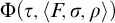 $\Phi (\tau , \langle {F,\sigma ,\rho } \rangle )$
. Then
 $\rho ' = \rho $
.
Proof. By induction on
 $\mathcal {D}$
. We only consider the case for
 $\overrightarrow {\mathrm {Inst}}_{\mathcal {D}}$
, the case of
 $\overleftarrow {\mathrm {Inst}}_{\mathcal {D}}$
will be similar. The only rule which changes
 $\rho $
is an application of Substitution. In this case,
 $\mathcal {D}$
will be of the form

and
 $\overrightarrow {\mathrm {Inst}}_{\mathcal {D}}$
has the form
 $$\begin{align*}\mathrm{S}{\uparrow}[t,s/x] \mathbin{\,{:}\,} \overrightarrow{\mathrm{Inst}}_{\mathcal{D}_1} \mathbin{\,{:}\,} \mathrm{S}{\downarrow}[u,s/x] \end{align*}$$
By assumption we obtain
 $x\notin \operatorname {{\mathrm {dom}}}(\rho )$
as
 $x\in \operatorname {{\mathrm {BVar}}}(\mathcal {D})$
. The i.h. shows that the evaluation of
 $\overrightarrow {\mathrm {Inst}}_{\mathcal {D}_1}$
does not change the assignment. Evaluating
 $\mathrm {S}{\uparrow }[t,s/x]$
changes
 $\rho $
by mapping x to some value, while evaluating
 $\mathrm {S}{\downarrow }[u,s/x]$
removes x from the domain of the assignment. Hence, the resulting overall assignment will be
 $\rho $
again.
The following theorem is a refinement of Theorem 42 in that the claimed existence of update sequences is replaced by an explicit computation based on instruction sequences extracted from the derivation.
Theorem 53 (
$\mathrm {S}^{1}_2 $
).

Let
 $\mathcal {D}$
be a derivation of
 $t = u$
in Variable Normal Form. Let
 $\mathrm {Ax} _0$
consist of those axioms in
 $\mathrm {Ax} $
that occur as injective renamings in
 $\mathcal {D}$
,
 $\rho $
an assignment with
 $\operatorname {{\mathrm {dom}}}(\rho )\subseteq \operatorname {{\mathrm {Var}}}(t,u)$
, and F a
 $\kappa $
-pre-model for
 $\mathrm {Ax} _0$
. Let
 $\sigma _1, \sigma _2$
be given by
 $$ \begin{align*} \langle {F, \sigma_1, \rho} \rangle \quad&=\quad \Phi(\overrightarrow{\mathrm{Inst}}_{\mathcal{D}}, \langle {F, \langle {} \rangle, \rho} \rangle)\\ \langle {F, \sigma_2, \rho} \rangle \quad&=\quad \Phi(\overleftarrow{\mathrm{Inst}}_{\mathcal{D}}, \langle {F, \langle {} \rangle, \rho} \rangle). \end{align*} $$
Then

Instead of proving the theorem directly, we prove the following stronger claim, similar to Claim 43.
Claim 54 (
$\mathrm {S}^{1}_2 $
).

Let
 $\mathcal {D}$
be a derivation in Variable Normal Form. Let
 $\mathrm {Ax} _0$
consist of those axioms in
 $\mathrm {Ax} $
that occur as injective renamings in
 $\mathcal {D}$
. Fix some
 $\kappa $
-pre-model F for
 $\mathrm {Ax} _0$
, and some integer U such that
 ${\mathbf {l}_{0}}(F)+\operatorname {\mathrm {\mathbf {l}}}(\mathcal {D})\le U$
. Let
 $X=\operatorname {{\mathrm {Var}}}(\mathcal {D})$
.
Let
 $\mathcal {D}_0 \vdash t = u$
be a sub-derivation of
 $\mathcal {D}$
. Let
 $\rho $
be an assignment, and
 $\sigma $
a sequence of updates based on
 $F,U$
and
 $\mathrm {Ax} _0$
such that
 $$ \begin{align*} \operatorname{{\mathrm{dom}}}(\rho)\ &\subseteq\ X\setminus\operatorname{{\mathrm{BVar}}}(\mathcal{D}_0) \\ {\mathbf{l}_{0}}(\rho), {\mathbf{l}_{1}}(\sigma), {\mathbf{l}_{0}}(\sigma), {\mathbf{dom}\text{-}\mathbf{l}}(\sigma) \ &\le\ U - \operatorname{\mathrm{\mathbf{l}}}(\mathcal{D}_0). \end{align*} $$
Let
 $\sigma _1, \sigma _2$
be given by
 $$ \begin{align*} \langle {F, \sigma_1, \rho} \rangle \quad&=\quad \Phi(\overrightarrow{\mathrm{Inst}}_{\mathcal{D}_0}, \langle {F, \sigma, \rho} \rangle)\\ \langle {F, \sigma_2, \rho} \rangle \quad&=\quad \Phi(\overleftarrow{\mathrm{Inst}}_{\mathcal{D}_0}, \langle {F, \sigma, \rho} \rangle). \end{align*} $$
Then

Theorem 53 follows from Claim 54 by letting
 $\mathcal {D}_0=\mathcal {D}$
,
 $\rho $
as given,
 $\sigma =\langle {} \rangle $
, and
 $U=\max \{{\mathbf {l}_{0}}(F),{\mathbf {l}_{0}}(\rho )\}+\operatorname {\mathrm {\mathbf {l}}}(\mathcal {D})$
,
Proof of Claim 54.
We argue in
 $\mathrm {S}^{1}_2 $
. Let
 $\mathcal {D}$
, F,
 $\kappa $
, and X be given as in the Claim. We prove that for any
 $\mathcal {D}_0$
,
 $\rho $
,
 $\sigma $
,
 $\sigma _1$
, and
 $\sigma _2$
satisfying the conditions of the Claim, the assertion of the Claim holds, by induction on
 $\operatorname {\mathrm {\mathbf {l}}}(\mathcal {D}_0)$
. Thus this is proven by logarithmic induction (LIND) on a
 $\Pi ^{\mathrm {b}}_{1} $
-property, which is available in
 $\mathrm {S}^{1}_2 $
by Theorem 1.
We consider cases according to the last rule applied in
 $\mathcal {D}_0$
. The details for each case follow the same lines as in the proof of Claim 43, except that now
 $\sigma _1$
and
 $\sigma _2$
are not chosen but given by the
 $\Phi $
-function applied to sequences of instances that are extracted from derivations. Details are left to the reader.
Corollary 55. The consistency of PETS
 $(\mathrm {Ax} )$
is provable in
 $\mathrm {S}^{1}_2 $
.
Proof. We argue in
 $\mathrm {S}^{1}_2 $
. Assume
 $\mathcal {D}$
is a
 $\textbf {PETS} (\mathrm {Ax} )$
derivation ending in
 $0=1$
. Using Proposition 12 we can assume that
 $\mathcal {D}$
is in Variable Normal Form. Let
 $\rho $
be the empty assignment, and F the empty pre-model for
 $\mathrm {Ax} $
. Let
 $\sigma _1$
be given by
 $$\begin{align*}\langle {F, \sigma_1, \rho} \rangle \quad=\quad \Phi(\overrightarrow{\mathrm{Inst}}_{\mathcal{D}}, \langle {F, \langle {} \rangle, \rho} \rangle). \end{align*}$$
By the previous Theorem 53, we obtain

which is impossible.


