

INTRODUCTION
Indices that measure relative abundance of exploited fish species are often based on catch and effort data obtained from commercial and recreational fishers, or less commonly fisheries-independent data such as transect counts from underwater visual census. The use of catch-per-unit-effort (CPUE) to measure changes in stock abundance over time relies on the key assumption that catch rate is proportional to fish density. This relationship can be written as CPUE = qD where D is the population density and q is the catchability coefficient, often defined as the fraction of abundance that is caught by one unit of effort. Ideally q is supposed to be constant which is rarely the case in practice because it is related to the skill and gear efficiency of the fishermen, whereas population density D varies with season and spatial units.
Co-variation between q and D is especially the case for dive fisheries that target sedentary shellfish such as abalone that occur as densely clustered aggregations when stocks are abundant. It is not until targeted aggregations become heavily depleted, and time spent searching for abalone greatly exceeds time spent prising them from the reef surface, that catch rates respond to reduced abundance. In addition, shellfish divers rapidly shift location from reef to reef which makes serial depletion of aggregations difficult to detect (Dichmont et al., Reference Dichmont, Butterworth and Cochrane2000; Hobday et al., Reference Hobday, Tegner and Haaker2001) until conventionally reported effort responds negatively to depletion of the last economically viable aggregations remaining within a statistical reporting area. Compounding the ability of divers to compensate for localized declines in stock is a tendency for abalone to re-aggregate into clusters in response to density reduction (Officer et al., Reference Officer, Gorfine and Dixon2001). This hyper-stability in CPUE is not confined to abalone and has been extensively discussed in past and recent literature (Harley et al., Reference Harley, Myers and Dunn2001; Erisman et al., Reference Erisman, Allen, Claisse, Pondella, Miller and Murray2011; Mogensen et al., Reference Mogensen, Post and Sullivan2014; Maggs et al., Reference Maggs, Mann, Potts and Dunlop2015). Nevertheless, when CPUE is in decline in an abalone fishery there are relatively few alternative explanations apart from stock decline.
Despite its imperfection, CPUE based on commercial catch and effort data is used as an integral part of stock assessments around the world and it is becoming increasingly relied upon as an empirical measure of abundance in Australian abalone fisheries. Use of raw (nominal) CPUE during this process may, however, lead to biased and misleading estimates of relative stock abundance levels because, as we have stated above, raw data can be influenced by many spatiotemporal factors such as area, depth (spatial variability) and season (seasonal variability), and individual anthropogenic factors such as experience and skill of fishers (in our case divers), vessel type and gear efficiency (variability related to the catchability coefficient, q). The process that adjusts for the effects of these factors, using various statistical models, is known as standardization (Gavaris, Reference Gavaris1980; Maunder & Punt, Reference Maunder and Punt2004) and standardization of time-series of data produces yearly trends that within the limitations of the data are more proportional to stock abundance (Shono, Reference Shono2008) or in the case of fishery independent data observable population abundance (Gorfine et al., Reference Gorfine, Forbes and Gason1998).
Perhaps surprisingly given the commonality of standardization, recently it has become a contentious topic among stakeholders, with commercial fishers in some Australian fisheries disputing its use in preference for nominal data. One reason given is that the standardized values are often lower than the nominal arithmetic averages, and less credibly, more nuanced suggestions that trends do not conform to industry aspirations in terms of their financial welfare. Indeed, the inclusion of trends in standardized CPUE and fishery independent abundance as key evidence for over-fished classifications for two of Victoria's abalone fishery management zones (Central and Western) in the 2014 Status of Australian Fish Stocks (SAFS) report (Mundy et al., Reference Mundy, Mayfield, Gorfine, Liggins, Flood, Stobutzki, Andrews, Ashby, Begg, Fletcher, Gardner, Georgeson, Hansen, Hartmann, Hone, Horvat, Maloney, McDonald, Moore, Roelofs, Sainsbury, Saunders, Smith, Stewardson, Stewart and Wise2014) has added to controversy over what to most fisheries scientists should be a fairly simple and routine analytical process. Indeed, despite the addition of two years' data not altering trends in CPUE, the more recent 2016 SAFS report classified these two zones as sustainable (at current low catch levels) and transitional declining respectively, on the basis of a lack of an empirical metric that could unequivocally indicate that an abalone stock was recruitment overfished as defined in SAFS (Mundy et al., Reference Mundy, Stobart, Green, Ferguson, Burnell, Chick, Mayfield, Stewardson, Andrews, Ashby, Haddon, Hartmann, Hone, Horvat, Mayfield, Roelofs, Sainsbury, Saunders, Stewart, Stobutzki and Wise2016).
Statistical models that are most often used to standardize fisheries data include the log-normal regression model, Generalized Linear Model (GLM), Generalized Additive Model (GAM), Linear Mixed Model (LMM) and Generalized Linear Mixed Model (GLMM). Log-normal models are those general linear models where data (usually catch per unit effort, mostly skewed data) are logarithmically transformed to satisfy the assumption of normality with constant variance.
The GLMs are models where the expected value of response variable is linked to the linear combination of explanatory variables by a link function and the response variable can take any distribution from the distribution of the exponential family (McCullagh & Nelder, Reference McCullagh and Nelder1983). Linear Mixed Models and Generalized Linear Mixed Models, both mixed effects models, account for more than just one source of random variability (residual variance). Spatial variability, seasonal variability and variability related to catchability vary across individual CPUE data and hence can be accommodated by fitting appropriate random terms in a mixed effects model without needing to pick a reference level as required in a more conventional model.
Most catch and effort data are collected by fisheries regulatory agencies as a part of the legal compliance requirements imposed on commercial fishermen and not from a scientifically designed sampling regime as would be used for experimental data. This leads to datasets that are highly unbalanced in terms of the number of fishing (sampling) events in each spatial reporting block from year to year. In some instances there may be no catches reported from particular blocks during some years. Unlike conventional linear models, the mixed effects models handle unbalanced data with ease. The advantage of a mixed modelling approach is also described by Candy (Reference Candy2004) who fitted vessel and stratum by year as random effects. The mixed modelling approach for catch and effort is relatively recent and can be found in Cooke (Reference Cooke1997), Rodríguez-Marín et al. (Reference Rodríguez-Marín, Arrizabalaga, Ortiz, Rodríguez-Cabello, Moreno and Kell2003), Brandao et al. (Reference Brandao, Butterworth, Johnston and Glazer2004), Candy (Reference Candy2004) and Tascheri et al. (Reference Tascheri, Saavedra-Nievas and Roa-Ureta2010). The importance of mixed models is reinforced by Venables & Dichmont (Reference Venables and Dichmont2004), who state ‘One of the most important benefits of using mixed models is their capacity to ‘borrow strength’ from one part of the data to another, thus often providing a more realistic analysis of the large fragmentary data sets, which are norm in fisheries research’.
The blacklip abalone fishery in Victoria, Australia is divided into three statutory management zones, Western, Central and Eastern. The Western Zone of the fishery was selected as the subject for this study because a severe outbreak of the lethal disease Abalone Viral Ganglioneuritis (AVG) during 2006–2008 provided an additional source of mortality as a shock against a backdrop of natural and fishing mortality (Mayfield et al., Reference Mayfield, McGarvey, Gorfine, Peeters, Burch and Sharma2011). Although all three sources of mortality are confounded during the 3-year period of co-occurrence, the data span a period that provided five years prior to the disease and six years following its cessation. This facilitated testing the capacity to detect trends across these three different phases of the time series. We used a mixed modelling approach (LMM and GLMM) to produce a time series index of abundance for this Western Zone abalone fishery which was found to be spatially heterogeneous, however we accounted for this heterogeneity by fitting the interaction between spatial region and fishing year as an random effect in the standardizing model.
MATERIALS AND METHODS
Study area
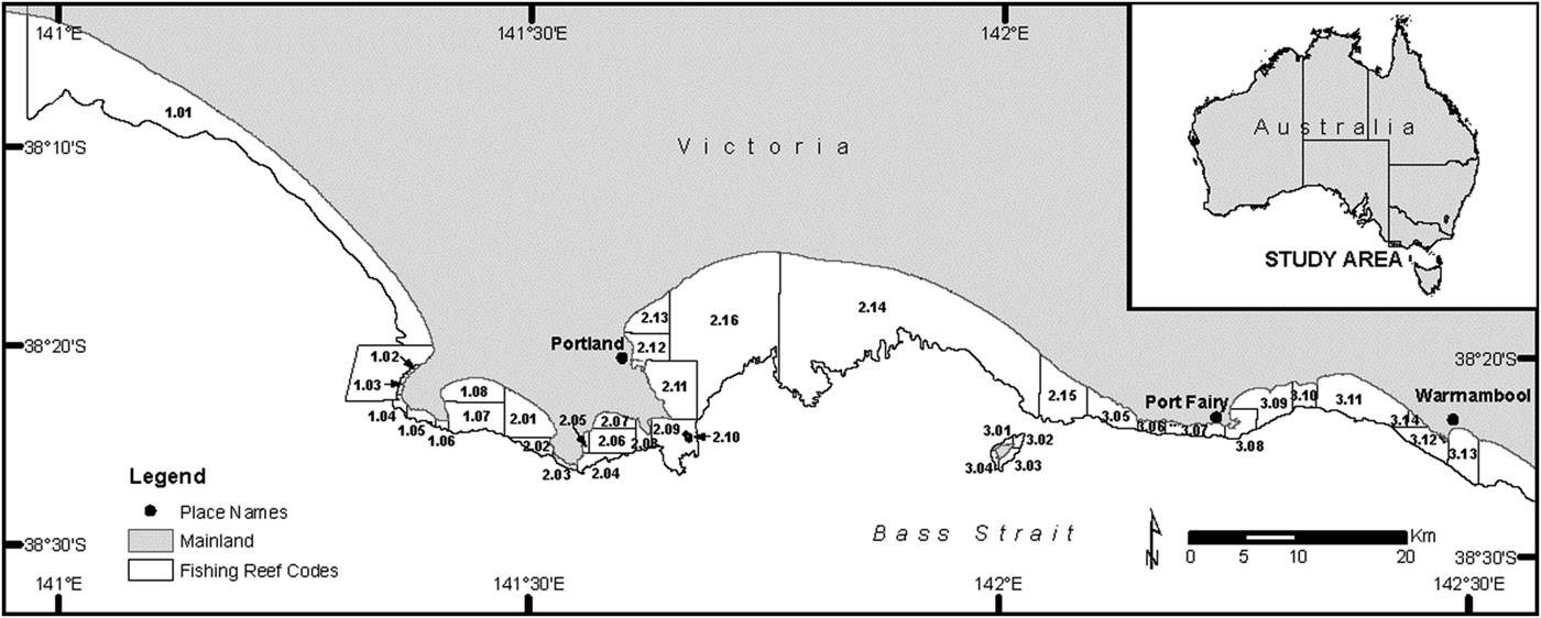
The Western Zone abalone fishery (Figure 1) comprises the region along the south-western coastline of Victoria from the Hopkins River at longitude 142°31′E to the border with South Australia at longitude 140°58′E and 3 Nm seaward, although the fishery almost exclusively operates in depths shallower than 30 msw and blacklip abalone generally do not inhabit reefs deeper than 40 msw.
Disease-affected area in western Victoria, Australia, showing the catch reporting reef code boundaries and the three main seaports used by the Western Zone of the Victorian abalone fishery.

Data
Catch and effort data were acquired consequentially to mandatory reporting requirements for the Western Zone abalone fishery. Within 1 h from the time of landing upon the completion of their period fishing for abalone each day, divers are legally required to provide catch weights (kg) for each reef code visited using an Integrated Voice Response system (IVR) via telephone. Catch weights of whole abalone are determined using certified scales calibrated to 0.1 kg. An abalone docket book unique to each licence holder is also used to document each day's catch and includes additional information such as the fishing effort (h : min) expended taking abalone from each reef code that was visited. There is no regulatory requirement about how effort is measured, which means it could range from a guesstimate to the actual time spent diving as measured by a depth-activated underwater timing device. Effort and other compliance related information is added manually to the catch records captured via IVR. In instances where a diver takes catch assigned to more than one licence a separate IVR report and docket for each licence is required. Daily catch and effort records for individual divers were extracted from the compliance database to enable calculation of CPUE per diver per day per reef code.
Linear Mixed Model
A simple mixed model that describes CPUE, y ijkl from year i, month j, reef code k and diver l, can be given by the equation
 $$y_{ijkl} = \alpha + \gamma _i + m_j + r_k + d_l + \gamma m_{ij} + \gamma r_{ik} + \gamma d_{il} + \varepsilon _{ijkl}$$
where the fixed part of the model consists of α, the overall constant (grand mean) and γ i, the main effect of year i. The random model terms are m j, the effect of month j; r k, the effect of reef k; d l, the effect of diver l; γm ij, the interaction between year i and month j; γr ik, the interaction between year i and reefcode k; γd il, the interaction between year i and diver l; εijkl, the random error term (residual) for unit ijkl.
This mixed model can be written in the matrix form
 $$y = X\beta + Zu + \varepsilon $$
where y, is the vector of observations; β, is the vector of fixed effects with design matrix X; u, is the vector of random effects with design matrix Z; ε, is the vector of the residuals.
The u is normally distributed (Gaussian) centred around zero and the variance  $\sigma _u^2 $. Furthermore it is assumed that u and ε are independent of each other, therefore
 $$\left[{\matrix{u \cr \varepsilon \cr } } \right] \sim N\left( {\left[ {\matrix{0 \cr 0\cr}} \right],\left[ {\matrix{{\sigma _u^2 G} & 0 \cr 0 & {\sigma _\varepsilon ^2 R} \cr}}\right]} \right)$$
where G and R are positive definite matrices that are used to model correlation structures of u and ε.
Parameters in a LMM can be estimated by using Restricted/Residual Maximum Likelihood (REML). The basic premise of a REML algorithm involves partitioning the likelihood into two components and maximizing them separately. The first likelihood component involves all fixed effects parameters and the second likelihood component, known as a residual likelihood, involves the variance parameter of the random effects. The estimated random effects  $\hat u$ are known as the Best Linear Unbiased Predictor or BLUP, also called the ‘shrunken’ parameter estimator, and often BLUP estimates are smaller than those that would have been obtained if they had been fitted as fixed effects. The use of BLUP in estimating random effects in diverse fields of application was highlighted in Robinson (Reference Robinson1991).
This LMM model can easily be extended to a Generalized Linear Mixed Model (GLMM). In GLMM, the CPUE random variable Y i with observed values y i, for i = 1, …, n, is from an exponential family of distributions whose probability density function takes the general form
 $$f\,(y_i\theta _i,\phi ) = {\rm exp}\left\{ {\displaystyle{{y_i\theta _i - b(\theta _i)} \over {a(\phi )}} + c(y_i,\phi )} \right\}$$
where θ is the canonical parameter representing the location, ϕ is dispersion parameter representing the scale and specific functions a(), b() and c() are specified according to various members of the exponential family. The mean of Y i is related to the linear predictor η i by using the link function g where
 $$E[Y_i] = \mu _i = g^{ - 1}(\eta _i),\;\eta _i = g(\mu _i)$$
With canonical link function, θ i = μ i. If β are fixed effects and u represents the random effects, then
 $$\eta _i = x_{i\; \;} ^T \beta + z_i^T u$$
where x i and z i are corresponding rows of design matrices, X and Z for respective fixed and random effects.
Selection of random model
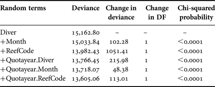
Quota year which starts from 1 April of each year to 31 March of the following year, is fitted only as a fixed effect so that standardized CPUE is easily generated using the yearly coefficient for quota year. The use of quota year rather than conventional calendar year was motivated by a desire to align the standardized CPUE with the total allowable catch (TAC) allocation period which runs on quota year rather than calendar year. The inclusion of terms in the random model was guided by the chi-squared change in deviance test. Deviance is a measure of the goodness of fit of the model to the data such that the smaller the deviance, the better the fit. The contribution made by a term to the fit of the model can be assessed by calculating the change in deviance between two nested models and this change in deviance has a chi-squared distribution with degrees of freedom being equal to the change in degrees of freedom between two models.
Standardized CPUE by marginal prediction
In both the LMM and GLMM models, the standardized CPUE was achieved by generating predicted means (α + γ i) using only fixed effects (year coefficient for each year). By excluding all of the random effects in the prediction, we can say that we have taken the random effects at their population means of zero. Such a prediction method in linear mixed modelling can be termed marginal prediction (Welham et al., Reference Welham, Cullis, Gogel, Gilmour and Thompson2004). Variability arising in CPUE values due to factors such as divers’ skill, seasonal factors and spatial location can be considered to be random variability and thus treated as an error term while forming a predicted value for each year. Unlike conditional prediction where random terms are included by averaging over factors, the marginal prediction is more appropriate when inferences are required for a wider population of random factors. Furthermore, statistical significance of differences was taken when the difference between predicted means for two quota years was greater than 1.96 times the standard error of the difference (SED). Percentage coefficient of variation (% CV) is defined as standard error of mean expressed as percentage of mean ((SE (mean)/mean) × 100).
RESULTS
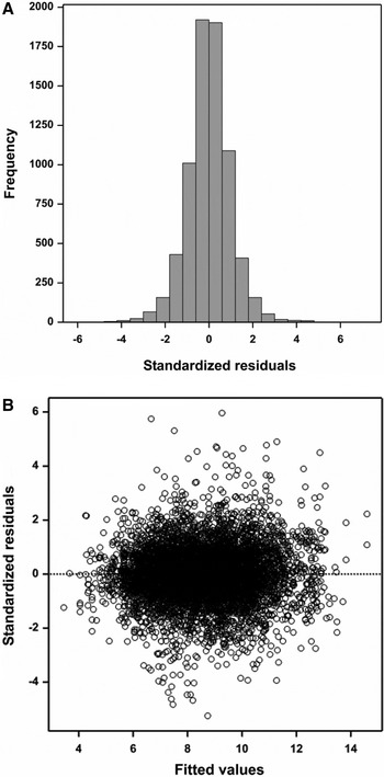
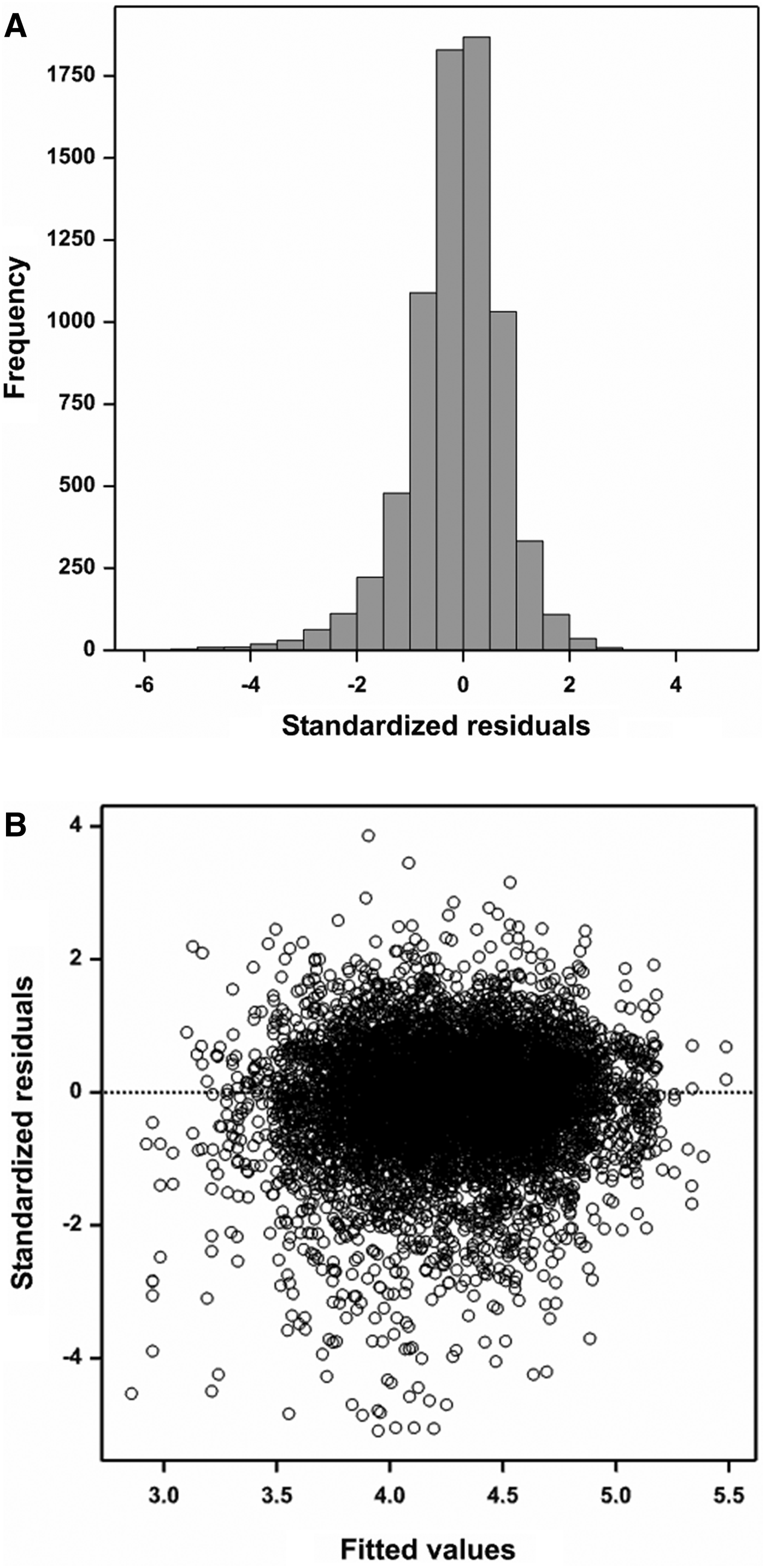
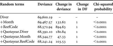
A total of 37 out of 6854 daily diving records resulted in a CPUE of zero, which is about 0.5% of the total diving records in the Western Zone of Victoria. The zero value CPUE records did not show any particular temporal trend, each year having 1–8 with zero values, consequently we excluded these zero values from the remainder of the analyses. There was only one unequivocal instance in which effort was doubly reported due to the catch but not the effort being split between licences, and duplication of records from catch-splitting accounted for only 0.9% of the data and these records were also removed from the analyses. Daily catch (kg) per unit effort (hour) data for each diver per reef (reporting code) was the unit of analysis. Examination of residuals vs fitted values plots from the LMM indicated square root transformation to satisfy the assumption of normality with constant variance as shown in Figure 2. In contrast, untransformed CPUE data (in its original scale) was used in the GLMM with gamma as the error distribution and logarithm as the link function. Selection of the gamma distribution was guided by fitting various continuous distributions to CPUE data and comparing the resulting deviance in each instance. The fitting of the gamma distribution resulted in the smallest deviance, thereby indicating it provided the best fit which may be due to the gamma distribution's capacity to handle skewness in the data. Furthermore, a histogram of residuals (Figure 3A) and a residual vs fitted values plot (Figure 3B) from the GLMM model confirms the appropriateness of the assumption of gamma as the error distribution. Tables 1 and 2 show that the random effects for diver, month and reef code and their interaction with quota year were statistically significant and that the final random model including all of these terms had the lowest deviance for the LMM and GLMM respectively. Consequently we have fitted the same random model structure for the LMM and GLMM.
(A) Histogram of standardized residuals; (B) standardized residuals vs fitted values plot from Linear Mixed Model (LMM).

(A) Histogram of standardized residuals; (B) standardized residuals vs fitted values plot from Generalized Linear Mixed Model (GLMM).

P-values for terms included in the random model for LMM.

P-values for effects included in the random model for GLMM.

Estimated variance components
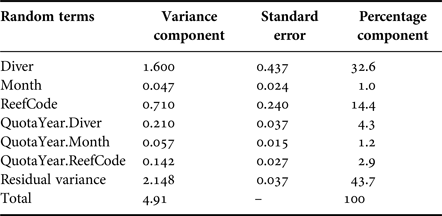
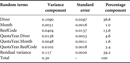
The estimated variance component measures the inherent variability in the CPUE data due to these terms which ranged from 1–37% among the main random effects (Tables 3 and 4). The largest of these among the random terms in the model was the variation due to diver (32.6% in LMM, Table 2 and 36.6% in GLMM, Table 3). This variation reflects differing levels of skill and different fishing practices among divers, and was inconsistent among years as evidenced by the significant diver × year interaction, although accounting for only 4.3% in LMM and 4.6% in GLMM. There was also substantial spatial difference among catch-producing reef areas which accounted for 14.4% of the variation in CPUE in the LMM and 13.6% in the GLMM, and was inconsistent across years (2.9% in LMM and 3.4% in GLMM). The percentage of variability attributable to the combined effect of diver and diver by quota year was higher in the GLMM at 41.2% compared with 36.9% in the LMM. Among random terms, the percentage variability attributable to the combined effects of reef code and reef code by quota year was very similar at around 17% in both the LMM and GLMM. In each model, variability in CPUE due to month and month by quota year was much smaller, accounting for only 2.2% in the LMM and 2.6% in the GLMM. The residual variance of 43.7% was slightly higher in the LMM compared with 39.2% in the GLMM. In both models, the precision with which the variance components are estimated was high with mostly small standard errors apart from the Month effect that nevertheless had only a small variance component.
Estimated random variance components by LMM.

Estimated variance components by GLMM.

Standardized CPUE
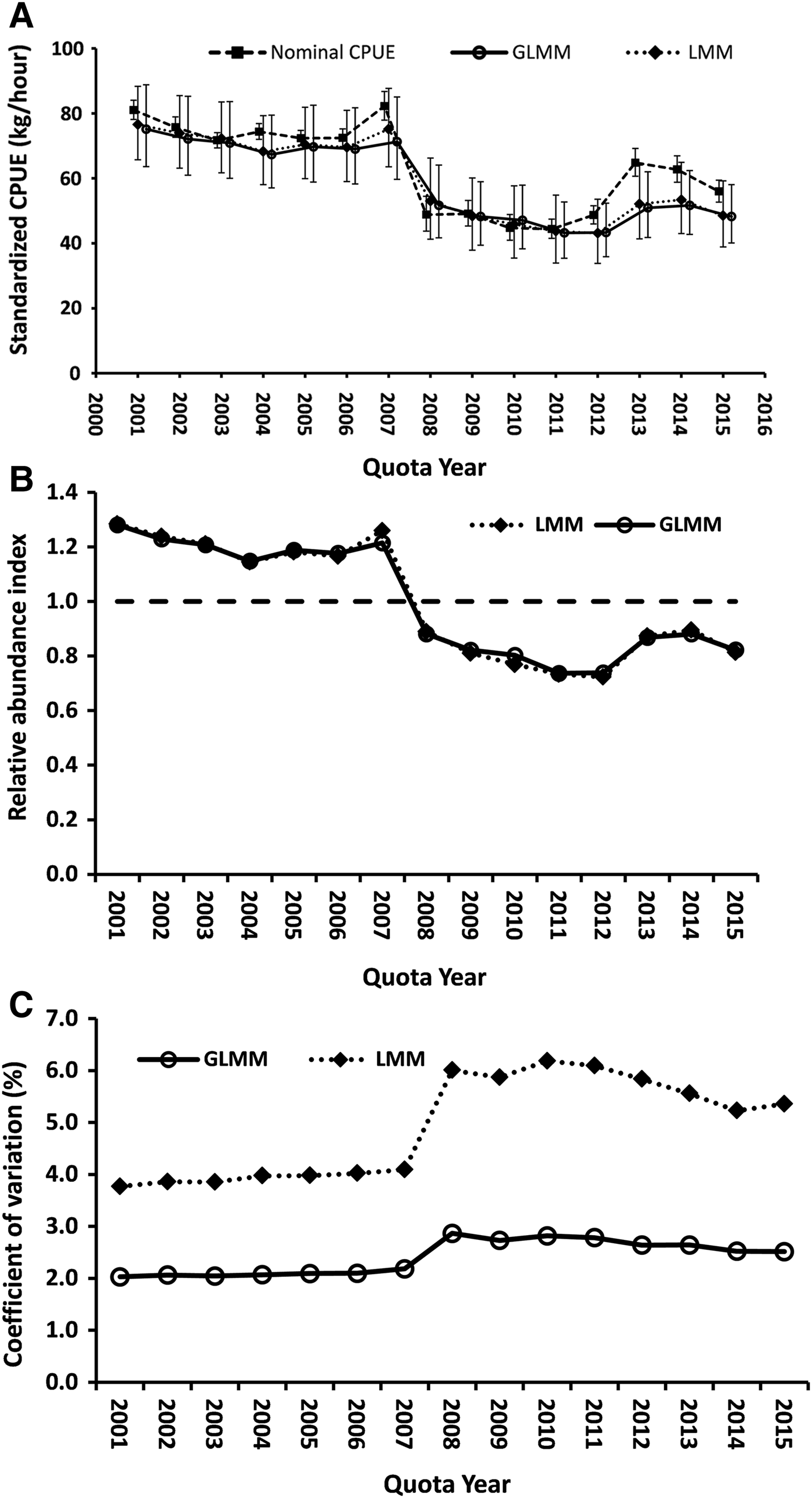
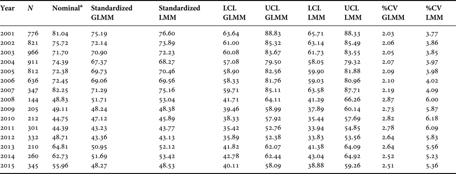
The yearly standardized CPUE values were extracted by generating predicted means for the quota year fixed model term i.e. using coefficients for quota year only. The random effects were not included in the prediction. In other words, the random effects were taken at their population mean of zero. Predicted means were suitably back transformed. It can be seen that the yearly standardized CPUE values from the LMM and GLMM models were almost identical to each other (Figure 4A and Table 5). In both sets of results the standardized CPUE showed a slowly declining trend until the quota year commencing in 2007, after which the trend steepened coincidentally with the occurrence of the outbreak of the abalone AVG virus in Western Victoria. This steeper decline abated during the 2011 quota year and thereafter remained stable without any consistent statistically significant trend upwards despite a progressive but slight numerical increase overall that appears to have levelled out or decreased slightly during the most recent two years of the time series. Although pairwise comparisons based on SED at a 5% level of confidence showed that standardized CPUE values for the quota year 2014 (for both models) were significantly different to the quota year 2012, this was not the case when comparing the values for 2013 and 2015 with 2012. This indicates that more years of data will be required before being able to draw any conclusions with certainty about whether or not stocks in the Western Zone abalone fishery are recovering. Figure 4B presents the inter-annual trend in standardized CPUE divided by the average for the entire standardized time series to create a relative abundance index. This further illustrates that although abundance of the stock shows a slight increase from 2012 level, the value for 2015 remains below the long-term average.
(A) Yearly trend of standardized CPUE compared with nominal CPUE (geometric mean); vertical bars represent confidence limits (B) yearly trend of relative abundance index (yearly standardized CPUE divided by average of entire time series of standardized CPUE); (C) estimated coefficient of variation for standardized CPUE from LMM and GLMM models.

Nominal and standardized CPUEs along with confidence limits and percentage coefficient of variations (%CV).

a Geometric means; LCL, lower confidence limit; UCL, upper confidence limit.
The coefficient of variation (%CV) for yearly estimates of standardized CPUE (in predictor scale) was always lower for the GLMM compared with LMM by a factor of almost one-half (Figure 4C). The maximum difference in %CV is about 3.3% (Table 5) in quota year 2010 and the minimum difference occurred during quota year 2001. As expected, the %CV plot for both models indicates that CPUE values were most variable during the years of disease occurrence, and least at the beginning of the series. During the disease period some reef codes were impacted much more severely than others producing much more variable CPUE than during the earlier disease-free period. The %CV is very slowly decreasing for both models, but it has some way to go to reach the same %CV as the pre-disease period.
DISCUSSION
The substantial proportions of variance attributable to the effects of diver, reef codes and their interaction with year amply demonstrate the need for standardization to detect temporal trends in CPUE for the Western Zone abalone fishery in Victoria. In aggregate these factors accounted for almost 60% of the variation in the data, whereas month and its interaction with year (as a surrogate for seasonal effects such as weather and spawning behaviour) accounted for less than 3%.
The GLMM and LMM produced standardized trends that paralleled and closely approximated each other throughout the series. The GLMM model exhibited smaller residual variance, consequently parameter estimates from the GLMM had better precision than the LMM model. The percentage CV for the GLMM was consistently almost half that of the LMM model. In addition, the combined amount of variation explained by the effects of diver, reef codes, and their interaction with quota year in the GLMM was 4% higher when compared with the LMM. Although both models produced very similar point estimates, the precision of these estimates was better in the GLMM, and on this basis seems to be superior to the LMM in modelling the abalone CPUE data.
The pattern between the nominal and standardized CPUE curves appears similar during the initial 5-year pre-disease period of the series, but from the occurrence of disease in 2006 onward they tend to differ. The standardized curves show a more gradual rate of decline during the disease and post-disease periods than does the nominal curve, with only a slight but mostly non-significant increase at the start of the final three years of the series. The relative abundance index values for recent years are lower than the long-term average of one, indicating that if recovery is actually occurring then the CPUE will take more years to get to the point when it equals the long-term average. It is known that an unbalanced study (unequal number of replications between factor levels) will yield large differences between raw and predicted means because predicted means are weighted more towards those factor levels encompassing most of the observations. Apart from adjusting for the random factors, other plausible explanations about why the nominal pattern differs from the standardized ones relate to spatial shifts in catch, and changes in the fishing pattern and composition among commercial abalone divers in the Western Zone in response to the onset and spread of disease. After the initial detection of active AVG among populations of blacklip abalone adjacent to an abalone farm 6 km west of the township of Port Fairy, the virus spread progressively in both westerly and easterly directions towards the Portland and Warrnambool regions respectively.
Effort mostly shifted towards unaffected reefs as divers fished ahead of the disease. The disease appeared, unsurprisingly, to be more prolific among productive populations of blacklip abalone on reefs with historically higher CPUE. Once the disease had spread to these reefs this led to a progressive increase in the utilization of abalone reefs with inherently lower productivity and commensurately lower CPUE.
Resumption of fishing on disease-affected reefs commenced during 2009 in the form of a structured fishing programme (Peeters, Reference Peeters2011). This programme operated outside the normal quota allocation process and required divers to take catches of 100 kg from within 100–300 m of several specific waypoints during each day's fishing. The rationale was that this would provide information about the extent of disease impact through exploratory fishing within a stratified randomized design. One consequence of this resumption of fishing strategy was that divers were precluded from choosing locations based on pre-disease fishing success and inevitably ended up fishing some parts of reefs with historically low productivity. This could explain at least part of the increase in the nominal CPUE curve after 2011 when the constraints imposed by structured fishing were relaxed and divers were allowed greater choice about where to fish on the disease-affected reefs.
In addition to these changes in fishing practice, changed economic circumstances compounded by global decreases in market prices paid for wild abalone (Gordon & Cook, Reference Gordon and Cook2013) led to a reduction in the number of divers operating on the 14 fishery access licences in the Western Zone (Mayfield et al., Reference Mayfield, Mundy, Gorfine, Hart and Worthington2012). Those divers who remained (about 6–7) tended to be among the more proficient in catching efficiency, which is evidenced in the diver by quota year interaction effect, thereby causing the pattern in unstandardized CPUE to increase.
Standardization of CPUE data for the Western Zone abalone fishery in Victoria, Australia revealed a gradual decline throughout the zone during a 5-year period, steepened by the addition of disease-induced mortality, before levelling out. There is a slight increase in recent years, but more years of data are required before any conclusion can be drawn that blacklip abalone stocks in this fishery are recovering despite stakeholder expressions of optimism that this is occurring.
The use of the mixed modelling approach (LMM and GLMM) was effective as an analytical method for generating an index of abundance in the form of a standardized time series of CPUE for the spatially heterogeneous Western Zone abalone fishery. The GLMM with Gamma distribution seemed to explain more variability in the data and it produced better precision for yearly standardized CPUEs than square root transformed LMM.
A shift in dive-fishing operations towards acquisition of electronically logged and geo-referenced effort, accompanied by intensive electronic measurement of abalone shell lengths in the catch whilst at sea, has occurred in the Western Zone abalone fishery over the decade since the disease outbreak (Ierodiaconou et al., Reference Ierodiaconou, Miller, Rattray, Weeks, Gorfine, Peeters, Van Rooyen, Jalali, Bell and Worthington2014). Sufficient e-data should now be available to undertake a much more refined analysis of CPUE trends including the separation of effort into searching and handling time at fine-scale resolution. Unfortunately, intellectual property considerations and the absence of a regulatory requirement that Industry submit these data to Victorian Government agencies has meant continued reliance on log-book (quota docket) data. It is unsurprising that an industry is unwilling to release data voluntarily when analysis of those data might reveal that a resource upon which it is reliant might not be recovering as well as they had anticipated.
ACKNOWLEDGEMENTS
Thanks are owed to several colleagues at the Department of Economic Development, Jobs, Transport and Resources who provided constructive criticism of the manuscript, in particular Dr Corey Green and Allister Coots who drafted the map of the study area for Figure 1.
FINANCIAL SUPPORT
The senior author undertook the work whilst employed by the Department of Economic Development, Jobs, Transport and Resources, Victoria, Australia in its Agriculture Research Division. The co-author is also employed by the same Department, but his contribution occurred as part of voluntary research activities conducted under the auspices of RMIT University where he holds an unpaid associate position. The study was part of a programme of recurrent State-funded research into abalone stock assessment by Fisheries Victoria, as the State authority responsible for fisheries policy and regulation. Neither author has any commercial interest in the Victorian abalone fishery.