1. Introduction
Buoyancy-driven flows are of paramount importance in various fields such as atmospheric science, oceanography, geology and engineering thermophysics. Although the study of thermal convection has a long history, its nonlinear behaviours, chaotic phenomena and complex boundary conditions continue to reveal a rich external landscape and profound internal physics, persistently igniting the interest and enthusiasm of researchers.
A standard paradigm for studying thermal convection is Rayleigh–Bénard convection (RBC), characterised by heating from the bottom and cooling from the top, resulting in a global temperature gradient that is strictly parallel to gravity (Ahlers, Grossmann & Lohse Reference Ahlers, Grossmann and Lohse2009; Lohse & Shishkina Reference Lohse and Shishkina2024). When this temperature difference is applied along the vertical sidewalls rather than across the top and bottom plates, a related yet distinctly different physical model is formulated. Batchelor (Reference Batchelor1959) referred to this system as the ‘differentially heated cavity’. Because the direction of horizontal heat transfer is orthogonal to the vertical buoyancy flux, it is also known as vertical convection (VC). The motion of fluid confined between two parallel plates in such a system generates the following common control parameters: the Rayleigh number (
 $Ra$
), the Prandtl number (
 $Pr$
) and the aspect ratio (
 $\Gamma$
), which represents the geometrical constraints of the container when considering a confined flow:
 \begin{equation} Ra = \frac {g\beta \Delta TH^3}{\nu \kappa },\quad Pr=\frac {\nu }{\kappa } \quad \text {and}\quad \Gamma =L/H. \end{equation}
Here,
 $L$
denotes the height of the side heated/cooled plate and
 $H$
is the distance between the two parallel plates, with the thermal expansion coefficient
 $\beta$
, the kinematic viscosity
 $\nu$
and the thermal diffusivity
 $\kappa$
.
Currently, a large body of research on turbulent VC has been reported, primarily focusing on various aspects of the system, such as the dynamics of large-scale circulation, small-scale turbulence, boundary layers and global transport (Ng et al. Reference Ng, Ooi, Lohse and Chung2017; Wang et al. Reference Wang, Liu, Shishkina and Lohse2021; Howland, Ng & Lohse Reference Howland, Ng and Lohse2022; Zwirner et al. Reference Zwirner, Emran, Schindler, Singh, Eckert, Vogt and Shishkina2022; Ching Reference Ching2023). A fundamental question runs throughout: understanding and predicting how fluid properties (
 $Pr$
) and the imposed temperature difference (
 $Ra$
) affect heat transport (
 $Nu$
) and turbulence intensity (
 $Re$
). For example, in VC, it was once believed that a universal or single power law could describe the correlation between heat transfer and system parameters,
 $Nu\sim Ra^p$
. However, it has been reported that the exponent
 $p$
depends on
 $Ra$
and may vary between 1/4 and 1/3 (Versteegh & Nieuwstadt Reference Versteegh and Nieuwstadt1999; Yu, Li & Ecke Reference Yu, Li and Ecke2007; Ng, Chung & Ooi Reference Ng, Chung and Ooi2013). Ng et al.’s (Reference Ng, Ooi, Lohse and Chung2015) review of existing data confirmed
 $p \approx 0.31$
, but caution is required when applying pure power-law fits outside the validation range, as it may not provide the best description of the transport relationship.
To address similar issues in RBC and offer a unified perspective, Grossmann & Lohse (Reference Grossmann and Lohse2000) developed the GL theory based on two exact relationships for the dissipation rates of kinetic energy and thermal energy,
 \begin{align} \varepsilon _u=\left \langle \nu (\partial _i u_j)^2 \right \rangle _V=\frac {\nu ^3}{H^4}(Nu-1)RaPr^{-2}, \end{align}
 \begin{align} \varepsilon _T=\left \langle \kappa (\partial _i T)^2 \right \rangle _V=\kappa \frac {\Delta T^2}{H^2}Nu. \qquad \end{align}
The central idea of the theory is to split the kinetic and thermal dissipation rates into contributions from the bulk and boundary layer (BL) in view of the different physics,
 \begin{align} \varepsilon _u= \varepsilon _{u, bulk}+\varepsilon _{u, BL}, \end{align}
 \begin{align} \varepsilon _T= \varepsilon _{T, bulk}+\varepsilon _{T, BL}, \end{align}
and use the characteristic scales of the subregions to derive the corresponding scaling relations through order-of-magnitude approximations. If the separated thermal plumes are considered part of the thermal boundary layer, the plumes and the background flow can replace the previous division (Grossmann & Lohse Reference Grossmann and Lohse2004). In addition to the limiting power laws derived from dominant subregions, inserting the local dissipation expressions into the balance equations yields transport relationships for the entire range, with transitions between different regimes connected by smooth functions (Grossmann & Lohse Reference Davidson2001, Reference Davidson2002). With the expansion of data available for experiments and numerical simulations, Stevens et al. (Reference Stevens, Poel, Grossmann and Lohse2013) determined the prefactors of the GL model more accurately, significantly improving the predictions.
In addition to the original model, the GL theory has achieved great success in other areas, such as inclined convection (Zhang, Ding & Xia Reference Zhang, Ding and Xia2021), horizontal convection (Shishkina, Grossmann & Lohse Reference Shishkina, Grossmann and Lohse2016), internally heated convection (Wang, Lohse & Shishkina Reference Wang, Lohse and Shishkina2021) and double-diffusive convection (Yang & Lohse Reference Yang and Lohse2017). Despite this, its extension to another fundamental model, VC, has encountered considerable difficulties. Ng et al. (Reference Ng, Ooi, Lohse and Chung2015) confirmed that in VC, the inability to obtain an exact expression for the global kinetic dissipation results in an unclosed dissipation balance, hindering the extension of the GL theory. Nevertheless, they found that the scaling of the horizontal buoyancy flux is consistent with the predictions of the GL model. One possible approach to closure is to express the relationship between mean dissipation and mean components using system parameters. Another widely accepted laminar VC scaling theory comes from Shishkina (Reference Shishkina2016), who derived the dependence of
 $Nu$
and
 $Re$
on
 $Ra$
and
 $\textit {Pr}$
through a self-similarity analysis of the Prandtl boundary layer equations, which has been well validated by numerical simulations. This theory will later be used as the standard paradigm for VC scaling and compared with the current results.
In addition to buoyancy, certain externally applied forces may appear as source terms in the Navier–Stokes equation, such as centrifugal and Coriolis forces generated by rotation (Lüdemann & Tilgner Reference Lüdemann and Tilgner2022), or the Lorentz force produced by a magnetic field (Weiss & Proctor Reference Weiss and Proctor2014). In particular, magnetic fields introduce anisotropy, leading to structural changes in the flow dynamics, which gives rise to an additional control parameter: the Hartmann number,
 \begin{equation} Ha = B_0H\sqrt {\frac {\sigma }{\rho \nu }}, \end{equation}
with the electrical conductivity
 $\sigma$
and the density
 $\rho$
.
Typical fluids for studying magnetoconvection (MC) are liquid metals (
 $Pr\sim 10^{-2}$
), with very low viscosity. The resulting strong inertial forces cause the system to develop more quickly into turbulence, manifesting as vortices of various scales. From the perspective of magnetohydrodynamics (MHD), the motion of vortices in a strong magnetic field is mainly controlled by the Lorentz force, with the resulting Joule dissipation leading to a significant reduction in angular momentum perpendicular to the field lines. Meanwhile, global angular momentum conservation must be maintained, and inevitably, the vortices are stretched along the direction of the magnetic field. This pseudo-diffusion of momentum can be seen as the last remnant of Alfvén wave propagation at low magnetic Reynolds numbers (
 $Rm$
) (Davidson Reference Davidson2001a
). In thermal convection of liquid metals, the direction of the external magnetic field relative to the temperature gradient is critical to the flow patterns produced. Two orientations are possible: vertical and horizontal. Taking RBC as an example, a vertical magnetic field strongly suppresses turbulence and increases the critical Rayleigh number for the onset of convection,
 $Ra_c\sim Q$
, where
 $Q=Ha^2$
is the Chandrasekhar number (Chandrasekhar Reference Chandrasekhar1961). As the Hartmann number increases, the flow transitions sequentially from columnar structure to cellular structure, eventually leading to a ‘wall mode’ when convection is strictly constrained (Liu, Krasnov & Schumacher Reference Liu, Krasnov and Schumacher2018; Akhmedagaev et al. Reference Akhmedagaev, Zikanov, Krasnov and Schumacher2020). In the case of stress-free boundaries, the columnar mode exhibits
 $Nu\sim (Ra/Q)$
scaling (Yan et al. Reference Yan, Calkins, Maffei, Julien, Tobias and Marti2019), which has also been verified in two-dimensional (2-D) simulation, and
 $Re\sim RaQ^{-5/6}$
(Bader & Zhu Reference Bader and Zhu2023). In contrast, a horizontal magnetic field induces quasi-two-dimensional (Q2-D) flow structures with convective vortices aligned with the field lines (Yanagisawa et al. Reference Yanagisawa, Hamano, Miyagoshi, Yamagishi, Tasaka and Takeda2013; Vogt et al. Reference Vogt, Ishimi, Yanagisawa, Tasaka, Sakuraba and Eckert2018). The Lorentz force does not affect the critical Rayleigh number
 $Ra_c$
for the onset of convection. Instead, it extends the ‘Busse balloon’ region, where stable convective vortices exist, within a small range of
 $Q$
(Busse & Clever Reference Busse and Clever1983). At this point, the reorganisation of the flow by the magnetic field leads to a significant enhancement of heat and momentum transport. In the optimal state, the convective velocity can even reach the free-fall limit (Vogt et al. Reference Vogt, Yang, Schindler and Eckert2021).
At present, there are two main approaches for considering transport relations in MC. The first is based on the steady-state assumption under the strong
 $Ha$
approximation. This simplifies the complex nonlinear system into a balance between buoyancy and magnetic damping, yielding asymptotically valid scaling relations (Yan et al. Reference Yan, Calkins, Maffei, Julien, Tobias and Marti2019; Tasaka et al. Reference Tasaka, Yanagisawa, Fujita, Miyagoshi and Sakuraba2021). The second extends the GL theory to MC problems, which can be further divided into two subcategories: one focuses solely on identifying the dominant dissipation term, which allows for the derivation of limiting power laws (Bader & Zhu Reference Bader and Zhu2023; Chen, Wang & Ni Reference Chen, Wang and Ni2024); the other involves a generalisation of the full-parameter model similar to the original theory, requiring the additional consideration of Joule dissipation and the introduction of new parameters (Zürner et al. Reference Zürner, Liu, Krasnov and Schumacher2016; Zürner Reference Zürner2020). Recently, Teimurazov et al. (Reference Teimurazov, McCormack, Linkmann and Shishkina2024) proposed a transitional heat transfer model for MC, where the buoyancy-dominated scaling exponent
 $\gamma$
and the Lorentz force-dominated scaling exponent
 $\xi$
are related by
 $\xi =\gamma /(1-2\gamma )$
. The
 $Nu$
results are well supported by DNS and data from the literature.
Here, we focus on the second type of generalised functional relationships, which currently only exist in the RBC model with a vertical magnetic field. Chakraborty (Reference Chakraborty2008) was the first to introduce the concept of a magnetic boundary layer and a magnetic Rayleigh number, resulting in eight regions dominated by either the boundary layer or the bulk. However, the excessive number of free parameters made practical application of the model difficult. Zürner et al.’s (Reference Zürner, Liu, Krasnov and Schumacher2016) pioneering work advanced the development of the theory by identifying four independent regions that distinguish between fully developed turbulence/weakly nonlinear flow and strong/weak magnetic fields. Subsequently, Zürner (Reference Zürner2020) simplified and recalibrated the theoretical model using the latest experimental and numerical data, significantly improving the prediction of
 $Nu$
.
In summary, there is still much work to be accomplished concerning vertical convection. For instance, the extension of GL theory to the classical VC has not yet been fully explored, although some encouraging early outcomes have been obtained. Current attempts in MC are focused on applying a vertical magnetic field, but how the physical picture of the dissipation field would change with the application of a horizontal magnetic field remains to be seen. It is important to note that, in addition to system parameters, the aspect ratio
 $\Gamma$
of the container plays a crucial role in thermal convection for confined flows (rather than between two infinite plates), as it strongly interferes with flow patterns and thereby determines the transport relationships (Shishkina Reference Shishkina2021; Khoubani et al. Reference Khoubani, Mohanan, Augier and Flór2024). For the sake of generality, all simulations in this paper are conducted with
 $\Gamma =1$
. While some similarities are observed with larger aspect ratios, such as
 $\Gamma =3$
or 5, the profiles exhibit complex behaviour (Zwirner et al. Reference Zwirner, Emran, Schindler, Singh, Eckert, Vogt and Shishkina2022), which will be discussed in detail in the following sections.
The present study aims to explore the following questions.
-
(i) What are the physical properties of the dissipation field in vertical convection with low-
 $Pr$
fluids? Do the dissipation scalings from the bulk and the boundary layer conform to the power laws proposed by the GL theory?
-
(ii) How can a reasonable model for global kinetic dissipation in VC be established to close the balance equations? How do the limiting power laws derived from a BL-dominated or bulk-dominated regime compare with existing well-established theories? And how would the full parameter model behave?
-
(iii) If the GL theory can be validated in pure VC, how will the Q2-D flow patterns under an applied horizontal magnetic field affect the global dissipation and the subregion scalings?
-
(iv) Even with the introduction of Joule dissipation, will the potential energy consumption still be dominated by viscous dissipation, similar to Chen et al.’s (Reference Chen, Wang and Ni2024) findings? How valid will the final full parameter model be in describing the transport relations and what are its advantages or limitations?

The remainder of this paper is organised as follows. In § 2, we outline the numerical model and simulation set-up. Section 3 provides a detailed supplement to the classical VC cases without a magnetic field, with § 3.1 summarising the global characteristics and spatial distribution of the dissipation fields. In § 3.2, we examine the
 $Re$
dependence of the dissipation scalings from both the bulk and the boundary layer. Section 3.3 establishes a full-parameter prediction model through a reasonable approximation of global kinetic dissipation and compares it with existing theories. Section 4 is a further extension from the classical VC to the imposed horizontal magnetic field. Section 4.1 summarises the general characteristics of MC and tests the new dissipation relations. In § 4.2, we carefully revise the subregion scalings according to the physical picture of MC. Section 4.3 formulates the total model equations under a horizontal magnetic field, followed by a brief evaluation after fitting the free parameters. In § 5, we discuss several potentially intriguing divergent topics. Finally, the concluding remarks are offered in § 6.
2. Problem statement and formulation
The convection of an incompressible, viscous, conducting fluid in a cubical cavity is considered (
 $\Gamma =1$
). The specific physical properties can be obtained from Zwirner et al. (Reference Zwirner, Emran, Schindler, Singh, Eckert, Vogt and Shishkina2022) (
 $Pr=0.032$
). The set-up follows the standard configuration for vertical convection: the left and right vertical walls are used for heating and cooling, while the other walls are set to be adiabatic. A magnetic field is applied in the horizontal direction along the
 $z$
-axis, perpendicular to the main circulation plane. The Boussinesq approximation is employed to express buoyancy as a linear function of temperature due to density variations. In practical engineering applications, such as a fusion reactor, an induced magnetic field does exist in liquid metal flow, but it is much smaller than the applied magnetic field (
 $Rm=uH/\eta \ll 1$
) and can generally be neglected. Additionally, the contribution of Joule heating is negligible compared with the heat exchange from the isothermal walls. The following three-dimensional dimensionless governing equations are established, where the container height
 $H$
, the free-fall velocity
 $U_f = \sqrt {g\beta \Delta T H}$
, the external magnetic field strength
 $B_0$
and the imposed temperature difference
 $\Delta T = T_h - T_c$
serve as the characteristic scales for length, velocity, magnetic field and temperature, respectively:
(a) Schematic diagram of buoyant convection with a horizontal magnetic field. (b) The
 $xz$
-section parallel to the magnetic field consists of two ‘Side layers’, two ‘Hartmann layers’ and the bulk. (c) The
 $xy$
-section perpendicular to the magnetic field consists of four ‘Side layers’ and the bulk.

 \begin{equation} \nabla \cdot \boldsymbol {u}=0, \end{equation}
 \begin{equation} \frac {\partial \boldsymbol {u}}{\partial t}+(\boldsymbol {u}\cdot \nabla )\boldsymbol {u}=-\nabla p+\sqrt {\frac {Pr}{Ra}}\left(\nabla ^2\boldsymbol {u}+Ha^2(\boldsymbol {j}\times \boldsymbol {e}_b)\right)+T\boldsymbol {e}_y , \end{equation}
 \begin{equation} \frac {\partial T}{\partial t}+\boldsymbol {u}\cdot \nabla T=\frac {1}{\sqrt {RaPr}}\nabla ^2T, \end{equation}
 \begin{equation} \boldsymbol {j}=-\nabla \phi +(\boldsymbol {u}\times \boldsymbol {e}_b), \end{equation}
 \begin{equation} \nabla ^2\phi =\nabla \cdot (\boldsymbol {u}\times \boldsymbol {e}_b), \end{equation}
and
 $\boldsymbol {e}_b$
is the unit vector in the direction of the imposed magnetic field
 $\boldsymbol {B}_0$
. All walls are perfectly electrically insulating and the velocity boundary condition is no-slip.
The cross-sections in the
 $xz$
- and
 $xy$
-planes (figure 1
b,c) contain different flow boundary layers. The Hartmann boundary layer (HBL), whose thickness scales as
 $Ha^{-1}$
, is present on the front and back walls perpendicular to the magnetic field. The side layer, essentially the viscous boundary layer (VBL) under the high-
 $Ha$
asymptote (thickness
 $\sim Ha^{-1/2}$
), exists on the four walls surrounding the main circulation. For both VC and MC, TBL is used to represent the thermal boundary layer. The bulk is typically characterised by the formation of large-scale vortex and recirculation zones, responsible for mixing the fluid and transferring heat. The diagram of the flow subregions presented here serves as an important basis for the subsequent division of the bulk and boundary layer, with care taken to distinguish it from the cases with vertical magnetic field.
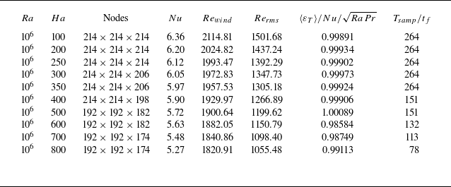
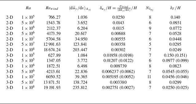
The governing equations (2.1)–(2.5) are numerically solved using a second-order finite volume method, employing a consistent and conservative scheme to compute the current density and Lorentz force (Ni et al. Reference Ni, Munipalli, Huang, Morley and Abdou2007), as discussed in detail by Zhu, Chen & Ni (Reference Zhu, Chen and Ni2024). For the classical VC without a magnetic field, we conduct both 2-D and three-dimensional (3-D) simulations to obtain the necessary data. Table 1 summarises the specific mesh information and reports the Nusselt number, the Reynolds number defined using the ‘turbulent wind’ velocity, and the Reynolds number defined using the root-mean-square (r.m.s.) velocity:
Simulation parameters for pure VC. The columns from left to right indicate the following: dimensionality, the Rayleigh number, the grid resolution
 $N_x\times N_y\times N_z$
, the Nusselt number, the Reynolds number based on maximal vertical velocity, the Reynolds number based on root-mean-square velocity, sampling time. The ‘(uniform)’ case denotes a refined uniform mesh designed to better capture the probability density distribution of the dissipation field, and the rest are non-uniform meshes clustered near the wall. The data in parentheses represent the response parameters obtained from Zwirner et al. (Reference Zwirner, Emran, Schindler, Singh, Eckert, Vogt and Shishkina2022).

 \begin{equation} Nu=\frac {\left\langle \overline {u_xT}-\kappa \partial _x\bar {T}\right\rangle }{\kappa \Delta T/H},\quad Re_{wind}=\frac {\langle \overline {u_y}\rangle _{yz,max}}{\nu /H}\quad \text {and}\quad Re_{rms}=\frac {\sqrt {\langle \boldsymbol {u}\cdot \boldsymbol {u}\rangle _{V,t}}}{\nu /H}. \end{equation}
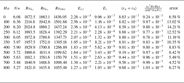
Note that in the 2-D simulations, to obtain the accurate probability density distribution of the dissipation field, we perform additional simulations using very fine uniform grids (listed in table 1, while the rest indicate the non-uniform grids clustered near the boundaries). The 3-D simulations presented here are essentially a reproduction of the work by Zwirner et al. (Reference Zwirner, Emran, Schindler, Singh, Eckert, Vogt and Shishkina2022), but with the added focus on the dissipation field information. To validate the accuracy of the simulations, the response parameters obtained by Zwirner et al. (Reference Zwirner, Emran, Schindler, Singh, Eckert, Vogt and Shishkina2022) are included in the table as a reference. The deviations in
 $Nu$
and
 $Re$
are within
 $1.4\, \%$
and
 $4.2\, \%$
, respectively, indicating a good agreement. More detailed standard deviation of global quantities and validation of the exact relationship for thermal dissipation can be found in table 6 in the Appendix. Figure 2(a) illustrates the local ratio of the 3-D non-uniform grid resolution in the middle
 $xy$
-section to the Kolmogorov scale,
 $\eta _k=(\nu ^3/\varepsilon _{u'})^{1/4}$
. In the centre of the cavity,
 $\Delta _{x,y}\lt 0.8\eta _k$
, while near the wall,
 $\Delta _{x,y}\lt 4.5\eta _k$
. All non-magnetic cases start from an initially stationary field under the given boundary conditions and begin data sampling after no less than 80
 $t_f$
(
 $t_f=H/U_f$
) of development.
(a) Ratio of 3-D non-uniform grid resolution in the middle
 $xy$
-section to Kolmogorov scale (
 $\Delta _{x,y,z}/\eta _k$
) at
 $Ra = 5\times 10^7$
. (b) Grid sensitivity study for MC cases at
 $Ra=10^6$
and
 $Ha=200$
: temperature monitoring of
 $G_1{-}G_4$
from
 $170^3\ \text{to}\ 236^3$
.

For the MC cases with a horizontal magnetic field, we fix
 $Ra=10^6$
and vary
 $Ha=100{-} 800$
. Specific information on the 3-D simulations can be found in table 2. A grid independence test was performed on the base mesh, ranging from coarse to fine (
 $G_1{-}G_4$
), with resolutions of
 $170^3$
,
 $192^3$
,
 $214^3$
and
 $236^3$
, respectively. Taking
 $Ha=200$
as an example, grid G3 achieves a suitable balance between adequate resolution and acceptable computational cost (figure 2
b). Considering the Q2-D characteristics induced by the horizontal magnetic field (i.e. the axial velocity gradient is relatively weak in the core), the number of grid points in the magnetic field direction was appropriately reduced (but not less than 4/5 of the original), ensuring at least six grid points in the Hartmann layer. All cases are validated by the exact relation of thermal dissipation rate, which still holds for the MHD flow. The seventh column of table 2 shows the calculation using (1.3) and in most cases, the discrepancy is less than
 $1\, \%$
.
Simulation parameters for MC with a horizontal magnetic field. The columns from left to right indicate the following: the Rayleigh number, the Hartmann number, the grid resolution
 $N_x\times N_y\times N_z$
, the Nusselt number, the Reynolds number based on maximal vertical velocity, the Reynolds number based on root-mean-square velocity, global thermal dissipation compared with the exact relation (1.3)
 $\kappa (\Delta T^2/H^2) Nu=Nu/\sqrt {RaPr}$
, sampling time. The initial field is the statistically steady non-magnetic flow at the corresponding
 $Ra$
.

3. Classical vertical convection without a magnetic field
3.1. Global characteristics and spatial distribution of the dissipation fields
There is extensive visual material available on VC, highlighting key features such as the self-organisation of thermal plumes into a large-scale circulation (LSC), the stable thermal stratification in the bulk and the increase in small-scale turbulent fluctuations as
 $\textit {Pr}$
decreases. Figure 3 provides additional insight into the spatial distribution of dissipation fields by presenting contour plots of
 $\log _{10} \varepsilon _u$
and
 $\log _{10} \varepsilon _T$
for
 ${\textit {Pr}} = 0.032$
, including both instantaneous and time-averaged fields. The instantaneous kinetic dissipation fields reveal the intense nature of liquid metal convection. As
 $Ra$
increases, extreme dissipation transitions from a ‘sheet-like’ to a finer ‘vortex-like’ structure, with the bulk becoming more chaotic due to disturbances from boundary layer separation flows. The extreme region of the mean field evolves from diagonally aligned, approximately elliptical shapes to more rectangular structures that better conform to the cavity geometry, indirectly indicating the specific morphology of the LSC. Importantly, the distribution of
 $\varepsilon _u$
remains predominantly concentrated within the VBL (both vertical and horizontal). The instantaneous thermal dissipation fields, influenced by the large thermal diffusivity, exhibit coarser plume structures that are advected downstream by the LSC. As
 $Ra$
increases, more small-scale structures extend randomly from the hot and cold plates into the bulk, though the overall spatial scale is significantly larger than the ‘filamentary’ structures observed in RBC at intermediate
 $\textit {Pr}$
(Xu et al. Reference Xu, Wang, Wan and Sun2021; He, Bao & Chen Reference He, Bao and Chen2022). Similarly, in the time-averaged fields, the contribution of plumes is filtered out, with
 $\varepsilon _T$
concentrating near the TBL where the temperature gradients are the largest, consistent with the adiabatic condition imposed on the horizontal boundaries.
Time-averaged and instantaneous kinetic dissipation (
 $\log _{10} \varepsilon _u$
) and thermal dissipation fields (
 $\log _{10} \varepsilon _T$
) for
 $Ra=10^7$
and
 $5\times 10^8$
from 2-D simulations.

(a,b) P.d.f.s of
 $\log _{10} \varepsilon _T$
and
 $\log _{10} \varepsilon _u$
calculated over the whole 2-D cell. Here,
 $\mu$
and
 $\sigma$
are respectively the mean value and standard deviation. The dashed lines mark the log-normal distribution for comparison. (c,d) P.d.f.s of
 $\varepsilon _T$
and
 $\varepsilon _u$
, obtained over the whole cell and normalised with respect to their r.m.s. values. The curves are the best fits of stretched exponential, as given by (3.1).

Figure 4 presents the probability density function (p.d.f.) of the dissipation fields, sampled from at least 50 snapshots after the flow has reached a statistically steady state. It is important to note that the current p.d.f. statistics are based on simulations using a fine, uniform grid, with specific grid details provided in table 1. The original non-uniform grid, with its exponential distribution near the walls, caused data clustering in phase space, actually increasing the weighting of the boundary layer and introducing non-physical information (Xu, Zhang & Xia Reference Xu, Zhang and Xia2024). To avoid this, it is necessary to ensure uniform spatial resolution across the entire field.
Figures 4(a) and 4(b) illustrate the deviation of the log-normalised p.d.f.s from a log-normal distribution, visually depicting the transition of VC from a flow state concentrated at specific patterns at the lowest
 $Ra$
to a progressively more intermittent and random turbulent state. As
 $Ra$
increases, the distribution of low dissipation (left tail) gradually converges, and the central region becomes more aligned with the log-normal curve, similar to findings in existing RBC studies (Zhang, Zhou & Sun Reference Zhang, Zhou and Sun2017; Venugopal, De & Mishra Reference Venugopal, De and Mishra2022). A pronounced shoulder appears in the high-dissipation region (right tail), which is believed to be associated with high-frequency extreme events (plume emissions) in the boundary layer, indicating the developed intermittency of localised dissipation. This is more clearly demonstrated in figure 4(b), where the two inflection points on the right can be used to distinguish between the bulk flow, plumes/mixing layers and the conductive sublayers (Kaczorowski & Wagner Reference Kaczorowski and Wagner2009). In other words, the strong dissipation in the right tail originates from the steep mean gradients near the conducting walls, while the weak dissipation in the left tail is associated with local fluctuations exhibited by the bulk flow.
Figures 4(c) and 4(d) show the p.d.f.s normalised by the root-mean-square values. At the lowest
 $Ra$
, the tail follows an exponential distribution that appears closer to a straight line on a log-linear scale, without any stretching. As
 $Ra$
increases, the tail gradually broadens and extends towards higher amplitudes, corresponding to the small-scale intermittency caused by more active plume dynamics. Emran & Schumacher (Reference Emran and Schumacher2008) proposed fitting the p.d.f. from the most probable amplitude to the tail using a stretched exponential function:
 \begin{equation} p(X)=\frac {C}{\sqrt {X}}\exp(-mX^\alpha ). \end{equation}
For passive scalar dissipation in the two-dimensional limit of large Peclet and Prandtl numbers, the stretched exponent
 $\alpha$
converges to the derived threshold value of 1/3. This functional form has since been widely applied in describing p.d.f.s in various RBC studies. Here, we extend this approach to VC, which shares similar physical characteristics, and obtain a reasonably good fit, with the related parameters listed in the figures. This analysis suggests that, across different thermal turbulence systems (RBC or VC), the instantaneous dissipation fields dominated by plume activity exhibit certain universal properties.
With a basic understanding of the dissipation distribution across the entire field, we can further quantify the contribution from each subregion of the convective cell. The subregions for kinetic dissipation include the vertical boundary layer near the hot and cold walls, the horizontal boundary layer near the top and bottom walls, and the bulk. For thermal dissipation, the subregions consist of the thermal boundary layer and the central bulk. To reasonably distinguish, it is necessary to accurately calculate the boundary layer thickness, which varies depending on the specific thermal turbulence system and boundary conditions. In 2-D RBC, Zhang et al. (Reference Zhang, Zhou and Sun2017) defines the VBL as the location of the maximum r.m.s. velocity to avoid non-physical thickness caused by corner vortices. Zhang, Dong & Xia (Reference Zhang, Dong and Xia2022), in inclined convection, defines the VBL thickness as the
 $x$
-direction position of the maximum vertical velocity. Lim et al. (Reference Lim, Chong, Ding and Xia2019) defines the stress boundary layer thickness as the location of the maximum sum of the velocity normal gradient squares. In VC, since the large-scale turbulent ‘wind’ is easily identifiable, the VBL thickness generally follows the laminar Prandtl–Blasius (P-B) scaling (Ng et al. Reference Ng, Ooi, Lohse and Chung2015). It can be defined as the point where the tangent to the mean velocity profile at the wall equals the turbulent wind velocity (
 $\delta _u = U / ({\rm d}\bar {u}/{\rm d}x|_w)$
), a method also applied in most RBC configurations.
Relatively speaking, the definition of TBL thickness is more consistent, typically employing the slope method, which defines the thickness as the intercept of the tangent to the mean temperature profile at the wall with the horizontal axis (
 $\delta _T = -(\Delta T/2)/({\rm d}\bar {T}/{\rm d}x|_w)$
). Additionally, Howland et al. (Reference Howland, Ng and Lohse2022) defines the conductive TBL in high-
 $Pr$
VC as the wall-normal location where the conductive heat flux equals the turbulent heat flux (
 $-\kappa {\rm d}\bar {T}/{\rm d}x = \overline {u'T'}$
), with the heat flux being dominated by mean molecular diffusion. Ng et al. (Reference Ng, Ooi, Lohse and Chung2015) compared three boundary layer definitions: the tangent intercept method, the dissipation cross-over point and the displacement thickness, demonstrating that the scaling relations were largely consistent,
 \begin{equation} \delta _u /H \approx 0.43Re^{-1/2}, \quad \delta _T /H \approx 2.1Re^{-1/2}. \end{equation}
Following Ng et al. (Reference Ng, Ooi, Lohse and Chung2015), Zwirner et al. (Reference Zwirner, Emran, Schindler, Singh, Eckert, Vogt and Shishkina2022) and Shishkina (Reference Shishkina2016), we adopt the slope method to define the VBL and TBL thickness.
Figure 5 illustrates the percentage of dissipation in each subregion for different
 $Ra$
in the present 2-D simulations. Specific boundary layer information can be found in table 7 in the Appendix. The results indicate that the relative contributions of the VBL and bulk to
 $\varepsilon _u$
remain nearly constant, staying around
 $60\, \%$
and
 $40\, \%$
, respectively. Notably,
 $\varepsilon _{u, BL}$
from the horizontal boundary layer is a significant source of kinetic dissipation, comparable in magnitude to that from the generally considered vertical boundary layer. Additionally, the fraction of both alone is less than the bulk dissipation. As
 $Ra$
increases, the proportion of dissipation in the horizontal boundary layer decreases, though it still exceeds half of that in the vertical boundary layer, even at the highest
 $Ra$
. Also in the current parameter range, the contribution to
 $\varepsilon _T$
is also dominated by the TBL. Although the bulk contribution slightly increases with
 $Ra$
, it remains significantly lower than that of the TBL.
Percentages of the bulk and BL contributions to the (a) kinetic and (b) thermal dissipation rates for different
 $Ra$
at
 $Pr=0.032$
.

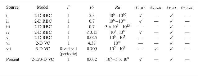
A summary of the dominant subregions for kinetic and thermal dissipation that can be clearly identified from recent publications. The checkmark means that the corresponding dissipation is dominated by this subregion. The sources are as follows: (i, ii) Zhang et al. (Reference Zhang, Zhou and Sun2017), (iii) He et al. (Reference He, Bao and Chen2022), (iv) Zhang & Zhou (Reference Zhang and Zhou2024), (v) Xu, Shi & Xi (Reference Xu, Shi and Xi2019), (vi) Guo et al. (Reference Guo, Wang, Wu, Chong and Zhou2022), (vii) Ng et al. (Reference Ng, Ooi, Lohse and Chung2015).

For ease of reference, table 3 summarises the contributions from the bulk and boundary layer to the kinetic (thermal) dissipation rate that can be obtained clearly from several recent studies on thermal convection. It can be observed that for 2-D thermal convection models with unit aspect ratio, either RBC or VC, both kinetic and thermal dissipation are dominated by the boundary layer across a wide range of parameters. Nonetheless, the local flow organisation in thermal convection systems is strongly correlated with the aspect ratio of the container, and velocity and temperature profiles may exhibit considerably complex behaviour, which has a significant impact on the boundary layer thickness and dissipation statistics in different subregions. For example, Ng et al.’s (Reference Ng, Ooi, Lohse and Chung2015) 3-D VC simulations for a computational domain of
 $8H\times 4H \times H$
found
 $\varepsilon _u$
to be dominated by the bulk and
 $\varepsilon _T$
to remain dominated by the TBL. It might be due to the use of periodic boundary conditions in both directions except for the wall normal phase that the statistics on
 $\varepsilon _u$
includes only the vertical VBL and does not contain the horizontal VBL. Our study indicates that both contribute equally to kinetic dissipation. Additionally, Grossmann & Lohse (Reference Grossmann and Lohse2002) proposed that the theoretical
 $Ra$
scaling of the VBL thickness in RBC aligns more closely with that of the sidewalls rather than the top and bottom plates, suggesting that the main contribution to
 $\varepsilon _u$
appears to come from the sidewalls. For instance, in cylindrical RBC with unit aspect ratio, the contribution from the sidewalls is twice that of the top and bottom combined. Of course, for simplicity, the scaling theory does not distinguish between the positions of the plates and walls in the flow, but instead assumes a characteristic effective thickness in an averaged sense.
3.2. Re dependence of bulk and BL dissipations
Based on the aforementioned statistics of dissipation rates in the bulk and boundary layer, we can examine whether the present low-
 $\textit {Pr}$
VC satisfies the scaling laws proposed by the GL theory. The key relations are briefly outlined as follows:
 \begin{align} \varepsilon _{u,bulk}\sim \frac {U^3}{H}=\frac {\nu ^3}{H^4}Re^3,\quad\qquad \end{align}
 \begin{align} \varepsilon _{u,BL}\sim \nu \frac {U^2}{\delta _u^2}\frac {\delta _u}{H}\sim \frac {\nu ^3}{H^4}Re^{5/2},\qquad \end{align}
 \begin{align} \varepsilon _{T,bulk}\sim \frac {U\Delta T^2}{H}=\kappa \frac {\Delta T^2}{H^2}RePr,\quad \end{align}
 \begin{align} \varepsilon _{T,BL}\sim \kappa \frac {\Delta ^2}{\delta _T^2}\frac {\delta _T}{H}\sim \kappa \frac {\Delta T^2}{H^2}Re^{1/2}Pr^{1/2}. \end{align}
Dissipation scaling laws in the bulk and BL for (a)
 $\varepsilon _u$
and (b)
 $\varepsilon _T$
. A distinction is made between total dissipation (
 $\varepsilon _{u(T), bulk}$
) and fluctuations (
 $\varepsilon _{u'(T'), bulk}$
) in the bulk.

Existing research has provided robust validation of the GL theory for RBC and VC in medium-
 $\textit {Pr}$
fluids, but a common issue persists: while the kinetic and thermal dissipation scaling within the boundary layer can be perfectly reproduced, the contribution from the bulk significantly deviates from the predicted
 $Re$
dependence, with bulk and boundary layer having almost parallel trends. Grossmann & Lohse (Reference Grossmann and Lohse2004) attributed this to the contamination of bulk scaling by plumes detaching from the TBL. Ng et al. (Reference Ng, Ooi, Lohse and Chung2015), however, considered the possibility that turbulent scaling is obscured by the strong mean flow component. Zhang et al. (Reference Zhang, Zhou and Sun2017) proposed that the Kolmogorov energy cascade does not hold in 2-D RBC, as all calculated third-order velocity structure functions are positive.
Figure 6 depicts the trends from the boundary layer and bulk scalings for 2-D simulations. Analogous to the partitioning occupancies demonstrated in figure 5, the boundary layer contributions are in better agreement with the GL predictions, while
 $\varepsilon _{u, bulk}$
maintains a roughly constant proportionality with
 $\varepsilon _{u, BL}$
. Comparatively, the scaling exponent of
 $\varepsilon _{T, bulk}$
is greater than 1/2, indicating that it is less affected by plume contamination, as the higher thermal diffusivity leads to shorter lifetime of local plumes, with fewer chances of penetrating into the bulk. Nevertheless, it is still far from the predicted
 $Re$
dependence. Considering the inherent non-zero mean flow velocity in VC and following Ng et al.’s (Reference Ng, Ooi, Lohse and Chung2015) approach, we subtracted the mean field from the bulk dissipation to isolate the fluctuations for statistical analysis:
 \begin{equation} \langle \varepsilon _{u'}\rangle =\langle \varepsilon _{u}\rangle -\langle \varepsilon _{\bar {u}}\rangle , \quad \langle \varepsilon _{T'}\rangle =\langle \varepsilon _{T}\rangle -\langle \varepsilon _{\bar {T}}\rangle , \end{equation}
where
 \begin{equation} \langle \varepsilon _{\bar {u}}\rangle =\frac {2}{H}\int _{\delta _u}^{H/2}\nu \left(\frac {{\rm d}\bar {u}}{{\rm d}x}\right)^2{\rm d}x, \quad \langle \varepsilon _{\bar {T}}\rangle =\frac {2}{H}\int _{\delta _T}^{H/2}\kappa \left(\frac {{\rm{d}}{\bar {\rm{T}}}}{{\rm d}x}\right)^2\rm{d}x. \end{equation}
The results successfully reproduce the corresponding theoretical scalings, further confirming that in VC, the small-scale turbulent transport driven by the large-scale mean field is consistent with the Kolmogorov framework. Notably, as
 $Ra$
increases, the proportion of dissipation attributed to the mean field (the difference between the solid and hollow triangles in figure 6) gradually decreases, indicating that turbulent fluctuations progressively dominate. This observation mirrors Wang et al.’s (Reference Wang, Liu, Shishkina and Lohse2021) results for high-
 $\textit {Pr}$
VC, although the transition
 $Ra$
in their case is significantly larger.
Time and surface averaged horizontal profiles of (a) the vertical velocity component and (b) the temperature near the heated wall. The dashed line represents the tangent at the centre of the profile.

It should be emphasised that the current treatment is not identical to that of Ng et al. (Reference Ng, Ooi, Lohse and Chung2015), as no additional correction has been made to the characteristic velocity using the midline-averaged gradient. The key distinction lies in the velocity profiles presented in the reference (figure 7 from Ng et al. Reference Ng, Ooi, Lohse and Chung2015), which show a well-developed velocity distribution extending from the near-wall region to the bulk centre up to
 $Ra = 2 \times 10^7$
. The mean velocity obtained from the central gradient is a direct value, closely approximating the maximum velocity of the turbulent ‘wind’. Figure 7 illustrates the surface-averaged velocity profiles acquired in this study. As
 $Ra$
increases, the peak velocity rises sharply and the overall jet becomes more confined near the wall. Meanwhile, the velocity outside the jet, closer to the bulk, drops drastically, with the vertical velocity and temperature in a substantial part of the bulk remaining close to zero. At this stage, the dashed line representing the central tangent in the figure fails to reflect the average velocity or temperature gradient in the bulk. The fundamental cause of this profile discrepancy might be explained by Zwirner et al.’s (Reference Zwirner, Emran, Schindler, Singh, Eckert, Vogt and Shishkina2022) figure 8. It is evident that the closer the aspect ratio is to 1, the more fully mixed the bulk becomes, which is characterised by an isothermal profile close to
 $(T_h +T_c)/2$
and nearly zero vertical velocity. As
 $\Gamma$
increases, the mean gradient at the bulk centre increases. This difference can be confirmed to be weakly related to
 $\textit {Pr}$
, since the current low-
 $\textit {Pr}$
profiles exhibit similar behaviour to those in Wang et al.’s (Reference Wang, Liu, Shishkina and Lohse2021) high-
 $\textit {Pr}$
cases. Despite this, it cannot be determined to be independent of the boundary conditions, as both Ng et al. (Reference Ng, Ooi, Lohse and Chung2015) and Howland et al. (Reference Howland, Ng and Lohse2022) applied a periodic boundary in the streamwise and spanwise directions with an aspect ratio of
 $8\times 4 \times 1$
. In contrast, both the current study and that of Wang et al. (Reference Wang, Liu, Shishkina and Lohse2021) consider a 2-D enclosed model with horizontal no-slip boundaries
 $( \Gamma = 1)$
. The presence of horizontal plates has a crucial influence on VC, primarily through the generation of corner vortex structures. The temperature profiles intuitively display the so-called ‘undershoot’ phenomenon, where the temperature drops below the bulk temperature after descending from
 $T_h$
before oscillating back to the bulk value. This results in the central gradient, as indicated by the dashed line in the figure, being opposite to the mean gradient. The reason for this can be understood as the rate of heat transfer from the wall to the outer boundary layer is not sufficient to keep the temperature synchronised with that of the exterior as the fluid rises vertically (Ravi, Henkes & Hoogendoorn Reference Ravi, Henkes and Hoogendoorn1994). As a consequence, cooler fluid relative to the core appears, descending as it passes through the corners and separating from the horizontal wall, forming additional circulations.
In conclusion, by filtering out the obscuring effect of the strong mean field, we are able to reproduce the classical theoretical scalings. Nevertheless, the influence of the vessel aspect ratio, including boundary conditions, on the local flow structures, profile shapes and related statistics requires additional consideration.
3.3. Modelling of global dissipation and extension to classical VC
The starting point of the GL theory lies in two exact relations for kinetic dissipation and thermal dissipation, (1.2) and (1.3), which can be derived by multiplying the general form of the momentum equation by
 $ u$
, and the temperature transport equation by
 $ T$
, followed by applying Gaussian integration and spatiotemporal averaging under steady-state conditions (Siggia Reference Siggia1994). In fact, the more general relation obtained from the kinetic energy equation is
 \begin{equation} \varepsilon _u=\frac {\nu ^3}{H^4}\frac {\langle u_y T\rangle }{\kappa \Delta /H}RaPr^{-2}, \end{equation}
where
 $ u_y$
is the velocity component in the direction opposite to gravity. This indicates that the buoyant potential energy represented by the vertical heat flux
 $\langle u_yT\rangle$
is converted to kinetic energy and then dissipated by viscous force. In RBC, the heat flux aligns with the buoyancy direction (
 $Nu=\langle u_y T-\kappa \partial _y T\rangle /(\kappa \Delta /H)$
) and (3.9) can be rewritten as (1.2).
In contrast, in VC, the mean horizontal heat flux is orthogonal to the buoyancy direction (
 $Nu=\langle u_x T-\kappa \partial _x T\rangle /(\kappa \Delta /H)$
). Therefore, the exact relationship that links the global dissipation rate to dimensionless parameters no longer holds. Meanwhile, the thermal dissipation rate depends solely on the
 $Nu$
and retains the same form as in the classical case. Thus, designing an accurate global kinetic dissipation model is a key point in extending the GL theory to the context of VC. Currently, there have been some forward-looking and highly valuable studies seeking alternative definitions for this unclosed dissipation relation. For instance, Ng et al. (Reference Ng, Ooi, Lohse and Chung2015) discovered that the horizontal heat flux component satisfies a corresponding scaling and also exhibits a 1/2 power-law in homogeneous VC (Ng et al. Reference Ng, Ooi, Lohse and Chung2018). Zhang et al.’s (Reference Zhang, Ding and Xia2021) successful modelling of the effective horizontal buoyancy in inclined convection is even more encouraging. Despite this, a complete extension of the GL theory to VC and a comparative analysis with existing scaling theories are still lacking at present.
Equation (3.9) informs us that dissipation is proportional to the system’s volume-averaged vertical heat flux,
 $ \langle u_y T \rangle$
. After non-dimensionalising with characteristic velocity
 $ u_0 = (\beta g\Delta TH)^{1/2}$
and temperature
 $ T_0 = \Delta T$
, the kinetic dissipation rate can be written as
 \begin{equation} \varepsilon _u = \frac {\nu ^3}{H^4}\langle u_y^*T^*\rangle Ra^{3/2}Pr^{-3/2}, \end{equation}
where
 $u_y^*$
and
 $T^*$
represent dimensionless vertical velocity and temperature. Taking into account the non-zero mean streamwise velocity in VC, combined with a careful examination of the velocity and temperature profiles, it can be demonstrated that vertical heat flux is primarily concentrated within the TBL (Zwirner et al. Reference Zwirner, Emran, Schindler, Singh, Eckert, Vogt and Shishkina2022), as shown in figure 8(a). As previously mentioned, in the bulk, due to strong flow mixing and thermal stratification, both mean vertical velocity and mean temperature are nearly zero, contributing very little to the overall vertical heat transfer. This phenomenon of concentrated heat flux is remarkably similar to the ‘heat transport channels’ observed in inclined convection, where the temperature and vertical velocity are highly correlated, leading to a significant enhancement in local heat flux. The inset of figure 8(a) shows that the temperature profile converges to 0 much faster despite the larger jet width, i.e. the thickness of the TBL is representative of the actual width of the heat flux (in grey). The following question arises. Can we approximate the total vertical heat flux of the entire field by statistically analysing this portion alone?
(a) Mean vertical heat flux profiles for different
 $Ra$
, where the shaded area of the inset represents the TBL used to approximate statistical kinetic dissipation. (b) Comparison of exact and approximate values of global kinetic dissipation from 3-D DNS, where the inset shows the relative errors. Specific data can be found in table 8 in the Appendix.

The modelling of vertical heat flux within the TBL in this context involves several assumptions or approximations.
-
(i) For low-
$\textit {Pr}$
fluids, the VBL is nested within the TBL and the characteristic velocity has developed into the so-called ‘turbulent wind velocity’. -
(ii) The temperature distribution within the TBL is approximately linear,
$\bar {T}=T_h +{\rm d}\bar {T}/{\rm d}x|_wx$
. -
(iii) The thickness of the TBL is directly defined by the temperature gradient at the plate,
$\delta _T=-(\Delta T/2)/{\rm d}\bar {T}/{\rm d}x|_w$
.


Conditions (ii) and (iii) are evidently valid, as they can be sufficiently verified or analytically derived from the current profiles or published work (Grossmann & Lohse Reference Grossmann and Lohse2004; Ng et al. Reference Ng, Ooi, Lohse and Chung2015). For condition (i), although
 $ u_y$
within the TBL varies, considering the very thin VBL and the fact that the vertical velocity remains close to the ‘turbulent wind velocity’ within the statistical region, it is still feasible to approximate with a constant value. This will naturally lead to an overestimation, but subsequent quantitative comparisons demonstrate that the resulting error is acceptable. An independent approximation of the product of the vertical heat flux is then obtained:
 \begin{equation} \langle u_y^*T^*\rangle \sim u_{wind}^*\left \langle \, T^*\right \rangle \sim \frac {RePr^{1/2}}{Ra^{1/2}}\int _{0}^{\delta _T}\left(1-\frac {x}{\delta _T}\right){\rm{d}}x = \frac {RePr^{1/2}}{4NuRa^{1/2}}, \end{equation}
which results in a fairly reasonable estimate of the global kinetic dissipation in VC (substitute (3.11) into (3.10)),
 \begin{equation} \varepsilon _u=\frac {\nu ^3ReRa}{4H^4NuPr}. \end{equation}
To verify (3.12), the exact and approximate values of kinetic dissipation are examined in 3-D VC simulations (
 $\Gamma =1$
) and the expression (1.2) applied to the RBC is additionally calculated for comparison. As shown in figure 8(b), the exact values are very close to the estimated ones, with the relative error, displayed in the inset, ranging between 6
 $\, \%$
and 28
 $\, \%$
. In contrast, the classical formula (1.2) significantly overestimates the actual dissipation, with errors ranging from 65
 $\, \%$
to 215
 $\, \%$
. In fact, the ratios,
 $\varepsilon _u/(\nu ^3H^{-4}(Nu-1)Ra)$
, measured by Shishkina (Reference Shishkina2016) in a cylindrical container with equal height and diameter, range from 0.2 to 0.6 (
 $Pr = 0.1, Ra = 10^5{-} 10^{10}$
), which are weakly correlated with
 $Ra$
. Similarly, Wang et al. (Reference Wang, Liu, Shishkina and Lohse2021) obtained a ratio of approximately 0.4 in 2-D VC, corresponding to a relative error of approximately 150
 $\, \%$
. All these findings suggest that the classical formula is no longer applicable in VC due to the orthogonality between buoyancy and heat flux.
It is worth cautioning of the error at the highest
 $Ra$
in the current approximation, which cannot be overlooked. This calls for careful consideration of the model’s applicable range. The starting point of the modelling is an approximate statistic of the vertical heat flux, and the corresponding error arises from two main sources. On the one hand, it stems from our choice of a constant Reynolds number: as indicated by the inspection of velocity profiles in figure 7, the jet width narrows sharply with increasing
 $Ra$
, leading to a very steep velocity distribution within the TBL. In this case, using the peak
 $Re$
undoubtedly overestimates the actual vertical heat flux. On the other hand, the concentration of heat flux in the TBL requires the velocity profile to exhibit a full peak near the wall, which should be representative of the overall flow. The 2-D VC velocity profiles with
 $Pr$
= 10 shown by Wang et al.’s (Reference Wang, Liu, Shishkina and Lohse2021) figures 3 and 4 indicate that after
 $Ra$
reaches
 $2\times 10^{11}$
, the horizontal flow, originally concentrated near the top and bottom walls, evolves into a strong horizontal velocity in the bulk as zonal flow. Meanwhile, the peak vertical velocity diminishes due to more active plume dynamics, attenuating the overall vertical motion. At this point, any statistical treatment of the vertical heat flux becomes inaccurate. Moreover, for low-
 $Pr$
fluids (
 $Pr$
= 0.03), the transition
 $Ra$
will undoubtedly occur even earlier.
(a,b)
 $Ra$
dependences of the compensated forms of
 $Nu/Ra^{1/4}$
and
 $Re/Ra^{1/2}$
from Shishkina (Reference Shishkina2016) and Zwirner et al. (Reference Zwirner, Emran, Schindler, Singh, Eckert, Vogt and Shishkina2022). (c,d) Reproductions of Shishkina’s (Reference Shishkina2016) figures 3(b) and 3(d): the
 $Pr$
dependences of
 $Nu$
and
 $RePr$
. The solid lines represent the scalings from (3.14).

Nevertheless, the above approximate model provides a relatively accurate alternative to the global kinetic dissipation statistics of VC under the current parameter range. Below, we apply (3.12) to the extended GL theory and compare the results with existing studies and well-established scaling theories. As shown in figure 5, the dissipation fields in the present simulations are dominated by the boundary layer, allowing for the simplification of (1.4) and (1.5) to obtain an effective pure power-law scaling. The joint equations
 \begin{equation} \frac {ReRa}{NuPr} \sim Re^{5/2} \quad \text {and} \quad Nu \sim Re^{1/2}Pr^{1/2} \end{equation}
are solved as follows:
 \begin{equation} Nu \sim Ra^{1/4}Pr^{1/8}, \quad \quad Re\sim Ra^{1/2}Pr^{-3/4}. \end{equation}
Surprisingly, the scaling (3.14) is identical to the predicted scaling for the
 $I_l$
regime in the unified RBC theory (Grossmann & Lohse Reference Grossmann and Lohse2000), despite the expressions for
 $\varepsilon _u$
being quite different. In comparison to the theoretical scaling obtained by Shishkina (Reference Shishkina2016) based on the Prandtl method,
 \begin{equation} Nu \sim Ra^{1/4}Pr^{1/4}, \quad \quad Re\sim Ra^{1/2}Pr^{-1/2}, \end{equation}
the classical
 $Ra$
dependence can be reproduced, i.e.
 $Nu \sim Ra^{1/4}$
and
 $Re \sim Ra^{1/2}$
. As shown by the compensated quantities from Shishkina (Reference Shishkina2016) and Zwirner et al. (Reference Zwirner, Emran, Schindler, Singh, Eckert, Vogt and Shishkina2022) in figures 9(a) and 9(b), the results agree well with the current derivation and previously established theory. Upon narrowing the vertical axis range, slight fluctuations in the trend become noticeable. In particular, the compensated
 $NuRa^{-1/4}$
increases with
 $Ra$
, which could be due to the geometric constraints of the convective cells affecting heat and mass transfer, or it might suggest a transition towards the
 $Ra^{1/3}$
scaling (
 $Ra \gt 10^7$
, Ching Reference Ching2023). At present, there is insufficient evidence to provide a definitive answer.
It is noteworthy that the current
 $Pr$
exponent is slightly different from the laminar scaling proposed by Shishkina (Reference Shishkina2016). Here, we reproduce figures 3(b) and 3(d) of that article, i.e. the
 $Pr$
dependence within an equal height and diameter cylindrical cell for fixed
 $Ra = 10^6$
and
 $10^7$
in figure 9(c) and 9(d). Interestingly, the scalings
 $Nu \sim Pr^{1/4}$
and
 $Re \sim Pr^{-1/2}$
fit well in the small
 $Pr$
limit (
 $Pr \lt 0.03$
), with a slight overestimation between 0.03 and 1 (especially for
 $RePr$
). In contrast, the current scalings
 $Nu \sim Pr^{1/8}$
and
 $Re \sim Pr^{-3/4}$
, are supported by the data over almost the full range where
 $Pr \lt 1$
. Let us revisit the origins of these two
 $Pr$
scalings: the former is based on an extended Prandtl approach, providing a similarity solution to the heat and momentum transport problem on a vertical heated plate. For the detailed derivation, please refer to the original work (Shishkina Reference Shishkina2016); we briefly outline the method here to facilitate the following analysis.
 \begin{align} u_x\partial _xu_x+u_z\partial _zu_x = \nu \partial _z^2u_x+\beta g(T-T_0), \end{align}
 \begin{align} u_x\partial _xT+u_z\partial _zT = \kappa \partial _z^2T,\qquad\quad \end{align}
 \begin{align} \partial _xu_x+\partial _zu_z=0.\qquad\qquad \end{align}
Note that the
 $x$
direction is along the plate and the
 $z$
direction is horizontal away from the plate. Construct the following similar variable
 $\xi$
, stream function
 $\psi$
and temperature for the Prandtl boundary layer equations (3.16)–(3.18):
 \begin{align} \xi = Pr^aRa^b(z/H)(x/H)^c, \end{align}
 \begin{align} \psi = Pr^dRa^e\nu (x/H)^f\phi (\xi ), \end{align}
 \begin{align} T = T_0+(\Delta T/2)\theta (\xi ). \quad\end{align}
The Nusselt number is obtained from the average temperature gradient at the plate, while the Reynolds number is determined based on the maximum mean velocity (
 $u_x=\partial _z\psi$
),
 \begin{align} Nu = \frac {-H^{-1}\int _{0}^{H}\kappa \partial _zT|_{z=0}{\rm{d}}x}{\kappa \Delta /H}=\frac {-\theta _\xi (0)}{2(c+1)}Pr^aRa^b, \qquad \end{align}
 \begin{align} Re = \underset {z}{\max }\ H^{-1}\int _{0}^{H}u_x{\rm{d}}x = Pr^{a+b}Ra^{b+e}(c+f+1)^{-1}\phi _\xi . \end{align}
Substitute similarity variables into the heat transport equation (3.17),
 \begin{equation} \theta _{\xi \xi }+fPr^{d-a+1}Ra^{e-b}(x/H)^{f-c-1}\phi \theta _\xi =0, \end{equation}
and eliminate half of the parameters by requiring independence from
 $Ra$
and
 $Pr$
,
 \begin{equation} d=a-1,\quad e=b, \quad f=c+1. \end{equation}
Similarly, substituting (3.19)–(3.21) into the momentum equation (3.16) yields
 \begin{equation} Pr^{4a}\phi _{\xi \xi \xi }+Pr^{4a-1}\left[(c+1)\phi \phi _{\xi \xi }-(2c+1)(\phi _\xi )^2\right]-Ra^{1-4b}(x/H)^{-4c-1}\theta /2=0. \end{equation}
Considering the independence of the momentum equation from
 $Ra$
and the existence of a similarity solution with respect to
 $\xi$
,
 \begin{equation} b=1/4, \quad c=-1/4. \end{equation}
Equation (3.26) can be simplified as
 \begin{equation} 4Pr^{4a}\phi _{\xi \xi \xi }+Pr^{4a-1}\left[3\phi \phi _{\xi \xi }-2(\phi _\xi )^2\right]-2\theta =0. \end{equation}
For
 $ Pr \ll 1$
, the first term on the left-hand side of the above equation can be neglected compared with the second term, yielding
 $ a = 1/4$
, with the corresponding scaling as
 \begin{equation} Nu \sim Ra^{1/4}Pr^{1/4}, \quad Re\sim Ra^{1/2}Pr^{-1/2}. \end{equation}
For
 $ Pr \gg 1$
, the first term in (3.28) dominates and
 $a=0$
. In this case,
 \begin{equation} Nu \sim Ra^{1/4}Pr^{0}, \quad Re\sim Ra^{1/2}Pr^{-1}. \end{equation}
The above scalings are well validated in figure 9, and the same similarity solution approach has been successfully applied in deriving the scaling laws for large-
 $Pr$
RBC, i.e.
 $Nu \sim Ra^{1/3}Pr^{0},\ Re\sim Ra^{2/3}Pr^{-1}$
(Shishkina et al. Reference Shishkina, Emran, Grossmann and Lohse2017). Despite this, as mentioned in the article, ‘Since the
 $Pr$
-dependence holds only for very large or small
 $Pr$
, it formally breaks down for intermediate values of
 $Pr$
, which strictly speaking means the absence of the similarity solution’. This deviation is particularly noticeable in the range of
 $Pr = 0.03{-}1$
in figure 9, even though the scaling law remains entirely valid in a broader sense. A careful examination of the data trends in figure 9(c) suggests that the
 $Pr$
exponent
 $ a$
should vary continuously (slow transition from 1/4 to 0 at
 $Pr\lt 1$
, the 1/4 scaling may be more accurately captured when
 $Pr\lt 10^{-2}$
).
For the case of
 $ Pr \lt 1$
(but not significantly smaller), it may not be appropriate to simply neglect the subdominant terms in (3.28), and the exponent
 $ a$
could lie between 0 and 1/4. The
 $Pr$
exponent for
 $Re$
,
 $ a + d = 2a - 1$
, may be less than -1/2. This aligns with the accepted view that, while pure power-law scaling is sufficiently valid, it may not be the optimal description of transport relationships. Returning to the model presented in this paper, the core focus is on the exact dissipation relations in a thermal convection system and the spatial distribution of vertical heat flux, which are connected to the BL-dominated nature of
 $ \varepsilon _u$
and
 $ \varepsilon _T$
. By solving a set of simple coupled equations, the scaling relations can be derived. The
 $Pr$
exponent of 1/8 for
 $Nu$
and
 $-3/4$
for
 $Re$
correspond well with the results for
 $ Pr$
between
 $ 10^{-2}\ \rm{and}\ 10^0$
. This exponent of 1/8 is based on the physical picture of a BL-dominated system and the profile morphology, representing a transition or average between 0 and 1/4 in the intermediate regime.
In fact, our discussion extends beyond this, and further exploration may yield even more interesting results. Although the subject of this paper is on vertical convection in low-
 $Pr$
fluids, we can reasonably make some predictions about the scaling relationships for
 $ Pr \gt 1$
. As discussed by Grossmann & Lohse (Reference Grossmann and Lohse2001) and Zhang et al. (Reference Zhang, Ding and Xia2021) regarding the ‘lower’ and ‘upper’ subregions, for high-
 $Pr$
fluids, the TBL is nested within the VBL. In terms of the profiles, this implies that at the point where the temperature curve converges from
 $ T_h$
to
 $ (T_h+T_c)/2$
, the velocity has not yet developed to the ‘turbulent wind’ velocity, but is instead represented as
 $ U{\delta _T}/\delta _u$
. At this stage, the expression for dimensionless vertical heat flux can be approximately written as
 \begin{equation} \langle u_y^*T^*\rangle \sim \frac {RePr^{1/2}}{Ra^{1/2}}\int _{0}^{\delta _T}\frac {x}{\delta _u}\left(1-\frac {x}{\delta _T}\right){\rm{d}}x = \frac {Re^{3/2}Pr^{1/2}}{24aNu^2Ra^{1/2}}, \end{equation}
where
 $\delta _u \sim a/\sqrt {Re}$
. The scalings shown in figures 9(c) and 9(d) indicate that for fixed
 $Ra$
of
 $ 10^6$
and
 $ 10^7$
, when
 $ Pr \gt 1$
,
 $Nu$
is independent of
 $Pr$
, while
 $Re\sim Pr^{-1}$
. To ensure rigour, we conduct additional simulations using fine grids for fluids with
 $ Pr = 4.3$
(water) and
 $ Pr = 10$
(lubricating oil) under the same parameter conditions to evaluate the corresponding profiles and dissipation field distributions. The results demonstrate that both kinetic and thermal dissipation are also dominated by the VBL and TBL. To avoid distracting from the main focus of this paper, a detailed description of the high-
 $Pr$
VC simulations is provided in the Appendix, though we strongly encourage readers to refer to this section. Similarly, by solving the following equations:
 \begin{equation} \frac {Re^{3/2}Ra}{Nu^2 Pr} \sim Re^{5/2} \quad \text {and} \quad Nu \sim Re^{1/2}Pr^{1/3}, \end{equation}
the corresponding scalings are
 \begin{equation} Nu \sim Ra^{1/4}Pr^{-1/12}, \quad \quad Re\sim Ra^{1/2}Pr^{-5/6}. \end{equation}
Note that when
 $ Pr \gt 1$
, the form of
 $ \varepsilon _{T,BL}$
differs in (3.32) (the exponent of
 $Pr$
). Equation (3.33) compared with (3.30) has the same
 $Ra$
exponent but exhibits a slight difference in the
 $Pr$
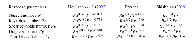
exponent. To clarify this further, table 4 lists several scalings, including the current derivation (3.33), the laminar VC theory (3.30) (Shishkina Reference Shishkina2016) and the effective power laws recently obtained by Howland et al. (Reference Howland, Ng and Lohse2022) from high-
 $Pr$
VC simulations. As shown, the current
 $Pr$
-dependence is more consistent with the results of Howland et al. (Reference Howland, Ng and Lohse2022), with
 $Nu$
showing weak dependence on
 $Pr$
, and the
 $Pr$
exponent of
 $Re$
being slightly greater than -1. Howland et al. (Reference Howland, Ng and Lohse2022) attributes the deviation from laminar VC to the strong turbulence from their set-up, but this can also be explained within the GL framework by the dominant dissipation relationship.
Observed and derived scalings laws for various dimensionless response parameters from large-
 $Pr$
VC. The effective power laws from Howland et al. (Reference Howland, Ng and Lohse2022) for
 $1\leqslant Pr\leqslant 100$
, theoretical scalings for laminar VC from Shishkina (Reference Shishkina2016) and the present scalings are provided for comparison. Note that the following relations exist:
 $Re_{\tau }=H\sqrt {d\bar {u}_y/dx|_{w}}/\nu ^{1/2}$
,
 $C_D=Re_\tau ^2/Re^2$
,
 $C_T=2Nu/(Re_\tau Pr)$
and the Blasius drag law
 $C_D\sim Re^{-1/2}$
.

Overall, whether one starts from Prandtl boundary layer theory or from the exact dissipation relations, both approaches converge on the similar conclusion, showing full harmonisation. The
 $Ra$
dependence of all the response parameters is consistent, while the
 $Pr$
dependence shows slight divergence in applicability. For
 $ Pr \lt 1$
, the current approximation, yielding
 $ a = 1/8$
, provides an averaged characterisation in the intermediate range, which requires the system to be in a VBL–TBL-dominated state, thus imposing certain parameter limitations. If
 $Pr\ll 1$
and
 $Ra$
is extremely large, on the one hand, the VBL becomes extremely thin, potentially leading to
 $\varepsilon _u$
being dominated by the bulk. On the other hand, the high turbulence intensity in the flow field causes the approximate statistic of vertical heat flux to break down. In such cases, the scaling
 $ a = 1/4$
holds true. Currently, research on thermal convection in extremely low-
 $Pr$
fluids is quite scarce (Zwirner et al. (Reference Zwirner, Khalilov, Kolesnichenko, Mamykin, Mandrykin, Pavlinov, Shestakov, Teimurazov, Frick and Shishkina2020),
 $Pr\approx 0.009$
). Determining the critical regimes where different dissipation mechanisms dominate presents a significant challenge, both in terms of computational resources and statistical analysis. For
 $ Pr \gt 1$
, the two sets of scaling relations are also unified and
 $Nu$
exhibits a weak dependence on
 $Pr$
, as the VBL is constrained by the vessel geometry. As
 $Pr$
expands, the flow tends to converge (Grossmann & Lohse Reference Grossmann and Lohse2001). Even so, there are also limitations in terms of
 $Ra$
range, because both the current approximation and boundary layer theory derivations are based on a common core assumption: the buoyancy-driven turbulent ‘wind’ is not strong enough to sustain the turbulent boundary layer in the classical Prandtl and von Kármán sense. As validated by Wang et al. (Reference Wang, Liu, Shishkina and Lohse2021) in 2-D VC simulations with
 $ Pr = 10$
, this transition
 $Ra$
number is approximately
 $ 5 \times 10^{10}$
. Beyond this threshold, the scalings
 $ Nu \sim Ra^{1/3}$
and
 $ Re \sim Ra^{4/9}$
emerge, which are consistent with the predictions of the unified RBC theory in the
 $IV_u$
regime (bulk–bulk dominated). The consistency of the VC scaling with the unified theory suggests a deeper connection between the transport mechanisms in RBC and VC, one that far exceeds previous expectations. This also urges us to treat the conclusions drawn here with great caution.
In the spirit of GL theory, substituting the generalised expressions (3.3)–(3.6) for local dissipation and the approximate statistics of global dissipation into the conservation equations gives the complete functional dependence
 $Nu(Ra, Pr)$
and
 $Re(Ra, Pr)$
, rather than being limited to asymptotic power laws
 \begin{align} \frac {\nu ^3 ReRa}{4H^4NuPr}=c_1\frac {\nu ^3}{H^4}Re^{5/2}+c_2\frac {\nu ^3}{H^4}Re^3, \qquad\qquad \end{align}
 \begin{align} \kappa \frac {(\Delta T)^2}{H^2}(Nu-1)=c_3\kappa \frac {(\Delta T)^2}{H^2}Pr^{1/2}Re^{1/2}+c_4\kappa \frac {(\Delta T)^2}{H^2}PrRe. \end{align}
Compared with the original set of equations applicable to RBC (Stevens et al. Reference Stevens, Poel, Grossmann and Lohse2013), we have the following.
-
(i) The expression for global kinetic dissipation has been modified.
-
(ii) The transition function that represents the cross-over between the VBL and the TBL thickness,
$ f(x) = (1 + x^4)^{-1/4}$
, has been omitted. In fact, integrating this function would be straightforward. Following Grossmann & Lohse (Reference Grossmann and Lohse2001) and Zhang et al.’s (Reference Zhang, Ding and Xia2021) application to smoothing function, dividing (3.31) by (3.11) gives
$Re^{1/2}/(6aNu)=\delta _T/(3\delta _u)$
. Additionally, by setting
$ x = 3\delta _u/\delta _T$
, when
$ Pr \ll 1$
,
$ f(x) \rightarrow 1$
, whereas for
$ Pr \gg 1$
, it approaches
$ x^{-1}$
. Therefore, for the full range of
$Pr$
,
$ \varepsilon _u$
can be expressed as(3.36)The transition in thermal dissipation balance between the bulk and TBL remains the same as in the initial model. Given that our target working fluid is a low-
\begin{equation} \varepsilon _u \sim \frac {\nu ^3 ReRa}{4H^4NuPr}f(6aNuRe^{-1/2}). \end{equation}
$Pr$
fluid (liquid metal) and that modelling for high-
$Pr$
cases is not generally applicable to scenarios where a magnetic field is applied, the function
$f$
is neglected here.
-
(iii) The constraint function
$ g(x) = x(1 + x^4)^{-1/4}$
, which accounts for the saturation of the VBL thickness as it reaches the container scale, has been removed. For the high-
$Pr$
regime,
$Re$
of the large-scale wind decreases as
$Pr$
increases and
$ \delta _u$
gradually grows to its maximum value, comparable to the characteristic scale
$H$
(
$\delta _{u,max}=H/(4\sqrt {Re_c})$
), where
$Re_c$
corresponds to the threshold beyond which a discernible large-scale wind exists in the system. In the case of VC, due to the non-zero mean streamwise velocity, the presence of a turbulent wind is easily identifiable, especially for low-
$Pr$
fluids. Therefore, the function
$ g$
is not necessary within the current parameter range.


Comparison of (a) Nusselt number and (b) Reynolds number data from Shishkina (Reference Shishkina2016) and Zwirner et al. (Reference Zwirner, Emran, Schindler, Singh, Eckert, Vogt and Shishkina2022) (markers) with theoretical predictions (3.34) and (3.35) (lines).

For the coupled equations (3.34) and (3.35), we can use the available data to determine the values of the four priors. Here, four data points from Shishkina (Reference Shishkina2016) (cylindrical cell,
 $ \Gamma = 1$
) and Zwirner et al. (Reference Zwirner, Emran, Schindler, Singh, Eckert, Vogt and Shishkina2022) (square cavity,
 $ \Gamma = 1$
) are chosen to fit the model (the data obtained from the current simulations align closely with those of Zwirner et al. (Reference Zwirner, Emran, Schindler, Singh, Eckert, Vogt and Shishkina2022), as listed in table 1), including
 $Ra=10^5$
,
 $10^8$
at
 $Pr=0.032$
and
 $Ra=10^6$
,
 $10^7$
at
 $Pr=0.1$
. The resulting GL parameters are
 $c_1=6.009, c_2=0.0565, c_3=0.586, c_4=0.00577$
. Note that the coefficients
 $ c_i$
are strictly constrained by the aspect ratio and are not universal. As shown in figure 10, the curves represent the functional relationship described by (3.34) and (3.35) and cover the data points quite well. Strictly speaking, the predicted
 $Re$
at
 $ Pr = 0.1$
slightly underestimates the values at very high
 $Ra$
, which may stem from different cell models (cylinder versus square cavity, and geometric constraints can significantly affect momentum transport) or the critical point for scaling transitions occurring around
 $ Pr = 0.1$
(Shishkina Reference Shishkina2016). Overall, the extended model captures the general trends of
 $Nu$
and
 $Re$
as functions of
 $Ra$
and
 $Pr$
. Additionally, the fitted parameters reveal more insights: the magnitude difference between the bulk and VBL prefactors in the kinetic dissipation balance equation is approximately
 $ 10^2$
. The subregion contributions shown in figure 5 indicate a bulk contribution of approximately 40
 $\, \%$
and a VBL contribution of 60
 $\, \%$
, which are of the same order of magnitude. Considering
 $Re$
values ranging from
 $ 10^3$
to
 $ 10^4$
, the order-of-magnitude difference in the kinetic dissipation expression for subregions (
 $ Re^{1/2} \sim 10^2$
) suggests that multiplying the coefficient by this approximation gives a result that roughly corresponds to the actual partitioning of dissipation. This also aligns with the core principles of the GL theory.
At the end of this section, we would like to briefly evaluate this part of the work. Clearly, the current understanding of transport relationships in classical VC at moderate to high
 $Ra$
is quite mature and comprehensive. The laminar
 $ 1/4$
-power law and the turbulent
 $ 1/3$
-power law are sufficiently effective for practical applications, though the influence of aspect ratio and boundary conditions should not be overlooked. As Ng et al. (Reference Ng, Ooi, Lohse and Chung2015) emphasised, ‘the global kinetic dissipation cannot be determined a priori because the relationship for the buoyancy flux is unclosed’, which can be partially solved by means of a reasonable approximation of the vertical heat flux. Equation (3.36) is essentially appropriate within the range of
 $ Pr = 0.03 {-} 100$
(for moderate
 $Ra$
), and the scaling relations for dissipation in the VBL–TBL-dominant regime have been well validated. Despite this, we are not yet able to make predictions for the other three regimes: VBL–bulk, bulk–TBL and bulk–bulk, due to a lack of fundamental understanding of these issues: the parameter ranges in which they occur, the spatial distribution of dissipation and the behaviour of the profiles, among others. Equation (3.36) cannot be guaranteed to hold in these unexplored regimes. While the VBL–TBL-dominant regime accounts for the majority of results from current simulations and experiments, presenting a complete physical picture of VC under all parameter conditions, with different subregion-dominant regimes, will undoubtedly require much more extensive work.
4. Vertical magnetoconvection with a horizontal magnetic field
This section will further extend the study to VC under the influence of a horizontal magnetic field. Clearly, due to the action of the Lorentz force, the transport relationship governed by a single power law is inherently limited.
As mentioned in § 1, Zürner et al.’s (Reference Zürner, Liu, Krasnov and Schumacher2016) work on scaling theory for vertical magnetic field RBC represents a pioneering extension of GL theory into the field of MC. Even more encouraging is Teimurazov et al.’s (Reference Teimurazov, McCormack, Linkmann and Shishkina2024) development of a parameter-free unified model, which, based on the concept of boundary layer cross-over and the critical Rayleigh number derived from linear stability theory, established a concise and robust set of scaling relations. Nevertheless, this approach is clearly more challenging to extend to VC. The transport relationships for horizontal magnetic field VC were first described by Okada & Ozoe (Reference Okada and Ozoe1992),
 $\widetilde {Nu}=f(Ha/Gr^{1/3})$
, and later validated across a wider range of parameters and under specific boundary conditions (Zhu et al. Reference Zhu, Chen and Ni2024). However, whether it can be incorporated into the framework of GL theory remains an open question.
4.1. Flow characteristics and global relations in a horizontal magnetic field
Isosurface of
 $Q_{c}=0.5\times (|\!|A|\!|_F^2-|\!|S|\!|_F^2)$
(the second invariant of the velocity gradient tensor,
 $S$
is a symmetric tensor and
 $A$
is an antisymmetric tensor), represents the roll structures, coloured by local temperature: (a)
 $Ra=10^6$
and
 $Ha=0$
; (b)
 $Ha=100$
; (c)
 $Ha=400$
; (d)
 $Ha=800$
.

Before expanding on the theory of MC, it is essential to first develop a basic understanding of the flow structure. Figure 11 illustrates the evolution of the vortex structure: when no magnetic field is applied (
 $Ha$
= 0), the flow exhibits a certain degree of isotropic turbulence, although the global circulation can still be vaguely identified. The bulk contains various small-scale structures, with corner vortices breaking up and being stretched along the flow direction due to the entrainment imposed by the mean flow. This will further result in irregular deformation of the cross-section of the main vortex. After the initial magnetic field is applied (
 $Ha$
= 100), the flow develops clear anisotropy. The side vortices are elongated along the field lines without significant interruptions. The vortex surface becomes smoother, and small-scale complex structures are constrained, though some 3-D features remain, such as weak local instabilities between side vortices, intrinsic deformation of the primary vortex and global oscillations induced by the entrainment of side vortices. With a further increase in the magnetic field (
 $Ha \gt 400$
), the flow transitions into a more pronounced Q2-D state. The primary and side vortices become independent and strictly align along the field lines, forming a more coherent and improved self-organised large-scale circulation. Of interest are the two modes exhibited by the flow oscillations: first, the local oscillation of the corner vortex (recirculation region) itself and, second, the more pronounced global elliptical deformation of the main vortex accompanied by the entrainment effect of the corner vortex. The latter diminishes as
 $Ha$
increases, eventually reaching an approximate steady state, but this does not imply the complete disappearance of the corner vortex. As confirmed by our previous study (Zhu et al. Reference Zhu, Chen and Ni2024), the phenomenon of flow separation in weakly nonlinear or laminar flows under the influence of a magnetic field is jointly regulated by magnetic damping effects and the curvature of boundary layer transitions.
The definition of the Q2-D state can be quantitatively described by the correlation of physical fields. In the electrode-driven flow (Potherat & Klein Reference Potherat and Klein2014; Chen et al. Reference Chen, Potherat, Ni and Moreau2021), which is a typical paradigm for the study of MHD turbulence, the strength of the imposed magnetic field can control the flow’s dimensionality (with vortices either partially or fully extending across the cavity). For a given vortex structure with a transverse scale (
 $l_\perp$
), the time required for it to be stretched by the magnetic field to a specific longitudinal scale (
 $l_\parallel$
) is
 \begin{equation} \tau _{2D}=\frac {\rho }{\sigma B^2}(\frac {l_\parallel }{l_\perp }). \end{equation}
Also consider the characteristic motion time of the vortex structure, i.e. the vortex turnover time,
 \begin{equation} \tau _{u}=l_\perp /u(l_\perp ). \end{equation}
When the two are equal, the characteristic scale of the given structure along the magnetic field direction can be determined,
 \begin{equation} l_\parallel = \sqrt {N}l_\perp , \end{equation}
where
 $N=\sigma B^2l_\perp /\rho v(l_\perp )$
denotes the interaction parameter based on the scale
 $l_\perp$
and the velocity of motion
 $v(l_\perp )$
. Considering the spatial scale of the flow region along
 $B$
to be
 $h$
:
-
(i)
$l_\parallel \gg h$
, the flow structure is strictly Q2-D; -
(ii)
$l_\parallel \gtrsim h$
, the flow exhibits weak-3-D characteristics, where the 2-D ‘slices’ along the magnetic field direction maintain approximately equivalent flow topology, but the flow intensity varies significantly due to the influence of the wall; -
(iii)
$l_\parallel \ll h$
, the flow manifests itself as a strong 3-D effect at different locations along the field lines.


Therefore, large-scale structures can reach the Q2-D state more quickly compared with small-scale structures. This can be quantitatively assessed by measuring the correlation at the Hartmann layer, which is fully aligned with the field lines. The correlation functions are given by the following:
 \begin{align} C_1^{\prime}(x, y)=\frac {\sum _{t=0}^{T}\phi _f(x, y, t)\phi _b(x, y, t)}{\sqrt {\sum _{t=0}^{T}\phi _f^2(x, y, t)\sum _{t=0}^{T}\phi _b^2(x, y, t)}}, \end{align}
 \begin{align} C_2^{\prime}(x, y)=\frac {\sum _{t=0}^{T}\phi _f(x, y, t)\phi _b(x, y, t)}{\sum _{t=0}^{T}\phi _f^2(x, y, t)}, \qquad\end{align}
where
 $\phi$
represents the physical field used for statistics, which may include velocity, electric potential, and subscripts
 $f$
and
 $b$
denote the front and back walls. According to Potherat & Klein (Reference Potherat and Klein2014), when strong 3-D characteristics are present,
 $ C_1^{\prime}$
is not equal to 1, but it cannot identify weak 3-D characteristics. For
 $ C_2^{\prime}$
, as long as there is any 3-D effect – whether weak or strong – the value will deviate from 1. In the current cases, note that MC differs from a unilaterally driving of electrode injection flow, as buoyancy as a driving force actually acts over the entire field. In the absence of a magnetic field, instability is triggered by gravitational internal waves generated at separation points or strong shear in the vertical boundary layer (Khoubani et al. Reference Khoubani, Mohanan, Augier and Flór2024). Due to the constraint of the no-slip walls, the highest convective intensity occurs near the centre. The magnetic field, on one hand, eliminates any parallel gradients, and on the other, attempts to smooth the convective intensity along the field lines to minimise wall effects, confining viscous effects to the extremely thin Hartmann layer.
(a) Time- and surface-averaged horizontal profiles of the vertical velocity for different
 $Ha$
near the heated wall. (b) Correlations of the velocity components between front and back Hartmann layers (
 $z_{1, 2}$
) or the Hartmann layer and the centre (
 $z_{1, 3}$
), averaged over several groups.

Thus, in figure 12(b), in addition to measuring the velocity correlations within the relative Hartmann layers (
 $ z_1 = H/Ha,\ z_2 = H(1-1/Ha)$
), it is also necessary to consider the correlation values at HBL relative to the central position (
 $ z_3 = H/2$
) to capture the presence of weak 3-D characteristic. As shown, after the initial magnetic field is applied, the flow structures along the field lines always exhibit
 $C_1^{\prime}\approx 1$
, indicating the absence of strong 3-D, and the convective vortex topology remains self-similar. However, the features of weak 3-D are quite apparent. The values of
 $C_2^{\prime}|_{z_{1, 3}}$
, measured between the near-wall and central region, increase from 0.3 to 0.4 and converge to 0.8 as
 $ Ha$
increases, suggesting non-uniform convective intensity along
 $ B$
and possible 3-D characteristics in small-scale structures. Additionally, due to the symmetry imposed by the no-slip walls,
 $C_2^{\prime}|_{z_{1, 2}}$
is also close to 1 (not shown in the present work). So, we can infer that before
 $C_2^{\prime}|_{z_{1, 3}}$
approaches saturation, the flow is in a ‘weak 3-D’ state, where large-scale Q2-D structures coexist with small-scale 3-D structures. After
 $ C_2^{\prime}$
reaches convergence, the flow transitions into a more complete ‘strong Q2-D’ state. At the present
 $ Ra = 1 \times 10^6$
, this critical
 $ Ha$
lies between 400 and 500. The vortex structures shown in figure 11 provide a more intuitive insight of this discussion on flow dimensionality, setting the stage for the dissipation scaling discussion in § 4.2.
However, in conjunction with the flow images, it is worth emphasising the ‘rectification’ effect of the horizontal magnetic field, i.e. a slight enhancement in convective strength and heat transfer rate at small
 $Ha$
(
 $Nu$
increases by
 $4.93\, \%$
at
 $Ha=100$
, as listed in table 5). This process aligns with the inverse energy cascade observed in classical two-dimensional turbulence, where energy moves from the forcing scale to larger-scale structures (Baker et al. Reference Baker, Potherat, Davoust and Debray2018). Specifically, the magnetic field supports system-size flow by directing the energy of small vortices upward towards the primary vortex. From the perspective of flow coherence, this can be interpreted as an increase in horizontal heat transport per unit area by the plumes, essentially generating better-organised, higher-energy clusters of hot and cold plumes (Zhu et al. Reference Zhu, Chen and Ni2024). Figure 12(a) shows the mean vertical velocity profiles (near the heated wall) at
 $Ra=10^6$
under different
 $Ha$
. It can be seen that at
 $Ha=100$
, the velocity of the ‘turbulent wind’ increases by
 $10.28\, \%$
compared with the profile without magnetic field, indicating that the rectification effect enhances the main circulation by suppressing small-scale 3-D structures. As
 $Ha$
increases further, the Hartmann braking due to magnetic damping intensifies. If flow coherence cannot continue to improve, the convective intensity decreases as dissipation increases.
Response parameters for MC with a horizontal magnetic field. From the sixth column from the left to the last column on the right indicate the following: the average kinetic energy of the main circulation, the kinetic energy along the field lines, total dissipation, the approximate expression (3.12), the relative errors.

Recalling the momentum equation (2.2), the additional Joule heating effect contributes to the dissipation due to the Lorentz force. Apply a similar treatment as in the previous section to obtain the kinetic energy equation
 \begin{align} \frac {\partial }{\partial t}(\frac {u^2}{2})&=-\boldsymbol {\nabla }\cdot \left[\left(p+\frac {u^2}{2}\right)\boldsymbol {u}\right]+\nabla \cdot (u_i\tau _{ij})-2\sqrt {\frac {Pr}{Ra}}S_{ij}S_{ij}\notag\\&\quad+Ha^2\sqrt {\frac {Pr}{Ra}}(\boldsymbol {j}\times \boldsymbol {e}_b)\cdot \boldsymbol {u}+u_yT, \end{align}
where
 $S_{ij}$
is the strain-rate tensor and
 $\tau _{ij}$
is the viscous stress. Taking volume averaging under steady-state condition omits the non-constant term and the divergence term to obtain the equilibrium relationship between potential energy and dissipation,
 \begin{equation} u_yT=2\sqrt {\frac {Pr}{Ra}}S_{ij}S_{ij}-Ha^2\sqrt {\frac {Pr}{Ra}}(\boldsymbol {j}\times \boldsymbol {e}_b)\cdot \boldsymbol {u}. \end{equation}
The work done by the Lorentz force can be rewritten as
 \begin{equation} -Ha^2\sqrt {\frac {Pr}{Ra}}(\boldsymbol {j}\times \boldsymbol {e}_b)\cdot \boldsymbol {u}=Ha^2\sqrt {\frac {Pr}{Ra}}(\boldsymbol {u}\times \boldsymbol {e}_b)\cdot \boldsymbol {j}=Ha^2\sqrt {\frac {Pr}{Ra}}j^2-\boldsymbol {\nabla }\cdot (\phi \boldsymbol {j}). \end{equation}
By removing the divergence terms from the global perspective, we obtain the expression for Joule dissipation under the quasi-static assumption,
 \begin{equation} \varepsilon _b = Ha^2\sqrt {\frac {Pr}{Ra}}j^2, \end{equation}
which can also be written in general form as
 \begin{equation} \varepsilon _b = \frac {\eta }{2}(\partial _ib_j+\partial _jb_i)^2. \end{equation}


Clearly, the exact relationship (4.7) reflects that in MC, the buoyant potential energy (left-hand side) is entirely consumed by kinetic dissipation (first term on the right-hand side) and the work done by the Lorentz force (second term on the right-hand side). This should hold rigorously. The modelling of the total potential energy on the left-hand side can still follow the approximate expression we used for the non-magnetic case (3.12), as the energy source remains unique and definite – the vertical heat flux. Furthermore, the topology of the velocity and temperature profiles is essentially equivalent to that in the absence of a magnetic field, meaning the core argument that ‘vertical heat flux is primarily concentrated within the thermal boundary layer’ remains valid under the current parameters. Consequently, the dissipation relationship (1.2) and (1.3) can be written as
 \begin{align} \varepsilon _u+\varepsilon _b=\frac {\nu ^3}{H^4}\frac {\langle u_y T\rangle }{\kappa \Delta /H}RaPr^{-2}\sim \frac {\nu ^3ReRa}{4H^4NuPr}, \end{align}
 \begin{align} \varepsilon _T=\kappa \frac {\Delta T^2}{H^2}Nu. \qquad\qquad\qquad \end{align}
The conservation relation for thermal dissipation has already been verified in table 2 of § 2. Figure 13 presents the validation of the balance equation and the approximate relation (4.11), with the original equation (1.2) also included for comparison. As expected, the exact balance between potential energy and total dissipation is reproduced, and the approximate expression (3.12) aligns reasonably well with the total potential energy, with an error of approximately
 $ 14.2 \, \%$
at
 $ Ha = 200$
, decreasing to
 $ 4.5\, \%$
as
 $ Ha$
increases. The error observed at low-
 $Ha$
might be attributed to the residual unsteady characteristics of the flow, which transitions to a steady laminar state under a strong magnetic field. In contrast, the expression applicable to RBC shows a significantly larger deviation.
Before examining and adjusting the scaling relations of each component in the bulk and boundary layer, a fundamental issue needs to be reconsidered: the definition of the Reynolds number. In non-magnetic VC, it is typically to define the Reynolds number by the ‘turbulent wind’ velocity (
 $Re_{wind} = HU_{wind}/\nu$
) because the non-zero mean flow is easily identifiable, aligning with the basic assumption in GL theory that a large-scale wind exists. However, in practical applications of thermal convection, the definition of
 $Re$
is not fixed, but tailored to the specific physical model and flow image. For instance, the r.m.s. definition of
 $Re=H\sqrt {\langle \boldsymbol {u\cdot u}\rangle _{V, t}}/\nu$
has been widely used in validating RBC scaling relations (Emran & Schumacher Reference Emran and Schumacher2015; Scheel & Schumacher Reference Scheel and Schumacher2016; Zhang et al. Reference Zhang, Zhou and Sun2017), and applied in extending GL theory to double-diffusive convection (Yang & Lohse Reference Yang and Lohse2017). In MC research,
 $Re_{rms}$
is commonly adopted to provide a measure of the overall flow intensity (Zürner et al. Reference Zürner, Liu, Krasnov and Schumacher2016; Lim et al. Reference Lim, Chong, Ding and Xia2019; Yan et al. Reference Yan, Calkins, Maffei, Julien, Tobias and Marti2019; Akhmedagaev et al. Reference Akhmedagaev, Zikanov, Krasnov and Schumacher2020; Zürner et al. Reference Zürner2020; Nicoski, Yan & Calkins Reference Nicoski, Yan and Calkins2022). Grossmann & Lohse (Reference Grossmann and Lohse2002) proposed that
 $Re$
can be rescaled by any factor without affecting the results for
 $Nu$
, as the shape of
 $Re$
as a function in phase space remains the same, aside from a constant shift. Despite this, Wang et al.’s (Reference Wang, Liu, Shishkina and Lohse2021) results suggest that different definitions of
 $Re$
lead to different scaling relations. To obtain a definition of
 $Re$
suitable for revising the scaling relations, we start with the subregion contributions derived from the conservation of thermal dissipation, which remains invariant in form, and test (3.5) and (3.6).


Figure 14 illustrates the
 $Re$
dependence of thermal dissipation in the bulk and TBL with respect to two different definitions. It can be observed that when the r.m.s. definition of
 $Re$
is used, the classical scaling relations (3.5) and (3.6) are reproduced. In contrast, using the ‘turbulent wind’ definition results in a stronger
 $Re$
dependence (with exponents of 1.52 and 1.94), since the reduction in
 $ Re_{wind}$
is much smaller than that of
 $ Re_{rms}$
as
 $Ha$
increases. This stronger dependence can be explained by the rectification effect of the horizontal magnetic field discussed earlier: the main circulation is enhanced due to the energy injection from small-scale structures, offsetting part of the damping effect from Joule dissipation. However, the overall weakening of flow intensity is evident, particularly reflected in the horizontal Reynolds number
 $ Re_{u_x}$
and the circulation kinetic energy
 $ E_{xy}$
(see table 5). The horizontal flow, as a product of the transition in the vertical boundary layer of the confined system, is highly sensitive to changes in the magnetic field (with
 $Ha$
increasing from 200 to 800,
 $ Re_{u_y}$
decreases by approximately
 $10\, \%$
,
 $ Re_{u_x}$
by
 $24\, \%$
,
 $ E_{xy}$
by
 $46\, \%$
and
 $ Re_{rms}$
by
 $26\, \%$
). Given the overall weakening of flow intensity (where the compensation for the main circulation comes at the expense of an almost stagnant central region, as seen in the vortex structures in figure 11), the physical context of horizontal magnetic fields, and the current preference for
 $Re$
definitions in MC research, using the r.m.s. definition of
 $Re$
is more appropriate. This is further validated by figure 14 and continues to be followed in subsequent studies of the scaling relations.
4.2. Scaling of the subregion dissipation under a horizontal magnetic field
From (4.7), the total potential energy in the magnetic field environment consists of kinetic dissipation and Joule dissipation, with a constant thermal dissipation relationship. Decomposing these into contributions from the boundary layer and the bulk:
 \begin{align} \varepsilon _{u, bulk}+\varepsilon _{u, BL}+\varepsilon _{b, bulk}+\varepsilon _{b, BL}\sim \frac {\nu ^3ReRa}{4H^4NuPr}, \end{align}
 \begin{align} \varepsilon _{T, bulk}+\varepsilon _{T, BL}=\kappa \frac {\Delta T^2}{H^2}Nu, \qquad\qquad \end{align}
where the scalings of the thermal dissipation component have been validated in § 4.1 concerning the definition of
 $Re$
. The kinetic dissipation scalings without the magnetic fields are (3.3) and (3.4), which will be carefully adjusted in the following according to the actual physical picture of the horizontal magnetic field VC. Additionally, Zürner et al. (Reference Zürner, Liu, Krasnov and Schumacher2016) and Zürner (Reference Zürner2020) suggested that the scalings for the Joule dissipation component should follow
 $\varepsilon _{b, bulk}\sim Re^2Q$
and
 $\varepsilon _{b, BL}\sim Re^2Q^{3/2}$
. There are also some new findings in this area that are worth discussing.
The derivation of the
 $\varepsilon _{u, bulk}$
scaling in the original GL theory follows the Kolmogorov framework of the turbulent energy cascade, where kinetic energy is transferred from large to small scales. This means that the large vortex, occupying the entire volume of the container, stirs the bulk with a characteristic velocity
 $U$
and a characteristic time scale of
 $H/U$
. Thus,
 $\varepsilon _{u, bulk}$
can be modelled as (3.3), which, at the order of magnitude, balances the large-scale convective term in the energy equation. When a horizontal magnetic field is applied, the
 $Re$
dependence of
 $\varepsilon _{u, bulk}$
exhibits an entirely different trend. As shown in figure 15(a),
 $Ha$
and
 $Re$
are negatively correlated due to the magnetic damping effect. As
 $Ha$
increases,
 $Re$
decreases, but
 $\varepsilon _{u, bulk}$
increases instead, and the
 $Re^3$
scaling is no longer present.
(a)
 $Re$
dependence of the kinetic dissipation in the bulk for different
 $Ha$
at
 $Ra=10^6$
, with the
 $Re^3$
scaling shown as a reference. (b) Comparison between the simulated
 $\varepsilon _{u, bulk}$
with (4.21). (c,d)
 $Ha$
and
 $Re$
dependence of the compensated data.

Let us extend the Kolmogorov energy decay law to low-
 $Rm$
MHD turbulence. Due to the presence of both viscous and Joule dissipation, the total energy decay (dominated by kinetic energy at low-
 $Rm$
, as the induced magnetic field
 $b\sim RmB_0$
is very small) satisfies (neglecting buoyancy for the moment)
 \begin{equation} \frac {{\rm{d}}E}{{\rm{d}}t}=-\frac {1}{\sigma }\int \boldsymbol {j}^2{\rm{d}}V-\rho \nu \int \boldsymbol {\omega }^2{\rm{d}}V, \end{equation}
where
 $\omega$
represents the vorticity. Compared with the decay law in classical turbulence,
 ${\rm{d}}u^2/{\rm{d}}t \sim -u^3/l$
, the kinetic energy decay law in MHD can be obtained as
 \begin{equation} \frac {{\rm{d}}u^2}{{\rm{d}}t}\sim -\frac {u^3}{l_\perp }-\left (\frac {l_\perp }{l_\parallel }\right ) ^2\frac {u^2}{\tau }. \end{equation}
Here,
 $\tau$
is the Joule time scale, and
 $l_\perp$
and
 $l_\parallel$
denote the integral length scales of turbulence in the directions perpendicular and parallel to the magnetic field, respectively. As discussed earlier in the context of Q2-D flow,
 $l_\perp$
remains essentially unchanged, while
 $l_\parallel$
is elongated along the field lines due to momentum diffusion. When
 $N$
is small, (4.16) reverts to the Kolmogorov picture, and when
 $N$
becomes sufficiently large, such that the inertial force is negligible compared with the Lorentz force, it reduces to
 \begin{equation} \frac{ {\rm{d}}u^2}{{\rm{d}}t}\sim -\left (\frac {l_\perp }{l_\parallel }\right )^2\frac {u^2}{\tau }. \end{equation}
Since
 $N$
is proportional to the integral scale of the turbulence, only the largest vortex can feel the so-called ‘electromagnetic diffusion’ effect (being stretched into columnar vortex aligned with
 $\boldsymbol {B}$
). Most small-scale vortices have turnover times much shorter than
 $ \tau$
. The above is a brief description of statistically homogeneous isotropic turbulence under the influence of a magnetic field, neglecting boundary effects. Considering the current flow in a confined region, the presence of Hartmann walls perpendicular to the field lines introduces a ‘truncation’ effect on vortex stretching, which drives the discussion on the flow dimensionality. (How should the dissipation scaling in the bulk be considered for wall-bounded flows arranged in a Q2-D state along the magnetic field?) Revisiting the momentum equation (2.2), considering insulated walls and averaging along the magnetic field lines yields a two-dimensional equation (Sommeria & Moreau Reference Sommeria and Moreau1982),
 \begin{equation} \frac {{\rm{d}}\boldsymbol {u}_\perp }{{\rm{d}}t}=\frac {1}{\rho }\nabla _\perp P+\nu \nabla _\perp ^2\boldsymbol {u}_\perp -\frac {nB}{H}\left (\frac {\sigma \nu }{\rho }\right )^{1/2}\boldsymbol {u}_\perp . \end{equation}
The Lorentz force is expressed here as a linear term, viewed as friction indirectly induced by shaping the Hartmann layer. The above equation reflects the physical picture: the electric currents in the Hartmann layer must close within the bulk, thereby generating a resistance in the main flow that transmits the vorticity loss caused by viscous stress at the wall to the core. In other words, the magnetic field’s resistance to the flow is manifested in the shear stress produced by the strong velocity gradient near the Hartmann walls. Here,
 $n$
represents the number of Hartmann walls, indicating the number of resistive interfaces experienced by the core, which is typically 2 (or 1 in the case of a single free surface). The linear friction term in (4.18) can also be expressed as
 $ \boldsymbol {u}_\perp /\tau _H$
, where
 \begin{equation} \tau _H = \frac {H}{2B}\left (\frac {\rho }{\sigma \nu }\right )^{1/2}. \end{equation}
This corresponds to the linear damping time exerted by the magnetic field on the Q2-D flow structures, also known as the ‘Hartmann friction time’. It is important to note that
 $ \tau _H$
differs from the previously mentioned Joule time
 $ \tau _j$
, the latter representing the characteristic time of the process in which the velocity gradient and electric current between adjacent fluid layers with velocity differences dissipate along the magnetic field lines.
We choose
 $ \tau _H$
as the characteristic time for
 $\varepsilon _{u, bulk}$
and substitute it into (4.16). Considering the aspect ratio of the large-scale vortex in cavity,
 $l_\perp /l_\parallel \sim 1$
, the following general form of the kinetic energy decay law can be obtained:
 \begin{equation} \frac {{\rm{d}}u^2}{{\rm{d}}t}\sim -\alpha \frac {u^3}{l_\perp }-\beta \frac {u^2}{\tau _H}. \end{equation}
Quantifying the relative magnitude of the vortex turnover time and Hartmann friction time,
 $\tau _{u}/\tau _{H}\sim 2Ha/Re$
. Naturally, it can serve as a criterion for the dominant time scale. When
 $ 2Ha/Re \gt 1$
, under the strong magnetic field approximation,
 $ \tau _H$
is smaller than
 $ H/U$
, meaning the energy of the main vortex dissipates on the friction time scale, which is faster than the vortex turnover time. As shown in table 5, this critical regime occurs around
 $ Ha \sim 500$
at
 $Ra=10^6$
. At this point, the results of the correlation coefficients (figure 12
b) indicate that the flow has just reached a fully ‘strong Q2-D’ state, which is a necessary condition for
 $ \tau _H$
to dominate (as also reflected by the vortex structure diagrams, figure 11). Therefore, (4.20) can be simplified to
 \begin{equation} \varepsilon _{u, bulk}\sim \frac {U^2}{\tau _H}\sim \frac {\nu ^3}{H^4}Re^2Ha. \end{equation}
This indicates that in wall-bounded Q2-D flows, the large-scale vortex energy is dissipated mainly through boundary layer friction on a
 $\tau _H$
time scale. Figure 15(b) compares the simulated
 $\varepsilon _{u, bulk}$
with (4.21), showing a good proportional relationship between the two when the magnetic field increases to the predicted value. Before reaching the critical regime, the flow field still exhibits some three-dimensional characteristics, and the direct energy cascade remains non-negligible. The actual dissipation deviates from the theoretical scaling to some extent, but converges as
 $Ha$
increases, as also shown in the compensated data plots in figures 15(c) and 15(d). A more general form of the decay law might better capture dissipation scaling over a broader range, but this would likely require introducing two additional prefactors to quantify their respective contributions, as previous studies on independent scaling laws have shown that the coefficients are often not equal to 1. For example, in
 ${\rm{d}}u^2/{\rm{d}}t\sim \alpha u^3/l$
, experiments found
 $ \alpha = 1.0 {-} 1.2$
, and in isotropic turbulence,
 $ \beta = 2/3$
in
 ${\rm{d}}u^2/{\rm{d}}t\sim -\beta (l_\perp /l_\parallel )^2u^2/\tau$
(Davidson Reference Davidson2001b
). Thus, to minimise the introduction of extra parameters and reduce constraints on the final model equations, we continue to use (4.21) as a proxy for the statistical
 $\varepsilon _{u, bulk}$
, though this imposes limitations on the model’s applicability. It is worth noting that figure 15(b) exhibits not only a proportional relationship but also a surprisingly close agreement in absolute magnitude, with a ratio of approximately 1.3.
It should be emphasised that (4.21) shares the same form as Zürner et al.’s (Reference Zürner, Liu, Krasnov and Schumacher2016) modelling of
 $\varepsilon _{u, BL}$
for vertical magnetic field RBC, but these are two fundamentally different concepts. First, they apply to different regions: the current case concerns the bulk, while the latter applies to the HBL. Second, the physical nature is different: the current theory is derived from the kinetic energy decay caused by linear friction of Q2-D vortices at the wall, whereas Zürner et al.’s (Reference Zürner, Liu, Krasnov and Schumacher2016) model is based on the HBL thickness scaling as
 $ Ha^{-1}$
, obtained through order-of-magnitude approximation. Therefore, their intrinsic meanings differ and it is crucial to distinguish between the two.
The correction for
 $\varepsilon _{u, BL}$
is based on the traditional GL theory perspective: the large-scale ‘wind’ in VC is apparent, and thus
 $\varepsilon _{u, BL}$
is closely related to the volume fraction of the VBL and the magnitude of the velocity gradient within it. Unlike in vertical magnetic field RBC, where the velocity BL at the hot and cold plates serve as HBL, in a horizontal magnetic field, they are actually ‘side layers’, also referred to as ‘parallel layers’. Since the magnetic field eliminates any gradients along the field lines,
 $\varepsilon _{u, BL}$
primarily occurs in the plane of the main circulation perpendicular to the field, which includes both the vertical and horizontal BLs. At low
 $Ha$
, the thickness of the parallel layers does not follow the asymptotic form
 $\sim bH/\sqrt {Ha}$
, but should revert to the classical Prandtl–Blasius scaling (3.2),
 $\sim aH/\sqrt {Re}$
. Following Lim et al. (Reference Lim, Chong, Ding and Xia2019) and Zürner (Reference Zürner2020), we introduce a combination of both to estimate the thickness,
 \begin{equation} \delta \sim (\delta _u^{-2}+\delta _{s}^{-2})^{-1/2}\sim \frac {H}{(a^{-2}Re+b^{-2}Ha)^{1/2}}. \end{equation}
A plain idea would be to fit the model with the actual thickness, but this would introduce two additional factors
 $a$
and
 $b$
, increasing the model’s complexity and sensitivity to parameters. Subsequent results prove that this is unnecessary, as an exact match of numerical values is not required as long as the fundamental physical processes are captured. For practical purposes, achieving a good dissipation scaling through dimensional analysis is sufficient. A brief discussion of the choice of P-B scaling prefactor for VC is given here. Zwirner et al.’s (Reference Zwirner, Emran, Schindler, Singh, Eckert, Vogt and Shishkina2022) DNS results for
 $ \Gamma = 5$
and
 $ Pr = 0.032$
yielded
 $ a = 0.38$
, which was subsequently well validated by experimental results for
 $ \Gamma = 3$
and 5. Ng et al.’s (Reference Ng, Ooi, Lohse and Chung2015) DNS results for
 $ Pr = 0.71$
, using periodic boundaries, gave
 $ a = 0.43$
, which encompassed different definitions of the
 $\delta _u$
scaling. We will use these two values, while the scaling coefficient
 $ b$
for the parallel layer is set to 1 without any further adjustments. Figure 16(a) illustrates the comparison between the actual VBL thickness and the calculated values from (4.22). The predicted values closely match
 $\delta _{u_y}$
, while
 $\delta _{u_x}$
is significantly larger. This is caused by the fact that horizontal VBL is driven by the transition of vertical VBL under geometric constraints, lacking the steep velocity gradient directly induced by buoyancy. Moreover, the difference between 0.43 and 0.38 is minimal, and the model is not particularly sensitive to this variation. It is also worth noting that there is still a deviation in trend between (4.22) and
 $\delta _{u_y}$
, which stems from setting the prefactor
 $b$
for
 $Ha$
to 1, thus somewhat underestimating the influence of the magnetic field. In reality,
 $\delta _{u_y}$
decreases more rapidly as
 $Ha$
increases (in the original two-factor fit,
 $ b$
was approximately 0.41, though this was not shown in the paper). Even so, the extrapolated dissipation expression,
 \begin{equation} \varepsilon _{u, BL}\sim \nu \frac {U^2}{\delta ^2}\frac {\delta }{H}\sim \frac {\nu ^3}{H^4}(a^{-2}Re^5+Re^4Ha)^{1/2}, \end{equation}
still maintains a relatively proportional relation with the actual values (figure 16
b). The above analysis reflects an important physical insight: the influence of the magnetic field on
 $\varepsilon _{u, BL}$
does not change the time scale of the process, as it does in the bulk. Instead, it regulates the magnitude of dissipation by affecting the boundary layer thickness, i.e. the essence that
 $\varepsilon _{u, BL}$
is determined by the velocity gradient remains unchanged. The transition between buoyancy-dominated and Lorentz-force-dominated regimes in vertical magnetic field RBC corresponds to the cross-over of boundary layer thickness (Teimurazov et al. Reference Teimurazov, McCormack, Linkmann and Shishkina2024).


After the above discussion on the subregion scalings of kinetic dissipation, it is now possible to turn our attention to the analysis of Joule dissipation. Following Zürner et al.’s (Reference Zürner, Liu, Krasnov and Schumacher2016) suggestion, the scalings of Joule dissipation in both the bulk and HBL can also be derived through basic order-of-magnitude analysis,
 \begin{align} \varepsilon _{b, bulk} \sim \eta \frac {Rm^2B_0^2}{H^2}\sim \frac {\nu ^3}{H^4}Re^2Ha^2, \,\,\,\end{align}
 \begin{align} \varepsilon _{b, BL} \sim \eta \frac {Rm^2B_0^2}{\delta _{Ha}^2}\frac {\delta _{Ha}}{H}\sim \frac {\nu ^3}{H^4}Re^2Ha^3. \end{align}
To accurately compute the subregion’s Joule dissipation in simulations, it is essential to obtain the actual HBL thickness. Typically, for simplification, the
 $ \delta _{Ha} \sim H/Ha$
approximation is often applied, a scaling derived from the 2-D isothermal pressure-driven Poiseuille flow subjected to a vertical magnetic field. However, in buoyancy-driven or 3-D confined flows, deviations are expected, as seen in the conjugate expressions from Lim et al. (Reference Lim, Chong, Ding and Xia2019) and Zürner (Reference Zürner2020). Therefore, we directly determine the actual BL thickness through the velocity profile along the field lines. Note that in the current Q2-D flow, the plane perpendicular to the field line cannot be surface averaged because the vertical velocity directions on both sides are opposite. Therefore, the profile along
 $z$
at the
 $x$
position in the region of the vertical velocity peak is taken, as shown in figure 17(a). Although the
 $ \delta _{Ha}$
values obtained using the slope method are local (imposing a somewhat stricter constraint on thickness calculation), they are still reasonable because the strongest dissipation occurs where the currents accumulate, i.e. near the velocity peak. Equation (4.10) is not statistically tractable in the simulations, so we turn to calculating the work done by the Lorentz force in the bulk and HBL (4.8).
(a) Distribution of the mean vertical velocity along the
 $z$
-axis at the peak of the circulation velocity to define the actual Hartmann layer thickness. (b) Hartmann solution for pressure-driven flow between two parallel plates under a transverse magnetic field; when
 $Ha=0$
, it would return to a parabolic solution (
 $u_{max}=1.5u_{mean}$
). Note the topological shifts in the centre and near-wall of the profile after applying a magnetic field.

The results presented in figure 18(a) are particularly noteworthy: the Lorentz force performs negative work in the bulk, leading to positive dissipation, while it exerts positive work in the HBL, corresponding to negative dissipation. The absolute values of both increase with
 $Ha$
, and the sum represents a net negative work, which manifests as dissipation of potential energy. This should not be a surprising result, analogous to Hartmann flow between two parallel plates (the velocity profile is shown in figure 17
b), as described by Shercliff (Reference Shercliff1956): ‘The imposition of the transverse field generates currents which retard the fluid near the centre of the channel and accelerate the fluid near the walls, flattening the normally parabolic velocity profile until finally there is a core of uniform flow and an exponential boundary layer’. Closed loops generate opposite current directions at specific positions in the flow field, resulting in differences in the work done.
Returning to the current MC model, taking the heated wall as an example: the buoyancy-driven vertical motion (y-positive) interacts with
 $B$
to generate
 $x$
-negative direction currents, which flow through the wall due to the geometrical constraints to form loops (
 $x$
-positive, shown in figure 1). At this point, the currents in the bulk and near the Hartmann walls flow in opposite directions, resulting in negative and positive work. The specific currents distribution and the profiles of opposing Lorentz forces within the VC system have been detailed by Zhu et al. (Reference Zhu, Chen and Ni2024), so they are not elaborated here. From a different perspective, this result can be understood in terms of the dissipation components distinguished in (4.8). When considering the global work done by the Lorentz force, the divergence term
 $\nabla \cdot (\phi \boldsymbol {j})$
is neglected because no current enters or exits the system. Despite this, after dividing the bulk and HBL, the virtual boundary still exists within the flow field and
 $\phi \boldsymbol {j}$
has a net flux at the boundary, meaning the divergence integral is no longer zero. As depicted in figure 18(b),
 $j^2$
consistently represents positive dissipation in both the bulk and the HBL, which is undeniable. The divergence of
 $\phi \boldsymbol {j}$
is positive in the bulk, corresponding to the previously mentioned buoyancy-driven flow near the centre generating current that flows from the bulk to the HBL, acting as a current ‘source’. The divergence of
 $\phi \boldsymbol {j}$
in the HBL is negative, representing the current flowing from the bulk into the HBL to form a loop, acting as a ‘sink’. The absolute values of the two are equal and their sum yields a net contribution of zero across the entire system.
(a) Statistics of the work done by the Lorentz force in the bulk and HBL. (b) The actual magnitude of the Joule dissipation component from (4.8).

In brief, flow in the bulk generates electricity which drives flow in the Hartmann boundary layers, while in this confined system, energy loss caused by Joule heating always exists. If only the
 $j^2$
term is considered when calculating Joule dissipation in subregions, it will underestimate the kinetic energy consumption by the Lorentz force in the bulk and inaccurately assess its effect within the HBL. This brings to mind the relationship between a generator (bulk) and a motor (HBL), where, in addition to the inevitable generation of Joule heating, there is also a conversion between electrical and kinetic energy.
4.3. Establishment and validation of total model equations under horizontal magnetic field
By combining the scalings of dissipation components from the previous section, their general expressions are incorporated into the approximate balance equations (4.13) and (4.14) in an interpolated form. Upon eliminating the coefficients
 $\nu ^3/H^4$
and
 $\kappa \Delta ^2/H^2$
, respectively, the final result is derived:
 \begin{align} \frac {ReRa}{4NuPr} &= c_{1}(a^{-2}Re^5+Re^4Ha)^{1/2}+c_{2}Re^2Ha \notag\\ &\quad + c_{5}Re^2Ha^3+c_{6}Re^2Ha^2, \end{align}
 \begin{equation} Nu-1=c_{3}Pr^{1/2}Re^{1/2}+c_{4}PrRe. \end{equation}
Note that here, the Reynolds number is still defined according to the root-mean-square definition,
 $Re_{rms}$
. Compared with the non-magnetic VC equations (3.34) and (3.35), the MC model modifies two components of the kinetic dissipation rate, introduces Joule dissipation, and includes prefactors
 $ c_5$
and
 $ c_6$
. A brief description is as follows: the thermal dissipation relation in (4.14) remains unchanged because the Joule heating effect is negligible compared with the overall temperature gradient, and the global thermal dissipation is accurate. The energy dissipation relation in (4.13) is approximately matched, with the left-hand side representing global dissipation based on the fact that ‘the vertical heat flux providing buoyant potential energy is primarily concentrated within the boundary layer’. The expression for
 $\varepsilon _{u, BL}$
introduces no new coefficients and demonstrates good Prandtl number generalisation, while
 $\varepsilon _{u, bulk}$
takes into account the time scale of the main vortex dissipation once the flow reaches a Q2-D state under strong magnetic field.
It is important to note the two terms for Joule dissipation. Based on the analysis in the previous section, due to the differences in the work done by the Lorentz force in the subregions,
 $ c_5$
should be constrained to a negative value, while
 $ c_6$
should be positive. Additionally, Zürner’s (Reference Zürner2020) fit for
 $ c_5$
in vertical magnetic field RBC yielded a value of
 $ 7.52 \times 10^{-18}$
, which is effectively zero, suggesting that
 $\varepsilon _{b, BL}$
has no impact on the result. To test this conclusion and complete the model equations, we perform two sets of fits for the prefactors using the current dataset of
 $Ra$
and
 $Ha$
(in addition to the standard cases of
 $ Ra = 1 \times 10^6$
, results for
 $ Ra = 5 \times 10^5$
and
 $ 2 \times 10^6$
are also included): (i) setting
 $ c_5 = 0$
and ensuring all other coefficients are positive; (ii) allowing
 $ C_5$
to vary freely while ensuring all other coefficients remain positive. The two sets of GL parameters obtained are:
 $c_1=8.601$
,
 $c_2=0.597$
,
 $c_3=0.331$
,
 $c_4=0.0706$
,
 $c_5=0$
and
 $c_6=3.84\times 10^{-4}$
;
 $C_1=8.488$
,
 $C_2=0.635$
,
 $C_3=0.331$
,
 $C_4=0.0706$
,
 $C_5=-1.731\times 10^{-7}$
and
 $C_6=4.61\times 10^{-4}$
. From the fitting results, when
 $ C_5$
is not constrained, the fitted parameter is a negative value, consistent with the earlier conclusion that the Lorentz force does positive work in the BL. The corresponding exponent of the
 $ Ha^3$
scaling is large, actually, this portion of the dissipation contributes only a small fraction (figure 18
b). Therefore,
 $ C_5$
must be a small quantity close to zero.
Comparison of the Nusselt number and Renolds number (
 $Re_{rms}$
) data from the present simulations and Chen, Liu & Ni (Reference Chen, Liu and Ni2018) with theoretical predictions from (4.26)–(4.27) (lines). (a,b) Disregard
 $\varepsilon _{b, BL}$
and let
 $c_5$
be 0. (c,d) Consider
 $\varepsilon _{b, BL}$
but do not constrain
 $C_5$
.

The predicted curves from these two sets of model equations, along with the data points, are plotted in figure 19, with Chen et al.’s (Reference Chen, Liu and Ni2018) results for
 $ Pr = 0.025$
included as a supplement. It can be observed that the theoretical predictions and the numerical simulations of both
 $Nu$
and
 $Re$
show a generally agreement. Notably, we only use data for
 $ Pr = 0.032$
in the fitting process; however, the resulting model equations still capture subtle differences in
 $Pr$
-dependence and provide reasonably accurate predictions for
 $ Pr = 0.025$
. It must be acknowledged that these two Prandtl numbers are quite close and some overlap between the two datasets can be expected. Nevertheless, the smaller
 $Pr$
exhibits a gentler decline and overall lower
 $Nu$
values.
Finally, two aspects deserve discussing.
-
(i) Considering
$\varepsilon _{b, BL}$
versus not considering it shows little difference in the overall transport relationship. Even when included in the model equation, it does not significantly improve the prediction, as the function without it already sufficiently describes the behaviour and the value of
$C_5$
represents a very small weighting factor. It is also possible that as
$Ha$
increases further, the high power growth of
$ Ha^3$
leads to numerical instability. Therefore, we recommend following Zürner’s (Reference Zürner2020) suggestion in practical applications and setting
$ c_5 = 0$
, which is consistent with the physical picture of viscous dissipation being the dominant mechanism of energy loss in horizontal magnetic field MC (Chen et al. Reference Chen, Wang and Ni2024). -
(ii) The overall decreasing trend of
$Nu$
and
$Re$
slows slightly as
$Ra$
increases, which was an important consideration when selecting the parameters for this study and also serves as the starting point for correcting viscous dissipation in the bulk. In comparison to vertical magnetic field RBC, where convection is almost completely suppressed at
$ Ra = 6.3 \times 10^6$
and
$ Ha\sim 1000$
, with
$ Nu\rightarrow 1$
(Zürner Reference Zürner2020), the convective intensity in horizontal magnetic field VC under similar conditions is much higher. The energy loss under vertical magnetic field is basically dominated by Joule dissipation on a much faster time scale, while the damping effect of horizontal magnetic field on convective motion is not as pronounced. For very large
$Ra$
, the influence of the magnetic field may not be clearly manifested, and this would not align with our correction of bulk scaling for a strong Q2-D flow regime. Therefore, we must exercise caution regarding the applicability of the current theoretical model: (i) global energy dissipation can be approximately described by (3.12); (ii) the magnetic damping effect on convective intensity can be clearly quantified.


5. Discussion
Sections 3 and 4 present comprehensive information on the dissipation fields and scaling relations from classical VC to MC. The extension to the non-magnetic field part is explicit, with the modelling of global dissipation based on the inherent characteristic of large-scale mean flow in vertical convection. Regarding the horizontal magnetic field, several adjustments to the dissipation components warrant further exploratory considerations. Equation (3.12) can naturally be extended to RBC with a horizontal magnetic field, as the vortex structure exhibits Q2-D properties along the field lines and the physical nature of the large-scale dissipation remains unchanged. The re-examination of Joule dissipation should also be generalised (as long as there is a velocity profile transitioning from a parabolic shape to a flat core and exponential boundary layer). Interestingly, if it could be confirmed in the vertical magnetic field, it might explain why Zürner et al.’s (Reference Zürner, Liu, Krasnov and Schumacher2016) fitting of the prefactor in
 $\varepsilon _{b,BL}$
resulted in a negative value, even though they aimed to avoid this outcome. This suggests it may not have been coincidental after all.
For MC, beyond the full-parameter model proposed in § 4.3, we can also derive asymptotic power laws through the dominant relationships of the dissipation fields, similar to the approach in § 3.3. Even though the introduction of a horizontal magnetic field leads to Joule dissipation, the primary source of energy loss in Q2-D flow remains kinetic dissipation, particularly from the viscous boundary layer within the circulation plane. Concurrently, the dominant subregion for thermal dissipation is the thermal boundary layer. Therefore, the energy balance relations in (4.13) and (4.14) can be simplified to
 \begin{equation} \frac {ReRa}{NuPr} \sim Re^2Ha^{1/2} \quad \text {and} \quad Nu \sim Re^{1/2}Pr^{1/2}. \end{equation}
Note that the conjugate form of the boundary layer thickness (4.22) need not be taken into account under the high-
 $Ha$
approximation, but is fully rendered in the Shercliff scaling. The resulting asymptotic power law is
 \begin{equation} Nu \sim Ra^{1/3}Ha^{-1/6}, \quad \quad Re\sim Ra^{2/3}Ha^{-1/3}Pr^{-1}. \end{equation}
The compensated data presented in figure 20 validate this scaling, showing that once the flow reaches Q2-D (
 $Ha \gt 500$
), the data align more closely with the power law. To some extent, this asymptotic scaling holds more general significance compared with the full-parameter model, as it does not depend on the geometric configuration or aspect ratio of the thermal convection model. It should, therefore, exhibit broader applicability for similar physical processes.
(a,b)
 $Ha$
dependences of the compensated forms of
 $Nu/Ra^{1/3}$
and
 $Re/Ra^{2/3}$
from present data and Chen et al. (Reference Chen, Liu and Ni2018). The dash-dotted lines represent the scalings from (5.2).

Additionally, we would like to further elaborate on the consideration of the aspect ratio of convection cells, a topic repeatedly emphasised in this study. Indeed, since the inception of the GL theory (Grossmann & Lohse 2000, Reference Chen, Wang and Ni2001, Reference Davidson2002) and the subsequent updates to the prefactors (Stevens et al. Reference Stevens, Poel, Grossmann and Lohse2013), the developments have primarily focused on models with a unit aspect ratio. Ahlers et al. (Reference Ahlers, Grossmann and Lohse2009) confirmed that the difference between
 $\Gamma = 1/2$
and
 $\Gamma = 1$
is minimal, which led Stevens et al. (Reference Stevens, Poel, Grossmann and Lohse2013) to apply the scaling directly to
 $\Gamma = 1/2$
, although ‘in principle, the
 $c_i$
depend on the aspect ratio
 $\Gamma$
’. For vertical convection, even in the simplest cubic model, research on the dissipation dynamics remains relatively scarce. Therefore, this study opts to start with
 $\Gamma = 1$
. It not only helps avoid potential imbalances in dissipation relations due to different aspect ratios, but also simplifies the discussion of multiple states in turbulent thermal convection (which is a broadly explored research field).
6. Conclusion
In summary, we would like to build upon the foundation of existing research by making some attempts to extend the GL theory within the domain of VC, particularly for low-
 $Pr$
fluids of interest. This represents the final major piece in the unifying theory of thermal convection, which has been well verified in the fields of RBC, IC, HC, IHC, rotating RBC and DDC. To approach this goal, a detailed analysis of the statistical properties of kinetic and thermal dissipation is a necessary step, providing a foundation for a deeper investigation into VC with a horizontal magnetic field, for which scaling theories have not yet fully addressed. The main conclusions, corresponding to the questions posed in the introduction, are summarised as follows.
-
(i) For low-
$Pr$
VC, the extreme dissipation of
$\varepsilon _u$
and
$\varepsilon _T$
exhibits a clear scale separation. The log-normalised p.d.f.s show a progression from being concentrated in a single steady state to the fully developed turbulent intermittency, approaching a normal distribution. The pronounced shoulder on the right side is strong evidence of plume activity in the BL. The r.m.s.-normalised p.d.f.s can be well fitted by a stretched exponential function. Within the current parameter range, both
$\varepsilon _u$
and
$\varepsilon _{T}$
are dominated by the BL, which aligns with most numerical simulations and experimental results to date. By filtering out the masking effects of a strong mean field on turbulent transport, we can recover the classical theoretical scalings. This indicates that in low-
$Pr$
VC, small-scale turbulent transport driven by the large-scale mean field aligns with the Kolmogorov framework. -
(ii) As observed by Zwirner et al. (Reference Zwirner, Emran, Schindler, Singh, Eckert, Vogt and Shishkina2022), the contribution of bulk flow to global heat transport is minimal, with the vertical heat flux, which serves as the source of buoyancy potential energy, primarily concentrated within the TBL. This is akin to the ‘heat transport channels’ seen in inclined convection. By reasonably estimating
$\langle u^*_yT^*\rangle$
, an alternative expression for global kinetic dissipation can be obtained, allowing the dissipation balance relation to be approximately closed. The derived asymptotic power laws not only align well with the scaling theory for laminar VC (Shishkina Reference Shishkina2016), but also highlight some notable features when compared with some numerical simulations for large-
$Pr$
(Howland et al. Reference Howland, Ng and Lohse2022). The complete full-parameter model captures the general trends found in the literature data and the observed dissipation relationships are consistent with the spirit of the GL theory. -
(iii) When a horizontal magnetic field is applied, the flow pattern transitions towards Q2-D. Due to the ‘truncation’ effect introduced by the presence of the Hartmann walls, the resulting flow dimensionality problem has been discussed in detail in the text. At this point, the total dissipation expression derived from the non-magnetic case can be naturally introduced into the MC case, as the core arguments reflected by the profiles remain unchanged. The characteristic time scale of
$\varepsilon _{u, bulk}$
varies, and if
$2Ha/Re \gt 1$
, the energy of the Q2-D large-scale structures is dissipated by boundary layer friction on the time scale of
$\tau _H$
, which is faster than the eddy turnover time scale
$(\tau _u = H/U)$
. The consideration of
$\varepsilon _{u, BL}$
focuses on the boundary layer thickness, which determines both the relative volume fraction and the magnitude of the internal velocity gradients, and is expressed in a conjugate form. In addition to kinetic dissipation, Joule dissipation is not formally modified, but we clarify its distinct contributions in the bulk and HBL. While it is typically discussed in the context of MHD duct flows, this is essentially a fundamental boundary layer effect generated by
$\boldsymbol {j} \times \boldsymbol {B}$
and may have implications for the model equations in terms of fitting the prefactors. -
(iv) Even with the introduction of Joule dissipation, the main source of energy loss in Q2-D flows is still kinetic dissipation. This is notably different from the vertical magnetic field cases, essentially reflecting the distinction between the Q2-D flow tendency for a horizontal field and the strong 3-D flow attenuation for a vertical field. The obtained MC model equations are supported by current DNS and literature data, and it appears that the inclusion of the contribution from
$\varepsilon _{b, BL}$
has minimal impact. Finally, it is worth reiterating two important conditions for the applicability of the present model: the global dissipation can be approximately described by (3.12); and the suppression of convective intensity by magnetic damping effects can be clearly quantified.


Funding.
This research was supported by the Natural Science Foundation of China (Grant No. 12 388 101), the Strategic Priority Research Program of Chinese Academy of Sciences (Grant No. XDB0790103), the National Key R&D Program of China (Grant No. 2022YFA1204100) and the Chinese Academy of Sciences Project for Young Scientists in Basic Research (Grant No. YSBR-087).
Declaration of interests.
The authors report no conflict of interest.
Appendix.
The following tables 6, 7 and 8 contain relevant numerical data. Details related to the large-
 $Pr$
simulations for 2-D VC, as discussed in § 3.3, are presented in tables 9 and 10.
Simulation parameters for pure VC. The columns from left to right indicate the following: dimensionality, the Rayleigh number, the grid resolution
 $N_x\times N_y\times N_z$
, the Nusselt number with the standard deviation, the Reynolds number based on root-mean-square velocity with the standard deviation, global thermal dissipation compared with the exact relation (1.3), sampling time.

Boundary layer information for pure VC. The columns from left to right indicate the following: dimensionality, the Rayleigh number, the Reynolds number based on maximal vertical velocity, surface-averaged normal gradient of vertical velocity at the heated wall, the thickness of the viscous boundary layer using the slope method, number of grid points within the viscous boundary layer, the thickness of thermal boundary layer. The data in parentheses from the 3-D cases represent the values obtained from Zwirner et al. (Reference Zwirner, Emran, Schindler, Singh, Eckert, Vogt and Shishkina2022).

Simulation parameters for pure 3-D VC with the global kinetic energy dissipation statistics, model estimates (3.12) and relative errors.

Simulation parameters for large-
 $Pr$
VC. The data in parentheses represent the response parameters obtained from Wang et al. (Reference Wang, Liu, Shishkina and Lohse2021).

Specific boundary layer thickness and dissipation contributions for the same cases as in table 9, both kinetic and thermal dissipation are predominantly governed by the BL.