Introduction
Hover flies (Syrphidae) can perform high-speed visually guided aerial maneuvers. In male hover flies, this ability depends on the specialized region of high visual acuity in the frontal-dorsal part of the male eye, the so-called love spot, although sometimes this function is mediated by entirely separate eyes (Zeil, Reference Zeil1983; O’Grady & McIver, Reference O’Grady and Mciver1987; Laughlin & Weckström, Reference Laughlin and Weckström1993). Such specialized regions or eyes usually have several morphological properties in common: (1) enlarged facet diameter that increases the amount of collected light, (2) reduced interommatidial angles that improves the spatial resolution, and (3) longer rhabdomeres that increase sampling volume (Collett & Land, Reference Collett and Land1975; Kirschfeld & Wenk, Reference Kirschfeld and Wenk1976; Snyder, Reference Snyder1977; Horridge & Duelli, Reference Horridge and Duelli1979; Rossel, Reference Rossel1979; Zeil, Reference Zeil1983; O’Grady & McIver, Reference O’Grady and Mciver1987; Menzel et al., Reference Menzel, Wunderer and Stavenga1991; Laughlin, Reference Laughlin1994; Labhart & Nilsson, Reference Labhart and Nilsson1995; Land, Reference Land1997) but see (Van Hateren et al., Reference Van Hateren, Hardie, Rudolph, Laughlin and Stavenga1989).
Several studies investigated electrophysiological adaptations in the male specialized eye regions. To facilitate tracking of small evasive females against a natural scene background, photoreceptors in love spots appear to have developed increased temporal resolution (Laughlin & Weckström, Reference Laughlin and Weckström1993; Hornstein et al., Reference Hornstein, O’Carroll, Anderson and Laughlin2000; Burton et al., Reference Burton, Tatler and Laughlin2001; Burton & Laughlin, Reference Burton and Laughlin2003). For example, corner frequencies of the frontal-dorsal photoreceptors of male house fly Musca domestica and march fly Bibio marci are by ~60% higher than in females (Laughlin & Weckström, Reference Laughlin and Weckström1993; Hornstein et al., Reference Hornstein, O’Carroll, Anderson and Laughlin2000). Similarly, frontal-dorsal photoreceptors of male blow flies Calliphora vicina are by ~25 and ~17% faster than photoreceptors in the lateral and posterior regions, respectively (Burton et al., Reference Burton, Tatler and Laughlin2001). Consequently, higher corner frequencies result in higher information capacities of the frontal-dorsal photoreceptors compared to other eye regions (Burton et al., Reference Burton, Tatler and Laughlin2001).
Following the discovery of the high acuity region in the eye of hover fly Syritta pipiens (Collett & Land, Reference Collett and Land1975), a number of studies in dissimilar insect species explored morphological and optical properties of such specialized structures, relating them to the statistics of stimuli such structures evolved to detect and process (Horridge, Reference Horridge1978; Horridge & Duelli, Reference Horridge and Duelli1979; Rossel, Reference Rossel1979; Land & Eckert, Reference Land and Eckert1985; Labhart & Nilsson, Reference Labhart and Nilsson1995; Land, Reference Land1997; Warrant, Reference Warrant2016). However, the comparative electrophysiological analyses have been limited to the studies of the house fly M. domestica, march fly B. marci (comparisons of the love spot and its female analog region), and blow fly C. vicina (comparison of three eye regions in the male eye) (Laughlin & Weckström, Reference Laughlin and Weckström1993; Hornstein et al., Reference Hornstein, O’Carroll, Anderson and Laughlin2000; Burton et al., Reference Burton, Tatler and Laughlin2001; Burton & Laughlin, Reference Burton and Laughlin2003), and the physiological mechanisms responsible for differences in signal processing between the specialized high acuity and the surrounding areas of the compound eye remain elusive.
Here, in order to determine the mechanism(s) responsible for the superior performance of the frontal photoreceptors of male flies, we performed a microscopic and electrophysiological study of the frontal-dorsal and lateral photoreceptors in the hover fly Volucella pellucens. We found significant advantages of the frontal-dorsal photoreceptors in terms of corner frequencies and information rates, which we explain by two mechanisms: (1) differences in the phototransduction cascade, possibly due to the relatively small size of the microvilli in the frontal-dorsal photoreceptors; and (2) differences in the state of light adaptation caused by the comparatively strong depolarization of the frontal-dorsal photoreceptors due to their relatively high sensitivity. We also found that spikes recorded deep in the retina can strongly expand the frequency transfer range but only in the light-adapted photoreceptors.
Materials and methods
Male hover flies V. pellucens were caught in the Botanical garden of Oulu. Animals were kept at room temperature with food and water ad libitum. Recordings were performed on the same or next day.
Electron microscopy
Heads of two hoverflies were fixed with a mixture of 2% glutaraldehyde in 0.1 m phosphate buffer, postfixed with osmium tetroxide, dehydrated using increasing concentration of acetone, and embedded in Epon LX 112 (Ladd Research Industries, Williston, VT). Ultra-thin sections (70 nm) were cut with Leica Ultracut UCT ultramicrotome and stained in uranyl acetate and lead citrate before observation with transmission electron microscopy (TEM). All chemicals were purchased from Sigma-Aldrich Inc. (St. Louis, MO).
Ultra-thin transverse sections were made at eight distances from the cornea: 20, 50, 100, 200, 300, 350, 400, and 450 μm. The sections were examined with a Tecnai G2 Spirit Transmission Electron Microscope (FEI Europe, Eindhoven, The Netherlands). Images were captured with Quemesa CCD camera and analyzed using iTEM software (Olympus Soft Imaging Solutions GMBH, Munster, Germany). Images at different depths were made from different ommatidia.
Electrophysiology
Six male hoverflies were used in the electrophysiological study. During preparation for intracellular recordings the fly was briefly cooled in a refrigerator to slow down its movements and then fixed on a piece of microscopy glass with a preheated beeswax, so that all its moving parts were immobilized, with spiracles remaining unblocked. The reference electrode (Ag/AgCl wire) was inserted through a small cut in the thorax and fixed with wax and plasticine. A small hole for the recording electrode was made in the cornea and immediately sealed with a Vaseline emulsion to prevent dehydration. After completing recordings in one eye region, a second hole was similarly made in another region and the recordings were resumed. In each animal, we attempted to perform recordings from both eye regions.
Aluminosilicate microelectrodes (Harvard Apparatus, Holliston, MA) were manufactured using a P-2000 laser puller (Sutter Instruments, Novato, CA) and filled with 2 m potassium acetate solution; microelectrodes had resistances in the range of 120–170 MΩ. Microelectrodes were inserted into the retina using a micromanipulator SMX (Sensapex Oy, Oulu, Finland). Electrode capacitance was compensated. Amplifier SEC-05L (NPI, Tamm, Germany) was used for recordings with a custom Matlab (MathWorks, Natick, MA) acquisition software.
The hover fly preparation was placed on a custom-made Cardan arm system so that the eye recorded from was placed in the system center, around which the light guide could be rotated by changing the azimuthal and polar angles. In each experiment, the light source position was aligned with the photoreceptor’s optical axis by finding the maximal amplitude of impulse responses to 1 ms flashes of a green LED with a peak wavelength of 525 nm delivered from darkness. All recordings were made from broadband green-sensitive photoreceptors. In the range of light intensities used for stimulation, dependence of LED light output on the driving current was linear. Light intensity was modified with a series of neutral density filters (Kodak, New York, NY).
In the frontal-dorsal area the hole was made near the region where eyes meet dorsally (this is absent in females) and the microelectrode was inserted through the opening into the cornea and directed at the angle of 20–30° from the median dorsal line of the head. In the lateral region, the microelectrode impaled photoreceptors along or slightly below the equator. Recordings from the axons were performed by moving the electrode deeper than usual. In this layer of retina, some cells had normal resting potentials and produced depolarizing light responses with clear spikes. Other cells intermittently encountered in this region were characterized by relatively depolarized resting potentials and robust hyperpolarizing responses to light, suggesting that they were lamina monopolar cells.
Experiments were performed at room temperature (22–24°C). All cells used for analysis had resting potentials equal or less than −42 mV and demonstrated quantum bumps (QBs) in response to 1 ms flash stimulation.
Data and statistical analyses
To evaluate information processing, we used a 60-s white-noise (WN)-modulated time intensity series, with a mean contrast of 0.21 and a 3 dB corner frequency of 250 Hz, and a 60-s natural time intensity series (NS) from van Hateren’s natural stimulus database (Van Hateren, Reference Van Hateren1997).
Data analysis was performed in Matlab. All spectral estimates were obtained using Welch’s method (1 s Hanning window, 50% overlap). Linear trends were removed from data by de-trending the signal prior to calculation of the power spectral densities (Brandt, Reference Brandt2011).
The gain function was calculated as the magnitude of the frequency response function:
 $$ {T}_{xy}(f)=\frac{P_{xy}(f)}{P_{xy}(f)}. $$
The coherence information rate was estimated from the coherence function,
 $ {\gamma}^2(f) $
:
 $$ {\gamma}^2(f)=\frac{{\left|{P}_{xy}(f)\right|}^2}{\Big({P}_{xx}(f)\left({P}_{yy}(f)\right)}, $$
where Pxx and Pyy are the stimulus and response power spectral densities, correspondingly, and Pxy is their cross-power spectral density (Bendat & Piersol, Reference Bendat and Piersol1980, Reference Bendat and Piersol2010), using the equation:
 $$ H=-\int {\mathit{\log}}_2\left(1-{\gamma}^2(f)\right) df, $$
in the frequency range from 1 to 300 Hz (Van Hateren & Snippe, Reference Van Hateren and Snippe2001).
At the initial stage of statistical analysis, the Shapiro–Wilk normality test was used to determine if data could be analyzed using parametric statistical methods. Most of our data groups passed the normality test and were thus presented as mean ± s.d. and analyzed using a t-test as indicated. When data distributions were not normal, they were presented using box plots, with Mann–Whitney’s U test used for comparison. Correlation and linear regression analysis was performed in Matlab using Statistics toolbox. Spearman’s rank order correlation coefficient ρ was used for correlation analyses. Throughout the text (n) stands for the experimental group size.
Results
Morphological differences between the two regions
We first investigated morphological differences between the frontal-dorsal and lateral regions of the compound eye (Figs. 1 and 2). Ultra-thin transverse sections were made at eight distances from the cornea: right under the cone, and at approximately 20, 50, 100, 200, 300, 350, 400, and 450 μm from the cornea.
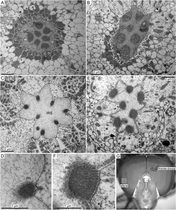
Morphological differences between photoreceptors in the frontal-dorsal and lateral regions of the compound eye. (A,B) Cross-sections at the level of the Semper cells (SC) in the frontal-dorsal (A) and lateral (B) regions of the eye; four Semper cells can be seen in (A); PC, pigment cell; Rh, rhabdomere; RhC, rhabdomere cap. The off-plane section in (B) illustrates the changes at the SC-rhabdomere interface. (C) An ommatidial cross-section in the frontal-dorsal area at the depth of ~50 μm from the surface of the eye; asterisks denote three protruding rhabdomeres; IRS, the intra-rhabdom space; Mt, mitochondrion; RC, retinula cell (photoreceptor). (D) A magnified cross-section of the microvillus array from (C). (E) An ommatidial cross-section in the lateral region at the depth of ~20 μm from the surface of the eye. (F) Magnified cross-section of a microvillus array from (E). (G) Photograph of the hover fly head with designations of the two regions explored in electrophysiological recordings. Insets in (G) are magnified 36-facet plots from the frontal-dorsal and lateral regions as indicated.

The photoreceptor cells contain a specialized light sensitive compartment known as the rhabdomere (Rh), an array of tightly packed microvilli. Rhabdomeres are oriented toward the center of the ommatidium, forming the rhabdom. In flies, individual rhabdomeres are separated by the intra-rhabdom space. Cross-sections of hover fly ommatidia at two levels are presented in Fig. 1A–F. Fig. 1A,B shows the arrangement between the presumed Semper cells and the rhabdomere caps in the distal-most part of the rhabdomere. Still more distally, the Semper cells form an upside-down cup surrounding the rhabdomere caps. The caps connect the tips of the microvillar arrays to the Semper cells, serving as optical waveguide “adapters” (Pask & Barrell, Reference Pask and Barrell1980). Apart from the relatively large caps in the lateral photoreceptor (Fig. 1B), no significant differences can be seen between the two eye regions.
Fig. 1C–F compares representative micrographs of the distal parts of the ommatidia. The differences were salient and consistent: the rhabdomeres in the frontal-dorsal region were notably smaller than in the lateral region. Another difference between the two regions was the absence of a spectral class-specific morphological dimorphism in the frontal-dorsal ommatidia: throughout the retinal depth, there was no clear protrusion of a single rhabdomere toward the center of the ommatidium, a feature of specialized UV or blue-sensitive R7/R8 photoreceptors. In contrast, in sections from the lateral region, there was always one rhabdomere clearly protruding into the intra-rhabdom space (Fig. 1E, asterisk, compare with three protruding rhabdomeres in Fig. 1C).
We also compared the sizes of facets in the two regions by evaluating the areas occupied by the same number of facets from the photograph in Fig. 1G: the 36-facet patch from the frontal-dorsal region was 1.7 times the size of the patch from the lateral region of the eye, consistent with findings of previous studies (see citations in section “Introduction”).
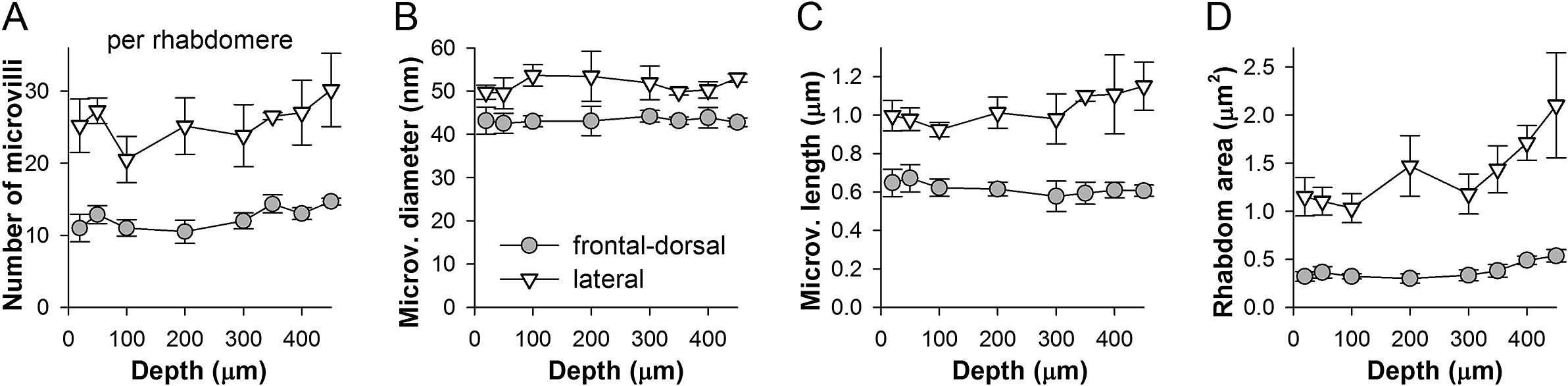
Fig. 2 shows dependencies of the average number, diameter and length of the microvilli, and the transverse rhabdomere areas on the distance from the cornea. The measurements were made by using single, and presumably different ommatidial cross-sections at each depth. Due to variable image quality, the number of microvilli per rhabdomere cross-section was estimated on the basis of two to seven rhabdomeres. The average number of microvilli per rhabdomere was two times higher in the lateral than the frontal-dorsal region (Fig. 1D,F), and tended to increase with the distance from the cornea (Fig. 2A). The average diameter of the microvilli was smaller and they were shorter in the frontal-dorsal than the lateral region (Fig. 2B,C). It should be noted that the microvillus diameter measures are overestimates because we did not take into account the inter-microvillar space. Consequently, the average rhabdomere cross-section areas in the lateral region were about three times larger than in the frontal-dorsal region, with the difference increasing with depth (Fig. 2D).
Quantification of morphological differences between two eye regions. Measurements were made from TEM images of photoreceptors at eight distances from the surface of the eye as indicated, presumably from different ommatidia at each depth. (A) Average number of microvilli per rhabdomere cross-section in the two areas as indicated; depending on the quality of the image, averages were based on counts from 2 to 7 rhabdomeres; here and elsewhere the error bars represent s.d. (B) Average diameters of microvilli were obtained by dividing the widths of the microvillus arrays by the number of microvilli in them; the distance between microvilli was disregarded. (C) Average maximal microvillus lengths; data were obtained by measuring the lengths of the middle microvilli in each array. (D) Changes in the average cross-section areas of the rhabdomere with depth.

Responses to WN and NS: Faster signaling in the love spot
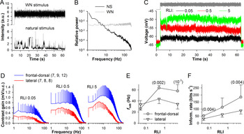
It was previously published that photoreceptors in the frontal region of the male fly eye are characterized by higher corner frequencies than photoreceptors from the same region in females (Hornstein et al., Reference Hornstein, O’Carroll, Anderson and Laughlin2000) or the lateral and ventral parts of the eye in males (Burton et al., Reference Burton, Tatler and Laughlin2001). We performed similar measurements in the hover fly by using a 60 s WN-modulated light intensity time series with a cut off at 250 Hz to determine unbiased corner frequencies and a 60 s NS to explore responses to behaviorally relevant aspects of visual stimuli (Fig. 3A). Fig. 3B shows power spectra of the stimuli.
Stimulation with WN. (A) WN and NS used in experiments shown in Figs. 3 and 4. (B) Power spectra of the stimuli from (A). (C) Three representative voltage responses to the WN stimulus recorded from a frontal-dorsal photoreceptor at three light levels (RLI, relative light intensity). (D) Average contrast gain functions at three intensities; gain was measured in millivolts per unit of contrast (u.c.); in the legend, numbers in the parentheses denote the number of data points in each average trace, respectively. (E,F) Dependencies of corner frequencies (E) and information rates (F) on the stimulus intensity; corner frequencies were obtained by fitting individual gain traces with a Hill equation in the range from 5 to 200 Hz; the numbers of values in each average were the same as in (D); unpaired t-test with unequal variances was used for statistical comparisons, with numbers in parentheses indicating the P-values.

Fig. 3C–F presents the results of WN experiments. Voltage responses of a photoreceptor from the frontal-dorsal region recorded at three intensities are shown in Fig. 3C. Averaged contrast gain functions are shown in Fig. 3D. The low-pass corner frequencies (f 3dB) were determined by fitting the contrast gain functions with Hill equations in the range from 5 to 200 Hz. On average, the highest f 3dB values were found at relative light intensity (RLI) 0.5: 64 ± 4 Hz in the frontal-dorsal versus 44 ± 8 Hz in the lateral region (Fig. 3E). Although, the maximal contrast gain appeared to be higher in the frontal-dorsal than the lateral photoreceptors, the differences were not statistically significant due to high variability. Average information rates were significantly higher in the frontal-dorsal than lateral photoreceptors (Fig. 3F).
The observed decrease in f 3dB at the brightest WN intensity can only be caused by the broadening of responses to changes in light intensity. Such development opposes the general adaptation-caused decrease in light response duration (Howard et al., Reference Howard, Dubs and Payne1984). While the mechanisms of such broadening in bright light are not exactly known, a plausible mechanism is the light intensity dependent activity of the depolarizing sodium–calcium exchanger (Chu et al., Reference Chu, Postma and Hardie2013) (also see Fig. 8A, bottom).
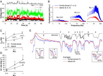
The differences in the corner frequency between the experimental groups indicated that frontal-dorsal photoreceptors can respond more robustly to higher-frequency stimuli than lateral photoreceptors, consistently with their main function of detecting fast-flying small dark objects against bright background. In M. domestica, transient dimming can generate hyperpolarizations of variable kinetics and duration depending on the angular size and tangential velocity of the moving object (Burton & Laughlin, Reference Burton and Laughlin2003). We therefore investigated responses of hover fly photoreceptors to different aspects of visual stimuli by using a contrast-rich NS (Figs. 3A,B and 4). Typical responses of a frontal-dorsal photoreceptor are shown in Fig. 4A. Average gain functions are shown in Fig. 4B. Average low-pass corner frequencies and information rates are shown in Fig. 4C,D. Average f 3dB at RLI 1 were identical to those found in WN recordings at RLI 0.5: 62 ± 6 Hz in the frontal-dorsal and 43 ± 6 Hz in the lateral photoreceptors (Fig. 4C). The maximal gain values were not statistically significantly different. The differences in average information rates (Fig. 4D) were consistent with the WN results (Fig. 3F).
Stimulation with NS. (A) Three voltage responses of a frontal-dorsal photoreceptor to the NS stimulus. (B) Average contrast gain functions at three intensities. (C,D) Dependencies of corner frequencies (C) and information rates (D) on the stimulus intensity; the numbers of values in each average were as indicated in B; unpaired t-test with unequal variances was used for statistical comparisons. (E) Comparison of averaged responses at RLI 1 for the 1.6 s segment of elevated stimulation background (asterisk in A); numbers denote areas of interest (see section “Results”); response amplitudes were aligned before #2; normalized stimulus and responses corresponding to events #2, 4 and 8 are shown separately in insets.

It can be shown by using the average contrast gain functions (Fig. 4B) that, for instance, at RLI 1 at 100 Hz the contrast gain is 5.6-fold higher in the frontal-dorsal than the lateral photoreceptors. If the curves were normalized to isolate the contribution of the bandwidth, the difference at 100 Hz would decrease to 2.9-fold. Fig. 4E illustrates consequences of these differences for the recoding of light contrasts into graded voltages. The figure shows average responses to a particularly negative contrast-rich part of the stimulus at the brightest light intensity (Fig. 4A, asterisk). In addition to the increased gain of the frontal-dorsal response, there was a salient difference in the character of transient signal processing. For instance, the prolonged events #2, 5 and, to a lesser extent, events #1, 7 and 9, were transferred with a similar resolution of fine details by the frontal-dorsal and lateral photoreceptors. However, the majority of small and rapid transients of #3, the isolated events #4 and #6, and the first transient of #8 barely registered in the response of the lateral photoreceptors. Comparison of the normalized events #2, 4 and 8 shown in the insets suggests that the differences in the graded signals are probably caused by the relatively slow kinetics of responses of the lateral photoreceptors. Overall, it appeared that the faster and more transient was the change in light intensity, the better it was recoded by the frontal-dorsal photoreceptors, regardless of the event polarity.
Membrane response properties
The differences in signal processing between the frontal-dorsal and lateral photoreceptors could be due to: (1) the differences in the properties of the light-insensitive membrane, (2) basal phototransduction, or/and (3) light adaptation.
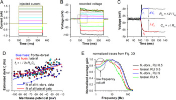
To study membrane resistance and capacitance in the dark, we recorded electrical responses to step current injections (Fig. 5A,B). Membrane capacitance and membrane resistance were estimated as shown in Fig. 5C. Changes in the character of voltage responses with depolarization indicated the presence of rapidly activating sustained conductances similar to those found in other fast diurnal flies (Laughlin & Weckström, Reference Laughlin and Weckström1993).
Filtering by the light-insensitive membrane. (A–C) Measurement of membrane resistance (Rm), time constant (τ), and capacitance (Cm) in the dark. A series of injected current pulses (A) elicited voltage responses (B), from which τ, Rm and Cm were measured (C); τ was obtained by fitting the onset of a voltage response with a single-exponential equation (red or blue traces), and Rm and Cm according to the equations; I inj, a current injected to evoke the voltage responses. To improve the estimates, Rm and Cm were determined by using the first depolarizing and hyperpolarizing responses around the resting potential and then averaging the obtained values. (D) Dependencies of corner frequencies on membrane potentials for 12 photoreceptors from the frontal-dorsal (bluish hues) and 9 photoreceptors from the lateral (reddish hues) eye regions; each photoreceptor is denoted by a distinct set of uniform symbols, with one set (blue circles) connected with thin lines for illustration; corner frequencies were obtained as shown in the equation; the Rm values were determined from the current-clamp recordings as averages between the consecutive voltage amplitudes. To discover general trends, all values from the two regions were pooled together and fitted by single-exponential equations. (E) Normalized contrast gain functions from WN experiments from Fig. 3D.

Resistance at resting potential was measured as the average of amplitudes of two settled voltage responses, to the hyperpolarizing (−0.25 nA) and depolarizing (0.25 nA) current pulses. Membrane capacitance was determined from the time constants of the voltage response onsets (τ 1 and τ 2, Fig. 5C). No significant differences were found between the frontal-dorsal and lateral photoreceptors: correspondingly, the average resistance was 45 ± 21 (n = 20) versus 50 ± 14 MΩ (n = 11), the average capacitance 41 ± 21 versus 33 ± 13 pF, and the average membrane time constant at resting potential 1.52 ± 0.46 versus 1.46 ± 0.32 ms. In turn, these time constants corresponded to the average corner frequencies of 113 ± 28 and 114 ± 30 Hz, respectively. These values are substantially higher than the corner frequencies obtained in the WN and NS experiments (Figs. 3E and 4C), indicating that low-pass filtering by the light-insensitive membrane is permissive.
Because voltage-gated conductances expressed in the soma can nonlinearly modify light responses (Weckstrom et al., Reference Weckstrom, Hardie and Laughlin1991; Laughlin & Weckström, Reference Laughlin and Weckström1993), it was necessary to investigate possible differences in the dynamic membrane impedance between the two regions. The conventional approach of determining impedance involves injections of WN-modulated current (Hornstein et al., Reference Hornstein, O’Carroll, Anderson and Laughlin2000). However, we could not use this method because depolarizing current pulses often caused artifacts (compare voltage responses to the three most depolarizing current pulses in Fig. 5B). While these could be recognized in responses to constant current steps, no reliable criteria could be set for artifact recognition and elimination in voltage responses to irregular noise-modulated current injections.
Therefore, we first investigated low-pass corner frequencies of membrane in the dark over a range of membrane potentials (Fig. 5D), and then examined the so-called low-frequency roll-offs caused by high-pass filtering by fast-activating delayed rectifier K+ channels and usually manifesting in the form of hyperpolarization after a brief light response (Fig. 5E).
We estimated voltage-dependencies of the membrane corner frequencies (fc) by using Cm obtained at rest as described above and the varying membrane resistances from the current-clamp recordings (equation in Fig. 5D). Because of high variability in the data, we pooled all voltage-dependencies of corner frequencies together and fitted them with single-exponential equations (Fig. 5D). The corner frequencies increased with voltage as expected, with their average estimates reaching ~150 Hz at −40 mV and ~200 Hz at −30 mV. The trends were nearly the same for both experimental groups.
Fig. 5E shows average contrast gain functions from experiments described in Fig. 3. A clear low-frequency roll-off emerged at the highest light intensity, RLI 5 (Fig. 5E). In both experimental groups, the contrast gain at 2 Hz was on average 75% of its peak value.
These observations suggest that the differences in signal processing between frontal-dorsal and lateral photoreceptors discovered in WN and NS experiments (Figs. 3 and 4) cannot be explained by dissimilarities in electrophysiological properties of the light-insensitive membrane.
Elementary light responses
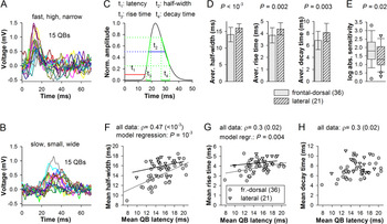
Next, we investigated the elementary responses, voltage QBs. To evoke QBs, dark-adapted photoreceptors were stimulated with 1 ms low-intensity flashes at a frequency of ≤2 Hz. Stimulus intensity was adjusted to evoke single bumps with a probability in the range from 0.1 to 0.5. Voltage bumps were small and irregular, and appeared against a noisy background, with noise fluctuations often exceeding bump-like transients, which is typical for photoreceptors of diurnal fliers (Frolov & Ignatova, Reference Frolov and Ignatova2020b). QBs suitable for analysis were obtained from 36 photoreceptors in the frontal-dorsal and 21 photoreceptors in the lateral eye region. QBs were analyzed in the following fashion. Flash-triggered QB-like events (Fig. 6A,B) were individually fitted with a voltage-dependent relaxation equation:
 $$ f(V)=\frac{1}{a_0{e}^{\frac{V}{\alpha }}+{b}_0{e}^{\frac{V}{\beta }}}+C. $$
Elementary responses. (A,B) Examples of voltage bumps recorded from two photoreceptors illustrate variability between photoreceptors; in these recordings QBs were elicited with a probability of <0.3; stimulus is given at 0 ms. (C) Definition of QB parameters. (D) Comparison of group-average half-widths, 25–75% rise and decay times; unpaired t-test was used for statistical comparisons. (E) Box plot compares the absolute sensitivities; values are reciprocals of light intensities used to evoke QBs; horizontal lines within the boxes are medians; bottom and top of boxes, lower 25% and upper 75% quantiles; whiskers, the variability outside the upper and lower quartiles; symbols, the outliers; Mann–Whitney U test was used for statistical analysis. (F–H) Dependencies of mean half-widths (F), 25–75% rise (G), and decay (H) times on mean latencies; Spearman’s rank order correlation coefficients ρ were calculated for all data pooled together; in (F,G) data groups were also fitted separately with linear equations to emphasize different trends; statistical comparison was performed by fitting to a regression model.

The fitting waveform was used to estimate individual QB latency (at 10% amplitude), half-width, 25–75% rise and decay times (Fig. 6C). Fig. 6A,B shows that hover fly QBs were characterized by significant variability in mean QB parameters between photoreceptors. In the following presentation of QB results we use the term “mean” to describe single photoreceptor data, that is, average of all individual QB values from a photoreceptor. The term “average” refers to the group averages, that is, average of all mean data, with the accompanying s.d. describing variability between the mean values.
We found statistically significant group differences between several properties of QBs. Average QB latency, which was determined as the time interval between the onset of flash and the time QB amplitude reached 10% of its maximum, were similar: 14.9 ± 2.9 ms in the frontal-dorsal and 15.7 ± 2.0 ms in the lateral photoreceptors. Average QB amplitudes were also similar: 0.83 ± 0.18 mV in the frontal-dorsal and 0.80 ± 0.14 mV in the lateral photoreceptors. However, frontal-dorsal photoreceptors were on average narrower, had faster onsets and decays than QBs in the lateral photoreceptors (Fig. 6D). Correspondingly, the average QB half-widths were 14.0 ± 2.2 versus 16.4 ± 1.5 ms (P < 10−3); the 25–75% rise times 3.8 ± 0.6 versus 4.6 ± 0.6 ms (P = 0.002); and the 75–25% decay times 6.8 ± 1.5 versus 8.2 ± 1.4 ms (P = 0.003).
We have also compared stimulus intensities at which the QBs were evoked. Their reciprocals provide estimates of absolute sensitivity. There was a large variability between photoreceptors (Fig. 6E). Analysis indicated that median absolute sensitivity of the frontal-dorsal photoreceptors was three times higher than that of the lateral photoreceptors (Fig. 6E).
We have previously established that mean activation-related parameters of QBs in the blow fly P. terraenovae and cockroach P. americana depend on the mean latency: as the latter decreased, both the mean QB half-width and mean rise time decreased, whereas mean QB amplitude increases (Frolov & Ignatova, Reference Frolov and Ignatova2020a). Therefore, it was important to examine if a similar pattern existed in the hover fly. Fig. 6F shows that mean QB half-width increased with mean latency (ρ = 0.47). Similarly, there was a weak positive correlation between mean latencies and rise times (Fig. 6G), and a weak positive correlation between mean latencies and decay times (Fig. 6H). Consistently with the previous study, mean QB amplitudes tended to decrease with increasing latencies, but the correlation was not statistically significant.
The data distributions in Fig. 6F,G overlapped only partly, indicating that variation in the cascade speed cannot fully explain the variabilities in mean half-widths and rise times. The differences were assessed in a linear regression model. The discrepancies between latency/half-width and latency/rise-time data groups were statistically significant. Overall, these results suggest that the rate of light-activated channel opening after crossing the latency measurement threshold and also the rate of inactivation were different in the two regions, resulting in significantly different average QB half-widths.
It should be noted that although resting potential in these experiments varied from −42 to −82 mV, with the average of −61.5 ± 8.9 mV for the frontal-dorsal and −63.6 ± 10.2 mV for the lateral photoreceptors, the studied QB parameters did not depend on it, with the exception of amplitude, which decreased steadily as resting potential depolarized.
Light adaptation
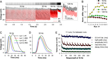
So far, we have found differences in the properties of QBs recorded from dark-adapted photoreceptors, including increased QB half-width in the lateral photoreceptors (Fig. 6D,F). These findings were consistent with the differences in signal processing discovered in WN and NS experiments (Figs. 3 and 4). However, light responses can undergo dramatic changes during light adaptation (Howard et al., Reference Howard, Dubs and Payne1984; Juusola & Hardie, Reference Juusola and Hardie2001) possibly superseding the modest differences in the properties of QBs. It was therefore necessary to investigate the development and effects of light adaptation. A conventional approach to study light adaptation involves sustained stimulation to drive the cell into a certain adaptation state and then adding brief flashes to elicit small impulse responses on top of sustained depolarization. However, such protocol would not allow investigating the development of light adaptation, which in flies occurs at a subsecond scale. We used an incrementing flash frequency stimulus consisting of four 30-pulse series of 1 ms flashes applied at 16, 32, 64, and 128 Hz. To explore the range of changes associated with light adaptation, stimulus intensity was modified with neutral density filters.
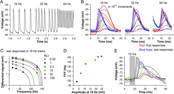
Fig. 7 illustrates development of light adaptation in one photoreceptor during repetitive stimulation. Fig. 7A shows two response trains evoked by the same stimulus but separated by seven runs, with 5 s inter-run dark intervals. Although the signal amplitude in the low-frequency series remained virtually the same, the signal at 128 Hz from run #9 was clearly higher than that from run #1 (Fig. 7A, inset). When the differential signals (determined as the difference between the adjacent peaks and lows) were normalized by dividing with the amplitude of the differential signal from the first run, it emerged that light adaptation caused a gradual saturating increase at 128 Hz and to a lesser extent at 64 Hz (Fig. 7B). Comparison of the first and last voltage responses in the 16 and 32 Hz trains from runs #1 and #9 elucidated the observed mechanism of light adaptation (Fig. 7C,D). The first response of run #1 was characterized by a twofold higher latency and half-width than the last response of run #9. The differences were less pronounced in the 32 Hz train (Fig. 7D), suggesting that the effects of light adaptation were largely settled by the end of the 16 Hz trains.
Changes during light adaptation. (A) A frontal-dorsal photoreceptor was stimulated 11 times at the same intensity by the incrementing flash frequency stimulus (top) consisting of 120 1-ms pulses given at four frequencies, 16, 32, 64, and 128 Hz; 5 s intervals separated the runs. Two response trains (runs #1 and #9) characterized by the largest differences in the differential signal at 128 Hz (inset) are superimposed; (B) Comparison of normalized differential signals shows strong augmentation at 128 Hz; differential signals were obtained by subtracting several minima of membrane potential from the neighboring peaks at the end of each frequency domain and averaging the values. (C,D) Superposition of first and last impulse responses from the 16 (C) and 32 (D) Hz trains during runs #1 and 9; stimulus is given at 0 ms. (E) Plots of response latency (time the amplitude reached 0.5 mV during the onset phase), half-width, amplitude, 25–75% rise and decay times at 16 Hz for the entire experiment; the inter-run intervals are not shown.

Fig. 7E shows changes in response amplitudes, latencies, half-widths, 25–75% rise and 75–25% decay times in 16 Hz trains during the entire experiment. Here, the response latency was defined as an interval between the stimulus and the time when response voltage increased by 0.5 mV during the onset. Dynamics of changes in latency, rise and decay times, and also in half-width during the first run were quite similar, whereas amplitude decreased very little. However, the half-width recovered substantially during the 5 s inter-run periods in the dark, whereas latency, and 25–75% rise and decay times did not. This indicates that half-width is not fully determined by the changes in light response kinetics. Moreover, this lack of time course correlations suggest distinct mechanisms for changes in different response parameters (see section “Discussion”).
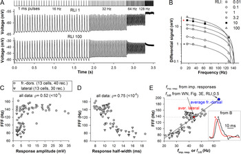
Fig. 8 demonstrates how response properties can change with stimulus intensity. Fig. 8A shows recordings from a frontal-dorsal photoreceptor at two intensities. The responses started merging at 32 Hz, and only small differential signals remained at 128 Hz. Notably, response amplitudes decreased little as stimulation proceeded even at the brightest level (Fig. 8A, low trace). Responses at RLI 100 in the 16 Hz train were characterized, exclusively in this experiment, by distinct after-depolarizations probably caused by activation of the sodium–calcium exchanger.
Limits of frequency resolution. (A) Examples of responses of a frontal-dorsal photoreceptor to the incrementing flash frequency stimulus at two intensities (RLI of 1 and 100). (B) Differential signals from six recordings from the same photoreceptor were plotted against train frequency and fitted with linear equations. (C,D) Dependencies of flicker fusion frequency (FFF) values on the amplitudes (C) or half-widths (D) of impulse responses at the end of the corresponding 16 Hz trains. (E) Correlations between FFF and corner frequencies of amplitude spectra of impulse responses (f imp. resp.). To obtain f imp. resp., the impulse response was first fitted with a lognormal equation at 100 kHz sampling rate; the amplitude spectrum was then obtained as a square root of the power spectrum of the fitting curve. By using the apparent linear dependence of FFF on f imp. resp., we estimated FFF values, which could be associated with the fully light-adapted corner frequencies f 3dB from the WN experiments (Fig. 3). Inset to the right: normalized impulse responses (last responses in 16 Hz trains of the last runs) from trains recorded at different intensities from (B; asterisks).

When differential signals obtained from six recordings in the same photoreceptor were plotted against frequency and fitted with linear equations, clear linear relationships emerged for all recordings (Fig. 8B), except for the highest intensity one (RLI 100) characterized by adaptive decreases of amplitudes that at 32 and 64 Hz (Fig. 8A). By extending the linear fitting lines to the x-axis, we obtained extrapolations of the absolute limits of signal processing at the current operational state, the analogues of the flicker fusion frequency (FFF). (Note, that if the differential signal was absent at 128 Hz, the zero was not plotted to avoid biasing.)
To investigate which properties of impulse responses influence the FFFs the strongest, we plotted them against the amplitudes (Fig. 8C) or half-widths (Fig. 8D) of the last impulse responses in the corresponding 16 Hz trains. While the amplitudes appeared to be relatively poor predictors, a very strong negative correlation was found between the FFF and half-width values.
Because under the same light adaptation conditions, the amplitude spectrum of an impulse response to an instantaneous stimulus is equivalent to the WN transfer function gain, it was possible to correspond the FFF values through the corner frequencies of amplitude spectra of our flash responses (f imp. resp.) to the corner frequencies of gain functions from the WN experiments (Fig. 8E). We obtained f imp. resp. for all last responses in the 16 Hz trains of the last runs of flash stimulation experiments (see examples of responses and the associated amplitude spectra in Fig. 11E,F). Note, that the normalized responses characterized by a ~20-fold difference in amplitude from Fig. 8E, inset, have similar shapes. These f imp. resp. can be considered as situational corner frequencies because they describe momentary adaptation states dependent on stimulation intensity and its immediate history. A linear dependence emerged when we plotted FFF against the f imp. resp. values (Fig. 8E).
To estimate the FFF values associated with the fully light-adapted photoreceptors from the WN experiments, we placed average f 3dB values from Fig. 3E (at RLI 0.5) on the line fitting all data in Fig. 8E, and then dropped projections on the y-axis. The predicted average FFF values were 195 Hz for the frontal-dorsal and 138 Hz for the lateral photoreceptors. The lateral photoreceptors stimulated with bright flashes reached the state of adaptation similar to that during WN stimulation, whereas the frontal-dorsal photoreceptors did not.
Different adaptation states
The data points from two experimental groups overlapped fully in Fig. 8C–E, indicating similar mechanisms of light adaptation between the two parts of the eye. However, these results could not explain why frontal-dorsal photoreceptors were characterized by much higher corner frequencies than the lateral photoreceptors in the WN and NS experiments (Figs. 3E and 4C). We hypothesized that frontal-dorsal photoreceptors can reach a more advanced adaptation state during continuous stimulation than during pulsed stimulation. Indeed, we have demonstrated that the frontal-dorsal photoreceptors were characterized by about threefold higher absolute sensitivity than the lateral photoreceptors (Fig. 6E), suggesting that the same stimulus could excite the former stronger than the latter.
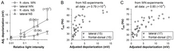
We compared how WN and NS stimulation depolarized photoreceptors in the two regions (Fig. 9A). Dependencies of depolarization on light intensity were characterized by the same trends for WN and NS experiments. In bright light, the frontal-dorsal photoreceptors were characterized by significantly stronger sustained depolarizations than lateral photoreceptors. Because the force driving the light-induced current (LIC) and thus the magnitude of depolarization measured as a difference between the resting and sustained response potential depends on the membrane potential, the values recorded from dissimilar resting potentials were adjusted to the common level of −60 mV, assuming the Nernst potential for LIC of +10 mV (this adjustment was conservative because we did not take into the account the voltage-dependence of membrane resistance, Fig. 5D).
Photoreceptor depolarization and corner frequency. (A) Dependencies of average sustained depolarization on stimulus intensity during responses to WN and NS stimuli; the numbers of values at each light level were as in Figs. 3D and 4B; values were obtained by averaging the entire response after de-trending by subtracting the resting potential before and after the response; to account for the differences in depolarization due to different resting potentials and thus LIC driving forces, all values were recalculated for −60 mV by assuming LIC reversal potential of +10 mV. Values in parentheses are P-values for the respective means, unpaired t-test was used. (B,C) Dependencies of f 3dB values of individual responses on the adjusted depolarization values for the NS (B) and WN (C) experiments.

While the differences in sustained depolarization between the frontal-dorsal and lateral photoreceptors were unambiguous, it was necessary to prove that stronger depolarization is really associated with stronger light adaptation and vice versa. We therefore plotted corner frequencies of contrast gain functions of individual recordings against the corresponding depolarizations (Fig. 9B,C). While all data from NS experiments were used in Fig. 9B, we excluded some WN data, which were obtained at RLI 5 and characterized by a decrease in f 3dB after its maximum at RLI 0.5 (Fig. 3E, see discussion of the “saturation” in text). As a result, strong positive correlations have emerged supporting the hypothesis that the superior f 3dB values of the frontal-dorsal photoreceptors (Figs. 3E and 4C) are due to the comparatively advanced adaptation state caused by increased excitation.
Spike-like responses in the axon augment transfer of higher frequencies
Some recordings associated with deeper than usual positions of the electrode in the tissue demonstrated spike-like events (fast depolarizing transient) during the onset of impulse responses, suggesting that the electrode penetrated the cell in or near the axon (Weckström et al., Reference Weckström, Juusola and Laughlin1992). Fig. 10A shows spike-like responses on top of impulse responses recorded from a photoreceptor in the lateral part of the eye. Because the shape of impulse responses changed during the trains, the visibility of spikes gradually decreased. We compared the shapes of first and last impulse responses in 16, 32, and 64 Hz trains at six stimulation intensities (Fig. 10B). There was no indication of spikes in the response pairs at three lowest intensities but they appeared in the responses exceeding 10 mV. Fig. 10C shows dependencies of the differential signals at different light intensities on frequency and Fig. 10D dependence of FFF on the response amplitude at 16 Hz.
Spikes in the lateral eye region. (A) A part of a response train with spikes visible at the peaks. (B) Spikes and light adaptation-related shortening of impulse responses at different frequencies from (A). (C) Six differential signals from the same cell fitted with linear equations from the dimmest (red triangles) to the brightest (pink hexagons) light intensity. (D) Dependence of the FFF on the impulse response amplitude at 16 Hz. (E) Spikes strongly modify prolonged responses to 10 ms stimuli of increasing intensity; light intensity was increased in twofold increments.

The effect of spikes on the light response can be more apparent if a photoreceptor is stimulated with prolonged flashes. Fig. 10E shows induction of large spikes by 10 ms pulses of incrementing intensity in a dark-adapted photoreceptor. In this example, spikes strongly accelerated the onset and increased the amplitude of light responses.
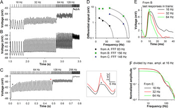
Fig. 11 demonstrates how spikes can selectively and nontrivially amplify responses to higher-frequency stimulation. Fig. 11A,B shows responses of a frontal-dorsal photoreceptor at two intensities. In Fig. 11A, the responses were quite small and without spikes. During higher-intensity stimulation in Fig. 11B, spikes emerged and the differential signal at 64 Hz clearly exceeded that at 16 and 32 Hz. Consequently, the FFF increased from 83 Hz in Fig. 11A to 156 Hz in Fig. 11B.
Spikes expand the signaling range in the frontal-dorsal region. (A,B) Responses of a photoreceptor at two light intensities. (C) Response of the same cell to a higher-frequency stimulus train (64–128–256 Hz) at a fourfold lower light intensity than in (B); the trace is average of 20 runs separated by 6 s intervals in the dark; inset to the right: superposition of the 2nd and 29th responses in the 64 Hz train (asterisks). (D) Three differential signals from panels A–C fitted with linear equations; FFF values are in the legend. (E) Last responses from 16, 32, and 64 Hz response trains from (B); stimulus is given at 0 ms. (F) Amplitude spectra of traces from E; spectra were divided by the maximum value of the 16 Hz trace spectrum.

An unusual example of spike development is shown in Fig. 11C. The same photoreceptor was stimulated 20 times by high-frequency trains, starting from 64 Hz, with 6 s intervals in the dark between the runs. Unexpectedly, the spikes increased gradually as the 64 Hz train proceeded. Inset shows a very small spike on the front edge of the second response in the train. However, by the end of the train the spike increased dramatically. It is not known whether this phenomenon is related to the slight elevation of membrane potential in-between the pulses, or to a use-dependent facilitation of channels mediating the spikes.
Fig. 11D summarizes the effect of spikes on FFF in this experiment. Fig. 11E illustrates changes in the last responses from 16, 32, and 64 Hz trains in Fig. 11B. Consistently with the apparently strongest effect on the green trace, the amplitude spectra of the responses from Fig. 11E demonstrate that the spike-induced enhancement at around 150 Hz was the strongest for the 64 Hz stimulation train, reaching one fifth of its maximal amplitude (Fig. 11F).
Discussion
We performed a morphological and electrophysiological study of photoreceptors in the hover fly, investigating differences between the frontal-dorsal and lateral regions of the compound eye. We found: (1) prominent morphological differences between the two regions, (2) differences in signal processing in bright light, to the advantage of the frontal-dorsal photoreceptors, (3) differences in properties of QBs, (4) demonstrated that superior performance of the frontal-dorsal photoreceptors was due to a comparatively advanced state of light adaptation caused by their increased sensitivity, and (5) showed that spikes recorded in the proximal part of the photoreceptor or the axon can strongly amplify voltage responses in the higher-frequency range. Overall, our results support the notion that the frontal-dorsal region in male fly is specialized for high acuity, high temporal resolution vision. Below we discuss our main findings.
Morphological differences
We investigated the morphology of the ommatidia down to ~450 μm depth from the surface of the eye. Fig. 2 indicates that the number of microvilli per rhabdomere cross-section and their lengths (in the lateral region) increased gradually with depth. Consequently, the ratio of the average lateral to frontal-dorsal rhabdomere cross-section areas increased from about three in the distal to about four in the proximal part of the ommatidium.
The rhabdomere diameters in the frontal-dorsal region were very small, ~0.6 μm, the smallest sizes for the green-sensitive photoreceptors reported to date for an insect. For comparison, in the frontal acute zone R1-6 rhabdom diameter is ~0.8 μm in the house fly (Franceschini et al., Reference Franceschini, Hardie, Ribi and Kirschfeld1981), ~1 μm in the hunter fly (Gonzalez-Bellido et al., Reference Gonzalez-Bellido, Wardill and Juusola2011), ~0.9 μm in robber fly (Wardill et al., Reference Wardill, Fabian, Pettigrew, Stavenga, Nordstrom and Gonzalez-Bellido2017), and even in the smallest of insects it exceeds 1.4 μm (Fischer et al., Reference Fischer, Muller and Meyer-Rochow2011; Fischer et al., Reference Fischer, Meyer-Rochow and Muller2012). The diameter of the rhabdomere as a light guide cannot be reduced indefinitely without compromising the ability to conduct light. Thus green-sensitive photoreceptors rarely have rhabdomere diameter <1 μm, but it is usually smaller for blue- and UV-sensitive photoreceptors (Snyder & Miller, Reference Snyder and Miller1972; Horridge et al., Reference Horridge, Mimura and Hardie1976; Stavenga, Reference Stavenga2004a,Reference Stavenga b).
Light rays impinging on the tip of an ideal cylindrical waveguide with the refractive index (n 2) exceeding that outside (n 1) can propagate within the fiber with relatively little losses. When the impinging angle is smaller than the critical angle dependent on the ratio of the refractive indices, light wavelength (λ) and fiber diameter (d) (see section 3.2 in Snyder, Reference Snyder, Snyder and Menzel1975), and the ray is meridional, it can undergo total internal reflection and become trapped inside or bound. When the angle is greater, the rays undergo only partial internal reflection, losing energy each time, hence their leaky character. Propagation of both bound and leaky rays is described by solutions of an eigenvalue equation (Snyder, Reference Snyder, Snyder and Menzel1975) and occurs in the form of discrete modes, with the bound modes representing stable and leaky modes attenuating light distributions along the waveguide. The amount of light power transferred by a mode is generally reciprocal to its order (Snyder, Reference Snyder, Snyder and Menzel1975). The number of modes that can propagate in a fiber is determined by V-number:
 $$ V=\frac{\pi d}{\lambda}\sqrt{n_1^2-{n}_2^2.} $$
Modal propagation of light was reported in fly rhabdomeres (Van Hateren, Reference Van Hateren1984). Here we found an extraordinarily small rhabdomere diameters (see Figs. 1C,D and 2A–C) in the frontal-dorsal region of the hover fly eye. By using the refractive indices previously estimated for fly rhabdomeres (n 1 = 1.339 and n 2 = 1.364) (Beersma et al., Reference Beersma, Hoenders, Huiser and Van1982), we calculated V-numbers for two idealized waveguides with diameters of 600 and 1000 nm corresponding to the average rhabdomere cross-sections in the frontal-dorsal and lateral regions. V for light of 500 nm was 0.98, indicating that only 17% of light power contained in the first-order bound mode η 11 (nomenclature by Snyder, Reference Snyder, Snyder and Menzel1975) is trapped inside the waveguide of 600 nm in diameter, with the rest propagating outside. Twice as much light power can be trapped inside when violet light (λ = 400 nm) propagates instead. The waveguide with d of 1000 nm, while substantially more permissive, at 500 nm still allowed propagation of only the first mode.
Thus the rhabdomeres in the frontal-dorsal region can conduct only a small portion of green wavelengths in the bound modes, and this would shift the effective sensitivity range toward short wavelengths, arguably facilitating detection of small dark objects moving against the blue sky and also preventing photoreceptor overstimulation. The narrowing of the rhabdomere is also associated with the narrowing of the acceptance angle, which, together with other morphological adaptations in the frontal-dorsal eye region of V. pellucens—the increased facet diameter and decreased interommatidial angle (0.7–1.1° vs. 1.4–1.5° in the lateral parts of the retina)—would improve visual acuity, facilitating detection, tracking, and capture of flying females (Kirschfeld, Reference Kirschfeld, Zettler and Weiler1976; Horridge & Duelli, Reference Horridge and Duelli1979; Rossel, Reference Rossel1979; Stavenga, Reference Stavenga2004a; Warrant, Reference Warrant2016).
These considerations suggest that dark-adapted frontal-dorsal photoreceptors should be less sensitive to green light than the lateral photoreceptors. However, this is inconsistent with our electrophysiological finding of a threefold higher sensitivity of the former, which, as we showed, was essential for the development of a relatively deep adaptation state facilitating transfer of high frequencies. Although the increased sensitivity could be partly attributed to the increased facet diameters, other unidentified mechanisms might also be involved.
Differences in signal processing
We used several approaches to compare photoreceptor performance and determine the mechanisms responsible for the differences we found. Apart from the conventional WN stimulus (Fig. 3) allowing proper evaluation of transfer function, we used a NS (Fig. 4). Comparison of frontal-dorsal and lateral photoreceptors revealed prominent differences in responses to fine transient changes in light intensity (Fig. 4E). Our results were consistent with another electrophysiological study directly comparing functioning of photoreceptors between the frontal, lateral and posterior regions of the male blowfly Calliphora vicina eye (Burton et al., Reference Burton, Tatler and Laughlin2001). In still another study comparing frontal photoreceptors of male and female M. domestica, authors found significant advantages of male photoreceptors, which were characterized by comparatively high bandwidths of transfer function in WN stimulation experiments (Hornstein et al., Reference Hornstein, O’Carroll, Anderson and Laughlin2000).
Burton and Laughlin (Reference Burton and Laughlin2003) found that nonlinear mechanisms play major roles in boosting the contrast gain and reducing the duration of the hyperpolarizing responses of love spot photoreceptors to a dark moving target. The first nonlinearity manifests in the increasing contrast gain as the hyperpolarizing response increases due to hyperbolic relationship between response and intensity. The second one is amplification and sharpening of depolarizing responses by voltage-activated Ca2+ or Na+ channels.
In M. domestica, membrane impedance of male photoreceptors exhibited a relatively strong roll-off in the low-frequency region, which could additionally contribute to acceleration of impulse response decay (Hornstein et al., Reference Hornstein, O’Carroll, Anderson and Laughlin2000). While we did not explore comprehensively the properties of light-insensitive membrane in V. pellucens, we found no differences in the filtering by the light-insensitive membrane between the regions. The estimated dependencies of membrane corner frequency on membrane potential were nearly identical (Fig. 5D), substantially exceeding the corner frequencies of contrast gain (Figs. 3E and 4C). When we compared the low-frequency roll-offs of the contrast gain functions (Fig. 5E) probably caused by high-pass filtering mediated by the rapidly activating delayed rectifier K+ channels (Heras et al., Reference Heras, Laughlin and Niven2016), we also found no significant differences.
Analysis of QBs confirmed our previous findings made in the cockroach P. americana and blow fly P. terraenovae on the dependence of QB activation-related parameters on the latency of phototransduction (Frolov & Ignatova, Reference Frolov and Ignatova2020a). We also found that QBs evoked in the lateral photoreceptors were wider, and had slower onset and termination kinetics than QBs recorded from the frontal-dorsal photoreceptors. We propose that these differences might be caused by dissimilar volumes of microvilli. We estimated average microvillar cytosol volumes on the basis on the morphological measurements (Fig. 2B,C), taking into account the combined membrane thickness, the inter-microvillar space, and the volume occupied by the central actin filament. The average microvillus in the frontal-dorsal region was by ~60% smaller in the volume than in the lateral region. Such differences could result in substantially faster accumulation of calcium in the smaller microvillus, speeding up both the onset and termination of the QB. The QB onset depends on the Ca2+-dependent positive feedback, so that Ca2+ entering the microvillus via the first opened TRP channels facilitates opening of other channels (Nikolic et al., Reference Nikolic, Loizu, Degenaar and Toumazou2010; Hardie, Reference Hardie2012; Hardie & Juusola, Reference Hardie and Juusola2015). This is consistent with insignificant differences in average latencies between the frontal-dorsal and lateral photoreceptors, which we determined at the low amplitude threshold of 10%, but significant differences in the 25-75% QB rise and decay times (Fig. 6D). QB termination is mainly regulated by calmodulin and PKC, which are activated by the influx of Ca2+ during the QB (Nikolic et al., Reference Nikolic, Loizu, Degenaar and Toumazou2010; Hardie & Juusola, Reference Hardie and Juusola2015). Although the levels of expression of calmodulin and PKC could also be dissimilar in the two eye regions, this could not be tested.
Interestingly, the differences in the microvillus dimensions between the two regions of the hover fly eye were very similar to those in the housefly M. domestica, where photoreceptors in the love spot have thinner and shorter microvilli than in the peripheral retina: 40 and 610 nm versus 60 and 1000–2000 nm, respectively (Boschek, Reference Boschek1971; Hardie et al., Reference Hardie, Franceschini, Ribi and Kirschfeld1981).
Crucially for this study, we found in QB experiments that frontal-dorsal photoreceptors were more sensitive than their lateral counterparts (Fig. 6E). As we have shown in WN and NS experiments, increased sensitivity of frontal-dorsal photoreceptors manifested in their comparatively strong depolarization at the same stimulus intensities (Fig. 9A).
To investigate development of light adaptation and limits of signal resolution, we used a repetitive pulsing protocol. We demonstrated how parameters of light responses changed as the adapting factor, almost certainly calcium, accumulated in the photoreceptor. Importantly, we for the first time showed a gradual development of changes in the delay of phototransduction and other light response parameters (Fig. 7C,E), the mechanisms of which remain unresolved despite the long history of initial discoveries (Howard et al., Reference Howard, Dubs and Payne1984; Laughlin & Weckström, Reference Laughlin and Weckström1993). The most plausible mechanism of light adaptation is priming of TRP channels by Ca2+ from previous activations of the microvilli (Gu et al., Reference Gu, Oberwinkler, Postma and Hardie2005; Hardie, Reference Hardie2012; Hardie & Juusola, Reference Hardie and Juusola2015). This might facilitate TRP opening next time if the priming lasts longer than the time needed to clear the residual Ca2+ from the microvillus and render it operational. Accordingly, numerous modifiable sites have been found on D. melanogaster’s TRP channels (Voolstra et al., Reference Voolstra, Beck, Oberegelsbacher, Pfannstiel and Huber2010; Katz et al., Reference Katz, Voolstra, Tzadok, Yasin, Rhodes-Modrov, Bartels, Strauch, Huber and Minke2017). If light adaptation depends on covalent modification of TRP at multiple sites with different sensitivities for the triggering factor(s), then this might manifest in dissimilar kinetics of different aspects of light response as we observed in Fig. 7E.
Our findings suggest that light adaptation proceeds in a similar manner in both regions of the eye (Fig. 8C,D) and that bright stimuli drive the lateral photoreceptors into a state of adaptation similar to that found in the WN and NS experiments (Fig. 8E). However, for the frontal-dorsal photoreceptors, even the highest pulsing stimulation intensity was insufficient to reproduce the corner frequencies encountered in the WN and NS experiments, possibly due to the low duty cycle of the stimulation protocol.
The measures of maximal performance we obtained in this study by recording at room temperature, from the average QB latency of just 15 ms to the corner frequency of ~63 Hz (Figs. 3E and 4C) and the FFF of ~200 Hz (Fig. 8E), underestimate the peak performance of the hover fly photoreceptors because the flies are usually most active in the summer sunlight. Considering a conservative Q10 of 2 (Tatler et al., Reference Tatler, O’Carroll and Laughlin2000), operating at >30°C would make the hover fly’s photoreceptor response speed one of the fastest known.
Spikes and light adaptation
In the compound eyes of invertebrates, when light responses are recorded from a proximal part of the photoreceptor or a distal part of its axon, spike-like events can be observed. Spiking was found in the horseshoe crab (Fuortes & Poggio, Reference Fuortes and Poggio1963), the scorpion (Belmonte & Stensaas, Reference Belmonte and Stensaas1975), the blow fly (Weckström et al., Reference Weckström, Juusola and Laughlin1992), and the cockroach (Weckström et al., Reference Weckström, Jarvilehto and Heimonen1993). The spikes are very fast, and their kinetics (but not amplitude) strongly resembles that of neuronal action potentials. Furthermore, much stronger spikes mediated by voltage-gated Na+ channels can be recorded from photoreceptors of honeybee drones (Coles & Schneider-Picard, Reference Coles and Schneider-Picard1989; Vallet et al., Reference Vallet, Coles, Eilbeck and Scott1992), with the spike generation crucial for successful detection and pursuit of the flying female.
Our experiments revealed how spikes gradually integrate into the depolarizing voltage transients as the latter speed up and become narrower with ongoing light adaptation (Fig. 10A,B). This integration caused differential signal amplification with a significant expansion of the signaling bandwidth (Figs. 10C,D and 11D–F). We also demonstrated an unusual use-dependent increase of spike amplitudes during a flash response train (Fig. 11C), the mechanism of which is not clear.
The role of spikes in the conditioning of graded voltage signals in the photoreceptor axons is probably conserved across invertebrate species. Such conditioning must be strongly nonlinear because all aspects of kinetics of spike-mediating channels, be it the voltage-gated Na+ or fast transient Ca2+ channels, are strongly voltage- and time-dependent. Thus stimuli with dissimilar statistical structures might undergo dissimilar transformations. Much effort was dedicated to studying processing of visual signals with dissimilar statistical structures, for example, natural signals versus noises that lack higher order correlations. We demonstrated that at the level of soma photoreceptors appear to encode all information according to Weber’s law, faithfully transferring intensity changes exceeding the noise-imposed threshold, regardless of the phase structure (Ignatova et al., Reference Ignatova, French and Frolov2018). However, by selectively and nonlinearly amplifying some features of the response, depending on their properties and immediate stimulation history, the spike-inducing channels can plausibly introduce various signal processing feedbacks affecting graded responses to particular statistical structures of the stimuli (Fain & Lisman, Reference Fain and Lisman1981).
Competing interest
The authors have no competing interest to declare.
Funding statement
This research was supported by the state budget theme #AAAA-A18-118013090245-6 (R.V.F.).
Acknowledgments
The authors thank Dr. Kyosti Heimonen for valuable discussions.
The present address for Irina I. Ignatova is Photoreceptor Physiology Group, National Eye Institute, National Institutes of Health, Bethesda, Maryland, USA.
Author contributions
Irina I. Ignatova and Roman V. Frolov contributed equally to this work.