

1 Introduction
Earnings management through discretionary accounting choices has been a topic of extensive research during the past several years. A limitation of this research is the lack of information needed for modeling the manager's decision-making process. An advantage of pension-related research is availability of detailed disclosures of assumptions that can be used to develop reliable proxies of discretionary accounting choices. This paper looks specifically at the expected rate of return on pension assets (EXPRORPA) disclosed under Statement of Financial Accounting Standards (SFAS) No. 87 (FASB, 1985) as a tool for meeting earnings targets and its impact on the market value and stock returns of the disclosing firm.
EXPRORPA has significant influence on net periodic pension costs and earnings, especially for firms with large amounts of pension assets (Winklevoss, Reference Winklevoss1993).Footnote 1 The complexity of the pension law and the flexibility of actuarial choices make the pension calculations ‘soft’ and discretionary (Scholes and Wolfson, Reference Scholes and Wolfson1992). In addition, immunity from being sued for damages (Barrett, Reference Barrett1993) and fear of termination motivates the actuaries to be indifferent over a range of actuarial values (Asthana, Reference Asthana1999). Managers that achieve/miss the earnings targets are rewarded/penalized (DeAngelo et al., Reference DeAngelo, DeAngelo and Skinner1996; Barth et al., Reference Barth, Elliott and Finn1999; Bartov et al., Reference Bartov, Givoly and Hayn2002; Kasznik and McNichols, 2001; Lopez and Rees, Reference Lopez and Rees2001; and Skinner and Sloan, Reference Skinner and Sloan2001). Thus, the paper posits that under pressure to achieve their earnings targets, managers would find EXPRORPA a safe and handy tool to manage earnings. Evidence reported in the paper is consistent with managers using EXPRORPA to manage earnings when they are going to miss earnings targets. The stock market behaves semi-efficiently and adjusts the firm value for this manipulation when: (1) earnings inflations are large; (2) firms have incentives to manipulate earnings; and (3) earnings are highly sensitive to EXPRORPA. However, this adjustment is not completely efficient and post-announcement resource allocation decisions continue to be based on the managed component of earnings. This research extends existing work of Amir and Benartzi (Reference Amir and Benartzi1997 and Reference Amir and Benartzi1998) by looking at earnings management through pension assumptions to meet earnings targets and its impact on resource allocation decisions. The results are important in that they highlight a relatively unexplored means of manipulating earnings and should help lawmakers and regulators in identifying firms likely to opportunistically estimate EXPRORPA. The paper also offers suggestions on extra disclosures that might help in curbing earnings management.
The rest of the paper is organized as follows: Section 2 discusses the theory and develops the hypotheses; Section 3 explains the research design; Sections 4 and 5 present the sample selection and results; and Section 6 concludes.
2 Theory and hypotheses
Literature review
The research on earnings management is so wide that it is impossible to discuss all of it here. Healy and Wahlen (Reference Healy and Wahlen1999) provide a commentary on most of this research. Past papers have looked at earnings management prior to management buyouts (DeAngelo, Reference DeAngelo1988; Perry and Williams, Reference Perry and Williams1994); prior to equity offers (Teoh et al., Reference Teoh, Welch and Wong1998a; Teoh et al., Reference Teoh, Welch and Wong1998b; Erickson and Wang, Reference Erickson and Wang1998; Dechow et al., Reference Dechow, Sloan and Sweeney1996); and to meet the expectations of financial analysts or management (Burgstahler and Eames, Reference Burgstahler and Eames2006; Abarbanell and Lehavy, Reference Abarbanell and Lehavy2003; Kasznik, Reference Kasznik1999). Many of the prior studies have used unexpected accruals to proxy for earnings management. These include depreciation estimates and bad debt provisions (Teoh et al., Reference Teoh, Wong and Rao1998); banks' loan loss provisions (Beaver et al., Reference Beaver, Eger, Ryan and Wolfson1989; Moyer, Reference Moyer1990; Scholes et al., Reference Scholes, Wilson and Wolfson1990; Wahlen, Reference Wahlen1994; Liu et al., Reference Liu, Ryan and Wahlen1997); property-casualty insurance claim loss reserves (Petroni, Reference Petroni1992; Petroni et al., Reference Petroni, Ryan and Wahlen2000); deferred tax valuation allowances (Visvanathan, Reference Visvanathan1998; Miller and Skinner, Reference Miller and Skinner1998; Ayers, Reference Ayers1998). More recently, Bartov et al. (Reference Bartov, Givoly and Hayn2002), Kasznik and McNichols (Reference Kasznik and McNichols2002), Lopez and Rees (Reference Lopez and Rees2001), and Skinner and Sloan (Reference Skinner and Sloan2001) examine the rewards (penalties) on meeting (missing) earnings targets.
Previous researchers in the area of pensions have examined the role of actuarial assumptions in the management of accounting numbers. Feldstein and Morck (Reference Feldstein, Morck, Bodie and Shoven1983) show that firms choose discount rates to lower pension underfunding and debt to asset ratios. Bodie et al. (Reference Bodie, Light, Morck, Taggart and Bodie1987), Thomas (Reference Thomas1988), Ghicas (Reference Ghicas1990), Thomas and Tung (Reference Thomas and Tung1992), and Godwin et al. (Reference Godwin, Goldberg and Duchac1995) study the determinants of actuarial choices for defined-benefit pension plans. They show that profitability, tax liability, working capital, debt, rate of undertaking of new investments, reimbursements to defense contractors, and income management incentives motivate managers to strategically change their reported defined-benefit pension obligations. Asthana (Reference Asthana1999) reports evidence that firms use pension-related actuarial assumptions to manage their funding and contribution levels to avoid visibility costs, minimize federal penalties, and maximize tax benefits available to qualified pension plans.
Some recent papers have looked at the determinants of EXPRORPA. For example, Amir and Benartzi (Reference Amir and Benartzi1997) examine the difference between the actual and expected rates of returns on pension assets between 1991 and 1995. They find that the assumed rate of return on pension assets has a major impact on net income. The authors conclude that on average firms use an expected rate of return on pension assets that is higher than the return implied by the asset allocation of their pension portfolios. However, their study focuses on the aggregate behavior of firms and does not examine any firm-specific incentives or opportunity sets.
Amir and Benartzi (Reference Amir and Benartzi1998) examine the correlation between the expected rate of return on pension assets and the composition of the pension portfolio. They conclude that for the period 1988–94 this correlation is relatively weak. They also find that past pension returns and pension asset composition explain a very modest portion of expected rate of returns on pension assets. More over, future actual return on pension assets is positively correlated with portfolio composition, but insignificantly correlated to expected rate of return on pension assets. Jones and Walker (Reference Jones and Walker2003) present anecdotal evidence that the expected returns on pension assets assumed by certain companies are unusually optimistic and are inconsistent with the actual market performance.
Most of the existing research on discretionary accounting choices, in areas other than pensions and post-retirement benefits, centers on managing financial statement line items. As pointed out by Amir and Gordon (Reference Amir and Gordon1996) and D'Souza (Reference D'Souza1998), researchers have examined managers' discretionary choices over the timing of readily observable economic events and the alterations of operating, investing, or financing decisions in the wake of accounting standards that increase recognized expenses or liabilities. Due to limited disclosures of assumptions and estimates, it becomes difficult to model the managers' decision-making process.
An advantage of research relating to managerial pension-related decisions is that the firms disclose detailed information on estimates and actuarial choices. This information can be used to develop reliable proxies for the discretionary components of managerial decisions. Thus, any systematic variation in the actuarial choices made by managers, after correcting for market and industry fluctuations, can be interpreted with greater confidence as attempts to manage accounting disclosures (Thomas and Tung, Reference Thomas and Tung1992).
Hypotheses development
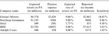
Table 1 illustrates the pension details of selected firms in the sample. The last column estimates the sensitivity of net income to EXPRORPA (i.e., percentage change in net income due to 1% change in EXPRORPA). This measure ranges from 1.83% for Adolph Coors to 14.85% for General Motors and is a function of the pension assets relative to net income. These numbers show the significant impact EXPRORPA has on net income.
2003 footnote disclosures for selected firms

Given the significant impact expected return on pension assets has on earnings and the pressures managers face to meet or exceed analysts' forecasts (DeGeorge et al., Reference DeGeorge, Patel and Zeckhauser1999; Libby and Kinney, Reference Libby and Kinney2000; Brown, Reference Brown2001; Burgstahler and Eames, Reference Burgstahler and Eames2006; Richardson et al., Reference Richardson, Teoh and Wysocki2001) and to avoid reporting earnings declines (Burgstahler and Dichev, Reference Burgstahler and Dichev1997; DeGeorge et al., Reference DeGeorge, Patel and Zeckhauser1999), the paper posits that managers will be tempted to manipulate EXPRORPA to manage earnings to meet or beat market expectations.Footnote 2 Thus the first hypothesis in alternate form is as follows:
H1: Ceteris paribus, managers are likely to report inflated expected rate of return on pension assets when earnings fall short of expectations.
In addition, the paper hypothesizes that the extent of inflation of expected returns on pension assets will be proportional to the amount of shortfall of earnings from expectations and the sensitivity of earnings to expected rate of return on pension assets. Hence, the next two hypotheses state:
H2: Ceteris paribus, the greater the earnings shortfall relative to expectations, the greater the inflation in expected rate of return on pension assets.
H3: Ceteris paribus, the greater the sensitivity of earnings to expected rate of return on pension assets, the greater the inflation in expected rate of return on pension assets.
Finally, if the disclosures under SFAS 87 (FASB, 1985) are adequate, the investors should be able to estimate the extent of earnings manipulations and their resource allocation decisions will not be based on the manipulated component of earnings. Thus, the fourth hypothesis is the following:
H4: Ceteris paribus, investors are able to recognize the manipulated component of earnings and base their resource allocation decisions only on the unmanipulated earnings.
3 Research design
Estimation of the manipulated component of EPS
Two different models are used to remove the effect of manipulated component of EXPRORPA and estimate the unbiased/deflated earnings per share (DEFEPS).
Model I
The following regression that relates reported earnings per share (REPEPS) to EXPRORPA and pension assets per share at the beginning of the fiscal year (PENASSET) is first estimatedFootnote 3

where ‘α’ are the regression coefficients and ‘error’ denotes other information. Prior research (Holthausen, Larcker, and Sloan, Reference Holthausen, Larcker and Sloan1995; Amir and Gordon, Reference Amir and Gordon1996; Asthana, Reference Asthana1999 and Reference Asthana2001) uses the mean of accounting choices for the population of firms as a proxy for the non-discretionary (unmanaged) component of the managerial choice. In line with this research, this model uses the mean EXPRORPA of the population of firms in that year as a proxy for the non-discretionary EXPRORPA. Thus, the deflated component of earnings per share (DEFEPS) can be estimated from equation (1) by replacing EXPRORPA by MNEXPRORPA, the mean EXPRORPA for the sample of firms in that year.

Subtracting equation (1) from (2) yields

where αe denote regression coefficients estimated from regression (1).
Finally the inflated component of earnings per share (INFLATION) can be estimated from equation (3) as

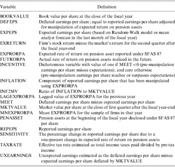
These variables and those defined subsequently are summarized alphabetically in Table 2.
Variable definitions (in alphabetical order)

Model II
This model estimates the manipulated after-tax return on pension assets using MNEXPRORPA and removes it from the REPEPS to get DEFEPS and INFLATION as follows

where TAXRATE is the effective tax rate estimated as the total income taxes paid deflated by pre-tax income. The variable is winsorized in the range [0, 40%] to remove the effect of outliers.
Measure of earnings management incentive
A variable MEET is defined as DEFEPS minus EXPEPS (expected earnings per share). Thus if the unbiased DEFEPS is $1 per share and EXPEPS is $2 per share, MEET is −$1 per share, that is the unmanipulated EPS will miss the expected EPS by $1. A positive (zero) MEET implies that the firm beats (meets) the expectation. Firms with more negative (positive) MEET have more (less) incentives to manage earnings. A dichotomous variable INCENTIVE captures the opportunity set of managers. For firms with MEET<0, INCENTIVE=1; and INCENTIVE=0, otherwise. Two measures of EXPEPS are used. One is the random-walk measure that uses last year's earnings per share as this year's expectation. The other is the mean analyst forecast for the annual earnings per share in the 30 days preceding the earnings disclosure.Footnote 4
Test of hypothesis 1
Hypothesis 1 suggests that firms with greater incentives to manipulate earnings will make more aggressive (optimistic) assumptions regarding EXPRORPA. In other words, one expects that firms with INCENTIVE=1 (=0) will have higher (lower) EXPRORPA and INFLATION. Thus, two measures of INCENTIVE combined with two measures of INFLATION yield four different combinations. Portfolio tests are used to test this hypothesis.
Test of hypotheses 2 and 3
Hypotheses 2 and 3 suggest that EXPRORPA will be decreasing in MEET and increasing in sensitivity of earnings to EXPRORPA. A variable SENSITIVITY that measures the effect of 1% increase in EXPRORPA on $1 after-tax earnings per share is defined as below

The following regression is now run

where ‘β’ are the regression coefficients and LAGEXPRORPA is the lagged EXPRORPA for the previous year; MNEXPRORPA is as defined before; FUTRORPA is the actual rate of return on pension assets realized in the future (one year ahead). These three variables are controls for the unbiased component of EXPRORPA. LAGEXPRORPA controls for non-opportunistic firm-specific choice of EXPRORPA that may be correlated with the allocation of pension assets across various risk categories (that is, riskiness of the pension portfolio). MNEXPRORPA controls for any economy-wide fluctuations in future expected returns. Finally, Amir and Benartzi (Reference Amir and Benartzi1998) find that future actual returns on pension assets are significantly positively correlated with the current pension asset composition. The paper, therefore, uses FUTRORPA as a proxy for the current pension asset composition. Together, LAGEXPRORPA and FUTRORPA, control for the association between EXPRORPA and the actual composition of the pension portfolio. Hypothesis 2 predicts that in equation (5), β4<0 and hypothesis 3 predicts β5>0. Extant literature and pension economics suggest that β1>0, β2>0, and β3>0.
Tests of Hypothesis 4
Hypothesis 4 postulates that investors' resource allocation decisions will not depend on the manipulated component of earnings. In other words, the market value of the firm should reflect the information contained in REPEPS subsequent to the 10-K disclosure after removing the effects of the manipulated component INFLATION. Since firms' have 90 days from the fiscal year-end to issue the 10-K, a variable MKTVALUE is defined as the market value per share on the last day of quarter 1. The following extension of Ohlson's (Reference Ohlson1995) model is run to efficiency hypothesis.
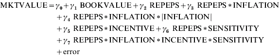
where BOOKVALUE is the book value per share of the firm at the close of the fiscal year. The rest of the variables are as defined above. The coefficients γ0, γ1, and γ2 in equation (6) are predicted to be positive by Ohlson's Model. An efficient market will, however, discount REPEPS for INFLATION (γ3<0); extremely large INFLATION (γ4<0); INCENTIVE (γ5<0); and SENSITIVITY (γ6<0). The last term controls for any interaction effects between INFLATION, INCENTIVE, and SENSITIVITY.
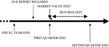
Equation (6) does test for market adjustment for INFLATION, INCENTIVE, and SENSITIVITY. However, it does not tell us how complete this adjustment is. If the adjustment for earnings manipulation is complete, the market returns subsequent to the earnings disclosure should not be a function of the manipulated components of earnings. In other words, the investors' resource allocation decisions in quarter 2 of the subsequent fiscal year will not depend on INFLATION. Figure 1 further illustrates this research design on a time line.
Time-line

A variable EXRETURN is defined as the firm's stock return during the second quarter of the fiscal year subsequent to the earnings disclosure, minus the market return for the same period. Consistent with the earnings response literature, unexpected earnings (UXEARNINGS) is defined as DEFEPS minus EXPEPS deflated by MKTVALUE; and INF2MV is defined as INFLATION deflated by MKTVALUE. The following regression is now estimated.

Bernard and Thomas (Reference Bernard and Thomas1989) document that most of the post-earnings announcement drift occurs during the first 60 trading days (about three months) subsequent to the earnings announcement. Since, the majority of firms file their 10-K close to the end of quarter 1 (Asthana and Balsam, Reference Asthana and Balsam2001), the main post-announcement drift to INFLATION will occur in quarter 2.Footnote 5 If the market has efficiently adjusted REPEPS for the effects of INFLATION, the post-earnings drift will only pertain to DEFEPS (λ1>0) and not to INFLATION (λ2≈0). However, if the adjustment is partial, the post-earnings drift will also depend on INFLATION (λ1≈λ2>0).
4 Sample
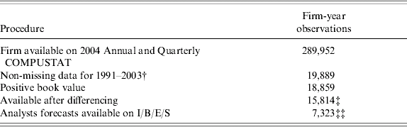
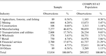
The primary data needed for the tests comes from annual and quarterly COMPUSTAT.Footnote 6 There are 289,952 firm-year observations on 2004 COMPUSTAT. Of these, 19,889 firm year observations have complete data needed for computations for the period 1991–2003.Footnote 7 Only positive BOOKVALUE (18,859) are retained to avoid misspecification of Ohlson's (Reference Ohlson1995) model. After differencing, 15,814 observations from 2,739 firms remain in the sample. Analyst forecasts are obtained from I/B/E/S database and are available for a subset of 1,309 firms (7,323 observations). The sample selection procedure is shown in Table 3 (panel A).
Sample selection and distribution
Panel A: Sample selection
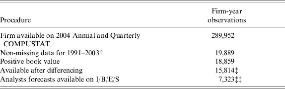
Notes: † COMPUSTAT starts reporting Expected Rate of Return on Pension Assets (data #336) from 1991.
‡ Pertains to 2,739 firms.
‡‡ Pertains to 1,309 firms.
Panel B: Sample distribution across Industries

The industry classification is based on Dopuch et al. (Reference Dopuch, Holthausen and Leftwich1987), and includes the following SIC codes:


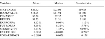
Panel B of Table 3 shows the sample and population distribution across various industries.Footnote 8 Manufacturing is the largest industry (46.02%) and Agriculture, Forestry, and Fishing the lowest (0.56%). Compared to the COMPUSTAT population, Manufacturing and Transportation and Utilities are over-represented, while Financial Services and Services are under-represented. Panel C presents the mean, median, and standard deviation of various variables. Mean (median) MKTVALUE is $26.62 ($23) per share, while BOOKVALUE is $14.25 ($11.94). Mean PENASSET is $5.20 per share and median is $2.32 per share. Firms report a mean $1.33 of earnings per share. The mean (median) EXPRORPA is 8.62% (9%). FUTRORPA has a mean and median of 8.69% and 8.32%, respectively. A 1% increase in EXPRORPA increases the earnings per share by a mean 6.23% (SENSITIVITY).
5 Results
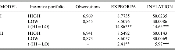
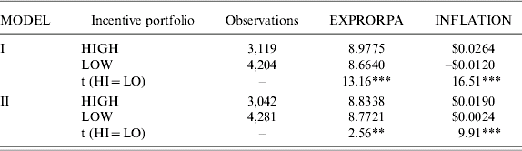
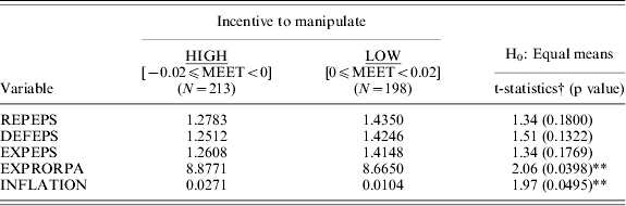
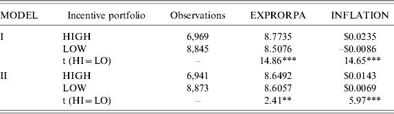
Table 4 exhibits the test for hypothesis 1. Panel A uses random walk expectations for earnings per share. Mean EXPRORPA and INFLATION for the high and low incentive portfolios are reported for both models. The differences are significant in the predicted directions for both variables for each model. Panel B reports the same information using analyst forecasts as expectations for earnings per share and the results are similar to panel A. The results are consistent and support hypothesis 1. Thus, when managers have high incentives to manage earnings (i.e., when they are going to miss the earnings target), they appear to manipulate EXPRORPA upwards and artificially inflate their REPEPS. When such incentives are low for managers (when they are achieving their earning target), they appear to manipulate EXPRORPA and INFLATION significantly less. For the sake of brevity, henceforth, only model 1 results with random-walk expectation are reported. The conclusions for the other combinations are very similar.
Earnings management incentives and selection of expected returns on pension assets
Panel A: Portfolio analysis using random-walk expectation (N=15,814)
Panel B: Portfolio analysis using analysts forecasts as expectation (N=7,323)
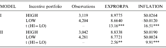
Notes: See Table 2 for variable definitions. High Incentive portfolios have MEET<0 and Low incentives portfolios have MEET⩾0.
† Satterthwaite t-statistics are reported (all variances are significantly different).
*** implies significance at 1% level; ** implies significance at 5% level.
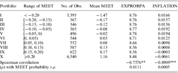
Panels A and B of Table 5 provide more detailed portfolio analysis. Panel A splits the sample into ten portfolios by MEET, with eight of the portfolios focusing on the range ±20 cents of MEET. As predicted by hypothesis 2, EXPRORPA and INFLATION are high for portfolios I to V with MEET<0 (DEFEPS<EXPEPS) and decline as MEET increases (DEFEPS moves towards EXPEPS and then crosses over in portfolio VI). Spearman correlation of EXPRORPA and INFLATION with mean MEET are significantly negative (−0.7576 and −0.8909, respectively).Footnote 9
Selection of expected returns on pension assets:further tests
Panel A: Portfolio analysis

Panel B: Micro-analysis
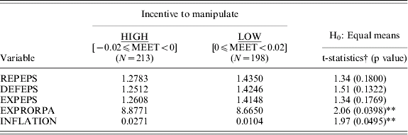
Note: † Satterthwaite t-statistics (all variances are significantly different).
Panel C: Regression tests

Notes: See Table 2 for variable definitions.
*** implies significance at 1% level; ** implies significance at 5% level.
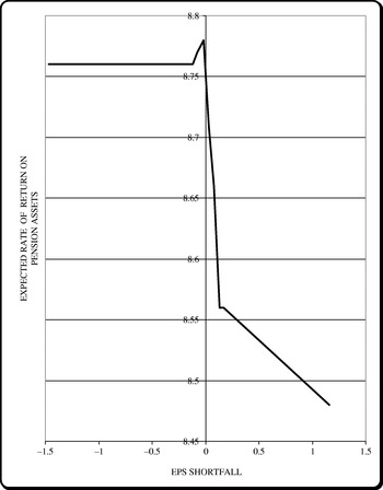
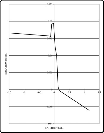
Plots of EXPRORPA and INFLATION with MEET are presented in Figures 2 and 3. The ‘Z’ shaped relationship is consistent with hypotheses 1. The spikes in the two graphs below MEET=0 tell an interesting story. Overall, for MEET<0 the level of EXPRORPA and INFLATION are higher than when MEET is non-negative. However, when MEET is between −12 cents and 0 cents, the managers realize they can actually meet the target and appear to get more aggressive with the manipulation of EXPRORPA, resulting in the spike. Panel B of Table 5 further narrows the range of MEET to ±2 cents and conducts a micro-analysis. For the high incentive portfolio, DEFEPS was missing the target (EXPEPS) by almost a cent. Managers used aggressive choices of EXPRORPA to inflate their earnings by almost 3 cents to beat the target. In the low incentive portfolio DEFEPS was beating the target by almost a cent and the managers only inflated their earnings by a cent. Mean EXPRORPA and INFLATION for the high incentive portfolio are significantly greater than the low incentive portfolio at 5% level. These results provide further support for hypothesis 1.
Plot of expected rate of return on pension assets versus eps shortfall

Plot of earnings management versus eps shortfall

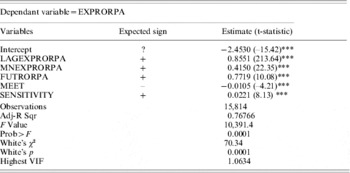
Panel C tests hypotheses 2 and 3 with a regression analysis of equation (5). Coefficients of MEET and SENSITIVITY are significantly negative and positive as expected. Thus as MEET gets more negative (DEFEPS misses EXPEPS by a bigger margin), firms get more desperate and choose more optimistic values of EXPRORPA to inflate their earnings and narrow the gap between REPEPS and EXPEPS. This is consistent with hypothesis 2. The positive sign on SENSITIVITY implies that firms whose earnings are more sensitive to EXPRORPA (high SENSITIVITY) are more likely to choose optimistic values of EXPRORPA to inflate their earnings. This supports hypothesis 3. Coefficients of the control variables, LAGEXPRORPA, MNEXPRORPA, and FUTRORPA are all significantly positive as expected. Regression diagnostics are discussed later in this section.
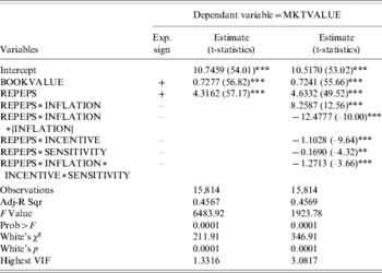
Finally, Table 6 presents tests of hypothesis 4. Panel A reports results of regression (6). A truncated model and the full model are reported. The truncated model only contains the primary variables, BOOKVALUE and REPEPS without controlling for the effects of opportunism. The full model has all the variables described in equation (6). As predicted by Ohlson's (Reference Ohlson1995) model, coefficients of BOOKVALUE and REPEPS are significantly positive in both versions. In the full model, coefficients on REPEPS∗INFLATION∗|INFLATION|, REPEPS∗INCENTIVE, REPEPS∗SENSITIVITY, and REPEPS∗INFLATION∗INCENTIVE∗SENSITIVITY are significantly negative, as predicted. Contrary to expectation, coefficient of REPEPS∗INFLATION is significantly positive. Thus, when firms do not have extremely large INFLATION, INCENTIVE is zero, and SENSITIVITY tends to zero, investors are not skeptical of INFLATION. They treat it as a signal of good management and investment policy that results in higher EXPRORPA. A genuine (not driven by opportunism) increase in EXPRORPA is value adding since it reduces future cash outflow to pension funds, and increases the cash flow to investors. However, when there is evidence of opportunism, very high INFLATION, INCENTIVE>0, and high SENSITIVITY, the investors are skeptical and discount REPEPS accordingly. The last term, REPEPS∗INFLATION∗INCENTIVE∗SENSITIVITY controls for interaction between various variables and is significantly negative. That is, when all variables are non-zero, the market is even more skeptical.
Tests of market efficiency
Panel A: Market value test

Panel B: Returns test (t-statistics in parentheses)

Notes: See Table 2 for variable definitions. *** implies significance at 1% level; ** implies significance at 5% level; * implies significance at 10% level.
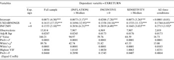
The above regression provides evidence that market is efficient in interpreting SFAS 87 disclosures pertaining to EXPRORPA. However, further tests are needed to ascertain if the adjustment for INFLATION is complete. Panel B reports results of regression (7). If the market has completely removed the effect of INFLATION from REPEPS, post-announcement asset allocation decisions should not depend on INFLATION. The findings, to the contrary, show that EXRETURN depends significantly on both UXEARNINGS and INF2MV, suggesting that INFLATION continues to be value-relevant. Moreover, the coefficient of UNEARNINGS is insignificantly different from INF2MV.
The market may only be skeptical of INFLATION if there is evidence of opportunistic behavior on the part of managers. To examine this possibility, the tests are repeated for sub-samples with high |INFLATION| (values above median), high INCENTIVE (values greater than zero), high SENSITIVITY (values above median), and with high |INFLATION|, INCENTIVE, and SENSITIVITY. The conclusions do not change. These results reject hypothesis 4, suggesting that investors are not able to see through the inflated component of earnings efficiently and continue to base their asset allocation decisions on REPEPS instead of DEFEPS.
Regression diagnostics
The Belsley et al. (Reference Belsley, Kuh and Welsch1980) test for multicollinearity is conducted on regression models (5), (6), and (7), which are reported in Tables 5 and 6. The highest variance inflation factor is 3.0817, below the critical level of 10. Therefore, multicollinearity does not appear to be a significant problem in any of the regression estimations. White's (Reference White1980) test for heteroskedasticity is conducted on all the regressions. The null of homoskedastic errors is rejected in all regressions. Heteroskedasticity corrected t-statistics do not alter the conclusions and are not reported. Diagnostic tests are also conducted for all regressions with influential outliers being removed based on the procedure outlined in Belsley et al. (Reference Belsley, Kuh and Welsch1980). Using SAS, the studentized residual (RSTUDENT) for each observation is calculated. Any observation with an absolute RSTUDENT greater than 2 is deemed to be an influential outlier and deleted (see Belsley et al., Reference Belsley, Kuh and Welsch1980: 28). Removal of outliers does not change the conclusions presented.Footnote 10 Thus the results do not appear to be driven by outliers.
6 Conclusion
This paper empirically examines managers' opportunistic choice of expected rate of return on pension assets with the intent of managing earnings. Results suggest that managers may use aggressive estimates of expected rate of return on pension assets when the earnings are going to miss the earnings targets. The extent of manipulation of expected return on pension assets is directly related to the amount by which the earnings target is going to be missed and the sensitivity of earnings to changes in expected returns. The market appears to partially discount reported earnings for the manipulated component, when managers have incentive and opportunity to manipulate earnings. Subsequent to the earnings disclosure, market participants appear to make their investment decisions on the manipulated earnings rather than the ‘true’ earnings, suggesting that the market impounds the earnings and related pension information inefficiently.
The information provided under SFAS 87 is adequate to empirically estimate the manipulated component of earning. However, the market is unable to evaluate and price this information correctly. One reason could be that the market participants do not have the expertise needed for this estimation. Some additional information can yield enhanced transparency to the earnings and pension disclosures, thereby facilitating proper pricing of earnings and discouraging earnings manipulations. For example, Department of Labor could mandate additional reporting of earnings calculated with a standard expected rate of return on pension assets that could be based on population mean. The firm could then be required to justify the difference between the standardized and reported earnings. This additional reporting will make any earnings differences more visible and put the onus on the firm to explain the reasons for the variation to the investors. Overall, this will increase both the investors' awareness and the managers' risk of cosmetically inflating earnings. If the additional disclosures help the market price out the inflated component from disclosed earnings, this will be an added disincentive for managers to manipulate earnings.
Appendix: Calculation of net periodic pension cost
Under SFAS 87 (FASB, 1985), the net periodic pension cost or pension expense of defined-benefit pension plans consists of service cost, interest cost, amortization of unrecognized prior service cost, amortization of experience loss (gain), minus expected return on pension assets,. The service cost is the expense caused by the increase in projected benefit obligations (PBO) payable to the employees as a result of service rendered during the year. The interest cost is the interest payable on the beginning balance of PBO. Unrecognized prior service costs are additional pension benefits granted for service performed in prior periods. Experience loss (gain) is the deviation of actual amounts from estimated amounts (amortized only if they exceed 10% of the greater of PBO or market-related value of pension assets at the beginning of the year). The expected return on pension assets is EXPRORPA multiplied by the market-related value of pension assets at the beginning of fiscal year. Net periodic pension cost is a decreasing and earnings an increasing function of EXPRORPA. Typically, EXPROPA used is from the current 10-K, while PBO, plan assets, discount rate and compensation rate are from previous year's 10-K.