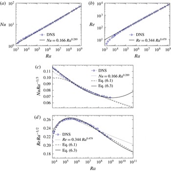
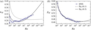
1. Introduction
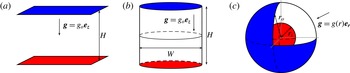
Thermal convection is ubiquitous in geophysical and astrophysical fluid dynamics and determines, for example, the behaviour of turbulent flows in the interiors of planets and stars. The so-called Rayleigh–Bénard (hereafter RB) convection is probably the simplest paradigm to study heat transport phenomena in these natural systems. In this configuration, convection is driven in a planar fluid layer cooled from above and heated from below (figure 1
a). The fluid is confined between two rigid impenetrable walls maintained at constant temperatures. The key issue in RB convection is to understand the turbulent transport mechanisms of heat and momentum across the layer. In particular, how does the heat transport, characterised by the Nusselt number
 $\mathit{Nu}$
, and the flow amplitude, characterised by the Reynolds number
 $\mathit{Re}$
, depend on the various control parameters of the system, namely the Rayleigh number
 $\mathit{Ra}$
, the Prandtl number
 $\mathit{Pr}$
and the Cartesian aspect ratio
 ${\it\Gamma}$
? In general,
 ${\it\Gamma}=W/H$
quantifies the fluid layer width
 $W$
over its height
 $H$
in classical planar or cylindrical RB cells. In spherical shells, we instead employ the ratio of the inner to the outer radius
 ${\it\eta}=r_{i}/r_{o}$
to characterise the geometry of the fluid layer.
Schematic showing different Rayleigh–Bénard convection set-ups. (a) An infinitely extended fluid layer of height
 $H$
heated from below and cooled from above. (b) The typical RB convection set-up in a cylindrical cell of aspect ratio
 ${\it\Gamma}=W/H$
. (c) Convection in a spherical shell with a radius ratio
 ${\it\eta}=r_{i}/r_{o}$
with a radially inward gravity. In the three panels, the red and the blue surfaces correspond to the hot and cold boundaries held at constant temperatures.

Laboratory experiments of RB convection are classically performed in rectangular or in cylindrical tanks with planar upper and lower bounding surfaces where the temperature contrast is imposed (see figure 1
b). In such a system, the global dynamics are strongly influenced by the flow properties in the thermal and kinematic boundary layers that form in the vicinity of the walls. The characterisation of the structure of these boundary layers is crucial for a better understanding of the transport processes. The marginal stability theory of Malkus (Reference Malkus1954) is the earliest boundary layer model and relies on the assumption that the thermal boundary layers adapt their thicknesses to maintain a critical boundary layer Rayleigh number, which implies
 $\mathit{Nu}\sim \mathit{Ra}^{1/3}$
. Assuming that the boundary layers are sheared, Shraiman & Siggia (Reference Shraiman and Siggia1990) later derived a theoretical model that yielded scalings of the form
 $\mathit{Nu}\sim \mathit{Ra}^{2/7}\,\mathit{Pr}^{-1/7}$
and
 $\mathit{Re}\sim \mathit{Ra}^{3/7}\,\mathit{Pr}^{-5/7}$
(see also Siggia Reference Siggia1994). These asymptotic laws were generally consistent with most of the experimental results obtained in the 1990s up to
 $\mathit{Ra}\lesssim 10^{11}$
. Within the typical experimental resolution of 1 %, simple power laws of the form
 $\mathit{Nu}\sim \mathit{Ra}^{{\it\alpha}}\mathit{Pr}^{{\it\beta}}$
were found to provide an adequate representation, with
 ${\it\alpha}$
exponents ranging from 0.28 to 0.31, in relatively good agreement with the Shraiman & Siggia model (e.g. Castaing et al.
Reference Castaing, Gunaratne, Kadanoff, Libchaber and Heslot1989; Chavanne et al.
Reference Chavanne, Chillà, Castaing, Hébral, Chabaud and Chaussy1997; Niemela et al.
Reference Niemela, Skrbek, Sreenivasan and Donnelly2000). However, later high-precision experiments by Xu, Bajaj & Ahlers (Reference Xu, Bajaj and Ahlers2000) revealed that the dependence of
 $\mathit{Nu}$
upon
 $\mathit{Ra}$
cannot be accurately described by such simple power laws. In particular, the local slope of the function
 $\mathit{Nu}(\mathit{Ra})$
has been found to increase slowly with
 $\mathit{Ra}$
. The effective exponent
 ${\it\alpha}_{eff}$
of
 $\mathit{Nu}\sim \mathit{Ra}^{{\it\alpha}_{eff}}$
ranges approximately from values close to 0.28 near
 $\mathit{Ra}\sim 10^{7}{-}10^{8}$
, to 0.33 when
 $\mathit{Ra}\sim 10^{11}{-}10^{12}$
(e.g. Funfschilling et al.
Reference Funfschilling, Brown, Nikolaenko and Ahlers2005; Cheng et al.
Reference Cheng, Stellmach, Ribeiro, Grannan, King and Aurnou2015).
Grossmann & Lohse (Reference Grossmann and Lohse2000, Reference Grossmann and Lohse2004) derived a competing theory capable of capturing this complex dynamics (hereafter GL). This scaling theory is built on the assumption of laminar boundary layers of a Prandtl–Blasius (PB) type (Prandtl Reference Prandtl1905; Blasius Reference Blasius1908). According to the GL theory, the flows are classified into four different regimes in the
 $\mathit{Ra}{-}\mathit{Pr}$
phase space according to the relative contribution of the bulk and boundary layer viscous and thermal dissipation rates. The theory predicts non-power-law behaviours for
 $\mathit{Nu}$
and
 $\mathit{Ra}$
, in good agreement with the dependence
 $\mathit{Nu}=f(\mathit{Ra},\mathit{Pr},{\it\Gamma})$
and
 $\mathit{Re}=f(\mathit{Ra},\mathit{Pr},{\it\Gamma})$
observed in recent experiments and numerical simulations of RB convection in planar or cylindrical geometries (see for recent reviews Ahlers, Grossmann & Lohse Reference Ahlers, Grossmann and Lohse2009; Chillà & Schumacher Reference Chillà and Schumacher2012).
Benefiting from the interplay between experiments and direct numerical simulations (DNS), turbulent RB convection in planar and cylindrical cells has received a lot of interest in the past two decades. However, the actual geometry of several fundamental astrophysical and geophysical flows is essentially three-dimensional within concentric spherical upper and lower bounding surfaces under the influence of a radial buoyancy force that strongly depends on radius. The direct applicability of the results derived in the planar geometry to spherical shell convection is thus questionable.
As shown in figure 1(c), convection in spherical shells mainly differs from the traditional plane layer configuration because of the introduction of curvature and the absence of side walls. These specific features of thermal convection in spherical shells yield significant dynamical differences with plane layers. For instance, the heat flux conservation through spherical surfaces implies that the temperature gradient is larger at the lower boundary than at the upper one to compensate for the smaller area of the bottom surface. This yields a much larger temperature drop at the inner boundary than at the outer one. In addition, this pronounced asymmetry in the temperature profile is accompanied by a difference between the thicknesses of the inner and the outer thermal boundary layers. Following Malkus’s marginal stability arguments, Jarvis (Reference Jarvis1993) and Vangelov & Jarvis (Reference Vangelov and Jarvis1994) hypothesised that the thermal boundary layers in curvilinear geometries adjust their thickness to maintain the same critical boundary layer Rayleigh number at both boundaries. This criterion is however in poor agreement with the results from numerical models (e.g. Deschamps, Tackley & Nakagawa Reference Deschamps, Tackley and Nakagawa2010). The exact dependence of the boundary layer asymmetry on the radius ratio and the gravity distribution thus remains an open question for thermal convection in spherical shells (Bercovici et al. Reference Bercovici, Schubert, Glatzmaier and Zebib1989; Jarvis, Glatzmaier & Vangelov Reference Jarvis, Glatzmaier and Vangelov1995; Sotin & Labrosse Reference Sotin and Labrosse1999; Shahnas et al. Reference Shahnas, Lowman, Jarvis and Bunge2008; O’Farrell, Lowman & Bunge Reference O’Farrell, Lowman and Bunge2013). This open issue sheds some light on the possible dynamical influence of asymmetries between the hot and cold surfaces that originate due to both the boundary curvature and the radial dependence of buoyancy in spherical shells.
Ground-based laboratory experiments involving spherical geometry and a radial buoyancy forcing are limited by the fact that gravity acts vertically downwards instead of radially inwards (Scanlan, Bishop & Powe Reference Scanlan, Bishop and Powe1970; Feldman & Colonius Reference Feldman and Colonius2013). A possible way to circumvent this limitation is to conduct experiments under microgravity to suppress the vertically downward buoyancy force. Such an experiment was realised by Hart, Glatzmaier & Toomre (Reference Hart, Glatzmaier and Toomre1986) who designed a hemispherical shell that flew on board the space shuttle Challenger in May 1985. The radial buoyancy force was modelled by imposing an electric field across the shell. The temperature dependence of the fluid’s dielectric properties then produced an effective radial gravity that decreased with the fifth power of the radius (i.e.
 $g\sim 1/r^{5}$
). More recently, a similar experiment named ‘GeoFlow’ was run on the International Space Station, where much longer flight times are possible (Futterer et al.
Reference Futterer, Egbers, Dahley, Koch and Jehring2010, Reference Futterer, Krebs, Plesa, Zaussinger, Hollerbach, Breuer and Egbers2013). This later experiment was designed to mimic the physical conditions in the Earth’s mantle. It was therefore mainly dedicated to the observation of plume-like structures in a high Prandtl number regime (
 $\mathit{Pr}>40$
) for
 $\mathit{Ra}\leqslant 10^{6}$
. Unfortunately, this limitation to relatively small Rayleigh numbers makes the GeoFlow experiment quite restricted regarding asymptotic scaling behaviours in spherical shells.
To compensate for the lack of laboratory experiments, three-dimensional numerical models of convection in spherical shells have been in development since the 1980s (e.g. Zebib, Schubert & Straus Reference Zebib, Schubert and Straus1980; Bercovici et al.
Reference Bercovici, Schubert, Glatzmaier and Zebib1989; Bercovici, Schubert & Glatzmaier Reference Bercovici, Schubert and Glatzmaier1992; Jarvis et al.
Reference Jarvis, Glatzmaier and Vangelov1995; Tilgner Reference Tilgner1996; Tilgner & Busse Reference Tilgner and Busse1997; King et al.
Reference King, Soderlund, Christensen, Wicht and Aurnou2010; Choblet Reference Choblet2012). The vast majority of the numerical models of non-rotating convection in spherical shells have been developed with the Earth’s mantle in mind. These models therefore assume an infinite Prandtl number and most of them further include a strong dependence of viscosity on temperature to mimic the complex rheology of the mantle. Several recent studies of isoviscous convection with infinite Prandtl number in spherical shells have nevertheless been dedicated to the analysis of the scaling properties of the Nusselt number. For instance, Deschamps et al. (Reference Deschamps, Tackley and Nakagawa2010) measured convective heat transfer in various radius ratios ranging from
 ${\it\eta}=0.3$
to
 ${\it\eta}=0.8$
and reported
 $\mathit{Nu}\sim \mathit{Ra}^{0.273}$
for
 $10^{4}\leqslant \mathit{Ra}\leqslant 10^{7}$
, while Wolstencroft, Davies & Davies (Reference Wolstencroft, Davies and Davies2009) computed numerical models with the Earth’s mantle geometry (
 ${\it\eta}=0.55$
) up to
 $\mathit{Ra}=10^{8}$
and found
 $\mathit{Nu}\sim \mathit{Ra}^{0.294}$
. These studies also investigated the possible influence of internal heating and reported quite similar scalings.
Most of the numerical models of convection in spherical shells have thus focused on the very specific dynamical regime of infinite Prandtl number. The most recent attempt to derive the scaling properties of
 $\mathit{Nu}$
and
 $\mathit{Re}$
in non-rotating spherical shells with finite Prandtl numbers is the study of Tilgner (Reference Tilgner1996). He studied convection in self-gravitating spherical shells (i.e.
 $g\sim r$
) with
 ${\it\eta}=0.4$
spanning the range
 $0.06\leqslant \mathit{Pr}\leqslant 10$
and
 $4\times 10^{3}\leqslant \mathit{Ra}\leqslant 8\times 10^{5}$
. This study was thus restricted to low Rayleigh numbers relatively close to the onset of convection, which prevents the derivation of asymptotic scalings for
 $\mathit{Nu}(\mathit{Ra},\mathit{Pr})$
and
 $\mathit{Re}(\mathit{Ra},\mathit{Pr})$
in spherical shells.
The objectives of the present work are twofold: (i) to study the scaling properties of
 $\mathit{Nu}$
and
 $\mathit{Re}$
in spherical shells with finite Prandtl number; (ii) to better characterise the inherent asymmetric boundary layers for thermal convection in spherical shells. We therefore conduct two systematic parameter studies of turbulent RB convection in spherical shells with
 $\mathit{Pr}=1$
by means of three-dimensional DNS. In the first set of models, we vary both the radius ratio (from
 ${\it\eta}=0.2$
to
 ${\it\eta}=0.95$
) and the radial gravity profile (considering
 $g(r)\in [r/r_{o},1,(r_{o}/r)^{2},(r_{o}/r)^{5}]$
) in a moderate parameter regime (i.e.
 $5\leqslant Nu\leqslant 15$
for the majority of the cases) to study the influence of these properties on the boundary layer asymmetry. We then consider a second set of models with
 ${\it\eta}=0.6$
and
 $g\sim 1/r^{2}$
up to
 $\mathit{Ra}=10^{9}$
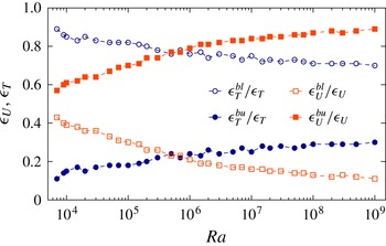
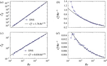
. These DNS are used to check the applicability of the GL theory to thermal convection in spherical shells. We therefore numerically test the different basic prerequisites of the GL theory: we first analyse the nature of the boundary layers before deriving the individual scaling properties for the different contributions to the viscous and thermal dissipation rates.
The paper is organised as follows. In § 2, we present the governing equations and the numerical models. We then focus on the asymmetry of the thermal boundary layers in § 3. In § 4, we analyse the nature of the boundary layers and show that the boundary layer profiles are in agreement with the Prandtl–Blasius theory (Prandtl Reference Prandtl1905; Blasius Reference Blasius1908). In § 5, we investigate the scaling properties of the viscous and thermal dissipation rates before calculating the
 $\mathit{Nu}(\mathit{Ra})$
and
 $\mathit{Re}(\mathit{Ra})$
scalings in § 6. We conclude with a summary of our findings in § 7.
2. Model formulation
2.1. Governing hydrodynamical equations
We consider RB convection of a Boussinesq fluid contained in a spherical shell of outer radius
 $r_{o}$
and inner radius
 $r_{i}$
. The boundaries are impermeable, no-slip, and at constant temperatures
 $T_{bot}$
and
 $T_{top}$
. We adopt a dimensionless formulation using the shell gap
 $d=r_{o}-r_{i}$
as the reference length scale and the viscous dissipation time
 $d^{2}/{\it\nu}$
as the reference timescale. Temperature is given in units of
 ${\rm\Delta}T=T_{top}-T_{bot}$
, the imposed temperature contrast over the shell. Velocity and pressure are expressed in units of
 ${\it\nu}/d$
and
 ${\it\rho}_{o}{\it\nu}^{2}/d^{2}$
, respectively. Gravity is non-dimensionalised using its reference value at the outer boundary
 $g_{o}$
. The dimensionless equations for the velocity
 $\boldsymbol{u}$
, the pressure
 $p$
and the temperature
 $T$
are given by
 $$\begin{eqnarray}\displaystyle & \boldsymbol{{\rm\nabla}}\boldsymbol{\cdot }\boldsymbol{u}=0, & \displaystyle\end{eqnarray}$$
 $$\begin{eqnarray}\displaystyle & \displaystyle \frac{\partial \boldsymbol{u}}{\partial t}+\boldsymbol{u}\boldsymbol{\cdot }\boldsymbol{{\rm\nabla}}\boldsymbol{u}=-\boldsymbol{{\rm\nabla}}p+\frac{\mathit{Ra}}{\mathit{Pr}}\,g\,T\,\boldsymbol{e}_{\boldsymbol{r}}+{\bf\Delta}\boldsymbol{u}, & \displaystyle\end{eqnarray}$$
 $$\begin{eqnarray}\displaystyle & \displaystyle \frac{\partial T}{\partial t}+\boldsymbol{u}\boldsymbol{\cdot }\boldsymbol{{\rm\nabla}}T=\frac{1}{\mathit{Pr}}{\rm\Delta}T, & \displaystyle\end{eqnarray}$$
 $\boldsymbol{e}_{r}$
is the unit vector in the radial direction and
 $g$
is gravity. Several gravity profiles have been classically considered to model convection in spherical shells. For instance, self-gravitating spherical shells with a constant density correspond to
 $g\sim r$
(e.g. Tilgner Reference Tilgner1996), while RB convection models with infinite Prandtl number usually assume a constant gravity in the perspective of modelling Earth’s mantle (e.g. Bercovici et al.
Reference Bercovici, Schubert, Glatzmaier and Zebib1989). The assumption of a centrally condensed mass has also been frequently assumed when modelling rotating convection (e.g. Gilman & Glatzmaier Reference Gilman and Glatzmaier1981; Jones et al.
Reference Jones, Boronski, Brun, Glatzmaier, Gastine, Miesch and Wicht2011) and yields
 $g\sim 1/r^{2}$
. Finally, the artificial central force field of the microgravity experiments effectively takes the form of
 $g\sim 1/r^{5}$
(Hart et al.
Reference Hart, Glatzmaier and Toomre1986; Feudel et al.
Reference Feudel, Bergemann, Tuckerman, Egbers, Futterer, Gellert and Hollerbach2011; Futterer et al.
Reference Futterer, Krebs, Plesa, Zaussinger, Hollerbach, Breuer and Egbers2013). To explore the possible impact of these various radial distributions of buoyancy on RB convection in spherical shells, we consider different models with the four following gravity profiles:
 $g\in [r/r_{o},\,1,\,(r_{o}/r)^{2},\,(r_{o}/r)^{5}]$
. Particular attention will be paid to the cases with
 $g=(r_{o}/r)^{2}$
, which is the only radial function compatible with an exact analysis of the dissipation rates (see below, § 2.3).
The dimensionless set of (2.1)–(2.3) is governed by the Rayleigh number
 $\mathit{Ra}$
, the Prandtl number
 $\mathit{Pr}$
and the radius ratio of the spherical shell
 ${\it\eta}$
defined by
 $$\begin{eqnarray}\mathit{Ra}=\frac{{\it\alpha}g_{o}{\rm\Delta}Td^{3}}{{\it\nu}{\it\kappa}},\quad \mathit{Pr}=\frac{{\it\nu}}{{\it\kappa}},\quad {\it\eta}=\frac{r_{i}}{r_{o}},\end{eqnarray}$$
where
 ${\it\nu}$
and
 ${\it\kappa}$
are the viscous and thermal diffusivities and
 ${\it\alpha}$
is the thermal expansivity.
2.2. Diagnostic parameters
To quantify the impact of the different control parameters on the transport of heat and momentum, we analyse several diagnostic properties. We adopt the following notations regarding different averaging procedures. Overbars
 $\overline{\cdots \,}$
correspond to a time average
 $$\begin{eqnarray}\overline{f}={\displaystyle \frac{1}{{\it\tau}}}\int _{t_{0}}^{t_{0}+{\it\tau}}f\,\text{d}t,\end{eqnarray}$$
where
 ${\it\tau}$
is the time averaging interval. Spatial averaging over the whole volume of the spherical shell is denoted by triangular brackets
 $\langle \cdots \!\,\rangle$
, while
 $\langle \cdots \!\,\rangle _{s}$
correspond to an average over a spherical surface:
 $$\begin{eqnarray}\left\langle f\right\rangle =\frac{1}{V}\int _{V}f(r,{\it\theta},{\it\phi})\,\text{d}V;\quad \left\langle f\right\rangle _{s}=\frac{1}{4{\rm\pi}}\int _{0}^{{\rm\pi}}\int _{0}^{2{\rm\pi}}f(r,{\it\theta},{\it\phi})\sin {\it\theta}\,\text{d}{\it\theta}\,\text{d}{\it\phi},\end{eqnarray}$$
where
 $V$
is the volume of the spherical shell,
 $r$
is the radius,
 ${\it\theta}$
the colatitude and
 ${\it\phi}$
the longitude.
The convective heat transport is characterised by the Nusselt number
 $\mathit{Nu}$
, the ratio of the total heat flux to the heat carried by conduction. In spherical shells with isothermal boundaries, the conductive temperature profile
 $T_{c}$
is the solution of
 $$\begin{eqnarray}\frac{\text{d}}{\text{d}r}\left(r^{2}\frac{\text{d}T_{c}}{\text{d}r}\right)=0,\quad T_{c}(r_{i})=1,\quad T_{c}(r_{o})=0,\end{eqnarray}$$
which yields
 $$\begin{eqnarray}T_{c}(r)=\frac{{\it\eta}}{(1-{\it\eta})^{2}}\frac{1}{r}-\frac{{\it\eta}}{1-{\it\eta}}.\end{eqnarray}$$
For the sake of clarity, we adopt in the following the notation
 ${\it\vartheta}$
for the time-averaged and horizontally averaged radial temperature profile:
 $$\begin{eqnarray}{\it\vartheta}(r)=\overline{\left\langle T\right\rangle _{s}}.\end{eqnarray}$$
The Nusselt number then reads
 $$\begin{eqnarray}\mathit{Nu}=\frac{\displaystyle \overline{\left\langle u_{r}T\right\rangle _{s}}-\frac{1}{\mathit{Pr}}\frac{\text{d}{\it\vartheta}}{\text{d}r}}{\displaystyle -\frac{1}{\mathit{Pr}}\frac{\text{d}T_{c}}{\text{dr}}}=-{\it\eta}\frac{\text{d}{\it\vartheta}}{\text{d}r}(r=r_{i})=-\frac{1}{{\it\eta}}\frac{\text{d}{\it\vartheta}}{\text{d}r}(r=r_{o}).\end{eqnarray}$$
The typical root-mean-square (r.m.s.) flow velocity is given by the Reynolds number
 $$\begin{eqnarray}\mathit{Re}=\overline{\sqrt{\langle u^{2}\rangle }}=\overline{\sqrt{\langle u_{r}^{2}+u_{{\it\theta}}^{2}+u_{{\it\phi}}^{2}\rangle }},\end{eqnarray}$$
while the radial profile for the time and horizontally averaged horizontal velocity is defined by
 $$\begin{eqnarray}\mathit{Re}_{h}(r)=\overline{\left\langle \sqrt{u_{{\it\theta}}^{2}+u_{{\it\phi}}^{2}}\right\rangle _{s}}.\end{eqnarray}$$
2.3. Exact dissipation relationships in spherical shells
The mean buoyancy power averaged over the whole volume of a spherical shell is expressed by
 $$\begin{eqnarray}P=\frac{\mathit{Ra}}{\mathit{Pr}}\,\overline{\left\langle g\,u_{r}T\right\rangle }=\frac{4{\rm\pi}}{V}\,\frac{\mathit{Ra}}{\mathit{Pr}}\int _{r_{i}}^{r_{o}}g\,r^{2}\,\overline{\left\langle u_{r}T\right\rangle _{s}}\,\text{d}r.\end{eqnarray}$$
Using the Nusselt number definition (2.10) and the conductive temperature profile (2.8) then leads to
 $$\begin{eqnarray}P=\frac{4{\rm\pi}}{V}\,\frac{\mathit{Ra}}{\mathit{Pr}^{2}}\left(\int _{r_{i}}^{r_{o}}g\,r^{2}\,{\displaystyle \frac{\text{d}{\it\vartheta}}{\text{d}r}}\,\text{d}r-Nu\,\frac{{\it\eta}}{(1-{\it\eta})^{2}}\int _{r_{i}}^{r_{o}}g\,\text{d}r\right).\end{eqnarray}$$
The first term in the parentheses becomes identical to the imposed temperature drop
 ${\rm\Delta}T$
for a gravity
 $g\sim 1/r^{2}$
:
 $$\begin{eqnarray}\int _{r_{i}}^{r_{o}}g\,r^{2}\,{\displaystyle \frac{\text{d}{\it\vartheta}}{\text{d}r}}\,\text{d}r=r_{o}^{2}[{\it\vartheta}(r_{o})-{\it\vartheta}(r_{i})]=-r_{o}^{2},\end{eqnarray}$$
and thus yields an analytical relation between
 $P$
and
 $\mathit{Nu}$
. For any other gravity model, we have to consider the actual spherically symmetric radial temperature profile
 ${\it\vartheta}(r)$
. Christensen & Aubert (Reference Christensen and Aubert2006) solve this problem by approximating
 ${\it\vartheta}(r)$
by the diffusive solution (2.8) and obtain an approximate relation between
 $P$
and
 $(Ra/\mathit{Pr}^{2})(\mathit{Nu}-1)$
. This motivates our particular focus on the
 $g=(r_{o}/r)^{2}$
cases which allows us to conduct an exact analysis of the dissipation rates and therefore check the applicability of the GL theory to convection in spherical shells.
Noting that
 $({\it\eta}/(1-{\it\eta})^{2})\int _{r_{i}}^{r_{o}}g\,\text{d}r=-1/(1-{\it\eta})^{2}$
for
 $g=(r_{o}/r)^{2}$
, one finally obtains the exact relation for the viscous dissipation rate
 ${\it\epsilon}_{U}$
:
 $$\begin{eqnarray}{\it\epsilon}_{U}=\overline{\left\langle (\boldsymbol{{\rm\nabla}}\times \boldsymbol{u})^{2}\right\rangle }=P={\displaystyle \frac{3}{1+{\it\eta}+{\it\eta}^{2}}}\,\frac{\mathit{Ra}}{\mathit{Pr}^{2}}\,(\mathit{Nu}-1).\end{eqnarray}$$
The thermal dissipation rate can be obtained by multiplying the temperature equation (2.3) by
 $T$
and integrating over the whole volume of the spherical shell. This yields
 $$\begin{eqnarray}{\it\epsilon}_{T}=\overline{\left\langle ({\rm\nabla}T)^{2}\right\rangle }={\displaystyle \frac{3{\it\eta}}{1+{\it\eta}+{\it\eta}^{2}}}\,\mathit{Nu}.\end{eqnarray}$$
These two exact relations (2.16) and (2.17) can be used to validate the spatial resolutions of the numerical models with
 $g=(r_{o}/r)^{2}$
. To do so, we introduce
 ${\it\chi}_{{\it\epsilon}_{U}}$
and
 ${\it\chi}_{{\it\epsilon}_{T}}$
, the ratios of the two sides of (2.16) and (2.17):
 $$\begin{eqnarray}\left.\begin{array}{@{}c@{}}\displaystyle {\it\chi}_{{\it\epsilon}_{U}}=\frac{(1+{\it\eta}+{\it\eta}^{2})\,\mathit{Pr}^{2}}{3\,Ra\,(\mathit{Nu}-1)}\,{\it\epsilon}_{U},\\ \displaystyle {\it\chi}_{{\it\epsilon}_{T}}=\frac{(1+{\it\eta}+{\it\eta}^{2})}{3{\it\eta}\,\mathit{Nu}}\,{\it\epsilon}_{T}.\end{array}\right\}\end{eqnarray}$$
2.4. Setting up a parameter study
2.4.1. Numerical technique
The numerical simulations have been carried out with the magnetohydrodynamics code MagIC (Wicht Reference Wicht2002). MagIC has been validated via several benchmark tests for convection and dynamo action (Christensen et al. Reference Christensen, Aubert, Cardin, Dormy, Gibbons, Glatzmaier, Grote, Honkura, Jones, Kono, Matsushima, Sakuraba, Takahashi, Tilgner, Wicht and Zhang2001; Jones et al. Reference Jones, Boronski, Brun, Glatzmaier, Gastine, Miesch and Wicht2011). To solve the system of (2.1)–(2.3), the solenoidal velocity field is decomposed into a poloidal and a toroidal contribution
 $$\begin{eqnarray}\boldsymbol{u}=\boldsymbol{{\rm\nabla}}\times (\boldsymbol{{\rm\nabla}}\times W\boldsymbol{e}_{\boldsymbol{r}})+\boldsymbol{{\rm\nabla}}\times Z\boldsymbol{e}_{\boldsymbol{r}},\end{eqnarray}$$
where
 $W$
and
 $Z$
are the poloidal and toroidal potentials.
 $W$
,
 $Z$
,
 $p$
and
 $T$
are then expanded in spherical harmonic functions up to degree
 $\ell _{max}$
in the angular variables
 ${\it\theta}$
and
 ${\it\phi}$
and in Chebyshev polynomials up to degree
 $N_{r}$
in the radial direction. The combined equations governing
 $W$
and
 $p$
are obtained by taking the radial component and the horizontal part of the divergence of (2.2). The equation for
 $Z$
is obtained by taking the radial component of the curl of (2.2). The equations are time stepped by advancing the nonlinear terms using an explicit second-order Adams–Bashforth scheme, while the linear terms are time advanced using an implicit Crank–Nicolson algorithm. At each time step, all the nonlinear products are calculated in the physical space (
 $r$
,
 ${\it\theta}$
,
 ${\it\phi}$
) and transformed back into the spectral space (
 $r$
,
 $\ell$
,
 $m$
). For more detailed descriptions of the numerical method and the associated spectral transforms, the reader is referred to (Gilman & Glatzmaier Reference Gilman and Glatzmaier1981; Tilgner & Busse Reference Tilgner and Busse1997; Christensen & Wicht Reference Christensen, Wicht and Olson2007).
2.4.2. Parameter choices
One of the main focuses of this study is to investigate the global scaling properties of
 $\mathit{Pr}=1$
RB convection in spherical shell geometries. This is achieved via measurements of the Nusselt and Reynolds numbers. In particular, we aim to test the applicability of the GL theory to spherical shells. As previously demonstrated, only the particular choice of a gravity profile of the form
 $g\sim 1/r^{2}$
allows for an exact definition of the relation (2.16). Our main set of simulations is thus built assuming
 $g=(r_{o}/r)^{2}$
. The radius ratio is kept to
 ${\it\eta}=0.6$
and the Prandtl number to
 $\mathit{Pr}=1$
to allow future comparisons with the rotating convection models of Gastine & Wicht (Reference Gastine and Wicht2012) and Gastine, Wicht & Aurnou (Reference Gastine, Wicht and Aurnou2013) who adopted the same configuration. We consider 35 numerical cases spanning the range
 $1.5\times 10^{3}\leqslant \mathit{Ra}\leqslant 10^{9}$
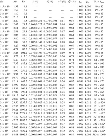
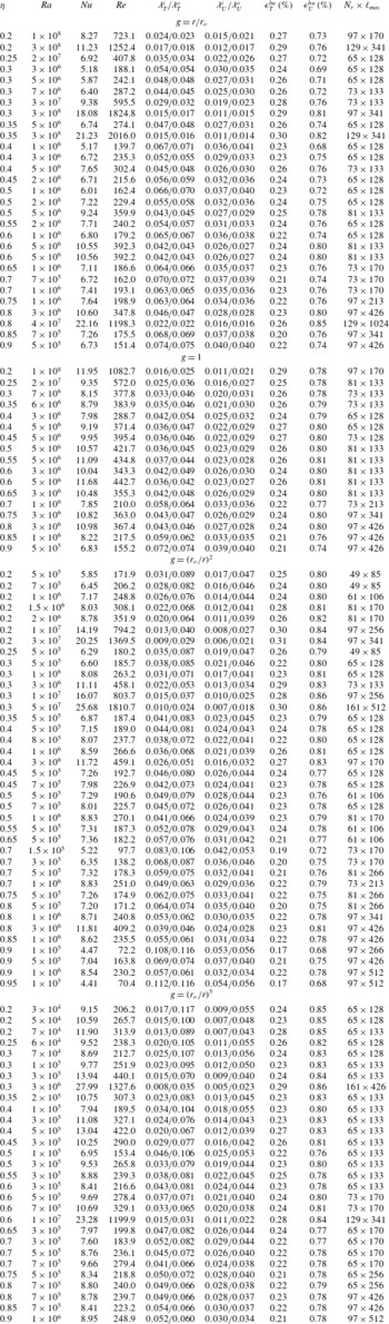
. Table 1 summarises the main diagnostic quantities for this dataset of numerical simulations and shows that our models essentially lie within the ranges
 $1<\mathit{Re}<7000$
and
 $1<Nu<70$
.
Summary table of
 $\mathit{Pr}=1$
numerical simulations with
 ${\it\eta}=0.6$
and
 $g=(r_{o}/r)^{2}$
. The boundary layer thicknesses and the viscous and thermal dissipations are only given for the cases with
 $\mathit{Ra}\geqslant 7\times 10^{3}$
where boundary layers can be clearly identified. The italic lines indicate simulations with smaller truncations to highlight possible resolution problems. The cases with
 $\mathit{Ra}=5\times 10^{8}$
and
 $\mathit{Ra}=10^{9}$
(highlighted with a star in the last column) have been computed assuming a twofold symmetry, i.e. effectively simulating only half of the spherical shell in longitude.

Another important issue in convection in spherical shells concerns the determination of the average bulk temperature and possible boundary layer asymmetry between the inner and the outer boundaries (e.g. Jarvis Reference Jarvis1993; Tilgner Reference Tilgner1996). To better understand the influence of curvature and the radial distribution of buoyancy, we thus compute a second set of numerical models. This additional dataset consists of 113 additional simulations with various radius ratios and gravity profiles, spanning the range
 $0.2\leqslant {\it\eta}\leqslant 0.95$
with
 $g\in [r/r_{o},\,1,\,(r_{o}/r)^{2},\,(r_{o}/r)^{5}]$
. To limit the numerical cost of this second dataset, these cases have been run at moderate Rayleigh number and typically span the range
 $5<Nu<15$
for the majority of the cases. Table 2, given in the appendix A, summarises the main diagnostic quantities for this second dataset of numerical simulations.
2.4.3. Resolution checks
Attention must be paid to the numerical resolutions of the DNS of RB convection (e.g. Shishkina et al.
Reference Shishkina, Stevens, Grossmann and Lohse2010). In particular, failing to properly resolve the fine structure of the turbulent flow leads to an overestimate of the Nusselt number, which then falsifies the possible scaling analysis (Amati et al.
Reference Amati, Koal, Massaioli, Sreenivasan and Verzicco2005). One of the most reliable ways to validate the truncations employed in our numerical models consists of comparing the obtained viscous and thermal dissipation rates with the average Nusselt number (Stevens, Verzicco & Lohse Reference Stevens, Verzicco and Lohse2010; King, Stellmach & Aurnou Reference King, Stellmach and Aurnou2012; Lakkaraju et al.
Reference Lakkaraju, Stevens, Verzicco, Grossmann, Prosperetti, Sun and Lohse2012). The ratios
 ${\it\chi}_{{\it\epsilon}_{U}}$
and
 ${\it\chi}_{{\it\epsilon}_{T}}$
, defined in (2.18), are found to be very close to unity for all the cases of table 1, which supports the adequacy of the employed numerical resolutions. To further highlight the possible impact of inadequate spatial resolution, two under resolved numerical models for the two highest Rayleigh numbers have also been included in table 1 (lines in italics). Because of the insufficient number of grid points in the boundary layers, the viscous dissipation rates are significantly higher than expected in the statistically stationary state. This leads to overestimated Nusselt numbers by similar per cent differences (2–10 %).
Table 1 shows that the typical resolutions span the range from (
 $N_{r}=49,\,\ell _{max}=85$
) to (
 $N_{r}=513,\,\ell _{max}=1066$
). The two highest Rayleigh numbers have been computed assuming a twofold azimuthal symmetry to ease the numerical computations. A comparison of test runs with or without the twofold azimuthal symmetry at lower Rayleigh numbers (
 $5\times 10^{7}\leqslant \mathit{Ra}\leqslant 3\times 10^{8}$
) showed no significant statistical differences. This enforced symmetry is thus not considered to be influential. The total computational time for the two datasets of numerical models represents roughly 5 million Intel Ivy Bridge CPU hours.
3. Asymmetric boundary layers in spherical shells
3.1. Definitions
Several different approaches are traditionally considered to define the thermal boundary layer thickness
 ${\it\lambda}_{T}$
. They either rely on the horizontally averaged mean radial temperature profile
 ${\it\vartheta}(r)$
or on the temperature fluctuation
 ${\it\sigma}$
defined as
 $$\begin{eqnarray}{\it\sigma}=\sqrt{\overline{\left\langle \left(T-\overline{\left\langle T\right\rangle _{s}}\right)^{2}\right\rangle }}.\end{eqnarray}$$
Among the possible estimates based on
 ${\it\vartheta}(r)$
, the slope method (e.g. Verzicco & Camussi Reference Verzicco and Camussi1999; Breuer et al.
Reference Breuer, Wessling, Schmalzl and Hansen2004; Liu & Ecke Reference Liu and Ecke2011) defines
 ${\it\lambda}_{T}$
as the depth where the linear fit to
 ${\it\vartheta}(r)$
near the boundaries intersects the linear fit to the temperature profile at mid-depth. Alternatively,
 ${\it\sigma}$
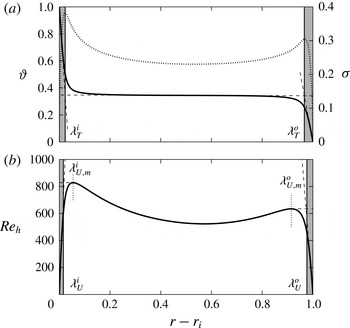
exhibits sharp local maxima close to the walls. The radial distance separating those peaks from the corresponding nearest boundary can be used to define the thermal boundary layer thicknesses (e.g. Tilgner Reference Tilgner1996; King, Stellmach & Buffett Reference King, Stellmach and Buffett2013). Figure 2(a) shows that both definitions of
 ${\it\lambda}_{T}$
actually yield nearly indistinguishable boundary layer thicknesses. We therefore adopt the slope method to define the thermal boundary layers.
(a) Radial profiles of the time and horizontally averaged mean temperature
 ${\it\vartheta}(r)$
(solid black line) and the temperature variance
 ${\it\sigma}$
(dotted black line). The thermal boundary layers
 ${\it\lambda}_{T}^{i}$
and
 ${\it\lambda}_{T}^{o}$
are highlighted by the grey shaded area. They are defined as the depths where the linear fit to
 ${\it\vartheta}(r)$
near the top (bottom) crosses the linear fit to the temperature profile at mid-depth (dashed black lines). (b) Radial profiles of the time and horizontally averaged horizontal velocity
 $\mathit{Re}_{h}(r)$
. The viscous boundary layers are either defined by the local maxima of
 $\mathit{Re}_{h}$
(black dotted lines,
 ${\it\lambda}_{U,m}^{i}$
,
 ${\it\lambda}_{U,m}^{o}$
) or by the intersection of the linear fit to
 $\mathit{Re}_{h}$
near the inner (outer) boundary with the tangent to the local maxima (dashed black lines). This second definition is highlighted by a grey shaded area (
 ${\it\lambda}_{U}^{i}$
,
 ${\it\lambda}_{U}^{o}$
). These profiles have been obtained from a numerical model with
 $\mathit{Ra}=10^{7}$
,
 ${\it\eta}=0.6$
and
 $g=(r_{o}/r)^{2}$
.

There are also several ways to define the viscous boundary layers. Figure 2(b) shows the vertical profile of the root-mean-square horizontal velocity
 $\mathit{Re}_{h}$
. This profile exhibits strong increases close to the boundaries that are accompanied by well-defined peaks. Following Tilgner (Reference Tilgner1996) and Kerr & Herring (Reference Kerr and Herring2000), the first way to define the kinematic boundary layer is thus to measure the distance between the walls and these local maxima. This commonly used definition gives
 ${\it\lambda}_{U,m}^{i}$
(
 ${\it\lambda}_{U,m}^{o}$
) for the inner (outer) spherical boundary. Another possible method to estimate the viscous boundary layer follows a similar strategy as the slope method that we adopted for the thermal boundary layers (Breuer et al.
Reference Breuer, Wessling, Schmalzl and Hansen2004).
 ${\it\lambda}_{U}^{i}$
(
 ${\it\lambda}_{U}^{o}$
) is defined as the distance from the inner (outer) wall where the linear fit to
 $\mathit{Re}_{h}$
near the inner (outer) boundary intersects the horizontal line passing through the maximum horizontal velocity.
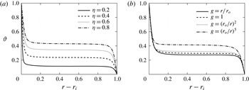
(a)
 ${\it\vartheta}(r)$
for different radius ratios
 ${\it\eta}$
with a gravity
 $g=(r_{o}/r)^{2}$
. These models have approximately the same Nusselt number
 $12<Nu<14$
. (b)
 ${\it\vartheta}(r)$
for different gravity profiles with a fixed radius ratio
 ${\it\eta}=0.6$
. These models have approximately the same Nusselt number
 $10<Nu<11$
.

Figure 2(b) reveals that these two definitions lead to very distinct viscous boundary layer thicknesses. In particular, the definition based on the position of the local maxima of
 $\mathit{Re}_{h}$
yields much thicker boundary layers than the tangent intersection method, i.e.
 ${\it\lambda}_{U,m}^{i,o}>{\it\lambda}_{U}^{i,o}$
. The discrepancies of these two definitions are further discussed in § 4.
3.2. Asymmetric thermal boundary layers and mean bulk temperature
Figure 2 also reveals a pronounced asymmetry in the mean temperature profiles with a much larger temperature drop at the inner boundary than at the outer boundary. As a consequence, the mean temperature of the spherical shell
 $T_{m}=(1/V)\int _{V}T\,\text{d}V$
is far below
 ${\rm\Delta}T/2$
. Determining how the mean temperature depends on the radius ratio
 ${\it\eta}$
has been an ongoing open question in mantle convection studies with infinite Prandtl number (e.g. Bercovici et al.
Reference Bercovici, Schubert, Glatzmaier and Zebib1989; Jarvis Reference Jarvis1993; Vangelov & Jarvis Reference Vangelov and Jarvis1994; Jarvis et al.
Reference Jarvis, Glatzmaier and Vangelov1995; Sotin & Labrosse Reference Sotin and Labrosse1999; Shahnas et al.
Reference Shahnas, Lowman, Jarvis and Bunge2008; Deschamps et al.
Reference Deschamps, Tackley and Nakagawa2010; O’Farrell et al.
Reference O’Farrell, Lowman and Bunge2013). To analyse this issue in numerical models with
 $\mathit{Pr}=1$
, we have performed a systematic parameter study varying both the radius ratio of the spherical shell
 ${\it\eta}$
and the gravity profile
 $g(r)$
(see table 2). Figure 3 shows some selected radial profiles of the mean temperature
 ${\it\vartheta}$
for various radius ratios (a) and gravity profiles (b) for cases with similar
 $\mathit{Nu}$
. For small values of
 ${\it\eta}$
, the large difference between the inner and the outer surfaces lead to a strong asymmetry in the temperature distribution: nearly 90 % of the total temperature drop occurs at the inner boundary when
 ${\it\eta}=0.2$
. In thinner spherical shells, the mean temperature gradually approaches a more symmetric distribution to finally reach
 $T_{m}=0.5$
when
 ${\it\eta}\rightarrow 1$
(no curvature). Figure 3(b) also reveals that a change in the gravity profile has a direct impact on the mean temperature profile. This shows that both the shell geometry and the radial distribution of buoyancy affect the temperature of the fluid bulk in RB convection in spherical shells.
To analytically access the asymmetries in thickness and temperature drop observed in figure 3, we first assume that heat is purely transported by conduction in the thin thermal boundary layers. Heat flux conservation through spherical surfaces (2.10) then yields
 $$\begin{eqnarray}\frac{{\rm\Delta}T^{o}}{{\it\lambda}_{T}^{o}}={\it\eta}^{2}\frac{{\rm\Delta}T^{i}}{{\it\lambda}_{T}^{i}},\end{eqnarray}$$
where the thermal boundary layers are assumed to correspond to a linear conduction profile with a temperature drop
 ${\rm\Delta}T^{i}$
(
 ${\rm\Delta}T^{o}$
) over a thickness
 ${\it\lambda}_{T}^{i}$
(
 ${\it\lambda}_{T}^{o}$
). As shown in figures 2 and 3, the fluid bulk is isothermal and forms the majority of the fluid by volume. We can thus further assume that the temperature drops occur only in the thin boundary layers, which leads to
 $$\begin{eqnarray}{\rm\Delta}T^{o}+{\rm\Delta}T^{i}=1.\end{eqnarray}$$
Equations (3.2) and (3.3) are nevertheless not sufficient to determine the three unknowns
 ${\rm\Delta}T^{i}$
,
 ${\rm\Delta}T^{o}$
,
 ${\it\lambda}_{T}^{o}/{\it\lambda}_{T}^{i}$
and an additional physical assumption is required.
A hypothesis frequently used in mantle convection models with infinite Prandtl number in a spherical geometry (Jarvis Reference Jarvis1993; Vangelov & Jarvis Reference Vangelov and Jarvis1994) is to further assume that both thermal boundary layers are marginally stable such that the local boundary layer Rayleigh numbers
 $\mathit{Ra}_{{\it\lambda}}^{i}$
and
 $\mathit{Ra}_{{\it\lambda}}^{o}$
are equal:
 $$\begin{eqnarray}\mathit{Ra}_{{\it\lambda}}^{i}=\mathit{Ra}_{{\it\lambda}}^{o}\,\rightarrow \,\frac{{\it\alpha}g_{i}{\rm\Delta}T^{i}{{\it\lambda}_{T}^{i}}^{3}}{{\it\nu}{\it\kappa}}=\frac{{\it\alpha}g_{o}{\rm\Delta}T^{o}{{\it\lambda}_{T}^{o}}^{3}}{{\it\nu}{\it\kappa}}.\end{eqnarray}$$
This means that both thermal boundary layers adjust their thickness and temperature drop to yield
 $\mathit{Ra}_{{\it\lambda}}^{i}\sim \mathit{Ra}_{{\it\lambda}}^{o}\sim \mathit{Ra}_{c}\simeq 1000$
(e.g. Malkus Reference Malkus1954). The temperature drops at both boundaries and the ratio of the thermal boundary layer thicknesses can then be derived using (3.2) and (3.3)
 $$\begin{eqnarray}{\rm\Delta}T^{i}=\frac{1}{1+{\it\eta}^{3/2}\,{\it\chi}_{g}^{1/4}},\quad {\rm\Delta}T^{o}\simeq T_{m}=\frac{{\it\eta}^{3/2}\,{\it\chi}_{g}^{1/4}}{1+{\it\eta}^{3/2}\,{\it\chi}_{g}^{1/4}},\quad \frac{{\it\lambda}_{T}^{o}}{{\it\lambda}_{T}^{i}}=\frac{{\it\chi}_{g}^{1/4}}{{\it\eta}^{1/2}},\end{eqnarray}$$
where
 $$\begin{eqnarray}{\it\chi}_{g}=\frac{g(r_{i})}{g(r_{o})},\end{eqnarray}$$
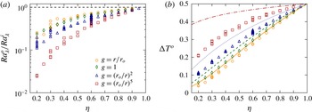
is the ratio of the gravitational acceleration between the inner and the outer boundaries. Figure 4(a) reveals that the marginal stability hypothesis is not fulfilled when different radius ratios and gravity profiles are considered. This is particularly obvious for small radius ratios where
 $\mathit{Ra}_{{\it\lambda}}^{o}$
is more than 10 times larger than
 $\mathit{Ra}_{{\it\lambda}}^{i}$
. This discrepancy tends to vanish when
 ${\it\eta}\rightarrow 1$
, where curvature and gravity variations become unimportant. As a consequence, there is a significant mismatch between the predicted mean bulk temperature from (3.5) and the actual values (figure 4
b). Deschamps et al. (Reference Deschamps, Tackley and Nakagawa2010) also reported a similar deviation from (3.5) in their spherical shell models with infinite Prandtl number. They suggest that assuming instead
 $\mathit{Ra}_{{\it\lambda}}^{o}/\mathit{Ra}_{{\it\lambda}}^{i}\sim {\it\eta}^{2}$
might help to improve the agreement with the data. This however cannot account for the additional dependence on the gravity profile visible in figure 4. We finally note that
 $\mathit{Ra}_{{\it\lambda}}<400$
for the database of numerical simulations explored here, which suggests that the thermal boundary layers are stable in all our simulations.
(a) Ratio of boundary layer Rayleigh numbers (3.4) for various radius ratios and gravity profiles. The horizontal dashed line corresponds to the hypothetical identity
 $\mathit{Ra}_{{\it\lambda}}^{i}=\mathit{Ra}_{{\it\lambda}}^{o}$
. (b) Temperature drop at the outer boundary layer. The lines correspond to the theoretical prediction given in (3.5).

Alternatively Wu & Libchaber (Reference Wu and Libchaber1991) and Zhang, Childress & Libchaber (Reference Zhang, Childress and Libchaber1997) proposed that the thermal boundary layers adapt their thicknesses such that the mean hot and cold temperature fluctuations at mid-depth are equal. Their experiments with Helium indeed revealed that the statistical distribution of the temperature at mid-depth was symmetrical. They further assumed that the thermal fluctuations at mid-depth can be identified with the boundary layer temperature scales
 ${\it\theta}^{i}=({\it\nu}{\it\kappa})/({\it\alpha}g_{i}{{\it\lambda}_{T}^{i}}^{3})$
and
 ${\it\theta}^{o}=({\it\nu}{\it\kappa})/({\it\alpha}g_{o}{{\it\lambda}_{T}^{o}}^{3})$
, which characterise the temperature scale of the thermal boundary layers in a different way than the relative temperature drops
 ${\rm\Delta}T^{i}$
and
 ${\rm\Delta}T^{o}$
. This second hypothesis yields
 $$\begin{eqnarray}{\it\theta}^{i}={\it\theta}^{o}\,\rightarrow \,\frac{{\it\nu}{\it\kappa}}{{\it\alpha}g_{i}{{\it\lambda}_{T}^{i}}^{3}}=\frac{{\it\nu}{\it\kappa}}{{\it\alpha}g_{o}{{\it\lambda}_{T}^{o}}^{3}},\end{eqnarray}$$
and the corresponding temperature drops and boundary layer thicknesses ratio
 $$\begin{eqnarray}{\rm\Delta}T^{i}=\frac{1}{1+{\it\eta}^{2}\,{\it\chi}_{g}^{1/3}},\quad {\rm\Delta}T^{o}=T_{m}=\frac{{\it\eta}^{2}\,{\it\chi}_{g}^{1/3}}{1+{\it\eta}^{2}\,{\it\chi}_{g}^{1/3}},\quad \frac{{\it\lambda}_{T}^{o}}{{\it\lambda}_{T}^{i}}={\it\chi}_{g}^{1/3}.\end{eqnarray}$$
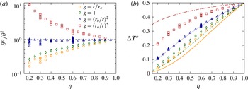
Figure 5(a) shows
 ${\it\theta}^{o}/{\it\theta}^{i}$
for different radius ratios and gravity profiles, while figure 5(b) shows a comparison between the predicted mean bulk temperature and the actual values. Besides the cases with
 $g=(r_{o}/r)^{2}$
, which are in relatively good agreement with the predicted scalings, the identity of the boundary layer temperature scale is in general not fulfilled for the other gravity profiles. The actual mean bulk temperature is thus poorly described by (3.8). We note that previous findings by Ahlers et al. (Reference Ahlers, Brown, Fontenele Araujo, Funfschilling, Grossmann and Lohse2006) already reported that the theory by Wu & Libchaber’s does also not hold when the transport properties depend on temperature (i.e. non-Oberbeck–Boussinesq convection).
(a) Ratio of boundary layer temperature scales (3.7) for various radius ratios and gravity profiles. The horizontal dashed line corresponds to the hypothetical identity
 ${\it\theta}^{i}={\it\theta}^{o}$
. (b) Temperature drop at the outer boundary layer. The lines correspond to the theoretical prediction given in (3.8).

3.3. Conservation of the average plume density in spherical shells
As demonstrated in the previous section, none of the hypotheses classically employed accurately account for the temperature drops and the boundary layer asymmetry observed in spherical shells. We must therefore find a dynamical quantity that could possibly be identified between the two boundary layers.
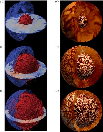
Figure 6 shows visualisations of the thermal boundary layers for three selected numerical models with different radius ratios and gravity profiles. The isocontours displayed in (a–c) reveal the intricate plume structure. Long and thin sheet-like structures form the main network of plumes. During their migration along the spherical surfaces, these sheet-like plumes can collide and convolute with each other to give rise to mushroom-type plumes (see Zhou & Xia Reference Zhou and Xia2010b
; Chillà & Schumacher Reference Chillà and Schumacher2012). During this morphological evolution, mushroom-type plumes acquire a strong radial vorticity component. These mushroom-type plumes are particularly visible at the connection points of the sheet plumes network at the inner thermal boundary layer (red isosurface in figure 6
a–c). Figure 6(d–f) shows the corresponding equatorial and radial cuts of the temperature fluctuation
 $T^{\prime }=T-{\it\vartheta}$
. These panels further highlight the plume asymmetry between the inner and the outer thermal boundary layers. For instance, the case with
 ${\it\eta}=0.3$
and
 $g=(r_{o}/r)^{5}$
(a,d) features an outer boundary layer approximately 4.5 times thicker than the inner one. Accordingly, the mushroom-type plumes that depart from the outer boundary layer are significantly thicker than the ones emitted from the inner boundary. This discrepancy tends to vanish in the thin shell case (
 ${\it\eta}=0.8$
, c,f) in which curvature and gravity variations play a less significant role (
 ${\it\lambda}_{T}^{o}/{\it\lambda}_{T}^{i}\simeq 1.02$
in that case).
(a–c) Isosurfaces and equatorial cut of the temperature for three numerical models: hot at the inner thermal boundary layer
 $T(r=r_{i}+{\it\lambda}_{T}^{i})$
in red, cold at the outer thermal boundary layer
 $T(r=r_{o}-{\it\lambda}_{T}^{o})$
in blue. (d–f) Meridional cuts and surfaces of the temperature fluctuations
 $T^{\prime }$
. The inner (outer) surface corresponds to the location of the inner (outer) thermal boundary layers. Color levels range from
 $-$
0.2 (black) to 0.2 (white). (a,d) Correspond to a model with
 $\mathit{Ra}=3\times 10^{6},\,{\it\eta}=0.3$
and
 $g=(r_{o}/r)^{5}$
. (b,e) Correspond to a model with
 $\mathit{Ra}=10^{8},\,{\it\eta}=0.6$
and
 $g=(r_{o}/r)^{2}$
. (c,f) Correspond to a model with
 $\mathit{Ra}=4\times 10^{7},\,{\it\eta}=0.8$
and
 $g=r/r_{o}$
.

Puthenveettil & Arakeri (Reference Puthenveettil and Arakeri2005) and Zhou & Xia (Reference Zhou and Xia2010b ) performed a statistical analysis of the geometrical properties of thermal plumes in experimental RB convection. By tracking a large number of plumes, their analysis revealed that both the plume separation and the width of the sheet-like plumes follow a log-normal probability density function (PDF).
To further assess how the average plume properties of the inner and outer thermal boundary layers compare with each other in a spherical geometry, we adopt a simpler strategy by only focusing on the statistics of the plume density. The plume density per surface unit at a given radius
 $r$
is expressed by
 $$\begin{eqnarray}{\it\rho}_{p}\sim {\displaystyle \frac{N}{4{\rm\pi}r^{2}}},\end{eqnarray}$$
where
 $N$
is the number of plumes, approximated here by the ratio of the spherical surface area to the mean inter-plume area
 $\bar{\mathscr{S}}$
:
 $$\begin{eqnarray}N\sim \frac{4{\rm\pi}r^{2}}{\bar{\mathscr{S}}}.\end{eqnarray}$$
This inter-plume area
 $\bar{\mathscr{S}}$
can be further related to the average plume separation
 $\bar{\ell }$
via
 $\bar{\mathscr{S}}\sim ({\rm\pi}/4)\,\bar{\ell }^{2}$
.
An accurate evaluation of the inter-plume area for each thermal boundary layer however requires the extraction of the plumes from the background fluid. Most of the criteria employed to determine the location of the plume boundaries are based on thresholds of certain physical quantities (see Shishkina & Wagner Reference Shishkina and Wagner2008, for a review of the different plume extraction techniques). This encompasses threshold values on the temperature fluctuations
 $T^{\prime }$
(Zhou & Xia Reference Zhou and Xia2002), on the vertical velocity
 $u_{r}$
(Ching et al.
Reference Ching, Guo, Shang, Tong and Xia2004) or on the thermal dissipation rate
 ${\it\epsilon}_{T}$
(Shishkina & Wagner Reference Shishkina and Wagner2005). The choice of the threshold value however remains an open problem. Alternatively, Vipin & Puthenveettil (Reference Vipin and Puthenveettil2013) show that the sign of the horizontal divergence of the velocity
 $\boldsymbol{{\rm\nabla}}_{H}\boldsymbol{\cdot }\boldsymbol{u}$
might provide a simple and threshold-free criterion to separate the plumes from the background fluid
 $$\begin{eqnarray}\boldsymbol{{\rm\nabla}}_{H}\boldsymbol{\cdot }\boldsymbol{u}=\frac{1}{r\sin {\it\theta}}\frac{\partial }{\partial {\it\theta}}(\sin {\it\theta}\,u_{{\it\theta}})+\frac{1}{r\sin {\it\theta}}\frac{\partial u_{{\it\phi}}}{\partial {\it\phi}}=-\frac{1}{r^{2}}\frac{\partial }{\partial r}(r^{2}\,u_{r}).\end{eqnarray}$$
Fluid regions with
 $\boldsymbol{{\rm\nabla}}_{H}\boldsymbol{\cdot }\boldsymbol{u}<0$
indeed correspond to local regions of positive vertical acceleration, expected inside the plumes, while the fluid regions with
 $\boldsymbol{{\rm\nabla}}_{H}\boldsymbol{\cdot }\boldsymbol{u}>0$
characterise the inter-plume area.
To analyse the statistics of
 $\mathscr{S}$
, we thus consider here several criteria based either on a threshold value of the temperature fluctuations or on the sign of the horizontal divergence. This means that a given inter-plume area at the inner (outer) thermal boundary layer is either defined as an enclosed region surrounded by hot (cold) sheet-like plumes carrying a temperature perturbation
 $|T^{\prime }|>t$
; or by an enclosed region with
 $\boldsymbol{{\rm\nabla}}_{H}\boldsymbol{\cdot }\boldsymbol{u}>0$
. To further estimate the possible impact of the chosen threshold value on
 $\mathscr{S}$
, we vary
 $t$
between
 ${\it\sigma}/4$
and
 ${\it\sigma}$
. This yields
 $$\begin{eqnarray}\mathscr{S}(r)\equiv r^{2}\oint _{\mathscr{T}}\sin {\it\theta}\,\text{d}{\it\theta}\,\text{d}{\it\phi},\end{eqnarray}$$
where the physical criterion
 $\mathscr{T}_{i}$
(
 $\mathscr{T}_{o}$
) to extract the plume boundaries at the inner (outer) boundary layer is given by
 $$\begin{eqnarray}\left.\begin{array}{@{}c@{}}\mathscr{T}_{i}=\left\{\begin{array}{@{}ll@{}}T^{\prime }(r_{{\it\lambda}}^{i},{\it\theta},{\it\phi})\leqslant t,\quad & t\in [{\it\sigma}(r_{{\it\lambda}}^{i}),{\it\sigma}(r_{{\it\lambda}}^{i}/2),{\it\sigma}(r_{{\it\lambda}}^{i}/4)],\\ \boldsymbol{{\rm\nabla}}_{H}\boldsymbol{\cdot }\boldsymbol{u}\geqslant 0,\quad & \end{array}\right.\\ \mathscr{T}_{o}=\left\{\begin{array}{@{}ll@{}}T^{\prime }(r_{{\it\lambda}}^{o},{\it\theta},{\it\phi})\geqslant t,\quad & t\in [{\it\sigma}(r_{{\it\lambda}}^{i}),{\it\sigma}(r_{{\it\lambda}}^{i}/2),{\it\sigma}(r_{{\it\lambda}}^{i}/4)],\\ \boldsymbol{{\rm\nabla}}_{H}\boldsymbol{\cdot }\boldsymbol{u}\geqslant 0,\quad & \end{array}\right.\end{array}\right\}\end{eqnarray}$$
where
 $r_{{\it\lambda}}^{i}=r_{i}+{\it\lambda}_{T}^{i}$
(
 $r_{{\it\lambda}}^{o}=r_{o}-{\it\lambda}_{T}^{o}$
) for the inner (outer) thermal boundary layer.
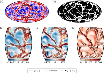
Figure 7 shows an example of such a characterisation procedure for the inner thermal boundary layer of a numerical model with
 $\mathit{Ra}=10^{6}$
,
 ${\it\eta}=0.6$
,
 $g=(r_{o}/r)^{2}$
. (b) Illustrates a plume extraction process when using
 $|T^{\prime }|>{\it\sigma}/2$
to determine the location of the plumes: the black area correspond to the inter-plume spacing while the white area correspond to the complementary plume network location. The fainter emerging sheet-like plumes are filtered out and only the remaining ‘skeleton’ of the plume network is selected by this extraction process. The choice of
 ${\it\sigma}/2$
is however arbitrary and can influence the evaluation of the number of plumes. The insets displayed in (c–e) illustrate the sensitivity of the plume extraction process on the criterion employed to detect the plumes. In particular, using the threshold based on the largest temperature fluctuations
 $|T^{\prime }|>{\it\sigma}$
can lead to the fragmentation of the detected plume lanes into several isolated smaller regions. As a consequence, several neighbouring inter-plume areas may be artificially connected when using this criterion. In contrast, using the sign of the horizontal divergence to estimate the plumes location yields much broader sheet-like plumes. As visible in (e), the plume boundaries frequently correspond to local maxima of the thermal dissipation rate
 ${\it\epsilon}_{T}$
(Shishkina & Wagner Reference Shishkina and Wagner2008).
(a) Temperature fluctuation at the inner thermal boundary layer
 $T^{\prime }(r=r_{i}+{\it\lambda}_{T}^{i})$
displayed in a Hammer projection for a case with
 $\mathit{Ra}=10^{6}$
,
 ${\it\eta}=0.6$
,
 $g=(r_{o}/r)^{2}$
. (b) Corresponding binarised extraction of the plumes boundaries using (3.12) and
 $T^{\prime }\leqslant {\it\sigma}/2$
to define the inter-plume area. Zoomed-in contour of the temperature fluctuation
 $T^{\prime }$
(c), the horizontal divergence
 $-\boldsymbol{{\rm\nabla}}_{H}\boldsymbol{\cdot }\boldsymbol{u}$
(d) and the thermal dissipation rate
 ${\it\epsilon}_{T}$
(e). The three black contour lines in (c–e) correspond to several criteria to extract the plume boundaries (3.13).

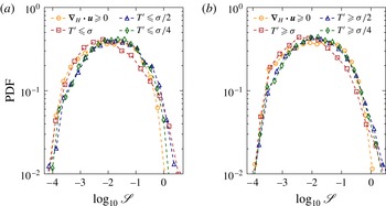
For each criterion given in (3.13), we then calculate the area of each bounded black surface visible in figure 7(b) to construct the statistical distribution of the inter-plume area for both thermal boundary layers. Figure 8 compares the resulting PDFs obtained by combining several snapshots for a numerical model with
 $\mathit{Ra}=4\times 10^{7}$
,
 ${\it\eta}=0.8$
and
 $g=r/r_{o}$
. Besides the criterion
 $|T^{\prime }|>{\it\sigma}$
which yields PDFs that are slightly shifted towards smaller inter-plume spacing areas, the statistical distributions are found to be relatively insensitive to the detection criterion (3.13). We therefore restrict the following comparison to the criterion
 $|T^{\prime }|>{\it\sigma}/2$
only.
Probability density functions (PDFs) of the dimensionless inter-plume area
 $\mathscr{S}$
at the inner
 $r=r_{i}+{\it\lambda}_{T}^{i}$
(a) and at the outer
 $r=r_{o}-{\it\lambda}_{T}^{o}$
(b) thermal boundary layers using different criteria to extract the plumes (3.13) for a model with
 $\mathit{Ra}=4\times 10^{7}$
,
 ${\it\eta}=0.8$
and
 $g=r/r_{o}$
.

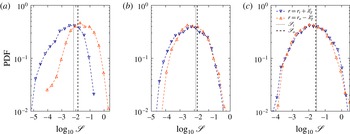
Figure 9 shows the PDFs for the three numerical models of figure 6. For the two cases with
 ${\it\eta}=0.6$
and
 ${\it\eta}=0.8$
(b,c), the statistical distributions for both thermal boundary layers nearly overlap. This means that the inter-plume area is similar at both spherical shell surfaces. In contrast, for the case with
 ${\it\eta}=0.3$
(a), the two PDFs are offset relative to each other. However, the peaks of the distributions remain relatively close, meaning that once again the inner and the outer thermal boundary layers share a similar average inter-plume area. Puthenveettil & Arakeri (Reference Puthenveettil and Arakeri2005) and Zhou & Xia (Reference Zhou and Xia2010b
) demonstrated that the thermal plume statistics in turbulent RB convection follow a log-normal distribution (see also Shishkina & Wagner Reference Shishkina and Wagner2008; Puthenveettil et al.
Reference Puthenveettil, Gunasegarane, Agrawal, Schmeling, Bosbach and Arakeri2011). The large number of plumes in the cases with
 ${\it\eta}=0.6$
and
 ${\it\eta}=0.8$
(figure 6
b,c) would allow a characterisation of the nature of the statistical distributions. However, this would be much more difficult in the
 ${\it\eta}=0.3$
case (figure 6
a) in which the plume density is significantly weaker. As a consequence, no further attempt has been made to characterise the exact nature of the PDFs visible in figure 9, although the universality of the log-normal statistics reported by Puthenveettil & Arakeri (Reference Puthenveettil and Arakeri2005) and Zhou & Xia (Reference Zhou and Xia2010b
) likely indicates that the same statistical distribution should hold here too.
PDF of the dimensionless inter-plume area
 $\mathscr{S}$
at the outer (orange upward triangles) and at the inner (blue downward triangles) thermal boundary layers using
 $|T^{\prime }|>{\it\sigma}/2$
to extract plumes. (a) Corresponds to a numerical model with
 $\mathit{Ra}=3\times 10^{6},\,{\it\eta}=0.3$
and
 $g=(r_{o}/r)^{5}$
. (b) Corresponds to a model with
 $\mathit{Ra}=10^{8},\,{\it\eta}=0.6$
and
 $g=(r_{o}/r)^{2}$
. (c) Corresponds to a model with
 $\mathit{Ra}=4\times 10^{7},\,{\it\eta}=0.8$
and
 $g=r/r_{o}$
. The two vertical lines correspond to the predicted values of the mean inter-plume area
 $\bar{\mathscr{S}}$
derived from (3.16) for both thermal boundary layers.

The inter-plume area statistics therefore reveal that the inner and the outer thermal boundary layers exhibit a similar average plume density, independently of the spherical shell geometry and the gravity profile. Assuming
 ${\it\rho}_{p}^{o}\simeq {\it\rho}_{p}^{i}$
would allow us to close the system of (3.2)–(3.3) and thus finally estimate
 ${\rm\Delta}T^{i}$
,
 ${\rm\Delta}T^{o}$
and
 ${\it\lambda}_{T}^{o}/{\it\lambda}_{T}^{i}$
. This however requires us to determine an analytical expression of the average inter-plume area
 $\bar{\mathscr{S}}$
or equivalently of the mean plume separation
 $\bar{\ell }$
that depends on the boundary layer thickness and the temperature drop.
Using the boundary layer equations for natural convection (Rotem & Claassen Reference Rotem and Claassen1969), Puthenveettil et al. (Reference Puthenveettil, Gunasegarane, Agrawal, Schmeling, Bosbach and Arakeri2011) demonstrated that the thermal boundary layer thickness follows
 $$\begin{eqnarray}{\it\lambda}_{T}^{i,o}(x)\sim \frac{x}{(\mathit{Ra}_{x}^{i,o})^{1/5}},\end{eqnarray}$$
where
 $x$
is the distance along the horizontal direction and
 $\mathit{Ra}_{x}^{i,o}={\it\alpha}g{\rm\Delta}T^{i,o}x^{3}/{\it\nu}{\it\kappa}$
is a Rayleigh number based on the length scale
 $x$
and on the boundary layer temperature jumps
 ${\rm\Delta}T^{i,o}$
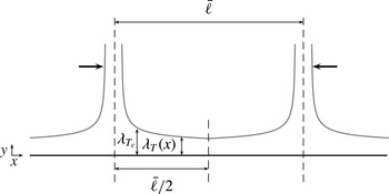
. As shown on figure 10, using
 $x=\bar{\ell }/2$
(Puthenveettil & Arakeri Reference Puthenveettil and Arakeri2005; Puthenveettil et al.
Reference Puthenveettil, Gunasegarane, Agrawal, Schmeling, Bosbach and Arakeri2011) then allows the following relation for the average plume spacing to be established
 $$\begin{eqnarray}\frac{{\it\lambda}_{T}}{\bar{\ell }}\sim \frac{1}{\mathit{Ra}_{\ell }^{1/5}}\end{eqnarray}$$
which yields
 $$\begin{eqnarray}\bar{\ell }_{i}\sim \sqrt{\frac{{\it\alpha}g_{i}{\rm\Delta}T^{i}{{\it\lambda}_{T}^{i}}^{5}}{{\it\nu}{\it\kappa}}},\quad \bar{\ell }_{o}\sim \sqrt{\frac{{\it\alpha}g_{o}{\rm\Delta}T^{o}{{\it\lambda}_{T}^{o}}^{5}}{{\it\nu}{\it\kappa}}},\end{eqnarray}$$
for both thermal boundary layers. We note that an equivalent expression for the average plume spacing can be derived from a simple mechanical description of the equilibrium between production and coalescence of plumes in each boundary layer (see Parmentier & Sotin Reference Parmentier and Sotin2000; King et al. Reference King, Stellmach and Buffett2013).
Schematic showing two adjacent plumes separated by a distance
 $\bar{\ell }$
. The thick black arrows indicate the direction of merging of the two plumes.

Equation (3.16) is however expected to be valid only at the scaling level. The vertical lines in figure 9 therefore correspond to the estimated average inter-plume area for both thermal boundary layers using (3.16) and
 $\bar{\mathscr{S}}_{i,o}=0.3\,\bar{\ell }_{i,o}^{2}$
. The predicted average inter-plume area is in good agreement with the peaks of the statistical distributions for the three cases discussed here. The expression (3.16) therefore provides a reasonable estimate of the average plume separation (Puthenveettil & Arakeri Reference Puthenveettil and Arakeri2005; Puthenveettil et al.
Reference Puthenveettil, Gunasegarane, Agrawal, Schmeling, Bosbach and Arakeri2011; Gunasegarane & Puthenveettil Reference Gunasegarane and Puthenveettil2014). The comparable observed plume density at both thermal boundary layers thus yields
 $$\begin{eqnarray}{\it\rho}_{p}^{i}={\it\rho}_{p}^{o}\,\rightarrow \,\frac{{\it\alpha}g_{i}{\rm\Delta}T^{i}{{\it\lambda}_{T}^{i}}^{5}}{{\it\nu}{\it\kappa}}=\frac{{\it\alpha}g_{o}{\rm\Delta}T^{o}{{\it\lambda}_{T}^{o}}^{5}}{{\it\nu}{\it\kappa}}.\end{eqnarray}$$
Using (3.2) and (3.3) then allows us to finally estimate the temperature jumps and the ratio of the thermal boundary layer thicknesses in our dimensionless units:
 $$\begin{eqnarray}{\rm\Delta}T^{i}=\frac{1}{1+{\it\eta}^{5/3}\,{\it\chi}_{g}^{1/6}},\quad {\rm\Delta}T^{o}=T_{m}=\frac{{\it\eta}^{5/3}\,{\it\chi}_{g}^{1/6}}{1+{\it\eta}^{5/3}\,{\it\chi}_{g}^{1/6}},\quad \frac{{\it\lambda}_{T}^{o}}{{\it\lambda}_{T}^{i}}=\frac{{\it\chi}_{g}^{1/6}}{{\it\eta}^{1/3}}.\end{eqnarray}$$
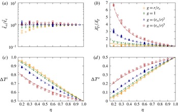
Figure 11 shows the ratios
 $\bar{\ell }_{o}/\bar{\ell }_{i}$
,
 ${\it\lambda}_{T}^{o}/{\it\lambda}_{T}^{i}$
and the temperature jumps
 ${\rm\Delta}T^{i}$
and
 ${\rm\Delta}T^{o}$
. In contrast to the previous criteria, either coming from the marginal stability of the boundary layer ((3.5), figure 4) or from the identity of the temperature fluctuations at mid-shell ((3.18), figure 5), the ratio of the average plume separation
 $\bar{\ell }_{o}/\bar{\ell }_{i}$
now falls much closer to the unity line. Some deviations are nevertheless still visible for spherical shells with
 ${\it\eta}\leqslant 0.4$
and
 $g=r/r_{o}$
(orange circles). The comparable average plume density between both boundary layers allows us to accurately predict the asymmetry of the thermal boundary layers
 ${\it\lambda}_{T}^{o}/{\it\lambda}_{T}^{i}$
and the corresponding temperature drops for the vast majority of the numerical cases explored here (solid lines in b–d).
(a) Ratio of the thermal plume separation estimated by (3.16) for various radius ratios and gravity profiles. The horizontal dashed line corresponds to the identity of the average plume separation between both thermal boundary layers, i.e.
 $\bar{\ell }^{i}=\bar{\ell }^{o}$
. (b) Ratio of thermal boundary layer thicknesses. (c) Temperature drop at the inner boundary layer. (d) Temperature drop at the outer boundary layer. The lines in (b–d) correspond to the theoretical prediction given in (3.18).

As we consider a fluid with
 $\mathit{Pr}=1$
, the viscous boundary layers should show a comparable degree of asymmetry as the thermal boundary layers. Equation (3.18) thus implies
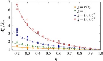
 $$\begin{eqnarray}\frac{{\it\lambda}_{U}^{o}}{{\it\lambda}_{U}^{i}}=\frac{{\it\lambda}_{T}^{o}}{{\it\lambda}_{T}^{i}}=\frac{{\it\chi}_{g}^{1/6}}{{\it\eta}^{1/3}}.\end{eqnarray}$$
Figure 12 shows the ratio of the viscous boundary layer thicknesses for the different setups explored in this study. The observed asymmetry between the two spherical shell surfaces is in a good agreement with (3.19) (solid black lines).
Ratio of the viscous boundary layer thicknesses for various aspect ratios and gravity profiles. The lines correspond to the theoretical prediction given in (3.19).

3.4. Thermal boundary layer scalings
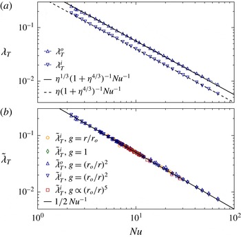
Using (3.18) and the definition of the Nusselt number (2.10), we can derive the following scaling relations for the thermal boundary layer thicknesses:
 $$\begin{eqnarray}{\it\lambda}_{T}^{i}=\frac{{\it\eta}}{1+{\it\eta}^{5/3}\,{\it\chi}_{g}^{1/6}}\,\frac{1}{\mathit{Nu}},\quad {\it\lambda}_{T}^{o}=\frac{{\it\eta}^{2/3}{\it\chi}_{g}^{1/6}}{1+{\it\eta}^{5/3}\,{\it\chi}_{g}^{1/6}}\,\frac{1}{\mathit{Nu}}.\end{eqnarray}$$
Figure 13(a) demonstrates that the boundary layer thicknesses for the numerical simulations of table 1 (
 $g=(r_{o}/r)^{2}$
and
 ${\it\eta}=0.6$
) are indeed in close agreement with the theoretical predictions. To further check this scaling for other spherical shell configurations, we introduce the following normalisation of the thermal boundary layer thicknesses
 $$\begin{eqnarray}\tilde{{\it\lambda}}_{T}^{i}=\frac{1}{2}\,\frac{1+{\it\eta}^{5/3}\,{\it\chi}_{g}^{1/6}}{{\it\eta}}{\it\lambda}_{T}^{i},\quad \tilde{{\it\lambda}}_{T}^{o}=\frac{1}{2}\,\frac{1+{\it\eta}^{5/3}\,{\it\chi}_{g}^{1/6}}{{\it\eta}^{2/3}\,{\it\chi}_{g}^{1/6}}{\it\lambda}_{T}^{o}.\end{eqnarray}$$
This allows us to derive a unified scaling that does not depend on the choice of the gravity profile or on the spherical shell geometry
 $$\begin{eqnarray}\tilde{{\it\lambda}}_{T}=\tilde{{\it\lambda}}_{T}^{i}=\tilde{{\it\lambda}}_{T}^{o}=\frac{1}{2\,\mathit{Nu}}.\end{eqnarray}$$
Figure 13(b) shows this normalised boundary layer thickness for the different spherical shell configurations explored here. Despite the variety of the physical set-ups, the normalised boundary layer thicknesses are in good agreement with the predicted behaviour.
(a) Thermal boundary layer thicknesses at the outer boundary (
 ${\it\lambda}_{T}^{i}$
) and at the inner boundary (
 ${\it\lambda}_{T}^{o}$
) as a function of the Nusselt number for the cases of table 1. The two lines correspond to the theoretical predictions from (3.20). (b) Normalised boundary layer thicknesses as a function of the Nusselt number for different radius ratios and gravity profiles. For the sake of clarity, the outer boundary layer is only displayed for the cases with
 $g=(r_{o}/r)^{2}$
. The solid line corresponds to
 $\tilde{{\it\lambda}}_{T}=0.5\,\mathit{Nu}^{-1}$
(3.22).

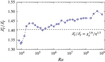
Ratio of the thermal boundary layer thicknesses
 ${\it\lambda}_{T}^{o}/{\it\lambda}_{T}^{i}$
as a function of the Rayleigh number for the numerical models of table 1 with
 ${\it\eta}=0.6$
and
 $g=(r_{o}/r)^{2}$
. The horizontal dashed line corresponds to the predicted ratio
 ${\it\lambda}_{T}^{o}/{\it\lambda}_{T}^{i}$
given in (3.18).

A closer inspection of figure 11(b) and table 1 nevertheless reveals a remaining weak dependence of the ratio
 ${\it\lambda}_{T}^{o}/{\it\lambda}_{T}^{i}$
on the Rayleigh number. This is illustrated in figure 14 which shows
 ${\it\lambda}_{T}^{o}/{\it\lambda}_{T}^{i}$
as a function of
 $\mathit{Ra}$
for the
 ${\it\eta}=0.6$
,
 $g=(r_{o}/r)^{2}$
cases of table 1. Although some complex variations are visible, the first-order trend is a very slow increase of
 ${\it\lambda}_{T}^{o}/{\it\lambda}_{T}^{i}$
with
 $\mathit{Ra}$
(10 % increase over five decades of
 $\mathit{Ra}$
). No evidence of saturation is however visible and further deviations from the predicted ratio (horizontal dashed line) might therefore be expected at larger
 $\mathit{Ra}$
. This variation might cast some doubts on the validity of the previous derivation for higher Rayleigh numbers. This may imply that either the plume separation is not conserved at higher
 $\mathit{Ra}$
; or that the estimate of the average plume spacing is too simplistic to capture the detailed plume physics in turbulent convection.
4. Boundary layer analysis
The Grossmann Lohse (GL) theory relies on the assumption that the viscous and the thermal boundary layers are not yet turbulent. This is motivated by the observation of small boundary layer Reynolds numbers
 $\mathit{Re}_{s}=\mathit{Re}\,{\it\lambda}/d<200$
in experimental convection up to
 $\mathit{Ra}\simeq 10^{14}$
, which remain well below the expected transition to fully turbulent boundary layers (expected at
 $\mathit{Re}_{s}\sim 420$
, see Ahlers et al. (Reference Ahlers, Grossmann and Lohse2009)). The boundary layer flow is therefore likely laminar and follows the Prandtl–Blasius (PB) laminar boundary layer theory (Prandtl Reference Prandtl1905; Blasius Reference Blasius1908; Schlichting & Gersten Reference Schlichting and Gersten2000). The PB theory assumes a balance between the viscous forces, important in the boundary layers, and inertia which dominates in the bulk of the fluid. For the numerical models with unity Prandtl number, this directly implies that the boundary layer thicknesses are inversely proportional to the square-root of
 $\mathit{Re}$
 $$\begin{eqnarray}{\it\lambda}_{U}\sim {\it\lambda}_{T}\sim \mathit{Re}^{-1/2}.\end{eqnarray}$$
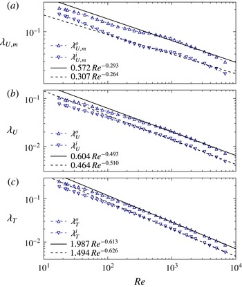
Figure 15(a,b) shows a test of this theoretical scaling for the two different definitions of the viscous boundary layer introduced in § 3.1. Confirming previous findings by Breuer et al. (Reference Breuer, Wessling, Schmalzl and Hansen2004), the commonly employed definition based on the location of the horizontal velocity maxima yields values that significantly differ from the theoretical prediction (4.1). The least-squares fit to the data for the cases with
 $\mathit{Re}>250$
indeed gives values relatively close to
 ${\it\lambda}_{U,m}\sim \mathit{Re}^{-1/4}$
, an exponent already reported in the experiments by Lam et al. (Reference Lam, Shang, Zhou and Xia2002) and in the numerical models in a Cartesian geometry by Breuer et al. (Reference Breuer, Wessling, Schmalzl and Hansen2004) and King et al. (Reference King, Stellmach and Buffett2013). In addition,
 ${\it\lambda}_{U,m}$
is always significantly larger than
 ${\it\lambda}_{T}$
, which is at odds with the expectation
 ${\it\lambda}_{T}\simeq {\it\lambda}_{U}$
when
 $\mathit{Pr}=1$
(see table 1 for detailed values).
(a) Viscous boundary layer thicknesses at the outer boundary (
 ${\it\lambda}_{U,m}^{i}$
) and at the inner boundary (
 ${\it\lambda}_{U,m}^{o}$
) as a function of the Reynolds number for the cases of table 1 (
 ${\it\eta}=0.6$
,
 $g=(r_{o}/r)^{2}$
). (b) Same for the alternative definition of the viscous boundary layer, i.e.
 ${\it\lambda}_{U}^{i}$
and
 ${\it\lambda}_{U}^{o}$
. (c) Thermal boundary layer thicknesses at the outer boundary (
 ${\it\lambda}_{T}^{i}$
) and at the inner boundary (
 ${\it\lambda}_{T}^{o}$
) as a function of
 $\mathit{Re}$
. The black lines in (a–c) correspond to the least-squares fit to the data for the numerical models with
 $\mathit{Ra}\geqslant 10^{6}$
(i.e.
 $\mathit{Re}>250$
).

(a,b) Radial profiles of the time and horizontally averaged temperature
 ${\it\vartheta}$
and horizontal velocity
 $\mathit{Re}_{h}$
. (c)
 ${\it\Theta}$
as a function of
 ${\it\xi}_{T}$
. (d)
 $\mathscr{U}_{h}$
as a function of
 ${\it\xi}_{U}$
. The solid lines in (c,d) corresponds to the Prandtl–Blasius solution. The inset in (c) shows
 ${\it\Theta}$
in double-logarithmic scale. For the sake of clarity, the outer boundary layer is only displayed for one single case in (c,d) (
 $\mathit{Ra}=10^{9}$
,
 ${\it\eta}=0.6$
,
 $g=(r_{o}/r)^{2}$
).

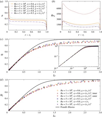
Adopting the intersection of the two tangents to define the viscous boundary layers (figure 15
b) leads to exponents much closer to the predicted value of
 $1/2$
in the high-
 $\mathit{Re}$
regime. The viscous boundary layer thicknesses obtained with this second definition are in addition found to be relatively close to the thermal boundary layer thicknesses in the high Reynolds number regime, i.e.
 ${\it\lambda}_{U}\simeq {\it\lambda}_{T}$
. Therefore, both the expected scaling of
 ${\it\lambda}_{U}$
with
 $\mathit{Re}$
and the similarities between thermal and viscous boundary layer thicknesses strongly suggest that the tangent-intersection method is a more appropriate way to estimate the actual viscous boundary layer. We therefore focus on this definition in the following. For low Reynolds numbers (
 $\mathit{Re}<200$
), however, the viscous boundary layer thicknesses deviate from the PB theory and follow a shallower slope around
 $\mathit{Re}^{-0.4}$
. This deviation implies a possible inaccurate description of the low
 $\mathit{Ra}$
cases by the GL theory (see below).
Figure 15(c) shows that the corresponding scaling of the thermal boundary layer with
 $\mathit{Re}$
follows a similar trend as the viscous boundary layers. The best fit to the data for the cases with
 $\mathit{Re}>250$
yields exponents moderately larger than the theoretical prediction (4.1), while the low-
 $\mathit{Re}$
cases follow a shallower exponent. At this point, we can only speculate that this difference might possibly arise because of the inherent dynamical nature of the thermal boundary layers.
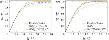
For a meaningful comparison with the boundary layer theory, we define new scaling variables for the distance to the spherical shell boundaries. These variables are introduced to compensate for the changes in the boundary layer thicknesses that arise when
 $\mathit{Ra}$
,
 ${\it\eta}$
or
 $g$
are modified. This then allows us to accurately characterise the shape of both the temperature and the flow profiles in the boundary layers and to compare them with the PB boundary layer profiles. To do so, we introduce the self-similarity variables
 ${\it\xi}_{T}$
and
 ${\it\xi}_{U}$
for both the inner and the outer spherical shell boundaries:
 $$\begin{eqnarray}{\it\xi}_{T}^{i}=\frac{r-r_{i}}{{\it\lambda}_{T}^{i}},\quad {\it\xi}_{T}^{o}=\frac{r_{o}-r}{{\it\lambda}_{T}^{o}},\quad {\it\xi}_{U}^{i}=\frac{r-r_{i}}{{\it\lambda}_{U}^{i}},\quad {\it\xi}_{U}^{o}=\frac{r_{o}-r}{{\it\lambda}_{U}^{o}}.\end{eqnarray}$$
We accordingly define the following rescaled temperatures for both boundaries
 $$\begin{eqnarray}\tilde{T}^{i}(r,{\it\theta},{\it\phi},t)=\frac{T(r,{\it\theta},{\it\phi},t)-{\it\vartheta}(r_{m})}{T_{bot}-{\it\vartheta}(r_{m})},\quad \tilde{T}^{o}(r,{\it\theta},{\it\phi},t)=\frac{{\it\vartheta}(r_{m})-T(r,{\it\theta},{\it\phi},t)}{{\it\vartheta}(r_{m})-T_{top}},\end{eqnarray}$$
where
 $r_{m}=(r_{i}+r_{o})/2$
is the mid-shell radius. The rescaled horizontal velocity is simply obtained by normalisation with its local maximum for each boundary layer:
 $$\begin{eqnarray}\tilde{u} _{h}^{i}(r,{\it\theta},{\it\phi},t)={\displaystyle \frac{u_{h}(r,{\it\theta},{\it\phi},t)}{\max _{i}(\mathit{Re}_{h})}},\quad \tilde{u} _{h}^{o}(r,{\it\theta},{\it\phi},t)={\displaystyle \frac{u_{h}(r,{\it\theta},{\it\phi},t)}{\max _{o}(\mathit{Re}_{h})}}.\end{eqnarray}$$
To check the similarity of the profiles, we consider five numerical models with different
 $\mathit{Ra}$
,
 ${\it\eta}$
and
 $g$
. Figure 16(a,b) show the typical mean horizontal velocity and temperature for these cases, while figure 16(c,d) show the corresponding time and horizontally averaged normalised quantities:
 $$\begin{eqnarray}{\it\Theta}=\overline{\left\langle \tilde{T}_{\phantom{h}}^{i,o}\right\rangle _{s}},\quad \mathscr{U}_{h}=\overline{\left\langle \tilde{u} _{h}^{i,o}\right\rangle _{s}}.\end{eqnarray}$$
As already shown in the previous section, the bulk temperature as well as the boundary layer asymmetry strongly depend on the gravity profile and the radius ratio of the spherical shells. Increasing
 $\mathit{Ra}$
leads to a steepening of the temperature profiles near the boundaries accompanied by a shift of the horizontal velocity maxima towards the walls. Although
 ${\it\vartheta}$
and
 $\mathit{Re}_{h}$
drastically differ in the five cases considered here, introducing the normalised variables
 ${\it\Theta}$
and
 $\mathscr{U}_{h}$
allows to merge all the different configurations into one single radial profile. The upward and downward pointing triangles further indicate that those profiles are also independent of the choice of the boundary layer (at the inner or at the outer boundary). Finally, the solutions remain similar to each other when
 $\mathit{Ra}$
is varied, at least in the interval considered here (i.e.
 $10^{8}\leqslant \mathit{Ra}\leqslant 10^{9}$
). These results are in good agreement with the profiles obtained in the numerical simulations by Shishkina & Thess (Reference Shishkina and Thess2009) that cover a similar range of Rayleigh numbers in cylindrical cells with
 ${\it\Gamma}=1$
.
Figure 16(c,d) also compares the numerical profiles with those derived from the PB boundary layer theory. The time-averaged normalised temperature and velocity profiles slightly deviate from the PB profiles, confirming previous 2-D and 3-D numerical models by Shishkina & Thess (Reference Shishkina and Thess2009), Stevens et al. (Reference Stevens, Verzicco and Lohse2010) and Zhou & Xia (Reference Zhou and Xia2010a
). This deviation can be attributed to the intermittent nature of plumes that permanently detach from the boundary layers (Sun, Cheung & Xia Reference Sun, Cheung and Xia2008; Zhou & Xia Reference Zhou and Xia2010a
; du Puits, Resagk & Thess Reference du Puits, Resagk and Thess2013). When the boundary layer profiles are obtained from a time-averaging procedure at a fixed height with respect to the container frame (i.e.
 ${\it\xi}_{T}$
and
 ${\it\xi}_{U}$
are time-independent), they can actually sample both the bulk and the boundary layer dynamics as the measurement position can be at times either inside or outside the boundary layer (for instance during a plume emission). To better isolate the boundary layer dynamics, Zhou & Xia (Reference Zhou and Xia2010a
) therefore suggested studying the physical properties in a time-dependent frame that accounts for the instantaneous boundary layer fluctuations (see also Zhou et al.
Reference Zhou, Stevens, Sugiyama, Grossmann, Lohse and Xia2010; Stevens et al.
Reference Stevens, Zhou, Grossmann, Verzicco, Xia and Lohse2012; Shishkina et al.
Reference Shishkina, Horn, Wagner and Ching2015).
We apply this dynamical rescaling method to our numerical models by defining local and instantaneous boundary layer thicknesses
 $$\begin{eqnarray}{\it\xi}_{T}^{\ast }({\it\theta},{\it\phi},t)=\frac{r_{o}-r}{{\it\lambda}_{T}^{o}({\it\theta},{\it\phi},t)},\quad {\it\xi}_{U}^{\ast }({\it\theta},{\it\phi},t)=\frac{r_{o}-r}{{\it\lambda}_{U}^{o}({\it\theta},{\it\phi},t)}.\end{eqnarray}$$
As the inner and the outer boundary layers exhibit the same behaviour (figure 16), we restrict the following discussion to the outer boundary layer. Following Zhou et al. (Reference Zhou, Stevens, Sugiyama, Grossmann, Lohse and Xia2010) and Shi, Emran & Schumacher (Reference Shi, Emran and Schumacher2012), the horizontal velocity and temperature profiles are given by
 $$\begin{eqnarray}\displaystyle & \mathscr{U}_{h}^{\ast }({\it\xi}_{U}^{\ast })=\overline{\left\langle \tilde{u} _{h}\left(r,{\it\theta},{\it\phi},t\,|\,r=r_{o}-{\it\xi}_{U}^{\ast }{\it\lambda}_{U}^{o}({\it\theta},{\it\phi},t)\right)\right\rangle _{s}}, & \displaystyle\end{eqnarray}$$
 $$\begin{eqnarray}\displaystyle & {\it\Theta}^{\ast }({\it\xi}_{T}^{\ast })=\overline{\left\langle \tilde{T}\left(r,{\it\theta},{\it\phi},t\,|\,r=r_{o}-{\it\xi}_{T}^{\ast }{\it\lambda}_{T}^{o}({\it\theta},{\it\phi},t)\right)\right\rangle _{s}}. & \displaystyle\end{eqnarray}$$
 $({\it\theta},{\it\phi})$
and for several snapshots. Following Zhou & Xia (Reference Zhou and Xia2010a
) and Stevens et al. (Reference Stevens, Zhou, Grossmann, Verzicco, Xia and Lohse2012), the temperature profiles have been further normalised to a position outside the thermal boundary layer (here
 ${\it\xi}_{T}=5$
or
 ${\it\xi}_{T}^{\ast }=5$
) to ease the comparison with the classical definition of the boundary layer in the fixed reference frame (4.5). Figure 17 shows an example of this dynamical rescaling method applied to a case with
 $\mathit{Ra}=10^{8}$
,
 ${\it\eta}=0.6$
and
 $g=(r_{o}/r)^{2}$
. The temperature and horizontal velocity profiles in the spatially and temporally varying local frame are now in much closer agreement with the PB laminar profiles than those obtained in the fixed reference frame.
(a) Time and horizontally averaged normalised temperature profile in the fixed reference frame (dotted line, (4.5)) and in the dynamical frame (dashed line, (4.7)) for a case with
 $\mathit{Ra}=10^{8}$
,
 ${\it\eta}=0.6$
and
 $g=(r_{o}/r)^{2}$
. (b) Corresponding horizontal velocity profile in the fixed reference frame (dotted line, (4.5)) and in the dynamical frame (dashed line, (4.8)). The solid lines in both panels correspond to the Prandtl–Blasius solution.

Because of the numerical cost of the whole procedure, the dynamical rescaling has only been tested on a limited number of cases. Applying the same method to the numerical model with
 $\mathit{Ra}=10^{9}$
(
 ${\it\eta}=0.6$
,
 $g=(r_{o}/r)^{2}$
) yields nearly indistinguishable profiles from those displayed in figure 17. This further indicates that boundary layers in spherical shells are laminar in the
 $\mathit{Ra}$
range explored here and can be well described by the PB theory, provided the boundary layers are analysed in a time-dependent frame which fluctuates with the local and instantaneous boundary layer thicknesses.
5. Dissipation analysis
5.1. Bulk and boundary layer contributions to viscous and thermal dissipation rates
The prerequisite of a laminar boundary layer appears to be fulfilled in our numerical models and we can thus attempt to apply the GL formalism to our dataset. The idea of the GL theory is to separate the viscous and thermal dissipation rates into two contributions, one coming from the fluid bulk (indicated by the superscript
 $bu$
in the following) and one coming from the boundary layers (
 $bl$
), such that
 $$\begin{eqnarray}{\it\epsilon}_{T}={\it\epsilon}_{T}^{bu}+{\it\epsilon}_{T}^{bl},\quad {\it\epsilon}_{U}={\it\epsilon}_{U}^{bu}+{\it\epsilon}_{U}^{bl},\end{eqnarray}$$
where the contributions from the bulk are defined by
 $$\begin{eqnarray}{\it\epsilon}_{T}^{bu}=\frac{4{\rm\pi}}{V}\int _{r_{i}+{\it\lambda}_{T}^{i}}^{r_{o}-{\it\lambda}_{T}^{o}}\overline{\left\langle ({\rm\nabla}T)^{2}\right\rangle _{s}}\,r^{2}\,\text{d}r,\quad {\it\epsilon}_{U}^{bu}=\frac{4{\rm\pi}}{V}\int _{r_{i}+{\it\lambda}_{U}^{i}}^{r_{o}-{\it\lambda}_{U}^{o}}\overline{\left\langle (\boldsymbol{{\rm\nabla}}\times \boldsymbol{u})^{2}\right\rangle _{s}}\,r^{2}\,\text{d}r,\end{eqnarray}$$
and the boundary layer contributions are given by
 $$\begin{eqnarray}\left.\begin{array}{@{}c@{}}\displaystyle {\it\epsilon}_{T}^{bl}=\frac{4{\rm\pi}}{V}\int _{r_{i}}^{r_{i}+{\it\lambda}_{T}^{i}}\overline{\left\langle ({\rm\nabla}T)^{2}\right\rangle _{s}}\,r^{2}\,\text{d}r+\frac{4{\rm\pi}}{V}\int _{r_{o}-{\it\lambda}_{T}^{o}}^{r_{o}}\overline{\left\langle ({\rm\nabla}T)^{2}\right\rangle _{s}}\,r^{2}\,\text{d}r,\\ \displaystyle {\it\epsilon}_{U}^{bl}=\frac{4{\rm\pi}}{V}\int _{r_{i}}^{r_{i}+{\it\lambda}_{U}^{i}}\overline{\left\langle (\boldsymbol{{\rm\nabla}}\times \boldsymbol{u})^{2}\right\rangle _{s}}\,r^{2}\,\text{d}r+\frac{4{\rm\pi}}{V}\int _{r_{o}-{\it\lambda}_{U}^{o}}^{r_{o}}\overline{\left\langle (\boldsymbol{{\rm\nabla}}\times \boldsymbol{u})^{2}\right\rangle _{s}}\,r^{2}\,\text{d}r.\end{array}\right\}\end{eqnarray}$$
The RB flows are then classified in the
 $\mathit{Ra}{-}\mathit{Pr}$
parameter space according to the dominant contributions to the viscous and thermal dissipation rates. This defines four regimes depending on
 $\mathit{Ra}$
and
 $\mathit{Pr}$
: regime I when
 ${\it\epsilon}_{U}\simeq {\it\epsilon}_{U}^{bl}$
and
 ${\it\epsilon}_{T}\simeq {\it\epsilon}_{T}^{bl}$
; regime II when
 ${\it\epsilon}_{U}\simeq {\it\epsilon}_{U}^{bu}$
and
 ${\it\epsilon}_{T}\simeq {\it\epsilon}_{T}^{bl}$
; regime III when
 ${\it\epsilon}_{U}\simeq {\it\epsilon}_{U}^{bl}$
and
 ${\it\epsilon}_{T}\simeq {\it\epsilon}_{T}^{bu}$
; and finally regime IV when
 ${\it\epsilon}_{U}\simeq {\it\epsilon}_{U}^{bu}$
and
 ${\it\epsilon}_{T}\simeq {\it\epsilon}_{T}^{bu}$
.
For a unity Prandtl number, the GL theory predicts that the flows should be dominated by dissipations in the boundary layer regions at low
 $\mathit{Ra}$
(regime I). A transition to another regime where dissipations in the fluid bulk dominates (regime IV) is expected to happen at approximately
 $\mathit{Ra}\simeq 10^{8}{-}10^{10}$
(Grossmann & Lohse Reference Grossmann and Lohse2000; Ahlers et al.
Reference Ahlers, Grossmann and Lohse2009; Stevens et al.
Reference Stevens, van der Poel, Grossmann and Lohse2013).
Figure 18 shows the relative contributions of the bulk and boundary layers to the viscous and thermal dissipation rates. The viscous dissipation
 ${\it\epsilon}_{U}$
is always dominated by the bulk contribution: starting at approximately 60 % at
 $\mathit{Ra}=10^{4}$
, it nearly reaches 90 % at
 $\mathit{Ra}=10^{9}$
. In contrast, the thermal dissipation rate is always dominated by the boundary layer regions, such that
 ${\it\epsilon}_{T}^{bu}$
slowly increases from 10 % at
 $\mathit{Ra}=10^{4}$
to 30 % at
 $\mathit{Ra}=10^{9}$
. According to the GL classification, all of our numerical simulations thus belong to regime II of the
 $\mathit{Ra}{-}\mathit{Pr}$
parameter space, in which
 ${\it\epsilon}_{U}^{bu}>{\it\epsilon}_{U}^{bl}$
and
 ${\it\epsilon}_{T}^{bl}>{\it\epsilon}_{T}^{bu}$
. This seems at odds with the GL theory, which predicts that our DNS should be located either in regime I or in regime IV of the parameter space for the range of
 $\mathit{Ra}$
explored here (
 $10^{3}\leqslant Ra\leqslant 10^{9}$
).
Measured contributions of the boundary layer (open symbols) and the fluid bulk (filled symbols) to the total viscous dissipation rate
 ${\it\epsilon}_{U}$
(orange squares) and the total thermal dissipation rate
 ${\it\epsilon}_{T}$
(blue circles).

(a) Viscous dissipation in the bulk of the fluid as a function of
 $\mathit{Re}$
. (b) Corresponding compensated
 ${\it\epsilon}_{U}^{bu}$
scaling. (c) Thermal dissipation in the bulk of the fluid as a function of
 $\mathit{Re}$
. (d) Corresponding compensated
 ${\it\epsilon}_{T}^{bu}$
scaling. The solid black lines in the four panels correspond to the least-squares fit to the data for the numerical models with
 $\mathit{Ra}\geqslant 10^{5}$
.

The dominance of the boundary layer contribution in the thermal dissipation rate has already been reported by Verzicco (Reference Verzicco2003) for the same range of
 $\mathit{Ra}$
values. This phenomenon may be attributed to the dynamical nature of the plumes which permanently detach from the boundary layers and penetrate into the bulk of the fluid. These thermal plumes have the same typical size as the boundary layer thickness and can thus be thought as ‘detached boundary layers’. Grossmann & Lohse (Reference Grossmann and Lohse2004) have therefore suggested modifying their scaling theory to incorporate these detached boundary layers in the thermal dissipation rate. They propose to decompose
 ${\it\epsilon}_{T}$
into one contribution coming from the plumes (
 ${\it\epsilon}_{T}^{pl}$
) and one coming from the turbulent background (
 ${\it\epsilon}_{T}^{bg}$
)
 $$\begin{eqnarray}{\it\epsilon}_{T}={\it\epsilon}_{T}^{pl}+{\it\epsilon}_{T}^{bg}.\end{eqnarray}$$
Such a decomposition is however extremely difficult to conduct in spherical shells in which the very large aspect ratio of the convective layer yields a complex and time-dependent multicellular large scale circulation (LSC) pattern (see for instance Bailon-Cuba, Emran & Schumacher Reference Bailon-Cuba, Emran and Schumacher2010, for the influence of large
 ${\it\Gamma}$
on the LSC). In the following, we therefore first retain the initial decomposition (5.1) before coming back to the inherent problem of accurately separating the different contributions to the dissipation rate in § 5.3.
5.2. Individual scaling laws for the dissipation rates
Based on the hypothesis of homogeneous and isotropic turbulence, the GL theory assumes that the thermal and viscous dissipation rates in the bulk of the fluid scale according to
 $$\begin{eqnarray}{\it\epsilon}_{U}^{bu}\sim \mathit{Re}^{3},\quad {\it\epsilon}_{T}^{bu}\sim \mathit{Re},\end{eqnarray}$$
in our dimensionless units. Figure 19 shows the bulk dissipation rates as a function of
 $\mathit{Re}$
for the numerical models of table 1. The best fit to the data (solid lines) for the cases with
 $\mathit{Ra}\geqslant 10^{5}$
yields
 ${\it\epsilon}_{U}^{bu}\sim \mathit{Re}^{2.79}$
and
 ${\it\epsilon}_{T}^{bu}\sim \mathit{Re}^{0.7}$
, are only roughly similar to the prediction (5.5). These deviations from the theoretical exponents are further confirmed by the compensated scalings
 ${\it\epsilon}_{U}^{bu}\,\mathit{Re}^{-3}$
and
 ${\it\epsilon}_{T}^{bu}\,\mathit{Re}^{-1}$
shown in (b) and (d), which show a coherent remaining dependence on
 $\mathit{Re}$
. Even at high Reynolds numbers, there is no evidence of convergence towards the exact expected scalings from the GL theory. This is particularly obvious for
 ${\it\epsilon}_{T}^{bu}$
which remains in close agreement with
 ${\it\epsilon}_{T}^{bu}\sim \mathit{Re}^{0.7}$
for the whole range of
 $\mathit{Re}$
values explored here (solid line in figure 19
d). The dependence of
 ${\it\epsilon}_{U}^{bu}$
on
 $\mathit{Re}$
shows a gradual steepening of the slope when
 $\mathit{Re}$
increases, which implies that
 ${\it\epsilon}_{U}^{bu}(\mathit{Re})$
cannot be accurately represented by a simple power law. Similar deviations from (5.5) have already been reported in the Taylor–Couette flow experiments of Lathrop, Fineberg & Swinney (Reference Lathrop, Fineberg and Swinney1992) and in the numerical simulations of RB homogeneous turbulence of Calzavarini et al. (Reference Calzavarini, Lohse, Toschi and Tripiccione2005).
A similar procedure can be applied to the dissipation rates in the boundary layers. In spherical shells, the volume fraction occupied by the boundary layers can be approximated by the following Taylor expansion to the first-order
 $$\begin{eqnarray}f_{V}({\it\lambda})=\frac{4{\rm\pi}}{V}\left(\int _{r_{i}}^{r_{i}+{\it\lambda}^{i}}r^{2}\,\text{d}r+\int _{r_{o}-{\it\lambda}^{o}}^{r_{o}}r^{2}\,\text{d}r\right)\simeq 3\,\frac{{\it\lambda}^{i}{\it\eta}^{2}+{\it\lambda}^{o}}{1+{\it\eta}+{\it\eta}^{2}},\end{eqnarray}$$
in the limit of thin boundary layers
 ${\it\lambda}\ll r_{o}-r_{i}$
. The viscous dissipation rate in the boundary layers can then be estimated by
 $$\begin{eqnarray}{\it\epsilon}_{U}^{bl}\sim \frac{U_{rms}^{2}}{{\it\lambda}_{U}^{2}}\,f_{V}({\it\lambda}_{U})\sim \frac{\mathit{Re}^{2}}{{\it\lambda}_{U}},\end{eqnarray}$$
in our dimensionless units. As demonstrated in § 4, the boundary layers are laminar and are in reasonable agreement with the PB boundary layer theory. This implies that
 ${\it\lambda}_{U}\sim \mathit{Re}^{-1/2}$
and thus yields
 $$\begin{eqnarray}{\it\epsilon}_{U}^{bl}\sim \mathit{Re}^{5/2}.\end{eqnarray}$$
Figure 20 shows the viscous dissipation rate in the boundary layers as a function of
 $\mathit{Re}$
for the numerical models of table 1. The least-squares fit to the data (solid lines) yields
 ${\it\epsilon}_{U}^{bl}\sim \mathit{Re}^{2.52}$
, in close agreement with the expected theoretical exponent. The compensated scaling displayed in (b) reveals a remaining weak secondary dependence of
 ${\it\epsilon}_{U}^{bl}$
on
 $\mathit{Re}$
, which is not accurately captured by the power law. The local slope of
 ${\it\epsilon}_{U}^{bl}(\mathit{Re})$
initially decreases with
 $\mathit{Re}$
(when
 $\mathit{Re}\lesssim 200$
) before slowly increasing at higher Reynolds numbers (
 $\mathit{Re}\gtrsim 200$
). This behaviour suggests that, although simple power laws are at first glance in very good agreement with the GL theory, they may not account for the detailed variations of
 ${\it\epsilon}_{U}^{bl}(\mathit{Re})$
.
(a) Viscous dissipation in the boundary layers as a function of
 $\mathit{Re}$
. (b) Corresponding compensated
 ${\it\epsilon}_{U}^{bl}$
scaling. The solid black lines in the four panels correspond to the least-squares fit to the data for the numerical models with
 $\mathit{Ra}\geqslant 10^{5}$
.

The boundary layer contribution to the thermal dissipation rate is estimated in a similar way:
 $$\begin{eqnarray}{\it\epsilon}_{T}^{bl}\sim \frac{{\rm\Delta}T^{2}}{{\it\lambda}_{T}^{2}}\,f_{V}({\it\lambda}_{T})\sim \frac{1}{{\it\lambda}_{T}},\end{eqnarray}$$
which yields
 $$\begin{eqnarray}{\it\epsilon}_{T}^{bl}\sim Nu.\end{eqnarray}$$
The laminar nature of the boundary layers also implies
 ${\it\lambda}_{T}\sim \mathit{Re}^{-1/2}$
and thus
 $$\begin{eqnarray}{\it\epsilon}_{T}^{bl}\sim \mathit{Re}^{1/2}.\end{eqnarray}$$
Figure 21 shows
 ${\it\epsilon}_{T}^{bl}$
as a function of
 $\mathit{Nu}$
and
 $\mathit{Re}$
for the cases of table 1. The least-squares fits yield
 ${\it\epsilon}_{T}^{bl}\sim Nu^{0.95}$
and
 ${\it\epsilon}_{T}^{bl}\sim \mathit{Re}^{0.57}$
(solid lines), close to the expected exponents. However, the compensated scalings displayed in (b) and (d) reveal that the linear fit to
 ${\it\epsilon}_{T}^{bl}(\mathit{Nu})$
remains in good agreement with the data, while
 ${\it\epsilon}_{T}^{bl}(\mathit{Re})$
is not accurately described by such a simple fit. The solutions increasingly deviate from the power law at high Reynolds numbers with the local slope of
 ${\it\epsilon}_{T}^{bl}(\mathit{Re})$
gradually steepening with
 $\mathit{Re}$
.
(a) Thermal dissipation in the boundary layers as a function of
 $\mathit{Nu}$
. (b) Corresponding compensated
 ${\it\epsilon}_{T}^{bl}$
scaling. (c) Thermal dissipation in the boundary layers as a function of
 $\mathit{Re}$
. (d) Corresponding compensated
 ${\it\epsilon}_{T}^{bl}$
scaling. The solid black lines in the four panels correspond to the least-squares fit to the data for the numerical models with
 $\mathit{Ra}\geqslant 10^{5}$
.

(a)
 ${\it\epsilon}_{U}$
as a function of
 $\mathit{Re}$
. (b)
 ${\it\epsilon}_{U}$
normalised by the predictions coming from (5.13) (orange triangles) and (5.14) (blue circles) as a function of
 $\mathit{Re}$
. (c)
 ${\it\epsilon}_{T}$
as a function of
 $\mathit{Re}$
. (d)
 ${\it\epsilon}_{T}$
normalised by the predictions coming from (5.13) (orange triangles) and (5.14) (blue circles) as a function of
 $\mathit{Re}$
. The dashed black lines in (c,d) correspond to the equality between the asymptotic scalings and the data.

5.3. Individual versus global scalings
Despite the overall fair agreement with the GL predictions, a close inspection of the dependence of the four dissipation rates on the Reynolds number reveals some remaining dependence on
 $\mathit{Re}$
, which cannot be perfectly described by simple power laws. This is particularly obvious in the boundary layer contributions
 ${\it\epsilon}_{U}^{bl}(\mathit{Re})$
and
 ${\it\epsilon}_{T}^{bl}(\mathit{Re})$
. In addition, both thermal dissipation rates deviate further from the theoretical exponents than their viscous counterparts (see also Verzicco Reference Verzicco2003). One obvious problem is the inherent difficulty in the separation of the bulk and boundary layer contributions already discussed above. The dynamical plumes constantly departing from the boundary layers obviously complicate matters. To check whether the general idea of a boundary layer and a bulk contribution that both scale with the predicted exponents is at least compatible with the total dissipation rates, we directly fit
 $$\begin{eqnarray}\left.\begin{array}{@{}c@{}}\widehat{{\it\epsilon}_{U}}=\widehat{{\it\epsilon}_{U}^{bu}}+\widehat{{\it\epsilon}_{U}^{bl}}=a\,\mathit{Re}^{3}+b\,\mathit{Re}^{5/2},\\ \widehat{{\it\epsilon}_{T}}=\widehat{{\it\epsilon}_{T}^{bu}}+\widehat{{\it\epsilon}_{T}^{bl}}=c\,\mathit{Re}+d\,\mathit{Re}^{1/2}.\end{array}\right\}\end{eqnarray}$$
This leaves only the four prefactors (
 $a,b,c,d$
) as free fitting parameters and yields
 $$\begin{eqnarray}\left.\begin{array}{@{}c@{}}\widehat{{\it\epsilon}_{U}}=\widehat{{\it\epsilon}_{U}^{bu}}+\widehat{{\it\epsilon}_{U}^{bl}}=0.248\,\mathit{Re}^{3}+7.084\,\mathit{Re}^{5/2},\\ \widehat{{\it\epsilon}_{T}}=\widehat{{\it\epsilon}_{T}^{bu}}+\widehat{{\it\epsilon}_{T}^{bl}}=0.004\,\mathit{Re}+0.453\,\mathit{Re}^{1/2}.\end{array}\right\}\end{eqnarray}$$
We then compare this direct least-squares fit of the total dissipation rates to the sum of the individual scalings obtained in the previous section
 $$\begin{eqnarray}\left.\begin{array}{@{}c@{}}\widehat{{\it\epsilon}_{U}}=\widehat{{\it\epsilon}_{U}^{bu}}+\widehat{{\it\epsilon}_{U}^{bl}}=1.756\,\mathit{Re}^{2.79}+2.197\,\mathit{Re}^{2.52},\\ \widehat{{\it\epsilon}_{T}}=\widehat{{\it\epsilon}_{T}^{bu}}+\widehat{{\it\epsilon}_{T}^{bl}}=0.038\,\mathit{Re}^{0.7}+0.268\,\mathit{Re}^{0.57}.\end{array}\right\}\end{eqnarray}$$
The accuracy of the two scalings (5.13) and (5.14) are compared in figure 22, which shows the total viscous and thermal dissipation rates as a function of
 $\mathit{Re}$
for the numerical models of table 1. While the two scalings are nearly indistinguishable on (a,c), the corresponding normalised scalings shown in (b,d) reveal some important differences. The scalings based on the sum of the power laws derived in the last (5.14) are in relatively poor agreement with the data (5 %–10 % error for
 $\mathit{Re}>10^{2}$
) with no obvious asymptotic behaviour. However, the global scalings (5.13) fall much closer to the actual values for the range
 $10^{2}<\mathit{Re}<10^{4}$
, and approach an asymptote for
 $\mathit{Re}>10^{2}$
. The deviations observed for the highest
 $\mathit{Re}$
cases probably have a numerical origin: the averaging timespan used to estimate the dissipation rates are likely too short in the most demanding cases to perfectly average out all the fluctuations.
The total thermal and viscous dissipation rates in our spherical shell simulations are thus better described by the sum of two power laws that follow the GL theory than by the sum of the asymptotic laws derived from the individual contributions, which suffers from an unclear separation of the boundary layer and bulk dynamics.
This result also sheds a new light on the placement of our numerical simulations in the GL regime diagram (figure 18). Equation (5.13) directly provides the estimated relative contributions of the bulk and boundary layers to the viscous and thermal dissipation rates. Figure 23 shows these different contributions for the numerical models of table 1 and reveals a completely different balance than that shown in figure 18. At low Rayleigh numbers, the estimated boundary layer contributions now dominate both the viscous and thermal dissipation rates. The viscous dissipation rate in the fluid bulk gradually increases with
 $\mathit{Ra}$
and dominates beyond
 $\mathit{Ra}>10^{7}$
. The bulk contribution to the thermal dissipation rate exhibits a similar trend, gradually increasing from approximately 5 % at
 $\mathit{Ra}=10^{4}$
to more than 40 % at
 $\mathit{Ra}=10^{9}$
. While the thermal dissipation rate in the fluid bulk never dominates in the regime explored here, our scaling predicts that it will do so for
 $\mathit{Ra}\gtrsim 3\times 10^{9}$
. These values would then locate the numerical models with
 $\mathit{Ra}\leqslant 10^{7}$
in GL regime I of the
 $\mathit{Ra}{-}\mathit{Pr}$
parameter space. The cases with
 $10^{7}<\mathit{Ra}<3\times 10^{9}$
would then belong to regime II. The transition to regime IV, where the bulk contributions dominate the dissipation rates, would then happen around
 $\mathit{Ra}\simeq 3\times 10^{9}$
.
Estimated relative contributions of the boundary layer (open symbols) and the fluid bulk (filled symbols) to
 $\widehat{{\it\epsilon}_{U}}$
(orange squares) and
 $\widehat{{\it\epsilon}_{T}}$
(blue circles) using (5.13).

(a) Nusselt number versus Rayleigh number. (b) Reynolds number versus Rayleigh number. (c) Compensated Nusselt number versus Rayleigh number. (d) Compensated Reynolds number versus Rayleigh number. The power laws given in (a,b) have been derived from a best fit to the cases of table 1 with
 $\mathit{Ra}\geqslant 10^{5}$
. In (c,d), the dashed lines correspond to the numerical solution of (6.1) and the solid lines to the numerical solution of (6.3).

While it is not clear that the contributions inferred from the total dissipation rates actually reflect the exact bulk and boundary layer contributions to
 ${\it\epsilon}_{U}$
and
 ${\it\epsilon}_{T}$
, this separation nevertheless allows us to reconcile the classification of our spherical shell convection models in the
 $\mathit{Ra}{-}\mathit{Pr}$
parameter space with the prediction of the GL theory for a fluid with
 $\mathit{Pr}=1$
. Future work that will better characterise and separate the bulk and boundary layer dynamics might help to reconcile the individual scalings (figure 18) with the global ones (figure 23), especially at low
 $\mathit{Ra}$
. In particular, considering dissipation layers as defined by Petschel et al. (Reference Petschel, Stellmach, Wilczek, Lülff and Hansen2013) instead of classical boundary layers might possibly help to better separate the bulk and boundary layer contributions.
6. Nusselt and Reynolds numbers scalings
Figure 24 shows
 $\mathit{Nu}$
and
 $\mathit{Re}$
as a function of
 $\mathit{Ra}$
for the cases of table 1. A simple best fit to the data for the cases with
 $\mathit{Ra}\geqslant 10^{5}$
yields
 $\mathit{Nu}\sim \mathit{Ra}^{0.289}$
and
 $\mathit{Re}\sim \mathit{Ra}^{0.479}$
, relatively close to
 $\mathit{Nu}\sim \mathit{Ra}^{2/7}$
and
 $\mathit{Re}\sim \mathit{Ra}^{1/2}$
. While reducing the scaling behaviours of
 $\mathit{Nu}$
and
 $\mathit{Re}$
to such simple power laws is a common practice in studies of convection in spherical shells with infinite Prandtl number (e.g. Wolstencroft et al.
Reference Wolstencroft, Davies and Davies2009; Deschamps et al.
Reference Deschamps, Tackley and Nakagawa2010), this description might be too simplistic to account for the complex dependence of
 $\mathit{Nu}$
and
 $\mathit{Re}$
on
 $\mathit{Ra}$
. To illustrate this issue, figure 24(c,d) show the compensated scalings of
 $\mathit{Nu}$
and
 $\mathit{Re}$
. The power laws fail to capture the complex behaviour of
 $\mathit{Nu}(\mathit{Ra})$
and
 $\mathit{Re}(\mathit{Ra})$
and show an increasing deviation from the data at high
 $\mathit{Ra}$
. For instance, the 0.289 scaling exponent obtained for the Nusselt number is too steep for
 $\mathit{Ra}\leqslant 10^{7}$
and too shallow for higher Rayleigh numbers.
The GL theory predicts a gradual change of the slopes of
 $\mathit{Nu}(\mathit{Ra})$
and
 $\mathit{Re}(\mathit{Ra})$
since the flows cross different dynamical regimes when
 $\mathit{Ra}$
increases. Using the asymptotic laws obtained for the different contributions to the dissipation rates (5.14) and the dissipation relations (2.16) and (2.17), we can derive the following equations that relate
 $\mathit{Nu}$
and
 $\mathit{Re}$
to
 $\mathit{Ra}$
:
 $$\begin{eqnarray}\left.\begin{array}{@{}c@{}}\displaystyle {\it\epsilon}_{U}=\frac{3}{1+{\it\eta}+{\it\eta}^{2}}\,\frac{\mathit{Ra}}{\mathit{Pr}^{2}}\,(\mathit{Nu}-1)=1.756\,\mathit{Re}^{2.79}+2.197\,\mathit{Re}^{2.52},\\ \displaystyle {\it\epsilon}_{T}=\frac{3{\it\eta}}{1+{\it\eta}+{\it\eta}^{2}}\,\mathit{Nu}=0.038\,\mathit{Re}^{0.7}+0.268\,\mathit{Re}^{0.57}.\end{array}\right\}\end{eqnarray}$$
This system of equations can be numerically integrated to derive the scaling laws for
 $\mathit{Nu}$
and
 $\mathit{Re}$
. Figure 24(c,d) illustrates the comparison between these integrated values and the actual data, while figure 25 shows the local effective exponents
 ${\it\alpha}_{eff}$
and
 ${\it\beta}_{eff}$
of the
 $\mathit{Nu}(\mathit{Ra})$
and
 $\mathit{Re}(\mathit{Ra})$
laws as a function of
 $\mathit{Ra}$
:
 $$\begin{eqnarray}{\it\alpha}_{eff}=\frac{\partial \ln \mathit{Nu}}{\partial \ln \mathit{Ra}};\quad {\it\beta}_{eff}=\frac{\partial \ln \mathit{Re}}{\partial \ln \mathit{Ra}}.\end{eqnarray}$$
While
 $\mathit{Re}(\mathit{Ra})$
is nicely described by the solution of (6.1), some persistent deviations in the
 $\mathit{Nu}(\mathit{Ra})$
scaling are noticeable. In particular,
 ${\it\alpha}_{eff}(\mathit{Ra})$
increases much faster than expected from the scaling law (dashed lines):
 ${\it\alpha}_{eff}(10^{9})\simeq 0.32$
while the predicted slope remains close to 0.285. The difficulty in accurately separating the bulk and boundary layer dynamics when deriving the scaling laws for the different contributions to the dissipation rates are once again likely responsible of this misfit.


As demonstrated in the previous section, replacing the sum of the individual dissipation contributions by the global scalings provides a much better fit to
 ${\it\epsilon}_{U}$
and
 ${\it\epsilon}_{T}$
(figure 22). We can thus construct another set of equations based on the scaling laws for the total dissipation rates (5.13):
 $$\begin{eqnarray}\left.\begin{array}{@{}c@{}}\displaystyle {\it\epsilon}_{U}=\frac{3}{1+{\it\eta}+{\it\eta}^{2}}\,\frac{\mathit{Ra}}{\mathit{Pr}^{2}}\,(\mathit{Nu}-1)=0.248\,\mathit{Re}^{3}+7.084\,\mathit{Re}^{5/2},\\ \displaystyle {\it\epsilon}_{T}=\frac{3{\it\eta}}{1+{\it\eta}+{\it\eta}^{2}}\,\mathit{Nu}=0.004\,\mathit{Re}+0.453\,\mathit{Re}^{1/2}.\end{array}\right\}\end{eqnarray}$$
This system of equations is once again numerically integrated to derive the scaling laws for
 $\mathit{Nu}(\mathit{Ra})$
and
 $\mathit{Re}(\mathit{Ra})$
. The solid black lines displayed in figures 24(c,d) and 25 show that these scaling laws fall now much closer to the data. They accurately reproduce both
 $\mathit{Nu}(\mathit{Ra})$
and
 $\mathit{Re}(\mathit{Ra})$
for the whole range of Rayleigh numbers, and the gradual change in the slopes
 ${\it\alpha}_{eff}$
and
 ${\it\beta}_{eff}$
are also correctly captured. The improvement of the fit to the data when using (6.3) instead of (6.1) is a direct consequence of the better description of the total dissipation rates by the global scalings (5.13) rather than by the sum of the individual scalings (5.14).
Figures 24(c,d) and 25 also show an extrapolation of the scaling laws, solution of (6.3), up to
 $\mathit{Ra}=10^{11}$
. Interestingly, the scaling laws predict that
 ${\it\alpha}_{eff}$
would become steeper than
 $1/3$
for
 $\mathit{Ra}>5\times 10^{9}$
. This transition point to an enhanced heat transport efficiency would then occur at a much lower
 $\mathit{Ra}$
than in RB convection in Cartesian or cylindrical cells. For instance, the experiments by Roche et al. (Reference Roche, Gauthier, Kaiser and Salort2010) showed an enhanced scaling of
 $\mathit{Nu}\sim \mathit{Ra}^{0.38}$
for
 $\mathit{Ra}>7\times 10^{11}$
. The predicted effective exponent
 ${\it\alpha}_{eff}$
however seems to increase slightly faster than suggested by our numerical data. The possible transition to an enhanced heat transport regime at lower
 $\mathit{Ra}$
than in a planar geometry thus remains an open issue. Furthermore, the extrapolation of the obtained scaling laws to high Rayleigh numbers is debatable since the underlying decomposition (5.13) relies on the assumption of laminar boundary layers, which will not hold beyond the transition point. Future RB models in spherical shells that will possibly reach
 $\mathit{Ra}\simeq 10^{10}$
could certainly help to confirm this trend and check the robustness of the best-fit coefficients obtained in (5.13) (Stevens et al.
Reference Stevens, van der Poel, Grossmann and Lohse2013).
7. Conclusion and outlooks
We have studied Rayleigh–Bénard (RB) convection in spherical shells for Rayleigh numbers up to
 $10^{9}$
and a Prandtl number of unity. Because of both curvature and radial variations of buoyancy, convection in spherical shells exhibits asymmetric boundary layers. To better characterise this asymmetry, we have conducted a systematic parameter study, varying both the radius ratio and the radial distribution of gravity. Two theories were developed in the past to determine this boundary layer asymmetry. The first one by Jarvis (Reference Jarvis1993) and Vangelov & Jarvis (Reference Vangelov and Jarvis1994) hypothesises that both boundary layers adjust their thickness to maintain the same critical boundary layer Rayleigh number; while the second one by Wu & Libchaber (Reference Wu and Libchaber1991) assumes that the thermal fluctuations at mid-depth are statistically symmetrically distributed. Both theories however yield scaling laws in poor agreement with our numerical simulations. On the contrary, we found that the average plume density, or equivalently the average inter-plume spacing, is comparable for both boundary layers. An estimation of the average plume density at both spherical bounding surfaces has allowed us to accurately predict the boundary layer asymmetry and the mean bulk temperature for the wide range of spherical shell configurations explored here (
 ${\it\eta}=r_{i}/r_{o}$
spanning the range
 $0.2\leqslant {\it\eta}\leqslant 0.95$
and gravity profiles of
 $g\in [r/r_{o},\,1,\,(r_{o}/r)^{2},\,(r_{o}/r)^{5}]$
).
Because of the lack of experiments and numerical models of non-rotating convection in spherical shells at finite Prandtl numbers, the scaling properties of the Nusselt and the Reynolds numbers are poorly characterised in this geometry. To further address this question, we have conducted numerical models in spherical shells with
 ${\it\eta}=0.6$
up to
 $\mathit{Ra}=10^{9}$
. We have adopted a gravity profile of the form
 $g=(r_{o}/r)^{2}$
, which has allowed us to conduct a full dissipation analysis. One of the aims of this study was to check the applicability of the scaling theory by Grossmann & Lohse (Reference Grossmann and Lohse2000, Reference Grossmann and Lohse2004) (GL) to convection in spherical shells. One of the prerequisites of this theory is the assumption of Prandtl–Blasius-type (PB) boundary layers. We have thus studied the temperature and horizontal velocity boundary layer profiles. In agreement with the previous findings of Zhou & Xia (Reference Zhou and Xia2010a
), the boundary layer profiles have been found to be in fair agreement with the PB profiles, provided the numerical simulations are analysed in a dynamical frame that incorporates the time and spatial variations of the boundary layers. Following the GL central idea, we have then decomposed the viscous and thermal dissipation rates into contributions coming from the fluid bulk and from the boundary layer regions. The detailed analysis of the individual contributions to the viscous and thermal dissipation rates revealed some noticeable discrepancies to the GL theory (
 ${\it\epsilon}_{U}^{bu}\sim \mathit{Re}^{2.79}$
,
 ${\it\epsilon}_{U}^{bl}\sim \mathit{Re}^{2.52}$
,
 ${\it\epsilon}_{T}^{bu}\sim \mathit{Re}^{0.7}$
and
 ${\it\epsilon}_{T}^{bl}\sim \mathit{Re}^{0.57}$
). The total dissipation rates, however, can nevertheless be nicely described by the sum of bulk and boundary layer contributions that follow the predicted GL exponents (
 ${\it\epsilon}_{U}\sim a\,\mathit{Re}^{3}+b\,\mathit{Re}^{5/2}$
and
 ${\it\epsilon}_{T}\sim a\,\mathit{Re}+b\,\mathit{Re}^{1/2}$
). This strongly suggests that the inaccurate separation of the boundary layer and bulk dynamics is the reason for the inferior fitting of the individual contributions. These scaling laws have finally been employed to study the scaling properties of the Nusselt and Reynolds numbers and provide laws that accurately fit the data. Although these laws exhibit a similar behaviour to experiments and numerical simulations of RB convection in Cartesian or cylindrical coordinates; some distinctions from classical RB cells have also been reported. Our scaling laws predict a continuous increase of the local effective slope of
 $\mathit{Nu}(\mathit{Ra})$
from 0.28 at
 $\mathit{Ra}=10^{6}$
to 0.32 at
 $\mathit{Ra}=10^{9}$
and suggest a possible enhanced heat transfer scaling with an effective exponent steeper than
 $1/3$
for
 $\mathit{Ra}>5\times 10^{9}$
. Similar transitions have been observed in some experiments, though at significantly higher Rayleigh numbers (
 $\mathit{Ra}\sim 10^{11}{-}10^{12}$
, see Roche et al.
Reference Roche, Gauthier, Kaiser and Salort2010).
To explore whether the spherical shell geometry is responsible for this difference, additional numerical simulations at higher Rayleigh numbers are required. Ongoing improvements of pseudo-spectral codes for modelling convection in three-dimensional spherical shells might help to reach spatial resolutions of the order (
 $N_{r}\times \ell _{max}=2048\times 2048$
) in the coming years (e.g. Schaeffer Reference Schaeffer2013). Assuming that the minimum admissible mesh size
 $h$
has to be smaller than the global Kolmogorov scale (Grötzbach Reference Grötzbach1983; Shishkina et al.
Reference Shishkina, Stevens, Grossmann and Lohse2010) yields
 $$\begin{eqnarray}h\leqslant {\it\eta}_{K}=\frac{{\it\nu}^{3/4}}{{\it\epsilon}_{U}^{1/4}}=\left(\frac{1+{\it\eta}+{\it\eta}^{2}}{3}\right)^{1/4}\,\frac{\mathit{Pr}^{1/2}}{\mathit{Ra}^{1/4}\,(\mathit{Nu}-1)^{1/4}}.\end{eqnarray}$$
An extrapolation of the spatial resolutions employed in this study (table 1) then implies that typical resolutions (
 $N_{r}\times \ell _{max}=2048\times 2048$
) might be sufficient to reach
 $\mathit{Ra}\simeq 10^{10}$
for the configuration we considered here (
 ${\it\eta}=0.6$
,
 $g=(r_{o}/r)^{2}$
). This additional decade in
 $\mathit{Ra}$
might already be sufficient to ascertain the derived asymptotic scalings.
Acknowledgements
We thank A. Tilgner for fruitful discussions. All the computations have been carried out on the GWDG computer facilities in Göttingen and on the IBM iDataPlex HPC System Hydra at the MPG Rechenzentrum Garching. T.G. is supported by the Special Priority Program 1488 (PlanetMag, www.planetmag.de) of the German Science Foundation.
Appendix A. Table of results for the numerical models with different geometry and gravity profiles
See table 2.
Summary table of
 $\mathit{Pr}=1$
numerical simulations with various radius ratio
 ${\it\eta}$
and gravity profiles
 $g(r)$
.